Distributed Scheduling in Time Dependent Environments: Algorithms and Analysis
Abstract
Consider the problem of a multiple access channel in a time dependent environment with a large number of users. In such a system, mostly due to practical constraints (e.g., decoding complexity), not all users can be scheduled together, and usually only one user may transmit at any given time. Assuming a distributed, opportunistic scheduling algorithm, we analyse the system’s properties, such as delay, QoS and capacity scaling laws. Specifically, we start with analyzing the performance while assuming the users are not necessarily fully backlogged, focusing on the queueing problem and, especially, on the strong dependence between the queues. We first extend a known queueing model by Ephremides and Zhu, to give new results on the convergence of the probability of collision to its average value (as the number of users grows), and hence for the ensuing system performance metrics, such as throughput and delay. This model, however, is limited in the number of users one can analyze. We thus suggest a new model, which is much simpler yet can accurately describes the system behaviour when the number of users is large.
We then proceed to the analysis of this system under the assumption of time dependent channels. Specifically, we assume each user experiences a different channel state sequence, expressing different channel fluctuations (specifically, the Gilbert-Elliott model). The system performance under this setting is analysed, along with the channel capacity scaling laws.
Index Terms:
QoS, scaling-laws, dependent-channels, EVT, Point-Process.I Introduction
In recent years, connectivity of everyday objects, which are often equipped with computing and networking capabilities, is becoming attractive and in some cases even necessary. These next generation information technologies form the new field of Internet of Things (IoT). A key aspect of such technologies is to support data transfer from a huge number of nodes in the network (e.g., sensors), in order to provide novel applications. For example, many cities today provide smart city technologies such as smart metering, surveillance and security, infrastructure management, city automation, and eHealth. All these applications require data transfer from a huge number of sensors/devices, while sharing a common channel or infrastructure.
Due to this rapid growth in the number of users/devices, which rely on the wireless connectivity to a single gateway, we expect to have extremely large amount of traffic, data or control, and since not all devices can transmit simultaneously, some channel access mechanism is required to coordinate between the transmitters efficiently.
A common channel access for IoT and wireless sensors networks (WSN) is the random access mechanism [1, 2, 3]. Yet, as widely explored over the past few decades, such contention based access paradigms can result in low channel utilization due to collisions and mutual interference. Furthermore, since users are accessing the channel arbitrarily, regardless of their channel quality, a user with bad channel quality can capture the channel and transmit for a long duration (i.e., low rate), degrading the overall network performance [4]. On the other hand, schedule-access-based protocols, allowing a scheduler to schedule users according to their current channel state, hence, exploit the multi-user diversity which is inherent to the wireless medium [5, 6], may suffer from a large overhead and a complexity borden if the number of users is large.
Multi-user diversity gains are even more acute when utilizing multiple antennas both at the transmitter and the receiver. Many scheduling studies can be found for such Multiple-Input Multiple-Output (MIMO) technologies. For examples, in [7] and [8], Zero-Forcing Beamforming (ZFBF) was investigated and user selection was performed in order to avoid interference among users’ streams. Note, however, that such schedule-base schemes involve large channel state information exchange overhead, which hinders the large throughput gain [9].
Considering the above, a suitable channel access scheme can be a distributed opportunistic threshold based algorithm, in which users can attempt transmission only if their channel state is above a threshold. On the one hand, such a scheme is opportunistic as it allows channel access only to users with advantageous channel conditions. On the other hand, it does not require extensive channel state information exchange, hence entails only a relatively low overhead. Several studies in the literature considered similar threshold-based opportunistic systems, e.g., [10, 11] and [12] for the homogeneous and non-homogeneous user cases, respectively. However, these studies investigated only the potential capacity or throughput gains of the mechanism, but have not analyzed other systems’ metrics such as delay or buffer occupancy. Moreover, they did not consider fully the very practical model of a time-dependent channel. [10] have a model with states but it’s a bit different since one state is for no transmission at all and the other allow transmissions.
It is important to note that metrics such as delay or buffer occupancy are especially interesting in threshold-based algorithms, as one might suspect that a threshold-based algorithm will result in a long delay (until the threshold is exceeded) or in some kind of unfair scheduling (if a user exceeds the threshold more often than others).
I-A Main contributions
In this work we address these concerns. Specifically, we consider a multi-user system comprising of users (devices) with a single antenna, wishing to communicate with a single gateway with multiple antennas. The channel access is governed by a threshold based random-access mechanism where each user transmits packets in a first-in-first-out (FIFO) manner, such that packets arriving to a user which is already busy with a pending packet transmission wait for their turn to be transmitted. Accordingly, each user maintains a queue in which it stores packets waiting for transmission. Note that due to the shared medium the queues at different users are tightly correlated. Furthermore, we assume time dependent channels, that is, the channel state users experience is not i.i.d., and depends on the previous channel conditions.
We provide analytical models and closed formulas to determine important properties of such systems. Specifically, the contributions of this work are divided into two main threads which, together, gives a complete understanding of the system. We start with exploring the performance of the system by presenting approximate models for the systems’ queues behavior. We first modify the model presented in [13], while suiting it to our setting. Numerical results and interesting observations are presented for this model. Then, we present a simpler model which, in contrast to the former, is able to describe the system’s behavior when the number of users (hence, queues) is large. In this work-flow, the first model essentially emphasizes the difficulty in tracking such a complex and dependent system, even for time independent channels, while the second model, which is simpler, provides a good answer to this problem by decoupling the dependency between the queues.
We then present a third approximation model, in which we tie the second approximation model with the assumption of time dependent channels. Note that this knot is not possible using the techniques in [13], and is enabled by our simpler decoupling technique. Specifically, we assume that each user experiences a time varying channel modeled as a Good-Bad channel (the Gilbert-Elliot model [14]) which reflects the time varying channel distribution. We thus suggest a time dependent queue model for our multi-user Multiple Access Channel (MAC) system, which shows very good agreement with simulations results.
Finally, after assuming time dependent channels, we study the capacity while considering both the centralized and the threshold-based distributed scheduling algorithms. We achieve closed analytic expressions, in two different ways, for the channel capacity scaling laws. Specifically, we use two statistical tools, Extreme Value Theory (EVT) and Point Process Approximation (PPA). These enable us to examine the limit distribution of the system’s throughput.
The rest of the paper is organized as follows. Section II describes the model and basic assumptions for this work. In Section III, we examine the performance metrics of the queues under this algorithm, e.g., delay and buffer occupancy. Models for the time-independent and time-dependent scenarios are presented along with numerical results. In Section IV, we focus on time-dependent channels and their asymptotic capacity under centralized and distributed algorithms. Section V concludes this work.
II System Model and Assumptions
We consider an uplink system with independent users and one base station. We assume a slotted system in which the time axis is divided into fixed-length intervals, referred to as time slots or simply slots. Following a typical slotted system model, we assume that all nodes are synchronized and that transmissions can only start at slot boundaries. Obviously, simultaneous transmissions may result in collisions. We assume that each user maintains a queue in which the user stores the packets waiting for transmission. The packets are transmitted in a FIFO manner, in which each packet is repeatedly transmitted until received successfully by the base station. We focus our attention on the users’ queues, as illustrated in Figure 1. We assume that the arrival process of new packets to each user’s queue is characterized by a Poisson process. Accordingly, the users are not always backlogged. We further assume that all users are homogenous, thus, all users have the same arrival rate . At the beginning of each slot, each user estimates its own channel conditions, i.e., the expected achievable rate, and tests whether it exceeds a predefined threshold. Upon exceeding and having a packet to send, i.e., if the queue is not empty, the user attempts transmission. Throughout most of this paper the threshold value is set such that on average the probability for exceedance is . Note that it was shown in [10] that under a fully backlogged system this value is optimal. However, considering that users may not have packets to send at all times, the probability of is conservative. That is, it is possible that some slots will not utilized due to over-restrained transmission probability, or alternatively, that the arrival rate, which keeps the system stable, can be slightly higher if we allow users to be slightly more aggressive in their transmission attempts. We emphasise that the analysis presented in this work is correct for any threshold value and arrival rate as long as those maintain stability. We thus give evaluation of different exceedance probabilities via simulations and further discussion regarding the threshold in the sequel.
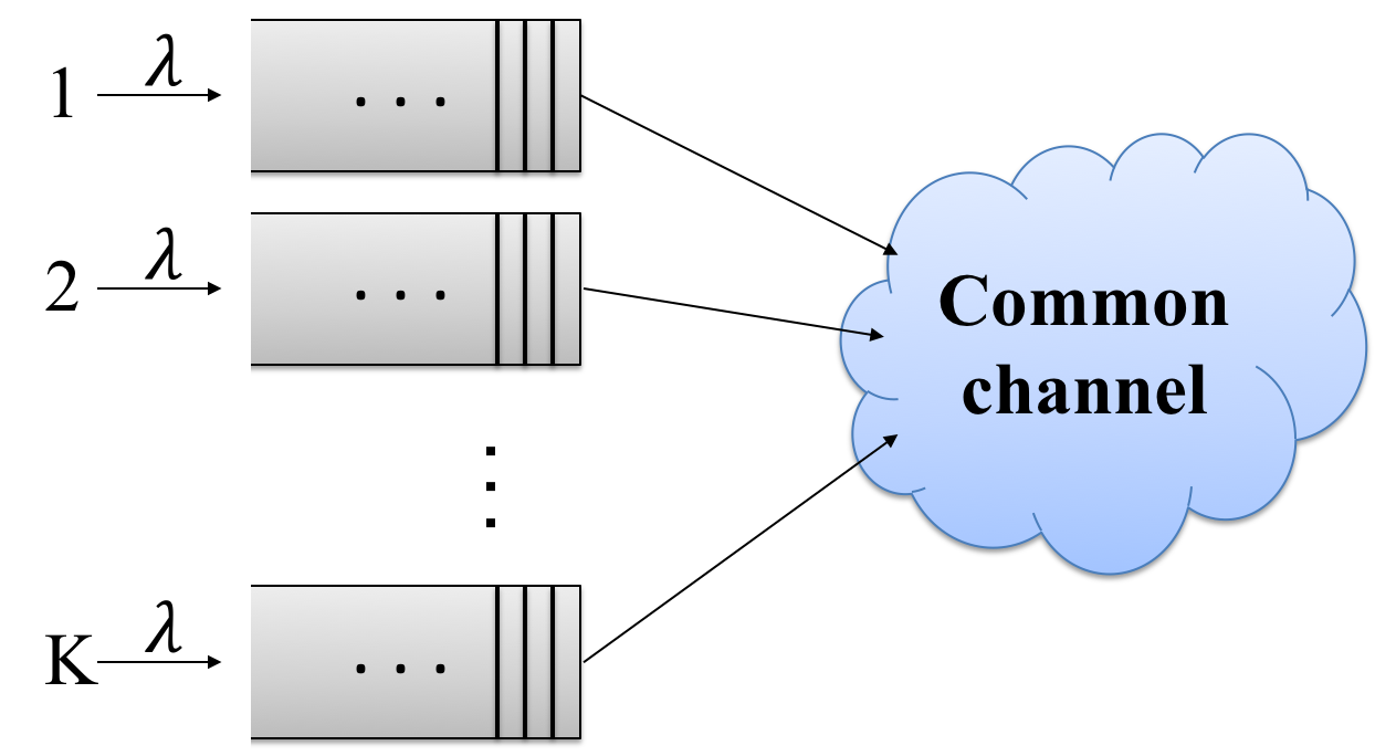
We present several approximate models. Thus, new packets may enter the system at any given (continuous) point on the time axis or at the beginning of a slot, depending on the approximation model used. The slot size is set to encompass a single packet transmission at a rate which corresponds to the threshold. Note that since users are transmitting only while having an above-threshold capacity, and this capacity grows with the number of users [12], the slots are expected to be small, specifically, we may neglect the transmission time in the analysis. In the first part of the paper, we assume that the achievable rates seen by each user at each time slot are i.i.d. We extend these results to a setup in which these achievable rates are still identically distributed yet are not independent. In particular, we assume the channel of each user can alternate between different channel distributions (e.g., Good-Bad channel) according to the Gilbert-Elliot model. A full description will be provided in the sequel.
We define the service time as the time from the moment a packet becomes first in queue, until it is successfully transmitted. Hence, the service time of the packets is composed of the waiting time for transmission and the transmission time.
III Performance analysis
Our system consists of queues, each with an independent Poisson arrival process, and a common server (i.e., the communication channel, Figure 1). A user will attempt transmission only when it is backlogged and the expected transmission rate for the next slot is above a threshold. We assume that any simultaneous transmissions will fail, i.e., no capture. The challenge in analyzing such a queueing system lies in the strong interdependence between the queues. Specifically, the user’s collision or successful transmission probabilities depend on which of the other users’ queues is backlogged (if the threshold exceedance probability is the same for all the users, it depends on the number of backlogged queues). Several works in the literature explored the behavior of various systems with queues interdependency. Due to the interdependence between the queues, each of these works considered a different simplified mathematical model, which resulted in approximations for the required metrics. For example, an iterative approximation model was suggested in [15], utilizing decoupled Markov chains. A refined model was presented in [13]. In [16], the mean delay was given for the case of two identical users, as well as an approximation for a larger population. Extension for slotted CSMA/CD model can be found in [17] and bounds on the stability region for such system can be found in [18].
In the sequel, we investigate the behavior of the system. We start by presenting two different approximations which capture the system performance. The first is a modification of the model presented in [13] to fit a threshold-based system. Different analytical results for the system performance metrics are obtained. The second model uses different technique from the works mentioned above which simplifies the analysis greatly. We extend the analysis for time dependent channels for each user.
III-A Approximation using System and Users’ State
Trying to model the system state as the number of pending packets in each one of the queues, even though straightforward conceptually, is intractable and hence impractical. Accordingly, as our first approximation, we suggest an analytically tractable simplification which relies on the decoupling of the Markov chain into two separate and decoupled chains. This approximation is an adaptation of Ephremides and Zhu’s model presented in [13], which analyzed the slotted ALOHA system with a finite number of buffered nodes. The main difference between the two models is that in slotted aloha described in [13], the transmission scheme is ”immediate first transmission” i.e., if user has an empty queue when a packet arrives, it transmits the packet instantaneously, and in the case of collision, it may transmit again with a retransmission probability , while our model follows a ”delayed first transmission” scheme, where a transmission (first time or a later one) is delayed until the user channel state is favorable, i.e., happens only when the threshold has been exceeded.
As in [13], we assume that the arrival rate at user is , and the arrival processes are statistically independent between the users11 1 This model is able to capture heterogeneous arrival rates. Hence, we keep the subscript in its description. When we turn to the performance analysis we assume that as described in the system model.. Time is slotted and it takes exactly one slot to transmit one packet. We will assume that since the transmission rates are high (users are transmitting only when their expected transmission rate is above a threshold) slot duration is quite small. Furthermore, since we are mainly interested in stable systems, i.e., the inter arrival time is much larger then the slot duration, we will assume that the probability that user receives a new packet for transmission during any given slot is , where is the slot duration. We consider this duration as a unit size. The probability that a user receives more than one packet per slot is, similar to other Poisson models, negligible (i.e., ). Let us denote by the probability that user ’s achievable rate in slot is above the predefined threshold. Since our first model assumes identically distributed channel conditions per slot, we will omit the slot index , i.e., the threshold exceedance probability will be denoted by for all . Accordingly, user attempts to transmit the head-of-the-line packet in its queue (given that its queue is nonempty), with probability . Adopting the model in [13], we define three states in which each user can be at at the beginning of a given slot, namely Idle, Active or Blocked.
The states are determined at the beginning of each slot but depend on the previous slot as well. Specifically, a user is in Idle state in two situations: having an empty queue at the beginning of the current slot, i.e., no packet arrival in the preceding slot, or having one packet in the beginning of the current slot which arrived after the beginning of the preceding slot. A user is in Blocked state if it was backlogged (i.e., its queue was not empty) at the beginning of the previous slot yet it has not transmitted successfully during the previous slot. Note that not transmitting successfully means either there was an unsuccessful transmission attempt, or that there was no transmission attempt at all, i.e., the user’s channel state was below the threshold. A user is in Active state if it is backlogged at the beginning of the current slot and the user has successfully transmitted a packet during the last slot. We emphasize that the Active state is an auxillary state which is utilized in the performance analysis by distinguishing successful transmissions for backlogged users.
Due to the above user ’s transmission probability is:
| (1) |
As previously mentioned, the state space of such a system, which incorporates both the status of each user and the number of pending packets in its queue is intractable. Accordingly, our approximation relies on the decoupling of the Markov chain into two interdependent yet separate chains, the system-status chain and the queue-length chain. The transition probabilities of each chain are tightly depended on the steady-state probabilities of the other chain and thus, all state equations for both chains must be solved simultaneously.
The system-status chain captures the state of each user at any given time. Hence, the status variable consists of ternary variables, , each of which indicates the status of the corresponding terminal. Namely, for Idle, Active and Blocked, respectively. Since the system can incorporate at most one active user at any given time (i.e., at most one user can transmit successfully in the previous slot), it can be shown by summing over all the states where no users are active plus all the possible states in which a single user is active, that the total number of states achievable is . The transition probabilities of the system-status chain, which are different from the one presented in [13], are given in Appendix A. However, we emphasize two quantities which are required for the system-status chain transition probabilities calculation:
| (2) |
Note that these probabilities, which are utilized in the system-status chain solution, reflect the coupling between the two chains. That is, the steady-state probability distribution relies on the queue-length chain steady state. Their calculation can be found in Appendix B.
The queue-length Markov chain tracks both the status and queue length of each user, independently of the status and queue length of the other users. Specifically, the pair represents the state of user , where denotes the total number of packets at queue and is an indicator variable, indicating whether the user is blocked or unblocked (active or idle status), denoted by and , respectively. We further denote by user ’s steady-state probabilities.
The transition probabilities of the chain depend on the following average transmission success probabilities (assuming a user has a packet to send):
| (3) |
where the averaging is performed over the status of the other users (the status of the system). Namely, in order to calculate the probabilities (3), one needs the stationary distribution of the system-status chain . This leads again to the coupling of the two sets of equations. The calculations of these average success probabilities are presented in Appendix B. The conditional moment generating function of the chain for user is defined as
| (4) |
In order to find the steady state probabilities of the decoupled chains, which, as previously explained, must be solved simultaneously, we utilize an iterative process which is based on the Wegstein iteration method. Specifically, at each iteration we exploit the auxiliary quantities computed in the previous iteration to compute , and vice versa. After achieving satisfying convergence, the performance metrics can be calculated using the steady state of the chains.
We emphasize here that due to the ”delayed first transmission” (which is the result of the threshold exceedance requirement) assumption, the transition probabilities of the system chain became quite complicated compared to the analytical derivation in [13].
III-A1 Queueing performance analysis
In this subsection, we analyze the delay a packet endures from the moment it is generated and arrives to a user’s queue until it is successfully transmitted. This delay can be divided into three components: The queueing time to allow the packets already queued to be transmitted, denoted by ; the head-of-the-line waiting time, which is the time elapsed since the packet became first in the queue until successful transmission, denoted by ; the transmission duration which is exactly one slot. Each of them is approximated separately, and the sum of the three gives the total average delay (measured in slot duration):
| (5) |
Our main contributions for the performance analysis are given in the following Theorem, which gives the metrics affected directly from the threshold-based scheduling scheme. That is, the probability for a packet to be blocked is now affected also by the successful exceedance of the threshold and thus the service time is also affected. In addition, the probability for success given a transmission attempt, which was not calculated in [13], is given and will be compared with the approximation model in the next Section.
Theorem 1.
Under the queueing model which follows the ”delayed first transmission” scheme, the performance metrics, i.e., the head-of-the-line waiting time, the probability for a packet to be blocked and the probability for success given a transmission attempt are,
| (6) |
| (7) | ||||
and,
| (8) |
Proof.
The head-of-the-line waiting time takes into account the time the packet spends at the head of the queue excluding the successful transmission slot. Accordingly, the head-of-the-line waiting time is zero both in the case of successful transmission upon arrival at an empty queue (i.e., successful transmission from an Idle state) and in the case of a successful transmission of a backlogged packet, in the slot consecutive to its becoming the head of the queue (i.e., successful transmission from an Active state). Consequently, the head-of-the-line waiting time is the time the packet spends in Blocked state (it is zero for packets which did not pass through Blocked state). Since the number of slots until successful transmission while Blocked is a geometric random variable with mean equal to we have Equation (6).
The probability for a packet to be blocked (Equation (7)) can be computed as the complement of the probability to be unblock (successful transmission without passing through Block state) which is essentially the probability of immediate successful transmission upon arrival of a packet (to the head of the line) which may be only in Idle or Active states. The terms before the success probabilities are the proportion of successful transmissions while in Idle and Active states, respectively.
The probability for success given a transmission attempt (Equation (8)), i.e., the user has packet to send, exceeds the threshold and successfully transmits can be computed as the general success probability regardless the users’ state (Idle, Active, Blocked), divided by the probability for transmission attempt. Note that this event is the result of two independent events, the user channel norm exceeding the threshold and the transmission being successful. Note also that the user can be in Idle state and yet manage to transmit successfully, which can occur upon successful transmission of a packet upon its arrival to an empty queue. ∎
The remaining performance metric, i.e., the queueing time, is calculated, standardly, using Little’s result, hence
| (9) |
where is the average queue length of a user (without considering the blocked head-of-line packet as part of the queue), which is given by [13]:
| (10) |
where .
III-A2 Performance results
In order to gain some insight on the analytical results attained in the previous subsection, in this subsection we present some numerical results. In particular, we present the performance attained by the threshold based channel access mechanism under various metrics such as delay, average queue size and success probability.
The simulation and analytic calculations were performed under homogenous settings in which all users experience the same arrival process and channel distribution. Specifically, the arrival process was approximated by a Bernoulli process in which at each slot each user receives a new packet for transmission with probability . The threshold was set such that the exceedance probability is . Accordingly, each backlogged user examined its channel state at the beginning of each slot, and if its channel state was above a threshold it started transmission. Note that since the channel distribution was homogenous in time, the threshold exceedance process can also be viewed as Bernoulli process in which the transmission probability is . Since, as explained earlier, the number of states in the system-status Markov chain grows exponentially with the number of users, for this model, the simulation and the numerical results were compared only for modest number of users and specifically only for to users. In section III-B we present a model which is able to capture a much larger number of users.
We start by evaluating the effect of the number of users on the average queue length and on the delay, where we divide the delay to its different components, namely, the time in queue and service time. Figures 2(a), 2(b) and 2(c) depict the performance metrics as a function of the number of users, where the total arrival rate is set close to the maximum value which still allows the system to be stable. The results depict very good match between the simulations and the analytic results given in (10), (9) and (6). However, as mentioned earlier, this approximation can only be used for a small number of users.
Figures 2(d), 2(e) and 2(f) depict performance as a function of the total arrival rate, which asserts the following observations: First, for small and moderate values of the arrival rate one can see very good agreement between the analytic results and the simulation. Near the maximum value, however, around the instability region, the values start to diverge, especially in Figures 2(d) and 2(e). These results are consistent with the results of [13], which used small values of as well. The second observation is that as the number of users grows, one can see even stronger compliance with the analytical results. This suggests that this approximate model may be suitable for a large population. Unfortunately, as mentioned before, the calculation of the system steady state is intractable due to the exponential growth of the number of states with the number of users.


Next we compare the estimated success probability given a transmission attempt, with simulation results. Figure 3(a) clearly depicts that the analytical approximation described in (8) matches the simulation results with high accuracy. Even for a small number of seven users we have a difference of only 1.19%. This highly accurate approximation is the foundation for a simplified model, described in the following section, which, in contrast to the model considered thus far, is able to capture the system’s behavior for a large number of users with high accuracy.
III-B Approximation using Constant Collision Probability
As described in the previous section, a user’s success (or conversely, collision) probability depends on the other users’ queues, hence on the system state. That is, different system states will result in different success (collision) probabilities. Trying to solve this set of equations is complicated even for a moderate number of users, all the more so for a large user population. In this section, we present a simpler approach, one which assumes that a user’s collision probability is constant. This will allow us to give close form results which are easy to calculate, and, as simulations depict, are very accurate for large and even moderate for population sizes.
The key approximation method we adopt in this section is inspired by the mean field theory. Mean field theory studies the behavior of a large number of particles which interact. Specifically, when the number of particles is large, mean field approximation suggests an independent evolution of a certain particle relatively to others by approximating the effect of all other particles on that particle by the averaged effect (essentially this is a concentration result). Ever since the mean field approximation was introduced in physics, it was adopted by various fields, including in the context of Markov process models for various dynamic systems. For example, in [19], mean field approximation was used to describe the stability region of the slotted Aloha paradigm. Therein, the authors proved that the distribution of a user’s queue state is not affected by the other users when goes to infinity. Given that, the collision probability can be approximated by a fixed point equation, assuming the probability for empty queue is constant and is independent of the other users. Another seminal work which utilized a constant collision probability as the key approximation is [20], denoted as the decoupling approximation. In this work, a Markov model for the 802.11 back-off process was considered, with users competing on a shared medium. This decoupling assumption can be formally justified as a consequence of convergence to mean field, as the number of users goes to infinity. Several elaborations were made along with verification for the validity of the decoupling approximation [21], [22]. We also note that in [16], independent M/M/1 queues were assumed, with a given distribution on the number of backlogged users. This resulted in an approximation with a varying collision probability. Herein, and similar to the works mentioned above, we assume a constant collision probability which we denote by , i.e., we assume that given a transmission attempt, each user experiences a fixed collision probability regardless of the state or queues of the other users, and regardless of its own state. Even though the mean field theory mostly applies to large and complex stochastic models involving a large number of particles, we will show via simulation that our approach gives high accuracy even for a moderate number of users. We start by investigating the service time.
III-B1 Service time analysis
The service time, which is the time from the moment a packet becomes first in queue, until it is successfully transmitted, depends on the rate at which a user exceeds the threshold and the probability of success (the probability that a collision did not occur). We note that the threshold exceedance process of each user can be modeled as a series of Bernoulli trials. We further note that this process converges to a Poisson process [23], especially if the slot duration is small compared to the time between threshold exceedances. Accordingly, we will approximate the time between threshold exceedances for each user as exponentially distributed with parameter . In the second part of this work, we will prove that indeed, as the number of users grows and the threshold exceedance probability decreases respectfully, convergence exists and exponential distribution between consecutive thresholds exceedances can be considered (see Section IV-B3).
Since we decoupled the queues, we can now assume that each user’s queue behaves like an queue with a feedback loop. Specifically, packets enter each user’s queue according to Poisson process with rate . The inter exceedance interval is exponentially distributed with mean . Upon exceeding the threshold, a packet will be successfully transmitted (hence depart the queue) with probability , and will need to be retransmitted with probability . Accordingly, the queue can be modeled as M/M/1 queue with exponentially distributed service time with parameter . The probability of an empty such queue, is:
| (11) |
where is the number of packets in the queue. We thus have the following lemma:
Lemma 1.
Assume each user’s queue is modeled as an queue with a feedback loop, with an arrival rate , exceedance rate and constant collision probability . Then, the probability for collision satisfies the equation
| (12) |
Hence, for large enough we have the following closed form for
| (13) |
Proof.
Since random selection (with probability ) is performed on the threshold exceedance Poisson process, the outcome successful transmission process is also a Poisson process with rate , which leads to an exponential service time with parameter . Let us examine the probability .
Since the channel quality and the queue length are independent, the probability that a user will attempt transmission, equals the probability that the user is backlogged (i.e., its buffer is not empty) times the probability that its expected rate is above a threshold. Specifically,
| (14) |
On the other hand, given that a user has transmitted, i.e., its expected rate exceeds and its queue is not empty, its collision probability, , is the probability that among all the other users at least one other user will attempt transmission, i.e., at least one other user is backlogged and its expected rate exceeds . This is one minus the probability that no other user has attempted transmission. Thus
which completes the proof. ∎
Equation (13) is an implicit equation and a numerical method is needed in order to find the value of . In Figure 3(a), we depict the numerical calculation of the success probability (the blue line), as given in (13), compared with the approximation derived in the previous section (Eq. (8)) and with simulation results, for different user populations. Although the simple approximation is slightly less accurate for a very small number of users (e.g., around 5% for 4 users) it coincides with the results of the simulation and the approximate model from the previous section (with dependent queues, which cannot be calculated for large ) even for moderate number of users (e.g., around 2% for 10 users). It is important to emphasize that since the number of users is relatively small, we used the equation in its explicit form, meaning without taking to infinity. In Figure 3(b), we compare the average service time computed according to the queue approximation, with service rate , which was calculated according to equation (13), with simulation of the system, which, of course, included dependent queues and variable . Clearly, the approximation shows excellent agreement with the simulation results.

III-B2 Threshold value
The threshold value has a profound effect on the performance. Different threshold values will support different arrival rates, i.e., a different stability region. In addition, the threshold value affects the users’ delay. On the one hand, a high threshold will result in low exceedance probability hence long intervals between transmission attempts. On the other hand, low threshold results in high exceedance probability, hence high collision probability. The optimal threshold value depends on the number of backlogged users in the system at any given time, e.g., when there are only a few backlogged users, a low threshold should be chosen and when many users are backlogged a high threshold should be chosen. Note, however, that the process of monitoring the users at all times, and notifying them regarding the current threshold before each transmission, is not only complex analytically, but mainly impractical in real systems. Therefore, in the analitical part of this work, we focused on a fixed threshold, independent of the users’ status. Specifically, we chose a threshold value such that the probability of exceedance is . This threshold is conservative, as it is designed for the case that all users are backlogged at all times. However, it is interesting to see how a different fixed value affects the results.
Hence, we examine the effect of the threshold on the performance based on simulation results and specifically, we show that a better threshold value can be chosen (which is less conservative). Figures 4(a) and 4(b) depict the throughput and system delay as a function of the exceedance probability, respectively, for 50 users with total arrival rate of . The blue dotted line in Figure 4(a) is the average number of backlogged users as a function of the exceedance probability. Expectedly, when the exceedance probability is high, the throughput decreases and the delay is rapidly growing due to high collision probability. On the other hand, when it is low, throughput decreases as well, due to the long intervals in which no users will attempt transmission, as the threshold is high. This, of course, indicates on the instability of the system. However, as can be seen from figures 4(a) and 4(b), there is a domain of probability values for which the system achieves its maximum throughput and has a low average delay values. One can see that the value of (black dashed line) and the value for which we have a minimum number of backlogged users are found in this domain. It is clear that although the throughput of the system is at its maximum, for this the domain of probability values, the delay and the average number of backlogged users can be reduced if we increase the exceedance probability. A possible criterion for a better excedance probability value may be a threshold which minimizes the average number of backloged users in the system. In addition, we wish to point out that figure 4(b) may be misleading for values which the system is not stable (for and approximately), where one would expect to see an infinite delay. This is due to the run time of the simulation. Nevertheless, we still can see the sharp jump in the delay which indicate its general behaviour.
III-C Approximation using Constant Collision Probability - Time Dependent Channel
In many practical scenarios, the channel seen by a user at a given time slot is correlated with the one seen by the user in the previous time slots. Thus, in the sequel, we will analyze the performance of the threshold based algorithm when users are experiencing a time dependent channel distribution. In particular, we assume that the channel capacity distribution experienced by each user is time varying, according to a Gilbert Elliott model [14]. Specifically, the channel distribution may be at one of two states, denoted as G (for Good) and B (for Bad), where each state determines a different channel distribution. The transitions between the states Good to Bad and Bad to Good follows a Bernoulli distribution with probabilities and , respectively. Thus, the states evolve according to a 2-state Markov chain as described in Figure 5(a). Note that while the trheshold remains fixed, the threshold exceedance probability clearly depends on the user’s channel state. Namely, if a user is in a Good state, the user is expected to exceed the threshold more often than when being in a Bad state. Furthermore, the user’s collision probability not only depends on the number of other backlogged users but also on the channel state of each such backlogged user. Accordingly, trying to solve the system’s stationary distribution, which is one additional dimension over the previous analyzed system, is much more involved than before. We thus adopt the same simplified approach we took in Section III-B. Specifically, we assume that the collision probability that a user experiences is constant regardless of the number of other backlogged users or their channel states. As before, we assume that the slot duration is small compared to the time interval between two consecutive threshold exceedances, even when the user’s channel is in Good state, and approximate the time between threshold exceedances for each user as exponentially distributed with parameter and , depending on whether the user’s channel is in Good or Bad state, respectively. Accordingly, the user’s service time is exponentially distributed with rates or , depending on the user being in Good or Bad state, respectively. Given the Poisson arrival process with rate , the decoupled user’s queue model is presented in Figure 5(b).


This time-dependent queue model can be represented as a continuous Markov process on the set of states for , which indicates the Good or Bad state, and the number of packets in the queue. This two dimensional Markov chain is presented in Figure 5(c). To ease notation, we denote and .
In [24], the authors studied a modification of the queuing model in which the rate of arrival and the service capacity are subject to Poisson alternations. While the model therin is different than the one here, the analysis suggested relied on a Markov chain which is similar to the one presented in Figure 5(c). The system is solved by using generating-function techniques, resulting in a solution for the steady state probabilities, , as a function of the transition rate parameters and the root of a third degree polynomial (only one solution exists under the assumptions). We rely on the solution presented in [24]. Next, we resolve the steady state distribution of the chain.
Let denotes the average service rate.
Note that in order to maintain stability, it is required that . We define the partial generating functions of the system as:
From [24], we have
where is
| (15) | ||||
The steady state probabilities for an empty queue, depending on the channel states, are
| (16) |
where is the root of the polynomial . The remaining steady state probabilities are as follows
| (17) | ||||
From the first derivative of the partial generating functions, we can attain the expected queue size, which includes the head of line packet. Unlike the analysis in subsection III-A, now
Using Little’s theorem, one can attain the average waiting time in the queue,
Note that these aforementioned results rely on and which rely on which is assumed to be fixed, yet is unknown and needs to be computed. Hence, in the same manner as in the previous subsection, we define the probability that a specific user attempts transmission, i.e., exceeds the threshold and its queue is not empty, to be
| (18) | ||||
where the first term consists of the probability to be in a Good state with a packet to transmit, times the probability which an exceedance occurs while existing in the Good state; The second term is similar, referring only to the Bad state. The probability for success, given one user is about to transmit, can be obtained by a similar calculation as in Lemma 1, and we have
| (19) |
Since the root and are coupled, (19) and the roots of the third degree polynomial (15) must be solved simultaneously in order to compute them both.
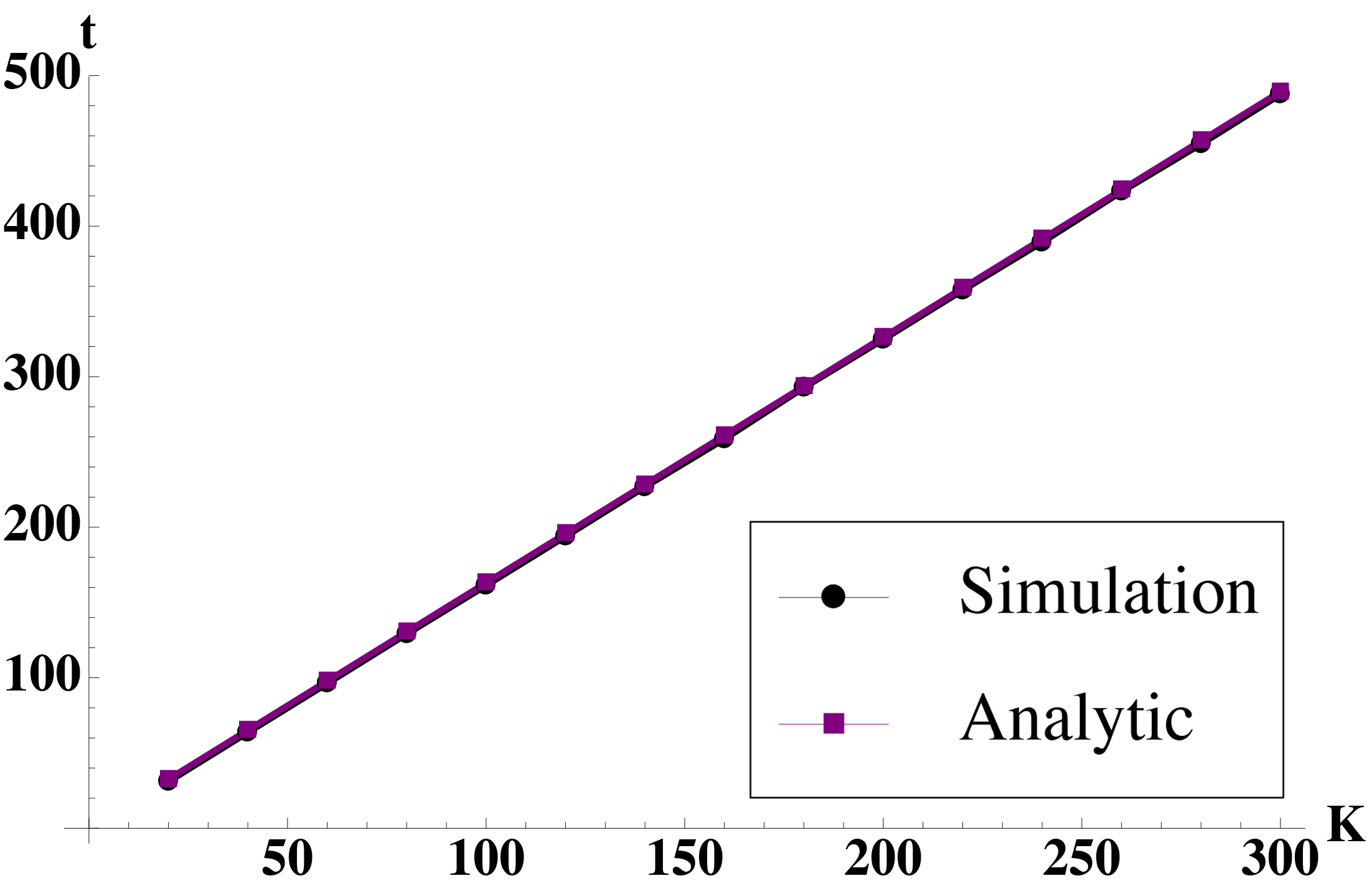
In order to evaluate the approximation, we ran a set of simulation. In the results presented here, the transition rates between Good and Bad states are set equal. Specifically, . The users were considered homogenous. The arrival and service rate parameters, presented in the figures, depict the total rates of the system, and were divided equally among all the users. The service rates were set to and for Good and Bad channel quality, respectively. Figure 6 depicts the probability for success, vs. the number of users for two different arrival rates, and . The figure clearly depicts that the estimated probability for success , coincides with the simulation results for both arrival rates. Figure 7 depicts the mean queue size and the mean sojourn time vs. the number of users for , which also shows good agreement between the approximated analytical results and the simulation results.


IV Scaling Law Under Time Dependent Channel
Up until now, we explored the performance of the MAC system for time independent and time dependent channel scenarios. We considered a distributed threshold based scheduling algorithm, which ensures that when an exceedance occurs, the transmitting user transmits with high channel capacity. This is due to the high threshold value which is set such that only one user will exceed it on average. As mentioned, this scheme exploit multi-user diversity, i.e., let the best user utilize the channel. The scaling laws for independent channels were studied in [10, 11, 12]. However, scaling law of the channel capacity for time dependent channels, to the best of our knowledge, was not considered yet. Hence, in this section, we derive the scaling laws of the channel capacity for our MAC system under the Good-Bad channel model described earlier. We note here that, for this analysis, we consider the users to be backlogged at all time.
We start by formulating the problem and analysing the scaling laws under a centrelized scheduling algorithm, where the base station chooses the strongest user for transmission using the channel state information (CSI) sent to it from the users. We then return to for the distributed algorithm and analyse it as well.
In order to exploit user diversity, the user with the best channel capacity must utilize the channel. Therefore, the problem is in finding the distribution of the random variable , the maximum capacity in a time dependent channel, defined as:
| (20) |
where the capacity of the -th user in each slot is determined by the Good-Bad Markov process :
| (21) |
and are random variables distributed normally with parameters and , respectively. That is, we assume that in each slot, each user exists in either a Good or a Bad state, distinguished by different parameters of the Gaussian distribution which models the capacity. This is due to the Gaussian approximation for the MIMO22
2
The assumption of a MIMO channel is used only to have a concrete expression for the capacity, with a reasonable approximation (in this case, as Gaussian random variable; see e.g., [25]). channel capacity [26, 27]. The parameters reflect the differences in the channel qualities, in a way that a good channel parameters maintain or and .
We are interested in the expected channel capacity at the limit of large . Here, we first use results from EVT, as well as results concerning time dependent processes in order to evaluate the limit distribution of the maximal value when we consider centralized scheduling. Then, when considering distributed scheduling, we use results from PPA in order to analyse threshold arrival rates and tail distributions.
IV-A Centralized Scheduling
Let us consider the distribution of each , as defined in (21), which is determined by the Good-Bad Markov process . The stationary distribution of the chain is , which we will denote in short as . We have
| (22) | ||||
where and are Gaussian distributions with parameters and , respectively. The distribution of the maximal value is in the form of
due to the independence between the users. We wish to test the behaviour of as . Note that this means we actually use the stationary distribution as the marginal distribution.
Our main result in this context is the following.
Theorem 2.
Let be the sequence of the users’ capacities in a certain time slot where each capacity has a distribution as given in (22). Then, the asymptotic distribution of the scheduled user’s capacity, i.e., , is a Gumbel distribution. Specifically,
| (23) |
where
| (24) |
Therefore, the expected throughput of the transmitting user is
| (25) |
where is the Euler-Mascheroni constant.
The proof of Theorem 2 is based on results we obtained on EVT for stationary processes. The complete proof of Theorem 2 is given in Appendix C.
Note that the proof of Theorem 2 is based on the assumption that which implicitly implies that and are bounded away from zero. Nevertheless, note that the expected throughput of the transmitting user when setting , which implies that all users have a Good channel state, agrees with the one presented in [12]. Simulation results for the capacity distribution are given in Figure 8. The figure clearly depicts a match between the analysis and simulation results.
The probability , which is the stationary probability to exist in a Good state, governs the average number of users which are in Good state. That is, in each time slot, one can distinguish between two groups of users: the users that are in a Good state and the users that are in Bad state. It is easy to show that the number of good users, on average, is . Hence, as grows, the expected capacity grows since there are more users in a Good state. This is clear from analytical result in (25) for the channel capacity as well as in Figure 9(c).
One may wonder why considering the bad group at all, meaning, why should a user which is in a Bad channel state be taken into account in the scheduling decision process. Leaving only the users with the good channel to compete for the channel, the capacity with sufficiently large is
| (26) |
Figure 9(c) depicts the influence of the bad group on the capacity. For rather small values of , it is beneficial to schedule the strongest user from both groups. As grows, the size of the good group grows as well, hence the two curves converge to the case were all the users are in Good state. Thus, for small values of the users in the Bad state still have a significant impact, in the sense that they have a high enough probability to be the strongest and gain channel access. Figures 9(a) and 9(b) give a different perspective: the capacity as a function of the number of users. In Figure 9(b), the difference between the capacities is noticeable.


IV-B Distributed Scheduling
One of the main disadvantages in centralized scheduling is the overhead (e.g., CSI) which is needed for communicating properly. Of course for multi-user systems this drawback is more acute. Hence, distributive scheduling schemes become more attractive. One distributive approach which has shown excellent exploitation of multi-user diversity, lets the users transmit based on their instantaneous channel condition [11]. Specifically, given a predefined threshold, users may attempt transmission only if their channel gain exceeds it. When considering this distributed scheduling algorithm, we derive the expected channel capacity using PPA. This method can also be found in [12] for the case of i.i.d. and heterogeneous users. We first give a brief review on the construction of the point process and the relevant results which will be used throughout this subsection.
Let be a sequence of standard normal i.i.d. variables, with the Gumbel Distribution as the extreme value distribution and normalizing constants and . We then define a sequence of points on by:
| (27) |
Under the above, we have the following Theorem.
Theorem 3.
([28]) The sequence on , for some large value of , converge to a non-homogeneous Poisson process with parameter , that is, .
However, since we are interested in time dependent environment, we would like to explore the point process analysis for more general stationary sequences. In [23], exceedances of a high level by a stationary sequence (i.e., points where ), were analyzed, obtaining Poisson limits under weak dependence restrictions. In particularly, the following conditions make precise the notion of extreme events being near-independent if they are sufficiently distant in time.
Definition 1.
We say is strongly mixing if there is a function on the positive integers with as such that, if and for some , then
where denotes the -field generated by the indicated random variables.
When trying to weaken the strong mixing condition, one notes that the events of interest in extreme value theory are typically those of the form . Hence we have,
Definition 2.
([28])
A stationary series is said to satisfy the condition if
for all with ,
where for some sequence such that as .
Another condition which is highly relevant is the local dependence condition :
Definition 3.
([28]) We say that is satisfied if, as ,
Considering the above, we have,
Theorem 4.
([23]) Let hold for the stationary sequence with , such that as for all . Let be the point process, consisting of the exceedances of . Then as , where is a Poisson process with parameter .
Using Theorem 4, we now analyze each user separately and examine its sequence of channel capacities over time. Specifically, we will show that the exceeding points in this dependent sequence converge to a Poisson process, similar to a one if the sequence was i.i.d..
The sequence depends on which state user exists in, which is, in turn, governed by the underlying Markov chain process , as defined in (21). Such processes have been studied before, [29, 30], and are known as processes or ”chain-dependent” processes. In our context, we shall consider the sequence as the sequence of capacities of the i-th’ user over time, and the chain process as the sequence of the irreducible, aperiodic, 2-state Good-Bad Markov chain . Since we analyze the capacity process of one user, and all have the same distribution we omit the user index. We have
| (28) | ||||
where is the transition matrix of the chain and , where belongs to the state space, are the distribution functions associated with the chain states, respectively. Note that each state determines the distribution of for the current time transition. This means that given the chain process , the random variables of the process are conditionally independent. If the initial distribution of the chain is the stationary distribution, i.e for all in the finite state space, where is the stationary distribution, then the distribution of is . In [30], it was stated that every stationary chain-dependent process is strongly mixing. We will show that the process, as defined in this paper, is indeed strongly mixing by definition 1.
Lemma 2.
is strongly mixing with , where is the stationary distribution of the chain and .
Proof.
Let and be as definition 1. Then
For each , as . This was also used in [31] in order to show the strongly mixing property, nevertheless, it is easy to notice that ,in fact, as , regardless of . ∎
Since strong mixing holds for our sequence of channel capacities, due to the fact that it is a weaken case, so does the condition hold. We would like to show that condition also holds, so we are able to characterize the rate of exceedance over the threshold . Note that we are only interested in a sequence of reals which satisfies when considering the condition. We thus have the following Lemma.
Lemma 3.
The local dependence condition holds for the sequence as defined in (21).
Proof.
In the above chain, (a) is since once is known, and are independent, then we conditioned on . (b) is true since maintains , so we have
and therefore
Note that and are constants. ∎
Thus, in our paradigm, a single users’ channel capacity process has the same laws of convergence as if the sequence was i.i.d. with a marginal distribution . Therefore, since the users are independent and each user sees the same marginal distribution , we can analyze the point process of the sequence of all users’ capacities at a specific time (e.g, time slot), resulting in the basic case of i.i.d. random variables, as given in Theorem 3. Considering the above, we can now turn to evaluate the expected channel capacity.
IV-B1 Distributed Algorithm
Given the number of users, we set a capacity threshold such that only a small fraction of the users will exceed it. At the beginning of each slot, each user estimates its capacity for that slot. If the capacity anticipated by the user is greater than the capacity threshold, it transmits in that slot. Otherwise, it keeps silent. The threshold value is set such that one user exceeds the threshold on average, and as a result, its transmission is successful. We treat this slot as a utilized slot. Hence the expected channel capacity has the form:
For the calculation of , the expected capacity experienced by a user who passed , one needs to evaluate the distance of the exceeding points from the threshold. [12] gives the analytical tools to compute the tail distribution of the exceeding points. These points follow the generalized Pareto distribution, hence by using the PPA exceedance rate results, and since we already showed that we have the same exceedance as an i.i.d. case with as the marginal distribution, the result is the same and we have
where is the normalizing constant as in Theorem 2.
We say that a slot is utilized if only one point out of all points exceeds the threshold. Hence, as
where the threshold was chosen such that . We will elaborate on this value in the next subsection. The expected channel capacity is thus
| (29) |
Clearly, in order to assess the expression above and understand how the capacity scales in a distributed algorithm, one has to compute the value of the threshold.
IV-B2 Threshold Estimation
The threshold is set such that only one user on average exceeds it in each time slot. This selection maximizes the probability of a successful transmission in a slot, and is asymptotically optimal as [10]. By using this rule we can estimate the optimal threshold value for the time dependent channel as well:
where the above represents the probability that a user capacity will exceed the threshold . With similar derivation as in Theorem 2 we get that
| (30) |
Putting (30) in (29) we get the same expression for the expected channel capacity under distributed scheduling which show that both approaches have the same scaling laws, the distributed approach being smaller only by a factor of , so there was no loss of optimality due to the distributed algorithm.
IV-B3 Threshold exceedance process
We saw that the point process described earlier result in convergence of the points exceeding to a non-homogeneous Poisson process . This justify our initial assumption, in the performance part of this work, that the time between threshold exceedances is exponentially distributed with parameter . It is important to note that convergence in distribution happens if we change the ”time scale” by a factor of as defined in the definition of in (27). Meaning, we have a point process in the interval and the exceedance of such points has a limiting Poisson distribution. Of course when considering random arrivals it would interest us to assess the convergence of the exceeding points for the entire positive line and not just the unit interval.
Here, we shall use the notation given in [28] for the Poisson properties of exceedance.
Let , a sequence of i.i.d. r.v.s with distribution , be the channel capacity draws of a specific user. From [28, Theorem 2.1.1], if satisfies , then for
where is the number of exceedances of a level by .
By [28, Theorem ], if for each , there exists a sequence satisfying as , and that hold for all , then for any fixed , converges in distribution to a Poisson process on with parameter .
Clearly, for the approximation model given in Section III-B, the dependence conditions hold, since the sequence is i.i.d., so one only needs to show that the first condition holds for each . As for the approximation model given in Section III-C, we already showed that the dependence conditions holds and similar derivation will show that the first condition holds also for each .
Lemma 4.
Assume F is the Gaussian distribution and let and be given according to [28, Theorem 1.5.3]. Fix any and set Then,
Proof.
In a similar way for the derivation of the normalizing constant in [28, Theorem 1.5.3]. Let us find which satisfies the equivalence condition for the convergence of the expression
where the second line is true due to the Gaussian relation as , which in our case grows with . So
we know that , hence
where the penultimate line is due to Taylor expansion. ∎
Now, since all conditions for convergence hold, and the exceeding points indeed converge to a Poisson process on the real line of the exceeding points, we can conclude that a user attempts transmission at a rate of , assuming he has packets to send. Figure 10 show simulation for convergence on the real line.
V Conclusion
In this work, we investigated the performance and the channel capacity of a multi-user MAC system in a time dependent and independent environment under distributed scheduling. Specifically, the performance of the system was derived while considering queueing theory aspects. In fact, a precise characterization is a very difficult mission, which up until today was not solved. Therefore, we presented approximation models to describe its behaviour. First, we addressed the i.i.d. case, where the users do not experience a time varying channel. For that case, we elaborated an existing model and showed results for our paradigm. In addition, we gave another approach, which assumed the queues are independent, derived the probability of collision in the random access mechanism, and enabled us to consider them each as a much more simple queue. Then, we suggested a queue model, which is time dependent and modelled by our Good-Bad channel model. We showed good agreement between the analytic models and the simulation results. Lastly, the expected channel capacity gain was derived in the case where the dependent capacity sequence was modelled as a stationary process, characterized by the Good-Bad channel Markov process.
Appendix A System-status chain transition probabilities
Here we show the calculation of the transition probabilities of the system chain. We use the guide lines in [13] to simplify things and use also their notions but under our case which state that . Due to this fact there are many more possible transition is the state space and therefore the following calculations would be more complicated. In the same manner the calculations are based on the change in the number of active users, thus the transitions can be classified into four types as follows:
- 1.
The number of active users transits from 0 to 1:
Only a blocked user may become active, and only one, say . All other blocked blocked must not exceed the threshold. In addition all idle users which may receive a package must not exceed the threshold and therefore, say , becomes blocked. The latter will repeat it self during this calculation. The probability of such a transition is expressed by:where the product is on the sets of users by their transition and is the number of blocked users after the transition. Note that the user will be active if his queue is not empty after the successful transmission or a package arrived in the beginning of the slot. Also note that and stand for and , respectively.
- 2.
The number of active users remains 1:
This case divides to two subcases, the same active user remains active or another blocked user becomes active. Nevertheless idle users may still become blocked.- (a)
the probability for the first case is:
- (b)
the probability for the second case is:
- (a)
- 3.
The number of active users transits from 1 to 0:
This case is subdivided to three subcases,- (a)
The first subcase is that the active user becomes idle:
- (b)
The second subcase is that the active user becomes blocked and blocked user becomes idle:
- (c)
The third subcase is that the active user becomes blocked:
The first expression is for the case which non of the users exceeds the threshold. The second is for the case which one idle user managed to successfully transmits. The third case describes the case which one or more from the blocked and the idle groups tries to transmit, therefore what happens with user is meaningless. The forth expression describes the situation which user collided with one or more users from the blocked group, or collision happened between the blocked users and didn’t exceed the threshold. The fifth expression is the same as the fourth concerning the group of idle users which receives a package.
- (a)
- 4.
The number of active users remains 0 :
This case is subdivided to three subcases,- (a)
The first subcase is that all users maintain their status without change:
where the first term is the probability that no packet arrives at the idle users while no blocked user, or at least two blocked users, transmit, and the second term is the probability that no blocked user exceeds the threshold while only one of the idle users successfully transmits.
- (b)
The second subcase is that one blocked user becomes idle:
- (c)
The third subcase describes some situation for idle users becomes blocked:
The first expression is for the case which non of the users exceeds the threshold and no blocked user, or at least two blocked users, transmit, the second is for the case which at least two users from exceeds the threshold, the third case describes collision between one of the users from with at least one from the blocked users and the forth expression describes the situation which one idle user succussed to transmit while all the other does’t exceed the threshold.
- (a)
According to these transition probabilities we can calculate the steady state of the chain given the auxiliary quantities and , the probability of exceedance and the users arrival rates.
Appendix B Average success probabilities
Once the steady state of the system chain is known, the average success probabilities can be calculated. We do so by calculate the values of and in the same manner as calculated in [13] while taking in consideration that user must exceed the threshold in order to transmit.
- 1.
For Blocked user :
where
The exponent equals when it’s condition holds.
- 2.
For Active user :
where
the difference here is due to the fact that no more than one user may be active.
- 3.
For Idle user :
where
and
After knowing the these values the boundary conditions can be calculated:
where,
| (31) |
| (32) |
| (33) |
| (34) |
| (35) |
Appendix C Convergence to Extreme Value Distribution
Proof.
Using the stationary distribution as the marginal distribution does not impairs the convergence when , as shown in [30], for such type of dependent sequences. Thus, we can analyze the expected channel capacity using EVT with the distribution above as the marginal distribution function for each user. In order to do so, one first need to prove that convergence to one of the extreme distributions types exists, and derive normilizing constants and . The result in [28, 1.6.2] gives a necessary and sufficient condition on the marginal distribution to belong to each of the three possible domains of attraction of the extreme value distributions.
The first sufficient condition states that if has a negative derivative for all in some interval for , and
| (36) |
then is in the domain of attraction of Type I extreme value distribution (Gumbel distribution). The second necessary and sufficient condition for to be in the domain of attraction of Type I extreme value distribution, states that there exists some strictly positive function such that
| (37) |
for all real .
In the following we give compliance for the convergence conditions and the derivation of and . The stationary distribution as shown earlier has a negative derivative from till . So we only need to show that (36) holds,
In [32], 7.1.13, we can find upper and lower bounds for the complementary error function,
where these inequalities are true for which fits our case for . Using these bounds we will show with the sandwich rule that the limit above converge to . Let us consider first the lower bound of the complementary error function,
The Limit above can be break to four different limits,
please notice that the first and the second limits are similar with the exception of their indexes, and so does the third and the fourth limit. We start with the first limit calculation,
So,
Note that in (a) we assume that . This assumption implies that the situation which all the users are in the bad group is not taken in consideration. For that case all the users have the same channel and the analysis is known and not in our interest. In the same manner we assume also that for the opposite situation. Hence, the first limit result is
As mentioned earlier the first and the second limits different only in their indexes, therefore the result for the second limit is
We turn now for the third limit calculation
The fourth limit also share the same result, and if we add all the parts we can see that the limit converge to . If we consider the upper bound of the complementary error function we will find also that the limit convergence to since the analytical development is the same and the limit
Therefore we can conclude that condition (36) holds for our stationary distribution. We now show that the second condition (37) also holds for the stationary distribution. Let us examine the expression:
Since is a Gaussian distribution we shall use the asymptotic relation:
| (38) |
where (a) is true since
assuming . So taking in consideration condition (37):
By choosing as the strictly positive function for we get
That conclude that the distribution function belongs to the domain of attraction of Type I. Similar analysis can be found in [33], where some examples for convergence of sequences of independent random variables with the same mixed distribution is investigated.
We now derive the normalizing constants and :
According to EVT results for i.i.d. sequences [28, Theorem 1.5.1], is a sequence of real numbers such that as , therefore in our case:
where . The same way as the previous proof using (38) we obtain that
the last step is true since as , similar to the pervious proof.
| (39) |
It follows at once that , and hence
Putting this in (39) ,we obtain
or
and hence
so by using expansion we have,
since we know that we conclude that
∎
References
- [1] N. K. Pratas, H. Thomsen, Č. Stefanović, P. Popovski, Code-expanded random access for machine-type communications, in: Globecom Workshops (GC Wkshps), 2012 IEEE, IEEE, 2012, pp. 1681–1686.
- [2] K. Zhou, N. Nikaein, R. Knopp, C. Bonnet, Contention based access for machine-type communications over LTE, in: Vehicular Technology Conference (VTC Spring), 2012 IEEE 75th, IEEE, 2012, pp. 1–5.
- [3] P. Huang, L. Xiao, S. Soltani, M. W. Mutka, N. Xi, The evolution of MAC protocols in wireless sensor networks: A survey, IEEE communications surveys & tutorials 15 (1) (2013) 101–120.
- [4] M. Heusse, F. Rousseau, G. Berger-Sabbatel, A. Duda, Performance anomaly of 802.11 b, in: INFOCOM 2003. Twenty-Second Annual Joint Conference of the IEEE Computer and Communications. IEEE Societies, Vol. 2, IEEE, 2003, pp. 836–843.
- [5] P. Viswanath, D. N. C. Tse, R. Laroia, Opportunistic beamforming using dumb antennas, Information Theory, IEEE Transactions on 48 (6) (2002) 1277–1294.
- [6] X. Liu, E. K. Chong, N. B. Shroff, Opportunistic transmission scheduling with resource-sharing constraints in wireless networks, Selected Areas in Communications, IEEE Journal on 19 (10) (2001) 2053–2064.
- [7] J. Kim, S. Park, J. H. Lee, J. Lee, H. Jung, A scheduling algorithm combined with zero-forcing beamforming for a multiuser MIMO wireless system, in: IEEE Vehicular Technology Conference, Vol. 1, 2005, pp. 211–215.
- [8] T. Yoo, A. Goldsmith, On the optimality of multiantenna broadcast scheduling using zero-forcing beamforming, Selected Areas in Communications, IEEE Journal on 24 (3) (2006) 528–541.
- [9] O. Bejarano, E. Magistretti, O. Gurewitz, E. W. Knightly, MUTE: sounding inhibition for MU-MIMO WLANs, in: Sensing, Communication, and Networking (SECON), 2014 Eleventh Annual IEEE International Conference on, IEEE, 2014, pp. 135–143.
- [10] X. Qin, R. Berry, Exploiting multiuser diversity for medium access control in wireless networks, in: INFOCOM 2003. Twenty-Second Annual Joint Conference of the IEEE Computer and Communications. IEEE Societies, Vol. 2, IEEE, 2003, pp. 1084–1094.
- [11] X. Qin, R. A. Berry, Distributed approaches for exploiting multiuser diversity in wireless networks, Information Theory, IEEE Transactions on 52 (2) (2006) 392–413.
- [12] J. Kampeas, A. Cohen, O. Gurewitz, Capacity of distributed opportunistic scheduling in nonhomogeneous networks, IEEE Transactions on Information Theory 60 (11) (2014) 7231–7247.
- [13] A. Ephremides, R.-Z. Zhu, Delay analysis of interacting queues with an approximate model, Communications, IEEE Transactions on 35 (2) (1987) 194–201.
- [14] E. N. Gilbert, et al., Capacity of a burst-noise channel, Bell Syst. Tech. J 39 (9) (1960) 1253–1265.
- [15] T. N. Saadawi, A. Ephremides, Analysis, stability, and optimization of slotted ALOHA with a finite number of buffered users, Automatic Control, IEEE Transactions on 26 (3) (1981) 680–689.
- [16] M. Sidi, A. Segall, Two interfering queues in packet-radio networks, Communications, IEEE Transactions on 31 (1) (1983) 123–129.
- [17] H. Takagi, L. Kleinrock, Mean packet queueing delay in a buffered two-user CSMA/CD system, IEEE transactions on communications 33 (1985) 1136–1139.
- [18] W. Luo, A. Ephremides, Stability of n interacting queues in random-access systems, Information Theory, IEEE Transactions on 45 (5) (1999) 1579–1587.
- [19] C. Bordenave, D. McDonald, A. Proutiere, Asymptotic stability region of slotted aloha, Information Theory, IEEE Transactions on 58 (9) (2012) 5841–5855.
- [20] G. Bianchi, Performance analysis of the IEEE 802.11 distributed coordination function, Selected Areas in Communications, IEEE Journal on 18 (3) (2000) 535–547.
- [21] D. Malone, K. Duffy, D. Leith, Modeling the 802.11 distributed coordination function in nonsaturated heterogeneous conditions, Networking, IEEE/ACM Transactions on 15 (1) (2007) 159–172.
- [22] J.-w. Cho, J.-Y. Le Boudec, Y. Jiang, On the asymptotic validity of the decoupling assumption for analyzing 802.11 MAC protocol, Information Theory, IEEE Transactions on 58 (11) (2012) 6879–6893.
- [23] M. Leadbetter, Weak convergence of high level exceedances by a stationary sequence, Probability Theory and Related Fields 34 (1) (1976) 11–15.
- [24] U. Yechiali, P. Naor, Queuing problems with heterogeneous arrivals and service, Operations Research 19 (3) (1971) 722–734.
- [25] O. Shmuel, A. Cohen, O. Gurewitz, Capacity of wireless systems under distributed scheduling of time-dependent users, in: Electrical & Electronics Engineers in Israel (IEEEI), 2014 IEEE 28th Convention of, IEEE, 2014, pp. 1–5.
- [26] P. J. Smith, M. Shafi, On a gaussian approximation to the capacity of wireless MIMO systems, in: Communications, 2002. ICC 2002. IEEE International Conference on, Vol. 1, IEEE, 2002, pp. 406–410.
- [27] M. Chiani, M. Z. Win, A. Zanella, On the capacity of spatially correlated MIMO rayleigh-fading channels, Information Theory, IEEE Transactions on 49 (10) (2003) 2363–2371.
- [28] M. R. Leadbetter, Extreme and related properties of random sequences and processes, Springer-verlag, 1983.
- [29] J. Janssen, Les processus (jx), Cahiers du CERO 11 (1969) (1969) 181–214.
- [30] G. Denzel, G. O’Brien, Limit theorems for extreme values of chain-dependent processes, The Annals of Probability (1975) 773–779.
- [31] G. O’Brien, Limit theorems for sums of chain-dependent processes, Journal of applied probability (1974) 582–587.
- [32] M. Abramowitz, I. A. Stegun, Handbook of mathematical functions: with formulas, graphs, and mathematical tables, Courier Dover Publications, 2012.
- [33] P. Mladenović, Extreme values of the sequences of independent random variables with mixed distributions, Matematički Vesnik (212) (1999) 29–37.