Inflationary attractors from nonminimal coupling

The Planck measurements of the cosmic microwave background anisotropies give the scalar spectral tilt $n_{s}=0.968\pm 0.006$ and the tensor to scalar ratio $r_{0.002}<0.11(95\%\text{C.L.})$[1, 2]. The central value of $n_{s}$ suggests the relation $n_{s}=1-2/N$ with $N=60$, here $N$ is the number of $e$-folds when the pivotal scale exits the horizon before the end of inflation. To the leading order of $1/N$, many inflation models have the universal result $n_{s}=1-2/N$, they include the $R^{2}$ inflation[3] and the hilltop inflation[4], the Higgs inflation with the nonminimal coupling $\xi\phi^{2}R$[5, 6] also gives the same $n_{s}$ when $\xi\gg 1$, which is a special case of the more general nonminimal coupling $\xi f(\phi)R$ with the potential $\lambda^{2}f^{2}(\phi)$ for an arbitrary function $f(\phi)$ in the strong coupling limit $\xi\gg 1$[7]. The above relation between $n_{s}$ and $N$ can be generalized to the parametrization of the observables in terms of $N$ and used to reconstruct inflationary potential [8, 9, 10, 11, 12, 13, 14, 15, 16, 17, 18, 19].

In this talk, we show that in the strong coupling limit $\xi\gg 1$, any attractor is possible for the nonminimal coupling $\xi f(\phi)R$ with an arbitrary coupling function $f(\phi)$ [20]. The E-model attractor is used as an example to support the claim. The talk is organized as follows. In section 2, we discuss the Higgs inflation. The construction of attractor behaviours is discussed in section 3. The conclusions are drawn in section 4.

The simplest and easiest way to realize the cosmic inflation is to use scalar fields. Until now, the only scalar field observed is Higgs field. The Higgs potential is

$$V(\phi)=\frac{\lambda}{4}\left(\phi^{2}-v^{2}\right)^{2},$$

(1)

where we set $c=\hbar=1/8\pi G=1$. Because $v\sim 100\text{GeV}$ and $\phi\sim 10^{19}\text{GeV}$, we can neglect the parameter $v$ and consider the simple power-law potential [21]

$$V_{h}(\phi)=\frac{\lambda}{4}\phi^{4}.$$

(2)

The action for the Higgs field minimally coupled to gravity is

$$S=\int d^{4}x\sqrt{-g}\left[\frac{1}{2}R-\frac{1}{2}g^{\mu\nu}\nabla_{\mu}\phi\nabla_{\nu}\phi-V_{h}(\phi)\right],$$

(3)

the scalar spectral tilt $n_{s}$ and the tensor to scalar ratio $r$ can be calculated as

$$n_{s}=0.951,\quad r_{0.002}=0.260,$$

(4)

with $N=60$. Obviously, this inflation model has been ruled out by the observation.

If we insist on using the Higgs field to realize the inflation, then we need to introduce the nonminimal coupling. The action for the Higgs field nonminimally coupled to gravity is [5, 6]

$$S=\int d^{4}x\sqrt{-\tilde{g}}\left[\frac{1+\xi\phi^{2}}{2}\tilde{R}(\tilde{g})-\frac{1}{2}\tilde{g}^{\mu\nu}\nabla_{\mu}\phi\nabla_{\nu}\phi-V_{h}(\phi)\right].$$

(5)

By taking the conformal transformation, in the strong coupling limit $\xi\gg 1$, this action in Einstein frame becomes

$$S=\int d^{4}x\sqrt{-g}\left[\frac{1}{2}R-\frac{1}{2}g^{\mu\nu}\nabla_{\mu}\psi\nabla_{\nu}\psi-U_{h}(\psi)\right],$$

(6)

where

	$$\displaystyle\psi=\sqrt{\frac{3}{2}}\ln\left(1+\xi\phi^{2}\right),$$		(7)
	$$\displaystyle U_{h}(\psi)=\frac{\lambda}{4\xi^{2}}\left[1-\exp\left(-\sqrt{\frac{2}{3}}\psi\right)\right]^{2},$$		(8)

the scalar spectral tilt $n_{s}$ and the tensor to scalar ratio $r$ are

$$n_{s}\approx 1-\frac{2}{N},\quad r\approx\frac{12}{N^{2}}.$$

(9)

If we take $N=60$, then these results are consistent with the observation.

The action for a general scalar-tensor theory of gravity in Jordan frame is

$$S_{J}=\int d^{4}x\sqrt{-\tilde{g}}\left[\frac{1}{2}\Omega(\phi)\tilde{R}(\tilde{g})-\frac{1}{2}\omega(\phi)\tilde{g}^{\mu\nu}\nabla_{\mu}\phi\nabla_{\nu}\phi-V_{J}(\phi)\right],$$

(10)

where $\Omega(\phi)=1+\xi f(\phi)$, $\xi$ is a dimensionless constant, and $f(\phi)$ is an arbitrary function. Taking the conformal transformations

	$$\displaystyle g_{\mu\nu}=\Omega(\phi){\tilde{g}}_{\mu\nu},$$		(11)
	$$\displaystyle d\psi^{2}=\left[\frac{3}{2}\frac{(d\Omega/d\phi)^{2}}{\Omega^{2}(\phi)}+\frac{\omega(\phi)}{\Omega(\phi)}\right]d\phi^{2},$$		(12)

the action (10) in Einstein frame becomes

$$S=\int d^{4}x\sqrt{-g}\left[\frac{1}{2}R(g)-\frac{1}{2}g^{\mu\nu}\nabla_{\mu}\psi\nabla_{\nu}\psi-U(\psi)\right],$$

(13)

where $U(\psi)=V_{J}(\phi)/\Omega^{2}(\phi)$. From the actions (10) and (13), we see that depending on the choices of the coupling $\Omega(\phi)$, different potentials $V_{J}(\phi)$ in Jordan frame become the same potential $U(\psi)$ in Einstein frame, so we can obtain any attractor from different $V_{J}(\phi)$ and $\Omega(\phi)$ [20].

In reference [7], the authors take the potential

$$V_{J}(\phi)=\lambda^{2}f(\phi)^{2}=\frac{\lambda^{2}}{\xi^{2}}\left[\Omega\left(\phi\right)-1\right]^{2},$$

(14)

and $\omega(\phi)=1$. They point out that under the strong coupling condition

$$\frac{3(d\Omega(\phi)/d\phi)^{2}}{2\omega(\phi)}\gg\Omega(\phi),$$

(15)

the scalar spectral tilt $n_{s}$ and the tensor to scalar ratio $r$ of this model are independent of $\Omega(\phi)$, and the results are

	$$\displaystyle n_{s}\approx 1-\frac{2}{N},$$		(16)
	$$\displaystyle r\approx\frac{12}{N^{2}}.$$		(17)

So an attractor is reached. If we set $f(\phi)=\phi^{2}$, this model reduces to the Higgs inflation model (6).

The idea discussed above can be easily extended to more general cases. For any given potential $U(\psi)$ in Einstein frame, we can obtain $n_{s}$ and $r$. The same $n_{s}$ and $r$ can also be obtained from different potentials $V_{J}(\phi)$ and couplings $\Omega(\phi)$. However, the analytical relation between $\psi$ and $\phi$ is hard to find, so the explicit form of the potential $V_{J}(\phi)$ cannot be obtained. To overcome this problem, we take the strong coupling limit for the purpose of giving analytical relation between $\psi$ and $\phi$. The limit on $\xi$ from the strong coupling condition (15) was discussed in [18].

Under the strong coupling condition (15), we have

$$\psi=\sqrt{\frac{3}{2}}\ln\Omega(\phi),$$

(18)

and the potential in Jordan frame is

$$V_{J}(\phi)=\Omega^{2}(\phi)U\left[\sqrt{\frac{3}{2}}\ln\Omega(\phi)\right].$$

(19)

Therefore, different potentials $V_{J}(\phi)$ in Jordan frame accompanied by $\Omega(\phi)$ result in the same potential $U(\psi)$ in Einstein frame, and the same observables $n_{s}$ and $r$, so the attractor is obtained.

As an example, we take the E-model[22, 23]

$$U(\psi)=V_{0}\left[1-\exp\left(-\sqrt{\frac{2}{3\alpha}}\,\psi\right)\right]^{2n},$$

(20)

to show how to obtain the attractor. Combining Eqs. (19) and (20), we find that

$$V_{J}(\phi)=V_{0}\Omega^{2}(\phi)\left[1-\Omega^{-1/\sqrt{\alpha}}(\phi)\right]^{2n}.$$

(21)

The scalar spectral tilt $n_{s}$ and the tensor to scalar ratio $r$ for the potential (20) are [20]

	$$\displaystyle n_{s}=1+\frac{8n}{3\alpha\left[g(N,n,\alpha)+1\right]}-\frac{8n(n+1)}{3\alpha\left[g(N,n,\alpha)+1\right]^{2}},$$		(22)
	$$\displaystyle r=\frac{64n^{2}}{3\alpha\left[g(N,n,\alpha)+1\right]^{2}},$$		(23)

where

$$g(N,n,\alpha)=W_{-1}\left[-\left(\frac{2n}{\sqrt{3\alpha}}+1\right)\exp\left(\frac{-4nN}{3\alpha}-\frac{2n}{\sqrt{3\alpha}}-1\right)\right],$$

(24)

for $n>1$ and $n/{3(2n-1)}<\alpha<{4n^{2}}/{3(n-1)^{2}}$ or $1/3<n<1$ and $\alpha>{4n^{2}}/{3(3n-1)^{2}}$;

$$g(N,n,\alpha)=W_{-1}\left[-\left(\frac{2u}{3\alpha}-\frac{2n}{3\alpha}+1\right)\exp\left({-1-\frac{2u+2n(2N-1)}{3\alpha}}\right)\right],$$

(25)

for $n>1$ and $\alpha>{4n^{2}}/{3(n-1)^{2}}$;

$$g(N,n,\alpha)=W_{-1}\left[-\left(\frac{2n}{3\alpha}+\frac{2v}{3\alpha}+1\right)\exp\left({-1-\frac{2v+2n(2N+1)}{3\alpha}}\right)\right],$$

(26)

for other case; $u=\sqrt{6\alpha n^{2}+n^{2}-3\alpha n}\,$, $v=\sqrt{n(3\alpha-6\alpha n+n)}$ and $W_{-1}$ is the lower branch of the Lambert $W$ function.

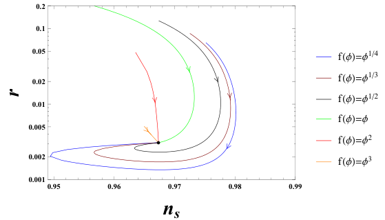
To show that the attractor (22) and (23) can be reached for arbitrary conformal factor $\Omega(\phi)=1+\xi f(\phi)$, we take $\omega(\phi)=1$, $n=2$, $\alpha=1$, and the power-law functions $f(\phi)=\phi^{k}$ with $k=1/4$, 1/3, 1/2, 1, 2 and 3. From Eqs. (22), (23) and (24), we get the attractor $n_{s}=0.9673$ and $r=0.0031$ for $N=60$. We vary the coupling constant $\xi$ and choose $N=60$ to calculate $n_{s}$ and $r$ for the models with the potential (21), and the results are shown in Fig. 1. From Fig. 1, we see that the attractor is reached in the strong coupling limit $\xi\gtrsim 100$.

Under the conformal transformation and the strong coupling condition (15), the potentials in the Jordan and Einstein frames have the relationship $V_{J}(\phi)=\Omega^{2}(\phi)U[\sqrt{3/2}\ln\Omega(\phi)]$. For any non-singular function $\Omega(\phi)$, these models will have the same observables $n_{s}$ and $r$ as those given by the potential $U(\psi)$ in Einstein frame. Therefore, these $\Omega(\phi)$ and $V_{J}(\phi)$ give the same attractors $n_{s}$ and $r$. By this method, we may get any attractor we want, and the existence of these $\xi$ attractors imposes a challenge to distinguish different models [20].

Acknowledgements: {acknowledgement} This research was supported in part by the National Natural Science Foundation of China under Grant No. 11475065.

References

- (1) R. Adam et al. (Planck), Astron. Astrophys. 594, A1 (2016), 1502.01582
- (2) P.A.R. Ade et al. (Planck), Astron. Astrophys. 594, A20 (2016), 1502.02114
- (3) A.A. Starobinsky, Phys. Lett. B. 91, 99 (1980)
- (4) L. Boubekeur, D. Lyth, JCAP 0507, 010 (2005), hep-ph/0502047
- (5) F.L. Bezrukov, M. Shaposhnikov, Phys. Lett. B 659, 703 (2008), 0710.3755
- (6) D.I. Kaiser, Phys. Rev. D 52, 4295 (1995), astro-ph/9408044
- (7) R. Kallosh, A. Linde, D. Roest, Phys. Rev. Lett. 112, 011303 (2014), 1310.3950
- (8) V. Mukhanov, Eur. Phys. J. C 73, 2486 (2013), 1303.3925
- (9) D. Roest, JCAP 1401, 007 (2014), 1309.1285
- (10) J. Garcia-Bellido, D. Roest, Phys. Rev. D 89, 103527 (2014), 1402.2059
- (11) L. Barranco, L. Boubekeur, O. Mena, Phys. Rev. D 90, 063007 (2014), 1405.7188
- (12) L. Boubekeur, E. Giusarma, O. Mena, H. Ramírez, Phys. Rev. D 91, 083006 (2015), 1411.7237
- (13) T. Chiba, Prog. Theor. Exp. Phys. 2015, 073E02 (2015), 1504.07692
- (14) P. Creminelli, S. Dubovsky, D. López Nacir, M. Simonović, G. Trevisan, G. Villadoro, M. Zaldarriaga, Phys. Rev. D 92, 123528 (2015), 1412.0678
- (15) R. Gobbetti, E. Pajer, D. Roest, JCAP 1509, 058 (2015), 1505.00968
- (16) J. Lin, Q. Gao, Y. Gong, Mon. Not. Roy. Astron. Soc. 459, 4029 (2016), 1508.07145
- (17) Q. Fei, Y. Gong, J. Lin, Z. Yi, JCAP (2017), 1705.02545
- (18) Q. Gao, Y. Gong (2017), 1703.02220
- (19) Q. Gao, Sci. China Phys. Mech. Astron. 60, 090401 (2017), 1704.08559
- (20) Z. Yi, Y. Gong, Phys. Rev. D 94, 103527 (2016), 1608.05922
- (21) A.D. Linde, Phys. Lett. B 129, 177 (1983)
- (22) R. Kallosh, A. Linde, JCAP 1310, 033 (2013), 1307.7938
- (23) J.J.M. Carrasco, R. Kallosh, A. Linde, Phys. Rev. D 92, 063519 (2015), 1506.00936