Vacuum energy of one-dimensional supercritical Dirac-Coulomb system
Abstract
Nonperturbative vacuum polarization effects are explored for a supercritical Coulomb source with in 1+1 D. Both the vacuum charge density and vacuum energy are considered. It is shown that in the overcritical region the behavior of vacuum energy could be significantly different from perturbative quadratic growth up to decrease reaching large negative values.
Keywords:
vacuum polarization, nonperturbative effects, critical charges, supercritical fields, one-dimensional H-like atomspacs
31.30.jf, 31.15-p, 12.20.-mI Introduction
Starting from Elliott and Loudon [1, 2], there is a lot of interest to the study of quasi-one-dimensional systems with Coulomb interaction, caused by the continuous growth of various physical applications [3, 4, 5, 6, 7, 8]. In this paper we explore the main nonperturbative features of a one-dimensional supercritical Dirac-Coulomb (DC) system. Whereas there is a lot of work devoted to such systems in 3+1 D (see, e.g., Refs. [9]-[13] and references therein), their 1+1 D analog has not been studied at all. Meanwhile, in Refs. [14]-[20], it was shown that in superstrong homogeneous magnetic fields the effective relativistic dynamics of the electronic component in H-like atoms turns out to be quasi-one-dimensional, while the first critical charge could be less than in absence of the field [17, 18, 19, 20].
A separate attention is drawn to nonperturbative vacuum polarization effects, caused by diving of discrete levels into lower continuum in supercritical static or adiabatically slow varying Coulomb fields [9, 10, 11, 12, 13]. This work explores such essentially nonperturbative vacuum effects for a model of supercritical DC system in one-dimensional case, with the main attention drawn to the vacuum polarization energy . Although the most of works consider the vacuum charge density as the main polarization observable, by means of which, in particular, the contribution of vacuum polarization to the Lamb shift is calculated, turns out to be not less informative and in many respects complementary to . Moreover, compared to , the main nonperturbative effects, which appear in vacuum polarization for due to levels diving into lower continuum, show up in the behavior of vacuum energy even more clear, demonstrating explicitly their possible role in the supercritical region.
For these purposes we consider here a simplified semi-analytic model with the external Coulomb source regulated via smooth cutoff at the scale [17, 27]
| (1) |
which allows to perform most part of calculations in analytical form, while the resulting qualitative picture turns out to be quite general.
As in other works on vacuum polarization in the strong Coulomb field [21, 22, 23, 24], radiative corrections from virtual photons are neglected. Henceforth, if it is not stipulated separately, relativistic units are used. Thence the electromagnetic coupling constant is also dimensionless, and numerical calculations, illustrating the general picture, are performed for .
II Vacuum Energy in Perturbative Approach for 1+1 D
In 1+1 D the expression for the regularized polarization operator , corresponding to the Feynman graph on Fig. 1, takes the form
| (2) | ||||

In particular, for
| (3) |
In the perturbative approach, the vacuum polarization energy to the leading order is given by
| (4) |
where is the external Coulomb source potential, which is assumed to be static, while is the vacuum density, determined from the polarization potential
| (5) |
The one-loop (Uehling) vacuum polarization potential is found from by means of the polarization function [25], namely
| (6) |
From (5) and (6) with account of (3) for the external Coulomb source (1) one obtains the following expression for the induced charge density (here and henceforth ):
| (7) | ||||
with and being the integral sine and cosine functions. From (4) via (7) one finds the lowest-order vacuum energy
| (8) | |||
From (7) it could be easily seen that within perturbation theory, the total induced vacuum charge vanishes
| (9) |
It would be worth-while to note, that although in this case the relation (9) is an obvious consequence of the explicit form of perturbative vacuum density (7), actually the status of the relation (9) turns out to be quite serious. Namely, it should be considered as a crush-test for the correct calculation of , since without nontrivial topology or asymptotics of the external field and/or some special boundary conditions in the subcritical region with the total induced charge should vanish [25, 26]. At the same time, for , due to nonperturbative effects, caused by discrete levels diving into lower continuum, the vacuum charge becomes nonzero [9, 10, 11, 13], and in what follows we will show how the latter circumstance shows up in the behavior of vacuum energy in the overcritical region.
III Wichmann-Kroll Contour Integration in 1+1 D
The most efficient nonperturbative approach to calculation of vacuum density is based on the Wichmann-Kroll (WK) method [21, 22, 23, 24] (see also Ref. [26] and references therein). The starting point of WK method is the following expression for the induced charge density:
| (10) |
where in such problems with external Coulomb source should be chosen at the threshold of the lower continuum, i.e. , while and are the eigenvalues and eigenfunctions of corresponding DC spectral problem.
The essence of WK method is that the vacuum density (10) can be calculated by means of the trace of the Green function for DC spectral problem, defined as
| (11) |
where it is convenient to take the Dirac matrices as , .
The formal solution of (11) should be written in the form
| (12) |
Following Refs. [21] and [22], the vacuum density is expressed via integration along contours and on the first sheet of the Riemann energy surface (Fig. 2)
| (13) |

Proceeding further, the trace of Green function is represented as
| (14) |
with , being the regular at solutions of DC problem, while is their Wronskian
| (15) |
It should be noted that actually is nothing else, but the Jost function of DC problem: the real-valued zeros of lie on the first sheet in the interval and coincide with discrete levels , while the complex ones reside on the second sheet with negative imaginary part of the wavenumber , and for give rise to elastic resonances.
To construct the Green function, let us consider first the DC spectral problem, which takes the form
| (16) |
with and being the upper and lower components of the Dirac wave function. For the potential (1) the system (16) has been considered in detail in Refs. [17] and [27]. Following Ref. [27], for the independent solutions of the Dirac equation are chosen in the form
| (17) |
where
| (18) | ||||
with , being the confluent hypergeometric functions of the first and second kinds correspondingly [28],
| (19) |
and should be chosen as such linear combinations of solutions (17), which are regular at and and connected through spatial inversion (with the latter being the direct consequence of parity conservation in the initial problem statement with external potential (1)):
| (20) | ||||
From the continuity condition at , one finds for the coefficients and
| (21) |
The Wronskian of solutions, which enters the expression for , takes the form
| (22) |
From (17)-(22) and (14) one finds the following expression for :
| (23) |
where by construction , while , which enters (23), equals to
| (24) |
In the next step one finds the asymptotics of on the arcs and in the upper half-plane (Fig. 2)
| (25) |
and on the arcs and in the lower half-plane
| (26) |
There follows from (25) and (26) that the integration along the contours and in (13) could be reduced to the imaginary axis (see Fig. 2), whence one finds the final expression for the vacuum charge density
| (27) |
In the case when there exist negative discrete levels with , instead of (27) one gets
| (28) |
Proceeding further, let us mention the general properties of under the change of the sign of external field and complex conjugation
| (29) |
and their direct consequence
| (30) |
There follows from (30), that is an odd function in and an even one in , whereas , on the contrary, is even in and odd in . Therefore, actually is determined via and so is definitely a real quantity, odd in . In the purely perturbative region, the representation of as an odd series in powers of external field follows directly from the Born series for Green function , whence
| (31) |
where is the free Green function. At the same time, in presence of negative discrete levels and, moreover, in the overcritical region with , the oddness in property of maintains [22], but now the dependence on external field cannot be described by a power series (31) any more, since there appear in certain additional, essentially nonperturbative, hence nonanalytic in components.
The expression for the vacuum density, given in (27) and (28), does not be automatically consistent with the requirement of total induced charge vanishing for . Moreover, it could be easily found from the explicit asymptotics of (25) and (26), that for behaves as , hence, the integral converges uniformly in . Proceeding further, one finds that, since for behaves like , the nonrenormalized decreases for as , and so the corresponding induced charge diverges logarithmically.
The general result, obtained in Ref. [22] via expansion of in powers of , and which is valid for any number of spatial dimensions, is that all the divergences of originate from the lowest-order graph (Fig. 1) only, while the next-to-leading orders are finite (see also Ref. [26] and references therein). So the calculation of renormalized vacuum density implies, that the terms of order should be extracted from the expression for (23) and replaced by (7). For these purposes, one finds first the component of the vacuum density , defined as
| (32) |
where and coincides with the first Born approximation . For the external source (1), the explicit form of reads
| (33) | ||||
with and being the integral exponent.
For the integral charge coming from vanishes. Without negative discrete levels, which prevent from analytic continuation, this statement can be proved via transition into the complex plane, where , represented through the converging integral , turns out to be an analytic function of with a cut, that appears from the Tricomi function in , and that could be always directed along the negative imaginary axis. So the integral induced charge can be expressed via contour integral along the arc of great circle in the upper half-plane. The latter vanishes exactly, what could be easily checked by direct calculation of the asymptotics . More concretely, the asymptotics of in the upper half-plane for takes the form
| (34) |
The leading term in the asymptotics (34) is purely imaginary, even in and odd in , and therefore disappears by integration over , the next-to-leading odd in term is canceled by , while the remaining terms vanish as . For the asymptotics is found from the reflection symmetry , and so on the whole great circle in the upper half-plane decreases uniformly as . This result confirms once more the conclusion, that all the divergences in originate from the terms linear in .
So the final answer for the renormalized induced charge density reads
| (35) |
where is the perturbative renormalized density (7), calculated via lowest-order diagram (Fig. 1). Such expression for provides vanishing of the total vacuum charge for . In presence of negative discrete levels, vanishing of the total charge for follows from model-independent arguments, based on the initial expression for the vacuum density (10). The latter means that any change of integral induced charge is possible for only, when certain discrete levels dive into lower continuum, and each diving level yields the change of integral charge by . Another way to achieve the same conclusion follows from the behavior of the integral over the imaginary axis , which enters the expressions (27) and (28) for , under such infinitesimal variation of external source, when the initially positive, infinitely close to zero level becomes negative. Then the corresponding pole of the Green function undergoes an infinitesimal displacement along the real axis and crosses zero too, what yields the change in equal to the residue at , namely, . So the integral induced charge, associated with , loses one unit, whenever there appears the next negative discrete level. Until this negative level exists, this loss of unit charge is compensated by the corresponding term, coming from the sum over negative discrete levels in (28). However, as soon as this level dives into lower continuum, the corresponding term in the sum over negative levels disappears, and so the total induced charge loses one unit of .
A more detailed picture of resulting changes in is similar to that considered in Refs. [9]–[11], [13], [25] for 3+1 D by means of Fano approach to the autoionization in atomic physics [29]. The main result is that whenever the level dives into lower continuum, the change in the vacuum density takes the form
| (36) |
It should be noted that this approach uses some approximations too, and so the expression (36) turns out to be exact only in the vicinity of corresponding . The correct way of calculation for all regions of should be based on relations (32) and (35) with subsequent control of expected integer value of the induced charge via direct integration of .

An illustration for such a picture is given in Figs. 3, 4 for in (1). Fig. 3 shows the renormalized vacuum density in the purely perturbative regime for , thereafter for , when the first is not reached yet, for , when the first (even) discrete level has just dived into lower continuum, afterwards for , when the second critical is not reached yet, and, finally, for , i.e. just after diving of the second (odd) discrete level into lower continuum. Herewith the direct numerical integration confirms that the total vacuum charge for equals to zero, for equals to , while for equals to , correspondingly. The critical charges are found from [27]
| (37) |
for even levels and
| (38) |
for odd.

Fig. 4 demonstrates that in the overcritical region with the changes of for increasing proceed not only in a step-like manner due to vacuum shell formations, originating from levels diving into lower continuum, but via permanent deformations in the density of states in both continua and evolution of discrete levels too. Namely, it displays the total changes in by transition through two first . The sum of vacuum density for and of two first discrete levels, taken at the threshold of the lower continuum, does not reproduce for no longer.
IV Nonperturbative Effects in Vacuum Energy for
Nonperturbative polarization effects, manifesting in for through formation of localized vacuum shells, give rise to corresponding nonperturbative changes in . As the formation of shells itself, this effect turns out to be essentially nonperturbative, but hitherto has not been considered in detail, since it was assumed that in the overcritical region the main contribution to should be produced by perturbative effects (see e.g. Ref. [11] and references therein). It should be specially marked that this effect cannot be evaluated directly via , since in the nonperturbative region there do not work neither (31), nor perturbative methods of restoration from . Let us also mention that the growth rate of the shells total number and the increase of the shell effect in with increasing depend very strongly on the number of spatial dimensions. In 1+1 D this rate is minimal, that is why the behavior of in the overcritical region depends not as much on shells, but on the renormalization term combined with degradation of the perturbative component in the nonrenormalized with increasing , what itself turns out to be an essentially nonperturbative effect.
The nonperturbative approach to vacuum energy calculation starts from the expression [9, 10, 11, 25]
| (39) |
which follows from the Dirac Hamiltonian, written in the invariant under charge conjugation form, and is defined up to the choice of the energy origin. In (39), even in absence of the external field, vacuum energy is negative and divergent. At the same time, the starting expression for the vacuum density (10) vanishes identically for . From this point of view, the most natural way is to normalize on the free case. Moreover, in the external fields like (1) there exists a (infinite) number of bound states. Therefore, in order to keep in the interaction effects only, the electron rest mass should be subtracted from the energy of each bound state. Thus, in physically motivated form the initial expression for should be written as
| (40) |
, defined in such a way, vanishes in absence of the external field, and so is in complete correspondence with the vacuum charge density (10).
Variation of with respect to leads to well-known Schwinger result in the form of vacuum charge density , combined with additional term, caused by the nonperturbative vacuum reconstruction for :
| (41) |
where with being the number of bound states, dived into lower continuum. yields a negative contribution to and has the form of a step-like function [11]. Whenever a discrete level reaches the lower continuum, one unit of the electron rest mass is lost by the vacuum energy via . Such fixed negative jumps in the vacuum energy are treated as indication on phase transition from the neutral vacuum into the charged one, which turns out to be the ground state of the electron-positron field in supercritical Coulomb fields [9, 10, 11, 13, 25].
In the next step (40) should be divided into separate contributions from discrete and continuous spectra, applying to the difference of integrals over the continuous spectrum the well-known tool, which represents this difference in the form of an integral from the elastic scattering phase . Such technique has been used quite effectively in calculation of one-loop quantum corrections to the soliton mass in essentially nonlinear field-theoretic models in 1+1 D (see Refs. [30] and [31] and references therein). Upon dropping certain almost obvious intermediate steps, the final answer reads
| (42) |
where is the sum of phase shifts for the given wavenumber from electron and positron scattering states of both parities.
Such approach to calculation of turns out to be quite effective, since behaves much better, than each of elastic phases separately, both in IR and UV limits, and turns out to be automatically an even function of the external field. Moreover, in 1+1 D, for the Coulomb potentials like (1), the vacuum energy, taken in the form (42), turns out to be finite without any special UV-renormalization. As it will be shown by direct calculation below, is finite for and behaves like for , hence, the phase integral in (42) is always convergent. In turn, the total bound energy of discrete levels is also finite, since behave like for . However, the convergence of after subtraction (40) does not mean any hidden UV-renormalization, rather it is caused exclusively by specifics of 1+1 D. Although the subtraction (40) should be implemented under suitable intermediate UV-regularization, actually it is nothing else, but the choice of pertinent reference frame for . The need in renormalization of via the lowest-order diagram (Fig. 1) follows from the analysis of , performed in the preceding section. The latter shows that without such genuine UV-renormalization the induced charge does not acquire the value that should be expected from general grounds [25, 26]. Another requirement is that for the answer for should coincide with the perturbative result , found from (4)-(8). Since for the connection between and is described by perturbative relations (4)-(6), it is easy to verify that nonrenormalized does not satisfy this condition. With more details this question is explored below in terms of the renormalization coefficient (44).
Thus, in the way quite similar to , we should pass from to the renormalized vacuum energy . In the form, well-adapted for practical use, could be represented as
| (43) |
where
| (44) |
while the renormalization coefficient depends solely on the profile of the external Coulomb field and, depending on the parameters of the source, could be of arbitrary sign, as well as negligibly small (see below).
Now let us consider the calculation of for the Coulomb source of the form (1). For these purposes, the spinor components of solutions of the Dirac equation in the upper and lower () continua for should be chosen in the following form
| (45) | ||||
where
| (46) |
The relations for coefficients are derived from the conditions of even or odd continuation of solutions (45) to negative half-axis . As a result, for even solutions
| (47) |
while for odd
| (48) |
The solutions of Dirac equation for the discrete spectrum () for should be written as
| (49) | ||||
where and are defined as in (19). Discrete levels are found from the condition for combined with for even levels and for odd, what gives the equation
| (50) |
for even levels, and
| (51) |
for odd.
Separate phase shifts are found from the asymptotics of solutions (45) for and contain Coulomb logarithms , which in the total phase
| (52) |
cancel each other, so in (52) for separate phases only the regular at part should be kept, namely
| (53) |
where , , and . The phases (53) contain for the logarithmic terms , which cancel each other again, and so there remains in the asymptotics of only the regular part, decreasing . More concretely, the UV-asymptotics of takes the form
| (54) |
It should be mentioned that the calculation of (54) for reasonable time could be performed by means of symbolic computer algebra only. is finite for as well, since all the singular terms in the IR-asymptotics for even and for odd in the upper and lower continua phases cancel as well. The exact IR-asymptotics for is found by means of Taylor representation for confluent hypergeometric functions [28] and reads
| (55) | |||
where
| (56) | ||||
In the considered range of external source parameters, the value of is uniquely determined through expressions (55)–(56) and lies always in the interval , what could be checked numerically via explicit restoration of on the whole half-line , starting from UV-asymptotics (54). The behavior of as a function of is shown in Fig. 5.

The typical behavior as a function of wavenumber is shown in Fig. 6 for . For such a size of external source the critical charge for the first even level amounts to , therefore for (Fig. 6a) the overcritical region is not reached yet, and so reveals a smooth behavior on the whole half-line . For (Fig. 6b) the first even level has already dived into lower continuum, thence, there appears in the phase the first and yet sufficiently narrow elastic (positron) resonance. The origin and features of such resonances in the overcritical region are caused by evolution of the Green function poles, corresponding to discrete levels, into second sheet of the Riemann energy surface after achieving the threshold of lower continuum (the beginning of left cut on Fig. 2), and have been discussed in detail in Refs. [9]–[11], [13], [25]. To demonstrate the displacement and broadening of resonances with increasing , Fig. 6c shows for : two first resonances, which appear after achieving the lower continuum by the first even () and first odd () discrete levels, become already sufficiently less pronounced, while the second even level () has just dived into the lower continuum, the corresponding pole lies very close to the beginning of the left cut and shows up in the phase as an extremely narrow low-energy resonance.
![[Uncaptioned image]](1709.04239v1/phaseZ=115.png)
a)
![[Uncaptioned image]](1709.04239v1/phaseZ=117.png)
b)

c)
As a result, in (42) both the phase integral and the total bound energy of discrete levels converge without any additional regularization of Coulomb asymptotics of external potential for , and so can be evaluated by means of standard numerical recipes. It should be mentioned also that actually the UV-asymptotics (54) of is valid for . This circumstance plays a significant role in calculation of the phase integral in (42), since it allows for a substantial simplification of integration for asymptotically large .
Now let us specify the main nonperturbative effects in the behavior of phase integral and total bound energy in (42) for the overcritical region. As it follows from Fig. 5, oscillates in limits , and so each subsequent resonance gives rise to negative jump of the phase equal to , thereafter increases smoothly by again. As a result, after emergence of the next resonance, phase integral acquires a certain negative jump of the derivative, and so becomes an oscillating and smoothly decreasing function of . On the contrary, discrete levels bound energy grows continuously with , since there grows with the bound energy of each level, except , when the corresponding level dives into lower continuum and there appears a jump of bound energy equal to . Moreover, in 1+1 D it is indeed the total bound energy, that dominates in in the overcritical region before renormalization, rather than the phase integral, which gives in a significantly less contribution. Such behavior of the phase integral and is a peculiar feature of 1+1 D.
The next factor, affecting the behavior of in , is the renormalization term in (43). Moreover, in 1+1 D this contribution in turns out to be the dominant one in the overcritical region, since the sum of discrete levels and so the non-renormalized grows in this region . At the same time, the number of dived levels, hence the number of vacuum shells, increase , but the correlation between and is not simple, since the relation between and in the overcritical region is essentially nonlinear.
For the external source like (1), there follows directly from the definition of (44) and dimensional arguments that the asymptotics of for both and should be . For more details, let us represent as
| (57) |
where originates from perturbative polarization energy , found in (8),
| (58) |
while comes from the Born term for (31), (33)
| (59) | ||||
In (59), in the first term the integration over is performed, while in the second term it is also possible, but the result contains an additional integration, and so in what follows it will be employed in the limit only.
Let us start with the asymptotics for . For these purposes, should be divided in following parts:
| (60) | ||||
with being the Euler’s constant.
The first term in (60) equals to . Here it should be noted that the integral
cannot be evaluated analytically (at least the authors did not succeed in searching for the answer in open sources), but the numerical calculation unambiguously indicates that its value is .
The second term in is explored by taking account of
thereafter it can be rewritten as
| (61) | ||||
Again, the integrals over , entering (61), cannot be found analytically, but the numerical calculation says that they are equal to and , correspondingly. So (61) reduces to
| (62) |
In the next step, it could be easily verified that the last term in vanishes for . So the nonvanishing terms in the asymptotics of for can be represented as
| (63) |
Now let us consider . For these purposes in the first integral in (59), the integration region should be divided into two pieces and . In the first region , the arguments of exponents does not exceed 1, thence, upon expanding the exponents into power series and extracting from the leading terms in , one finds that the main contribution to the integral comes from the latter terms only, while the others vanish for . Thereafter the integral can be calculated analytically and for equals to
| (64) |
In the second region for , the integration is performed over asymptotically large only, therefore the integral can be evaluated as
| (65) |
The integral over converges, and so the contribution from the second region behaves for .
Evaluation of the second integral in for gives
| (66) |
As a result, the nonvanishing terms in for are
| (67) |
Finally, for the nonvanishing part of takes the form
| (68) |
It should be noted that (68) works quite well already for .
For it could be easily found, that , while in the expansion of in the inverse powers of the argument
should be used. Whence it follows that in the first integral in (59), the expansion starts from , and so it turns out to be also. In the second integral the expansion begins with , what upon integration over yields the leading term equal to . Thus, for one obtains
| (69) |
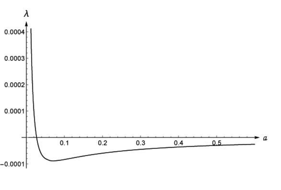
From (68) and (69) one immediately finds that , when considered on the whole half-line , changes its sign and so should possess at least one zero. The behavior of in the intermediate region between the asymptotics is shown in Fig. 7. As expected, acquires one zero at , what corresponds to the “size” of the Coulomb source fm.
Now let us explore the role of in . If , then for the renormalization coefficient is positive and sufficiently large, and there dominates in the increasing -component. At the same time, for the renormalization coefficient falls rapidly into negative region, and so the term in becomes a decreasing one. That is why for there appears the effect of decreasing vacuum energy up to large negative values, since the nonrenormalized grows in the overcritical region slower than . For , the answer depends on the interplay between nonperturbative effects in the phase integral, which try to decrease the vacuum energy, and the bound energy of discrete spectrum, which acts in the opposite direction. So should significantly depend on the concrete form of the external potential. In the considered case, the contribution of the discrete spectrum dominates, hence increases, but it grows no longer square, but more slowly, namely .
This general picture correlates completely with concrete calculations, performed for a wide range of external field parameters. In Figs. 8a-d the behavior of is shown for . The number of shells for these values of is estimated as , correspondingly. For the renormalization parameter , hence the vacuum energy as a function of shows up a square growth, at first due to perturbative effects, and further for due to . For the renormalization term disappears, and so the dominant contribution in for comes from the discrete levels bound energy, which (without jumps) behaves . For , on the contrary, and correspondingly, the nonrenormalized (without jumps) are estimated as and . Therefore, due to negative quadratic renormalizing term, reveals a decrease up to substantial negative values. Herewith it is clearly visible in Figs. 8c,d that there takes place first a square growth, caused by perturbative effects, which for degrade under scenario described above, while the main contribution comes from the renormalization term and so decreases almost quadratically.
![[Uncaptioned image]](1709.04239v1/E_vac_a=001_0-200.png)
a)
![[Uncaptioned image]](1709.04239v1/Evp_eta=0_a=0,027.png)
b)

c)

d)
![[Uncaptioned image]](1709.04239v1/PhaseInt_a=cr.png)
a)
![[Uncaptioned image]](1709.04239v1/Details1_a=cr.png)
b)

c)
![[Uncaptioned image]](1709.04239v1/PhaseInt_a=1.png)
a)
![[Uncaptioned image]](1709.04239v1/Details1_a=1.png)
b)

c)
With more details, the formation of resulting curves for looks as follows. The most representative cases here turn out to be and . For the first one, the behavior of ingredients of the final answer is shown in Fig. 9. Fig. 9a shows the behavior of the phase integral. As expected, the latter is an oscillating function of with negative jumps of the derivative at . Fig. 9b includes the nonrenormalized (solid line), the total bound energy (dashed), the phase integral (dash-dotted) and the number of shells (dotted). As it was mentioned above, the magnitude of phase integral is much smaller compared to the total discrete levels bound energy, and so the curves of the latter and are almost indistinguishable. Fig. 9c shows the renormalized (solid line) and its approximation (dashed), formed by the function , which simulates the nonrenormalized without jumps at , and jumps by (-1) at . Figs. 10a,b,c repeats the same details of formation for . The main difference here is that the approximation of is formed now by the function plus renormalization term and jumps at . Note also that the behavior of the number of shells is quite different. For the first is much less, than for , but for the number of shells increases for more rapidly compared to .

a)

b)

c)

d)
V Conclusion
To conclude let us firstly mention that the calculation of vacuum energy could be made completely self-consistent by means of (42)–(44) combined with the lowest-order diagram renormalization without applying to the vacuum density and effects of shells. However, in fact the decrease of in the overcritical region is caused indeed by the nonperturbative changes in the vacuum density for due to discrete levels diving into lower continuum. In 1+1 D, due to specifics of one-dimensional DC problem, the growth of vacuum shells number , at least for the considered range of external sources. Therefore, they are able only to decrease the speed of growth of nonrenormalized in the overcritical region up to , , and so the dominant contribution comes from the renormalization term . In more spatial dimensions, the shell effect turns out to be much more pronounced. Such behavior of in the overcritical region confirms the assumption of the neutral vacuum transmutation into the charged one under such conditions [9, 10, 11, 13, 25], and thereby of spontaneous positron emission, accompanying the emergence of the next vacuum shell due to total charge conservation.
It would be worthwhile to note that as in other works on vacuum polarization under strong Coulomb field [21, 22, 23, 24], here the contribution of virtual photons was ignored, and so only the one-loop diagram (Fig. 1) has been used for vacuum energy evaluation. A simple estimate of the effects, coming from virtual photons exchange, could be based on Coulomb energy, associated with the vacuum charge density, with the same cutoff, as in the external field (1)
| (70) |
Evaluation of shows that at this assessment of one-photon exchange contribution to the vacuum energy the effect turns out to be sufficiently small, about two orders less than that from the fermion loop (see Fig. 11). Figs. 11a,b shows as a function of in comparison with , found via (42)–(44), for . Figs. 11c,d demonstrate as a function of for . for these values of the cutoff are already given on Fig. 8c,d. Note also that in vacuum effects, caused by virtual photons, the shell effect shows up quite clearly.
Thus, in 1+1 D vacuum polarization effects could yield for pertinent parameters of Coulomb sources such behavior of the vacuum energy in the overcritical region that is significantly different from the perturbative one. The specifics of 1+1 D shows up here in that the decrease rate of in the considered range of Coulomb sources does not exceed , due to extremely slow increase of vacuum shells number in one-dimensional case. Herewith, for obvious reasons, we omit the question of to what extent such a supercritical region could be physically realizable (as well as the whole one-dimensional picture for a relativistic H-like atom itself).
References
- [1] R. Loudon, “One-dimensional hydrogen atom,” Am. J. Phys., vol. 27, no. 9, pp. 649–655, 1959.
- [2] R. Elliott and R. Loudon, “Theory of the absorption edge in semiconductors in a high magnetic field,” J. Phys. Chem. Solids, vol. 15, no. 3-4, pp. 196–207, 1960.
- [3] M. M. Nieto, “Electrons above a helium surface and the one-dimensional rydberg atom,” Phys. Rev. A, vol. 61, no. 3, p. 034901, 2000.
- [4] A. López-Castillo and C. R. de Oliveira, “Classical ionization for the aperiodic driven hydrogen atom,” Chaos, Solitons & Fractals, vol. 15, no. 5, pp. 859–869, 2003.
- [5] F. Essler, F. Gebhard, and E. Jeckelmann, “Excitons in one-dimensional mott insulators,” Phys. Rev. B, vol. 64, no. 12, p. 125119, 2001.
- [6] F. Wang, Y. Wu, M. S. Hybertsen, and T. F. Heinz, “Auger recombination of excitons in one-dimensional systems,” Phys. Rev. B, vol. 73, no. 24, p. 245424, 2006.
- [7] X. Guan, B. Li, and K. Taylor, “Strong parallel magnetic field effects on the hydrogen molecular ion,” J. Phys. B, vol. 36, no. 17, p. 3569, 2003.
- [8] H. Ruder, G. Wunner, H. Herold, and F. Geyer, Atoms in Strong Magnetic Fields: Quantum Mechanical Treatment and Applications in Astrophysics and Quantum Chaos. Springer Science & Business Media, 2012.
- [9] J. Reinhardt and W. Greiner, “Quantum electrodynamics of strong fields,” Rep. Prog. Phys., vol. 40, no. 3, p. 219, 1977.
- [10] W. Greiner, B. Muller, W. Greiner, and J. Rafelski, Quantum electrodynamics of strong fields. Springer-Verlag Berlin-Heidelberg, 1985.
- [11] G. Plunien, B. Muller, and W. Greiner, “The casimir effect,” Phys. Rep., vol. 134, no. 2, pp. 87–193, 1986.
- [12] V. M. Kuleshov, V. D. Mur, N. B. Narozhny, A. M. Fedotov, Y. E. Lozovik, and V. S. Popov, “Coulomb problem for a nucleus,” Phys. Usp., vol. 58, no. 8, p. 785, 2015.
- [13] J. Rafelski, J. Kirsch, B. Müller, J. Reinhardt, and W. Greiner, “Probing qed vacuum with heavy ions,” in New Horizons in Fundamental Physics, pp. 211–251, Springer, 2017.
- [14] R. Barbieri, “Hydrogen atom in superstrong magnetic fields: Relativistic treatment,” Nucl. Phys. A, vol. 161, no. 1, pp. 1–11, 1971.
- [15] A. E. Shabad and V. V. Usov, “Positronium collapse and the maximum magnetic field in pure qed,” Phys. Rev. Lett., vol. 96, no. 18, p. 180401, 2006.
- [16] A. Shabad and V. Usov, “Bethe-salpeter approach for relativistic positronium in a strong magnetic field,” Phys. Rev. D, vol. 73, no. 12, p. 125021, 2006.
- [17] V. Krainov, “Hydrogen-like atom in a super-strong magnetic field,” JETP, vol. 64, no. 3, pp. 800–803, 1973.
- [18] V. Oraevskii, A. Rex, and V. Semikoz, “Spontaneous production of positrons by a coulomb center in a homogeneous magnetic field,” JETP, vol. 45, p. 428, 1977.
- [19] B. Karnakov and V. Popov, “A hydrogen atom in a superstrong magnetic field and the zeldovich effect,” JETP, vol. 97, no. 5, pp. 890–914, 2003.
- [20] M. I. Vysotskii and S. I. Godunov, “Critical charge in a superstrong magnetic field,” Phys. Usp., vol. 184, no. 2, pp. 206–210, 2014.
- [21] E. H. Wichmann and N. M. Kroll, “Vacuum polarization in a strong coulomb field,” Phys. Rev., vol. 101, no. 2, p. 843, 1956.
- [22] M. Gyulassy, “Higher order vacuum polarization for finite radius nuclei,” Nucl. Phys. A, vol. 244, no. 3, pp. 497–525, 1975.
- [23] L. S. Brown, R. N. Cahn, and L. D. McLerran, “Vacuum polarization in a strong coulomb field. i. induced point charge,” Phys. Rev. D, vol. 12, no. 2, p. 581, 1975.
- [24] A. Neghabian, “Vacuum polarization for an electron in a strong coulomb field,” Phys. Rev. A, vol. 27, no. 5, p. 2311, 1983.
- [25] W. Greiner and J. Reinhardt, Quantum electrodynamics. Springer Science & Business Media, 2012.
- [26] P. J. Mohr, G. Plunien, and G. Soff, “Qed corrections in heavy atoms,” Phys. Rep., vol. 293, no. 5-6, pp. 227–369, 1998.
- [27] K. A. Sveshnikov and D. I. Khomovskii, “Schrödinger and dirac particles in quasi-one-dimensional systems with a coulomb interaction,” Theor. Math. Phys., vol. 173, no. 2, pp. 1587–1603, 2012.
- [28] H. Bateman and A. Erdélyi, Higher trascendental functions. The Gamma function. The hypergeometric function. Legendre functions. Vol. 1. McGraw-Hill, 1953.
- [29] U. Fano, “Effects of configuration interaction on intensities and phase shifts,” Phys. Rev., vol. 124, no. 6, p. 1866, 1961.
- [30] R. Rajaraman, “Instantons and solitons,” 1982.
- [31] K. Sveshnikov, “Dirac sea correction to the topological soliton mass,” Phys. Lett. B, vol. 255, no. 2, pp. 255–260, 1991.