One-Bit Sphere Decoding for Uplink Massive MIMO Systems with One-Bit ADCs

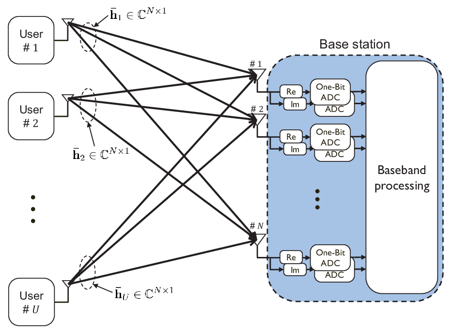
We consider an uplink massive MIMO system in which $U$ uplink users, each equipped with a single transmit antenna, send data symbols to a BS equipped with $N$ receive antennas, as illustrated in Fig. 1. We denote a (data) symbol vector sent by the uplink users at time slot $t$ as ${\bf\bar{x}}[t]=[{\bar{x}}_{1}[t],{\bar{x}}_{2}[t],\cdots,{\bar{x}}_{U}[t]]^{\top}\in\mathbb{C}^{U}$, where each data symbol ${\bar{x}}_{u}[t]$ is drawn from a constellation set $\mathcal{\bar{X}}$ with size $M$, i.e., $|\mathcal{\bar{X}}|=M$, and satisfies $\mathbb{E}[|{\bar{x}}_{u}[t]|^{2}]=1$. In other words, the symbol vector ${\bf\bar{x}}[t]$ collects the transmitted signals from all users at time slot $t$. We define $\mathcal{X}$ as a constellation set for real or imaginary part such that $\mathcal{\bar{X}}=\{x_{\rm R}+jx_{\rm I}~|~x_{\rm R},x_{\rm I}\in\mathcal{X}\}$ and $|\mathcal{X}|=\sqrt{M}$. Then $\mathcal{X}^{2U}$ represents a symbol vector set that contains all possible combinations of transmit symbols sent by the $U$ uplink users.

We assume a frequency-flat MIMO channel. Let ${\bf\bar{h}}_{u}\in\mathbb{C}^{N\times 1}$ be the channel vector from the $u$th uplink user to the BS. Then, the channel impulse response is given by a channel matrix ${\bf\bar{H}}=[{\bf\bar{h}}_{1},\ldots,{\bf\bar{h}}_{U}]\in\mathbb{C}^{N\times U}$. We also make two assumptions: 1) perfect synchronization at the BS and 2) perfect power control across all uplink users. Under these assumptions, the received signal vector at time slot $t$ before ADC quantization is

$\displaystyle{\bf\bar{r}}[t]={\bf\bar{H}}{\bf\bar{x}}[t]+{\bf\bar{z}}[t]\in\mathbb{C}^{N},$

(1)

where ${\bf\bar{z}}[t]=[{\bar{z}}_{1}[t],{\bar{z}}_{2}[t],\cdots,{\bar{z}}_{N}[t]]^{\top}$ has elements independently drawn from a complex Gaussian distribution with zero mean and variance $\sigma^{2}$. We assume a block fading model in which the channel is time-invariant during coherence time interval. We denote $T_{\rm d}$ as the duration (the number of time slots) for data detection. The complex received signal in (1) can be equivalently rewritten in a real-form as

$\displaystyle\underbrace{\left[{\begin{array}[]{c}{\rm Re}({\bf\bar{r}}[t])\\ {\rm Im}({\bf\bar{r}}[t])\\ \end{array}}\right]}_{{\bf r}[t]}=\underbrace{\left[{\begin{array}[]{cc}{\rm Re}({\bf\bar{H}})&-{\rm Im}({\bf\bar{H}})\\ {\rm Im}({\bf\bar{H}})&{\rm Re}({\bf\bar{H}})\\ \end{array}}\right]}_{{\bf H}}\underbrace{\left[{\begin{array}[]{c}{\rm Re}({\bf\bar{x}}[t])\\ {\rm Im}({\bf\bar{x}}[t])\\ \end{array}}\right]}_{{\bf x}[t]}+\underbrace{\left[{\begin{array}[]{c}{\rm Re}({\bf\bar{z}}[t])\\ {\rm Im}({\bf\bar{z}}[t])\\ \end{array}}\right]}_{{\bf z}[t]},$

where ${\rm Re}({\bf A})$ and ${\rm Im}({\bf A})$ denote the real and complex parts of a complex matrix ${\bf A}$, respectively.

We consider the use of one-bit ADCs at each receive antenna, which implies that the real and the imaginary components of the received signal are separately quantized to binary levels. In this paper, ${\rm sign}(\cdot)$ is the quantization function, which essentially maps a positive value to 1 and a negative value to -1. Then the received signal after the ADCs at time slot $t$ is defined as ${\bf y}[t]=\left[y_{1}[t],y_{2}[t]\cdots,y_{2N}[t]\right]^{\top}\in\{+1,-1\}^{2N}$ with

$\displaystyle{y}_{i}[t]={\rm sign}({r}_{i}[t])={\rm sign}\left({\bf h}_{i}^{\top}{\bf x}[t]+{z}_{i}[t]\right),$

(10)

for all $i\in\mathcal{I}=\{1,2,\ldots,2N\}$, where ${\bf h}_{i}^{\top}$ is the $i$-th row of the channel matrix ${\bf H}$, and $z_{i}[t]$ is the $i$-th element of ${\bf z}[t]$.

We provide some definitions that will be used in the sequel.

Definition 1 (Codewords and codebook [13, 14]): We define ${\bf c}_{k}={\rm sign}({\bf H}{\bf x}_{k})\in\{-1,1\}^{2N}$ as the $k$-th (binary) codeword vector corresponding to the $k$-th symbol vector ${\bf x}_{k}\in\mathcal{X}^{2U}$. For $k\in\mathcal{K}=\big\{1,2,\ldots,K=M^{U}\big\}$, each codeword vector ${\bf c}_{k}={\rm sign}({\bf H}{\bf x}_{k})$ can be interpreted as a noise-free received signal when a symbol vector ${\bf x}_{k}\in\mathcal{X}^{2U}$ is transmitted via the channel matrix ${\bf H}$. We also define a codebook by a collection of codeword vectors, i.e., $\mathcal{C}=\{{\bf c}_{1},{\bf c}_{2},\ldots,{\bf c}_{K}\}$. Note that similar notions for the codeword vectors and the codebook are considered in [13, 14].

Definition 2 (Weighted Hamming distance between codewords): Let ${\bf c}_{k}=[c_{k,1},c_{k,2},\cdots,c_{k,2N}]^{\top}$ and ${\bf c}_{j}=[c_{j,1},c_{j,2},\cdots,c_{j,2N}]^{\top}$ be binary codeword vectors in a codebook $\mathcal{C}$. In addition, let ${\bf w}=[w_{1},w_{2},\cdots,w_{2N}]^{\top}\in\mathbb{R}^{2N}$ and ${\bf\tilde{w}}=[{\tilde{w}}_{1},{\tilde{w}}_{2},\cdots,{\tilde{w}}_{2N}]^{\top}\in\mathbb{R}^{2N}$ be weight vectors that consist of positive elements. The weight vector ${\bf w}$ is assigned when measuring the distance between the elements of ${\bf c}_{k}$ and ${\bf c}_{j}$ that have different signs. Whereas, the weight vector ${\bf\tilde{w}}$ is assigned when measuring the distance between the elements of ${\bf c}_{k}$ and ${\bf c}_{j}$ that have the same sign. Then, the weighted Hamming distance between ${\bf c}_{k}$ and ${\bf c}_{j}$ with respect to ${\bf w}$ and ${\bf\tilde{w}}$ is defined as

$\displaystyle d_{\rm w}({\bf c}_{k},{\bf c}_{j};{\bf w},{\bf\tilde{w}})\!=\!\sum_{i=1}^{2N}w_{i}\|c_{k,i}\!-\!c_{j,i}\|_{0}\!+\!\!\sum_{i=1}^{2N}{\tilde{w}}_{i}(1-\|c_{k,i}\!-\!c_{j,i}\|_{0}),$

(11)

where $\|{\bf a}\|_{0}$ is the zero norm that denotes the number of nonzero elements in a vector ${\bf a}$. Note that when ${\tilde{w}}_{i}>0$ for any $i$, the weighted Hamming distance between two same codewords can be non-zero.

We present the MLD for uplink multi-user MIMO systems with one-bit ADCs that was originally introduced in [17]. Let $p\left({\bf y}[t]|{\bf x}_{k}\right)$ be the likelihood function with the received signal ${\bf y}[t]$ when the $k$-th symbol vector, ${\bf x}_{k}\in\mathcal{X}^{2U}$, was sent at time slot $t$. Then, $p\left({\bf y}[t]|{\bf x}_{k}\right)$ is given by [17]

$\displaystyle p\left({\bf y}[t]|{\bf x}_{k}\right)$

$\displaystyle=\prod_{i=1}^{2N}p\left({y}_{i}[t]|{\bf x}_{k}\right)=\prod_{i=1}^{2N}\left(1-Q\left(\sqrt{\frac{2}{\sigma^{2}}}y_{i}[t]{\bf h}_{i}^{\top}{\bf x}_{k}\right)\right),$

(12)

where $Q(x)=\int_{x}^{\infty}\frac{1}{\sqrt{2\pi}}e^{-\frac{t^{2}}{2}}{\rm d}t$ is a standard Q-function. Using (12), MLD for a MIMO system with one-bit ADCs is represented by the following optimization problem:

	$\displaystyle{\bf\hat{x}}_{\rm MLD}[t]$	$\displaystyle=\underset{{\bf x}_{k}\in\mathcal{X}^{2U}}{\operatornamewithlimits{argmax}}~p\left({\bf y}[t]|{\bf x}_{k}\right)$		(13)
		$\displaystyle=\underset{{\bf x}_{k}\in\mathcal{X}^{2U}}{\operatornamewithlimits{argmax}}~\prod_{i=1}^{2N}\left(1-Q\left(\sqrt{\frac{2}{\sigma^{2}}}y_{i}[t]{\bf h}_{i}^{\top}{\bf x}_{k}\right)\right).$		(14)

We show that the MLD is equivalent to MWD. To this end, we demonstrate that the log-likelihood function can be rewritten in the form of the weighted Hamming distance in (11). Let $\mathcal{N}_{k}^{\rm e}[t]=\{i:y_{i}[t]\neq c_{k,i}\}$ be the index set of the received signal elements that have different signs with the elements of the $k$-th codeword vector under the premise that ${\bf x}_{k}\in\mathcal{X}^{2U}$ was sent at time slot $t$. Using this index set, we rewrite the likelihood function in (12) as

$\displaystyle{p}\left({\bf y}[t]|{\bf x}_{k}\right)$

$\displaystyle=\prod_{i\in\mathcal{N}_{k}^{\rm e}[t]}Q\left(-\sqrt{\frac{2}{\sigma^{2}}}y_{i}[t]{\bf h}_{i}^{\top}{\bf x}_{k}\right)\prod_{i\notin\mathcal{N}_{k}^{\rm e}[t]}\left(1-Q\left(\sqrt{\frac{2}{\sigma^{2}}}y_{i}[t]{\bf h}_{i}^{\top}{\bf x}_{k}\right)\right),$

(15)

where the equality is obtained by applying the property of the Q-function: $Q(x)=1-Q(-x)$. Then we take the logarithm of (15) which yields

$\displaystyle\ln\left(p\left({\bf y}[t]|{\bf x}_{k}\right)\right)$

$\displaystyle=\sum_{i\in\mathcal{N}_{k}^{\rm e}[t]}\ln Q\left(-\sqrt{\frac{2}{\sigma^{2}}}y_{i}[t]{\bf h}_{i}^{\top}{\bf x}_{k}\right)+\sum_{i\notin\mathcal{N}_{k}^{\rm e}[t]}\ln\left(1-Q\left(\sqrt{\frac{2}{\sigma^{2}}}y_{i}[t]{\bf h}_{i}^{\top}{\bf x}_{k}\right)\right).$

(16)

To simplify, we define two weights $w_{k,i}^{\prime}$ and ${\tilde{w}}_{k,i}^{\prime}$ as

$\displaystyle w_{k,i}^{\prime}\triangleq-\ln Q\left(-\sqrt{\frac{2}{\sigma^{2}}}y_{i}[t]{\bf h}_{i}^{\top}{\bf x}_{k}\right)>0,$

(17)

and

$\displaystyle{\tilde{w}}_{k,i}^{\prime}\triangleq-\ln\left(1-Q\left(\sqrt{\frac{2}{\sigma^{2}}}y_{i}[t]{\bf h}_{i}^{\top}{\bf x}_{k}\right)\right)>0.$

(18)

Using these weights, the log-likelihood function in (16) can be expressed as

	$\displaystyle\ln\left(p\left({\bf y}[t]|{\bf x}_{k}\right)\right)$	$\displaystyle=-\sum_{i\in\mathcal{N}_{k}^{\rm e}[t]}w_{k,i}^{\prime}-\sum_{i\notin\mathcal{N}_{k}^{\rm e}[t]}{\tilde{w}}_{k,i}^{\prime}$
		$\displaystyle=-\sum_{i=1}^{2N}{w}_{k,i}^{\prime}\left\|{y}_{i}[t]-c_{k,i}\right\|_{0}-\sum_{i=1}^{2N}{\tilde{w}}_{k,i}^{\prime}(1-\left\|{y}_{i}[t]+c_{k,i}\right\|_{0}),$		(19)

where the last equality holds because

$\displaystyle\left\|{y}_{i}[t]-c_{k,i}\right\|_{0}=\begin{cases}1,&i\in\mathcal{N}_{k}^{\rm e}[t],\\ 0,&i\notin\mathcal{N}_{k}^{\rm e}[t].\\ \end{cases}$

From Definition 2 in Section II-B, the log-likelihood function is expressed in the form of the weighted Hamming distance:

$\displaystyle\ln\left(p\left({\bf y}[t]|{\bf x}_{k}\right)\right)$

$\displaystyle=-d_{\rm w}\left({\bf y}[t],{\bf c}_{k};{\bf w}_{k}^{\prime},{\bf\tilde{w}}_{k}^{\prime}\right).$

(20)

By applying the result in (20) to the definition of MLD, we can show that the MWD is equivalent to the MLD:

$\displaystyle{\bf\hat{x}}_{\rm MLD}[t]=\underset{{\bf x}_{k}\in\mathcal{X}^{2U}}{\operatornamewithlimits{argmax}}~\ln\left(p\left({\bf y}[t]|{\bf x}_{k}\right)\right)=\underset{{\bf x}_{k}\in\mathcal{X}^{2U}}{\operatornamewithlimits{argmin}}~d_{\rm w}\left({\bf y}[t],{\bf c}_{k};{\bf w}_{k}^{\prime},{\bf\tilde{w}}_{k}^{\prime}\right).$

(21)

Based on the MLD representation in (21), we develop a new MWD method that provides a near-MLD solution. The key idea of the developed MWD is to use closed-form weight vectors that tightly approximate the weight vectors in (21). In this approximation, we adopt a Q-function approximation in [27] which demonstrates that ${\hat{Q}}(x)=\frac{1}{2}e^{-0.374x^{2}-0.777x}$ tightly approximates the Q-function for non-negative $x$ with the absolute error less than $10^{-3}$, i.e.,

$\displaystyle|Q(x)-{\hat{Q}}(x)|\leq 10^{-3},~\text{for}~x\geq 0.$

(22)

By applying $Q(x)\approx\frac{1}{2}e^{-0.374x^{2}-0.777x}$ for $x\geq 0$ to both (17) and (18), we obtain two closed-form weights $w_{k,i}$ and $w_{k,i}^{\prime}$ that approximate the original weights ${w}_{k,i}^{\prime}$ and ${\tilde{w}}_{k,i}^{\prime}$, respectively, i.e.,

	$\displaystyle w_{k,i}^{\prime}$	$\displaystyle\approx w_{k,i}\triangleq\frac{2a}{\sigma^{2}}|{\bf h}_{i}^{\top}{\bf x}_{k}|^{2}+\frac{b\sqrt{2}}{\sigma}|{\bf h}_{i}^{\top}{\bf x}_{k}|+\ln 2>0,$		(23)
	$\displaystyle{\tilde{w}}_{k,i}^{\prime}$	$\displaystyle\approx{\tilde{w}}_{k,i}\triangleq-\ln\left(1-e^{-w_{k,i}}\right)>0,$		(24)

where $a=0.374$ and $b=0.777$. By defining ${\bf w}_{k}=[w_{k,1},\cdots,w_{k,2N}]^{\top}$ and ${\bf\tilde{w}}_{k}=[{\tilde{w}}_{k,1},\cdots,{\tilde{w}}_{k,2N}]^{\top}$, we also obtain an approximation of the weighted Hamming distance in (21) as

$\displaystyle d_{\rm w}\left({\bf y}[t],{\bf c}_{k};{\bf w}_{k}^{\prime},{\bf\tilde{w}}_{k}^{\prime}\right)\approx d_{\rm w}\left({\bf y}[t],{\bf c}_{k};{\bf w}_{k},{\bf\tilde{w}}_{k}\right),$

(25)

for $k\in\mathcal{K}$. By leveraging the above approximation, we develop the MWD method that has closed-form weights, unlike the MWD in (21). The detection rule for the developed MWD method is given by

$\displaystyle{\bf\hat{x}}_{\rm MWD}[t]=\underset{{\bf x}_{k}\in\mathcal{X}^{2U}}{\operatornamewithlimits{argmin}}~d_{\rm w}\left({\bf y}[t],{\bf c}_{k};{\bf w}_{k},{\bf\tilde{w}}_{k}\right),$

(26)

where two weight vectors in (26) can be computed at the BS from (23) and (24) when CSIR is available. The developed MWD in (26) is expected to provide near-MLD solution because the developed MWD tightly approximates the MWD in (21) which has been shown to be equivalent to the MLD in the previous subsection. The main advantage of the developed MWD is that it does not require the Q-function calculation which necessarily relies on a mapping table for the computation in a practical system.

Remark 1 (Comparison to MLD for a conventional MIMO system): For a conventional MIMO system where the input-output relation is linear under Gaussian noise, the optimal MLD is equivalent to a minimum Euclidean distance detection. For a MIMO system with one-bit ADCs where the input-output relation is non-linear, minimizing the weighted Hamming distance obtains near-MLD performance. Specifically, in the MIMO system with one-bit ADCs, the weighted Hamming distance is measured between noisy and quantized received signal, ${\bf y}[t]$, and noise-free but quantized received signal, ${\bf c}_{k}={\rm sign}\left({\bf H}{\bf x}_{k}\right)$ for $k\in\mathcal{K}$. When measuring the distance between the $i$-th elements of ${\bf y}[t]$ and ${\bf c}_{k}$, different weights are assigned by taking into account both 1) the sign alignment between $y_{i}[t]$ and $c_{k,i}$ and 2) the reliability information provided by a received SNR $\frac{|{\bf h}_{i}^{\top}{\bf x}_{k}|^{2}}{\sigma^{2}}$. More precisely, if $y_{i}[t]\neq c_{k,i}$, the weight $w_{k,i}$ in (23) is assigned which is an increasing function of the received SNR. Whereas, if $y_{i}[t]=c_{k,i}$, the weight ${\tilde{w}}_{k,i}$ in (24) in assigned which is a decreasing function of the received SNR.

Remark 2 (High SNR regime): When the received SNR is sufficiently large, ${\tilde{w}}_{k,i}$ approaches zero. This fact implies that when computing the weighted distance at high SNR, the receiver can ignore the elements of ${\bf y}[t]$ and ${\bf c}_{k}$ that have different signs. In this case, the weighted Hamming distance is computed as $\sum_{i=1}^{2N}{w}_{k,i}\big\|{y}_{i}[t]-c_{k,i}\big\|_{0}$. This motivates us to further simplify the detection rule for MWD as follows:

$\displaystyle{\bf\hat{x}}_{\rm MWD}[t]$

$\displaystyle\approx\underset{k\in\mathcal{K}}{\operatornamewithlimits{argmin}}~d_{\rm w}\left({\bf y}[t],{\bf c}_{k};{\bf w}_{k},{\bf 0}\right)=\underset{k\in\mathcal{K}}{\operatornamewithlimits{argmin}}~\sum_{i=1}^{2N}{w}_{k,i}\left\|y_{i}[t]-c_{k,i}\right\|_{0}.$

(27)

As can be seen in (27), the computational complexity of the MWD in (26) can be reduced because the weights are computed only for the elements corresponding to $y_{i}[t]\neq{\rm sign}({\bf h}_{i}^{\top}{\bf x}_{k})$.

The key idea of the OSD is to construct a list of codeword vectors in the sphere for each possible received signal and then to perform the MWD only over the codeword list in the sphere. The major differences of the OSD to conventional sphere decoding algorithms in [21, 25, 26, 24, 23] are two folds:

• •

  The list of codeword vectors in the sphere is constructed using preprocessing based on CSIR. This preprocessing is only possible when the BS receives the signal vector in a finite set due to the use of one-bit ADCs. This differs from the conventional sphere decoding algorithms in which the codeword list is constructed during data detection processing.

• •

  The OSD measures the weighted Hamming distance when constructing the codeword list, the conventional sphere decoding algorithms measure the Euclidean distance when finding the codewords in the sphere.

The OSD consists of two parts: list construction in the sphere and detection over the sphere. Detailed procedures of each part are given below.

List construction in the sphere: The receiver constructs and saves a list of codeword vectors in the sphere for each received signal, using preprocessing based on CSIR. This list contains the indices of the codeword vectors that are close to the received signal in terms of the weighted Hamming distance. If the codeword list is constructed for all possible received signals, i.e., $\{{\bf y}\in\{-1,+1\}^{2N}\}$, the receiver requires to construct total $2^{2N}$ codeword lists. Then the complexity of the list construction could not be affordable in a practical system when $N$ is large. To resolve this problem, our strategy is to divide the received signal into $G\geq 1$ sub-vectors, each with dimension of $N_{\rm s}=\frac{2N}{G}$, and then to construct $2^{N_{\rm s}}$ possible sub-lists for each sub-vector ${\bf y}\in\{-1,+1\}^{N_{\rm s}}$ in parallel.

Let ${\bf y}_{p}^{(g)}\in\{-1,+1\}^{N_{\rm s}}$ be the $p$-th possible vector of the $g$-th sub-vector, where $p\in\{1,2,\ldots,2^{N_{\rm s}}\}$ and $g=\{1,2,\ldots,G\}$. Also let $\mathcal{I}_{g}$ be the index set for the elements of the $g$-th sub-vector, namely,

$\displaystyle\mathcal{I}_{g}=\{(g-1)N_{\rm s}+1,(g-1)N_{\rm s}+2,\ldots,gN_{\rm s}\},~\text{for}~g\in\{1,2,\ldots,G\}.$

(28)

Using this index set, the $g$-th sub-vector of ${\bf c}_{k}$ is defined as

$\displaystyle{\bf c}_{k}^{(g)}=\big[c_{k,\mathcal{I}_{g}(1)},c_{k,\mathcal{I}_{g}(2)},\cdots,c_{k,\mathcal{I}_{g}(N_{\rm s})}\big]^{\top},$

(29)

while the weight vectors associated with ${\bf c}_{k}^{(g)}$ are defined as

$\displaystyle{\bf w}_{k}^{(g)}$

$\displaystyle=\big[w_{k,\mathcal{I}_{g}(1)},w_{k,\mathcal{I}_{g}(2)},\cdots,w_{k,\mathcal{I}_{g}(N_{\rm s})}\big]^{\top},~~\text{and}~~{\bf\tilde{w}}_{k}^{(g)}$

$\displaystyle=\big[{\tilde{w}}_{k,\mathcal{I}_{g}(1)},{\tilde{w}}_{k,\mathcal{I}_{g}(2)},\cdots,{\tilde{w}}_{k,\mathcal{I}_{g}(N_{\rm s})}\big]^{\top},$

(30)

respectively. Note that the above weight vectors can be computed at the receiver from (23) and (24) when CSIR is available. Let $\pi_{g}(\ell,p)\in\mathcal{K}$ be an index function indicating that ${\bf c}_{\pi_{g}(\ell,p)}^{(g)}$ is the $\ell$-th closest sub-codeword vector to ${\bf y}_{p}^{(g)}$, i.e.,

$\displaystyle d_{\rm w}\!\left({\bf y}_{p}^{(g)},{\bf c}_{\pi_{g}(\ell,p)}^{(g)};{\bf w}_{\pi_{g}(\ell,p)}^{(g)},{\bf\tilde{w}}_{\pi_{g}(\ell,p)}^{(g)}\right)\leq d_{\rm w}\!\left({\bf y}_{p}^{(g)},{\bf c}_{\pi_{g}(t,p)}^{(g)};{\bf w}_{\pi_{g}(t,p)}^{(g)},{\bf\tilde{w}}_{\pi_{g}(t,p)}^{(g)}\right),$

for $t\in\{\ell+1,\ell+2,\ldots,K\}$. Then the sub-list associated with ${\bf y}_{p}^{(g)}$ is determined as the indices of the sub-codeword vectors that are the $L$ closest to ${\bf y}_{p}^{(g)}$, that is

$\displaystyle\mathcal{S}_{g}\left({\bf y}_{p}^{(g)},L\right)=\left\{{\pi_{g}(1,p)},{\pi_{g}(2,p)},\ldots,{\pi_{g}(L,p)}\right\},$

(31)

where $p\in\left\{1,2,\ldots,2^{N_{\rm s}}\right\}$ and $g\in\{1,2,\ldots,G\}$. The overall list-construction procedure of the OSD is illustrated in Fig. 2. Note that this procedure is performed only once during a channel coherence block.

Detection over the sphere: During data detection processing, the receiver estimates the codeword vector (the transmitted symbol vector) by searching over the list in the sphere generated during the list-construction process. Specifically, the receiver performs the MWD in (26) over the list, to find the codeword vector that has the minimum weighted Hamming distance to the received signal.

When the received signal, ${\bf y}[t]$, is observed at time slot $t$, the receiver divides ${\bf y}[t]$ into $G$ sub-vectors, namely $\left\{{\bf y}^{(1)}[t],{\bf y}^{(2)}[t],\ldots,{\bf y}^{(G)}[t]\right\}$. Then for each sub-vector ${\bf y}^{(g)}[t]$, the receiver obtains the sub-list of the $L$ nearest sub-codeword vectors, i.e., $\mathcal{S}_{g}\left({\bf y}^{(g)}[t],L\right)$, that is generated during the list construction process. Using the obtained $G$ sub-lists, the receiver generates a total list of the codeword vectors as the union of these $G$ sub-lists, i.e.,

$\displaystyle\mathcal{S}({\bf y}[t])=\bigcup_{g=1}^{G}\mathcal{S}_{g}\left({\bf y}^{(g)}[t],L\right).$

(32)

Note that the cardinality of $\mathcal{S}({\bf y}[t])$ is bounded between $L$ and $GL$, i.e., $L\leq|\mathcal{S}({\bf y}[t])|\leq GL$ where $G$ and $L$ are chosen to be $GL\ll K$. Using $\mathcal{S}({\bf y}[t])$, the receiver finds the index of the transmitted symbol vector by applying the detection rule for the MWD in (26) over $\mathcal{S}({\bf y}[t])$, i.e.,

$\displaystyle{k_{\rm OSD}^{\star}}[t]$

$\displaystyle=\underset{k\in\mathcal{S}({\bf y}[t])}{\operatornamewithlimits{argmin}}d_{\rm w}\left({\bf c}_{k},{\bf y}[t];{\bf w}_{k},{\bf\tilde{w}}_{k}\right).$

(33)

Once the best index is found, the receiver obtains the estimate of the transmitted symbol vector ${\bf\hat{x}}_{\rm OSD}[t]={\bf x}_{k_{\rm OSD}^{\star}[t]}$. The overall detection procedure of the OSD is depicted in Fig. 2.

We present a simple example to illustrate the operation of the OSD.

Example 1: Suppose a case in which $U=2$, $N=2$, $N_{\rm s}=2$, $L=1$, and BPSK modulation per user is assumed. We also consider a channel matrix that is given by

$\displaystyle{\bf H}=\left[\!\begin{array}[]{cc}0.8&0.2\\ 0.1&0.9\\ -0.7&0.3\\ 0.4&-0.6\\ \end{array}\!\right]=\left[~\begin{array}[]{c}{\bf h}_{1}^{\top}\\ {\bf h}_{2}^{\top}\\ {\bf h}_{3}^{\top}\\ {\bf h}_{4}^{\top}\end{array}~\right].$

The receiver first constructs the list in the sphere. In this example, all possible transmit symbol vectors sent by the two uplink users are

$\displaystyle{\bf x}_{1}=\left[\!\begin{array}[]{c}1\\ 1\end{array}\!\right]\!,~{\bf x}_{2}=\left[\!\!\begin{array}[]{c}1\\ -1\end{array}\!\!\right]\!,~{\bf x}_{3}=\left[\!\!\begin{array}[]{c}-1\\ 1\end{array}\!\!\right]\!,~{\bf x}_{4}=\left[\!\begin{array}[]{c}-1\\ -1\end{array}\!\right].$

Since ${\bf c}_{k}={\rm sign}({\bf H}{\bf x}_{k})$ and $N_{\rm s}=2$, the receiver generates four sub-codeword vectors as follows:

$\displaystyle{\bf c}_{1}^{(1)}=\left[\!\begin{array}[]{c}1\\ 1\end{array}\!\right]\!,~{\bf c}_{2}^{(1)}=\left[\!\begin{array}[]{c}1\\ -1\end{array}\!\right]\!,~{\bf c}_{3}^{(1)}=\left[\!\begin{array}[]{c}-1\\ 1\end{array}\!\right]\!,~{\bf c}_{4}^{(1)}=\left[\!\begin{array}[]{c}-1\\ -1\end{array}\!\right],$

and

$\displaystyle{\bf c}_{1}^{(2)}=\left[\!\begin{array}[]{c}-1\\ -1\end{array}\!\right]\!,~{\bf c}_{2}^{(2)}=\left[\!\begin{array}[]{c}-1\\ 1\end{array}\!\right]\!,~{\bf c}_{3}^{(2)}=\left[\!\begin{array}[]{c}1\\ -1\end{array}\!\right]\!,~{\bf c}_{4}^{(2)}=\left[\!\begin{array}[]{c}1\\ 1\end{array}\!\right].$

The receiver also generates four possible sub-vectors for the received signal:

$\displaystyle{\bf y}_{1}^{(g)}=\left[\!\begin{array}[]{c}1\\ 1\end{array}\!\right]\!,~{\bf y}_{2}^{(g)}=\left[\!\begin{array}[]{c}1\\ -1\end{array}\!\right]\!,~{\bf y}_{3}^{(g)}=\left[\!\begin{array}[]{c}-1\\ 1\end{array}\!\right]\!,~{\bf y}_{4}^{(g)}=\left[\!\begin{array}[]{c}-1\\ -1\end{array}\!\right],$

where ${\bf y}_{p}^{(g)}$ is the $p$-th possible vector in a finite set $\{-1,+1\}^{N_{\rm s}}$ and $g=\{1,2\}$. Because we consider $L=1$ case, the sub-list for ${\bf y}_{p}^{(g)}$ contains only one index of the sub-codeword vector ${\bf c}_{\pi(1,p)}^{(g)}$ that has the minimum weighted Hamming distance from ${\bf y}_{p}^{(g)}$. Suppose that eight sub-lists are

		$\displaystyle\mathcal{S}_{1}\left({\bf y}_{1}^{(1)},1\right)=\left\{1\right\},\mathcal{S}_{1}\left({\bf y}_{2}^{(1)},1\right)=\left\{2\right\},\mathcal{S}_{1}\left({\bf y}_{3}^{(1)},1\right)=\left\{3\right\},\mathcal{S}_{1}\left({\bf y}_{4}^{(1)},1\right)=\left\{4\right\},$
		$\displaystyle\mathcal{S}_{2}\left({\bf y}_{1}^{(2)},1\right)=\left\{4\right\},\mathcal{S}_{2}\left({\bf y}_{2}^{(2)},1\right)=\left\{3\right\},\mathcal{S}_{2}\left({\bf y}_{3}^{(2)},1\right)=\left\{2\right\},\mathcal{S}_{2}\left({\bf y}_{4}^{(2)},1\right)=\left\{1\right\}.$

The receiver constructs the codeword list in the sphere once for a channel coherence block.

Now, the receiver performs the detection over the codeword list. Suppose that at time slot $t$, the receiver observes a signal vector given by ${\bf y}[t]=[1,-1,-1,1]^{\top}$. Then two sub-vectors corresponding to ${\bf y}[t]$ are ${\bf y}^{(1)}[t]=[1,-1]^{\top}$ and ${\bf y}^{(2)}[t]=[-1,1]^{\top}$. Using these two sub-vectors, the receiver determines the codeword list in the sphere for ${\bf y}[t]$ as the union of $\mathcal{S}_{1}\left({\bf y}^{(1)}[t],1\right)$ and $\mathcal{S}_{2}\left({\bf y}^{(2)}[t],1\right)$, i.e.,

$\displaystyle\mathcal{S}({\bf y}[t])=\bigcup_{g=1}^{G}\mathcal{S}_{g}\left({\bf y}^{(g)}[t],1\right)=\left\{2,3\right\}.$

(74)

Then the receiver finds the index of the transmitted symbol vector by applying the detection rule for the MWD in (26) over the codeword list in $\mathcal{S}({\bf y}[t])$:

$\displaystyle{k_{\rm OSD}^{\star}}[t]$

$\displaystyle=\underset{k\in\{2,3\}}{\operatornamewithlimits{argmin}}~d_{\rm w}\left({\bf c}_{k},{\bf y}[t];{\bf w}_{k},{\bf\tilde{w}}_{k}\right).$

(75)

Finally, the receiver obtains the estimate of the transmitted symbol vector as ${\bf\hat{x}}_{\rm OSD}[t]={\bf x}_{k_{\rm OSD}^{\star}[t]}$.

In this example, under the premise that each ${\bf y}[t]\in\{-1,+1\}^{2N}$ is generated with the equal probability, the average number of codeword search for the proposed OSD is

$\displaystyle\frac{1}{2^{2N}}\sum_{{\bf y}[t]\in\{-1,+1\}^{2N}}|\mathcal{S}({\bf y}[t])|=1.75.$

(76)

Therefore, the OSD achieves a 56$\%$ reduction of the computational complexity compared to the MWD which computes four different weighted Hamming distances for every ${\bf y}[t]\in\{-1,+1\}^{2N}$.

Remark 3 (The interplay between $N_{\rm s}$ and $L$): The dimension of sub-vector $N_{\rm s}$ and the list size $L$ determine the tradeoff between the detection performance and the computational complexity of OSD. If we set $N_{\rm s}$ to be large, the size of the sub-list, $L$, can be reduced because the weighted Hamming distance between ${\bf y}_{p}^{(g)}$ and ${\bf c}_{\pi(\ell,p)}^{(g)}$, i.e., $d_{\rm w}\!\!\left({\bf y}_{p}^{(g)},\!{\bf c}_{\pi(\ell,p)}^{(g)};\!{\bf w}_{\pi(\ell,p)}^{(g)},{\bf\tilde{w}}_{\pi(\ell,p)}^{(g)}\!\right)$ for large $N_{\rm s}$ provides enough information to reliably find the best codeword in the set $\mathcal{S}({\bf y}_{p}^{(g)},L)$ with a small number of $L$. Whereas, if we set $N_{\rm s}$ to be small, the weighted Hamming distance between ${\bf y}_{p}^{(g)}$ and ${\bf c}_{\pi(\ell,p)}^{(g)}$ does not provide reliable information to correctly find the best codeword in the set $\mathcal{S}({\bf y}_{p}^{(g)},L)$. Therefore, in this case, we need to choose a large size of $L$ to improve the detection performance. Note that one can also modify the algorithm by choosing a different dimension of $N_{\rm s}$ per sub-vector to further optimize the tradeoff between the detection performance and the computational complexity of the OSD.

Remark 4 (Extension to multi-precision ADCs): The proposed OSD can be extended for the case with multi-precision ADCs. Suppose that a $B$-bit scalar quantizer is independently applied to the real and imaginary parts of the received signal, while $\mathcal{Y}=\{q_{1},q_{2},\ldots,q_{2^{B}}\}$ is the set of all possible outputs of the quantizer, and ${\rm SQ}:\mathbb{R}\rightarrow\mathcal{Y}$ is the quantization function of the scalar quantizer. In [12], it is shown that the log-likelihood function of this system is given by

$\displaystyle\ln\left(p\left({\bf y}[t]|{\bf x}_{k}\right)\right)=\sum_{i=1}^{2N}\ln\left(Q\!\left(\frac{l(y_{i}[t])-{\bf h}_{i}^{\top}{\bf x}_{k}}{\sigma/2}\right)-Q\left(\frac{u({y}_{i}[t])-{\bf h}_{i}^{\top}{\bf x}_{k}}{\sigma/2}\!\right)\right),$

(77)

where $u(y)$ and $l(y)$ are the upper and the lower bin boundaries associated with the quantized output $y\in\mathcal{Y}$. Define ${\bf c}_{k}={\rm SQ}({\bf H}{\bf x}_{k})$ as the $k$-th codeword vector associating with the $k$-th symbol vector. Then, similar to (16), the log-likelihood function in (77) is expressed as

	$\displaystyle\ln\left(p\left({\bf y}[t]|{\bf x}_{k}\right)\right)$	$\displaystyle=\sum_{i\notin\mathcal{N}_{k}^{\rm e}[t]}\ln\left(Q\!\left(\frac{l(c_{k,i})-{\bf h}_{i}^{\top}{\bf x}_{k}}{\sigma/2}\right)-Q\left(\frac{u(c_{k,i})-{\bf h}_{i}^{\top}{\bf x}_{k}}{\sigma/2}\!\right)\right)$
		$\displaystyle~~~~~+\sum_{i\in\mathcal{N}_{k}^{\rm e}[t]}\ln\left(Q\!\left(\frac{l(y_{i}[t])-{\bf h}_{i}^{\top}{\bf x}_{k}}{\sigma/2}\right)-Q\left(\frac{u({y}_{i}[t])-{\bf h}_{i}^{\top}{\bf x}_{k}}{\sigma/2}\!\right)\right)$
		$\displaystyle\leq-\sum_{i\notin\mathcal{N}_{k}^{\rm e}[t]}\tilde{w}_{k,i}^{\prime}-\sum_{i\in\mathcal{N}_{k}^{\rm e}[t]}w_{k,i}^{\prime}$
		$\displaystyle=-d_{\rm w}\left({\bf y}[t],{\bf c}_{k};{\bf w}_{k}^{\prime},{\bf\tilde{w}}_{k}^{\prime}\right),$		(78)

where $\mathcal{N}_{k}^{\rm e}[t]=\{i:y_{i}[t]\neq c_{k,i}\}$, ${\bf w}_{k}^{\prime}=[w_{k,1},w_{k,2},\cdots,w_{k,2N}]^{\top}$ with

$\displaystyle w_{k,i}^{\prime}$

$\displaystyle=-\max_{y\in\mathcal{Y}\!,~y\neq c_{k,i}}\ln\left(Q\!\left(\frac{l(y)-{\bf h}_{i}^{\top}{\bf x}_{k}}{\sigma/2}\right)-Q\left(\frac{u({y})-{\bf h}_{i}^{\top}{\bf x}_{k}}{\sigma/2}\!\right)\right),$

(79)

and ${\bf\tilde{w}}_{k}^{\prime}=[{\tilde{w}}_{k,1},{\tilde{w}}_{k,2},\cdots,{\tilde{w}}_{k,2N}]^{\top}$ with

$\displaystyle\tilde{w}_{k,i}^{\prime}$

$\displaystyle=-\ln\left(Q\!\left(\frac{l(c_{k,i})-{\bf h}_{i}^{\top}{\bf x}_{k}}{\sigma/2}\right)-Q\left(\frac{u(c_{k,i})-{\bf h}_{i}^{\top}{\bf x}_{k}}{\sigma/2}\!\right)\right).$

(80)

Motivated by the inequality in (78), the MLD of the MIMO systems with multi-precision ADCs can be approximated as

$\displaystyle{\bf\hat{x}}_{\rm MLD}[t]=\underset{{\bf x}_{k}\in\mathcal{X}^{2U}}{\operatornamewithlimits{argmax}}~\ln\left(p\left({\bf y}[t]|{\bf x}_{k}\right)\right)\approx\underset{{\bf x}_{k}\in\mathcal{X}^{2U}}{\operatornamewithlimits{argmin}}~d_{\rm w}\left({\bf y}[t],{\bf c}_{k};{\bf w}_{k}^{\prime},{\bf\tilde{w}}_{k}^{\prime}\right).$

(81)

Except for the definition of the weight vectors, the detection rule in (81) is exactly the same with the detection rule in (21). Therefore, the proposed OSD can also be extended to the MIMO systems with multi-precision ADCs, simply by using the weights in (79) and (80) when computing the weighted Hamming distance. Note that although the detection rule in (81) is an approximate MLD, it achieves the exact MLD as the number of precision bits at the ADCs decreases.

Remark 5 (Extension to frequency-selective channels): Although the proposed OSD is developed under the assumption of frequency-flat channels, it can also be applied to frequency-selective channels with some modifications. Suppose that the number of channel-impulse-response (CIR) taps of the channel is given by $L\geq 1$. For this channel, consider multiple block transmissions; each consists of $B$ successive data symbols followed by $L-1$ zeros at the end. Then the received signal vector at the $t$-th time slot of the $b$-th block transmission is expressed as

$\displaystyle{\bf y}_{b}[t]$

$\displaystyle={\rm sign}\left(\sum_{\ell=0}^{L-1}{\bf H}[\ell]{\bf x}_{b}[t-\ell]+{\bf z}_{b}[t]\right),$

(82)

where ${\bf H}[\ell]\in\mathbb{R}^{2N\times 2U}$ is the real-domain channel matrix that consists of the $\ell$-th CIR taps, and ${\bf x}_{b}[t]\in\mathbb{R}^{2U}$ and ${\bf z}_{b}[t]\in\mathbb{R}^{2N}$ are the transmitted symbol and the noise at the $t$-th time slot of the $b$-th block transmission, respectively. By concatenating the received signals during $T_{\rm b}+L-1$ time slots, the total received signal vector of the $b$-th block transmission is given by

$\displaystyle\left[\begin{array}[]{c}{\bf y}[1]\\ {\bf y}[2]\\ \vdots\\ {\bf y}[B+L-2]\\ {\bf y}[B+L-1]\end{array}\right]$

$\displaystyle={\rm sign}\left(\left[\begin{array}[]{ccccc}{\bf H}[0]&~~{\bf 0}&~~\cdots&{\bf 0}&{\bf 0}\\ {\bf H}[1]&~~{\bf H}[0]&~~\ddots&&\vdots\\ \vdots&~~\ddots&~~\ddots&&\\ {\bf 0}&&&{\bf H}[L-1]&{\bf H}[L-2]\\ {\bf 0}&~~\cdots&~~\cdots&{\bf 0}&{\bf H}[L-1]\\ \end{array}\right]\left[\begin{array}[]{c}{\bf x}[1]\\ {\bf x}[2]\\ \vdots\\ {\bf x}[B-1]\\ {\bf x}[B]\\ \end{array}\right]+\left[\begin{array}[]{c}{\bf z}[1]\\ {\bf z}[2]\\ \vdots\\ {\bf z}[B-1]\\ {\bf z}[B]\\ \end{array}\right]\right).$

The received signal in (IV-A) is equivalent to the received signal of an uplink MIMO system that has $UB$ uplink users and $N(B+L-1)$ receive antennas at the BS. Therefore, the proposed OSD is directly applicable to frequency-selective channels by assuming that there exists $UL$ uplink users and $N(B+L-1)$ receive antennas. Note that the above extension requires a significant detection complexity when both $U$ and $B$ are large, even for the proposed OSD; thereby, as future work, it would be interesting to develop a lower complexity method for the use in a practical system with frequency-selective channels.

References

- [1] B. Murmann, “ADC performance survey 1997-2016,” [Online]. Available: http://web.stanford.edu/murmann/adcsurvey.html
- [2] R. H. Walden, “Analog-to-digital converter survey and analysis,” IEEE J. Sel. Areas Commun., vol. 17, no. 4, pp. 539–550, Apr. 1999.
- [3] J. A. Nossek and M. T. Ivrlac, “Capacity and coding for quantized MIMO systems,” in Proc. IEEE Int. Wireless Commun. Mobile Computing Conf. (IWCMC), Washington, DC, July 2006.
- [4] A. Mezghani and J. Nossek, “On ultra-wideband MIMO systems with 1-bit quantized outputs: Performance analysis and input optimization,” in Proc. IEEE Int. Symp. Inf. Theory (ISIT), Nice, France, June 2007.
- [5] J. Singh, O. Dabeer, and U. Madhow, “On the limits of communication with low-precision analog-to-digital conversion at the receiver,” IEEE Trans. Commun., vol. 57, no. 12, pp. 3629–3639, Dec. 2009.
- [6] J. Mo and R. W. Heath, Jr., “Capacity analysis of one-bit quantized MIMO systems with transmitter channel state information,” IEEE Trans. Signal Process., vol. 63, no. 20, pp. 5498–5512, Oct. 2015.
- [7] N. Liang and W. Zhang, “Mixed-ADC massive MIMO,” IEEE J. Sel. Areas Commun., vol. 34, no. 4, pp. 983–997, Apr. 2016.
- [8] S. Jacobsson, G. Durisi, M. Coldrey, U. Gustavsson, and C. Studer, “Throughput analysis of massive MIMO uplink with low-resolution ADCs,” IEEE Trans. Wireless Commun., vol. 16, no. 6, pp. 4038–4051, Apr. 2017.
- [9] O. Dabeer and U. Madhow, “Channel estimation with low-precision analog-to-digital conversion,” in Proc. IEEE Int. Conf. Commun. (ICC), Cape Town, South Africa, May 2010.
- [10] S. Wang, Y. Li, and J. Wang, “Convex optimization based multiuser detection for uplink large-scale MIMO under low-resolution quantization,” in Proc. IEEE Int. Conf. Commun., June 2014.
- [11] S. Wang, Y. Li, and J. Wang, “Multiuser detection in massive spatial modulation MIMO with low-resolution ADCs,” IEEE Trans. Wireless Commun., vol. 14, no. 4, pp. 2156–2168, Apr. 2015.
- [12] C. Studer and G. Durisi, “Quantized massive MU-MIMO-OFDM uplink,” IEEE Trans. Commun., vol. 64, no. 6, pp. 2387–2399, June 2016.
- [13] S.-N. Hong, S. Kim, and N. Lee, “Uplink multiuser massive MIMO systems with low-resolution ADCs: A coding-theoretic approach,” arXiv:1704.03287 [cs.IT], Apr. 2017. [Online]. Available: http://arxiv.org/abs/1704.03287
- [14] Y.-S. Jeon, S.-H. Hong, and N. Lee, “Supervised-learning-aided communication framework for massive MIMO systems with low-resolution ADCs,” arXiv:1610.07693 [cs.IT], Apr. 2017. [Online]. Available: http://arxiv.org/abs/1610.07693
- [15] C.-K. Wen, C.-J. Wang, S. Jin, K.-K. Wong, and P. Ting, “Bayes-optimal joint channel-and-data estimation for massive MIMO with low-precision ADCs,” IEEE Trans. Signal Process., vol. 64, no. 10, pp. 2541–2556, May 2016.
- [16] C. Risi, D. Persson, and E. G. Larsson, “Massive MIMO with 1-bit ADC,” arXiv:1404.7736 [cs.IT], Apr. 2014. [Online]. Available: http://arxiv.org/abs/1404.7736
- [17] J. Choi, J. Mo, and R. W. Heath, Jr., “Near maximum-likelihood detector and channel estimator for uplink multiuser massive MIMO systems with one-bit ADCs,” IEEE Trans. Commun., vol. 64, no. 5, pp. 2005–2018, May 2016.
- [18] C. Mollén, J. Choi, E. G. Larsson, and R. W. Heath, Jr., “Uplink performance of wideband massive MIMO with one-bit ADCs,” IEEE Trans. Wireless Commun., vol. 16, no. 1, pp. 87–100, Jan. 2017.
- [19] Y. Li, C. Tao, G. Seco-Granados, A. Mezghani, A. L. Swindlehurst, and L. Liu, “Channel estimation and performance analysis of one-bit massive MIMO systems,” IEEE Trans. Signal Process., vol. 65, no. 15, pp. 4075–4089, Aug. 2017.
- [20] J. Singh, S. Ponnuru, and U. Madhow ,“Multi-gigabit communication: The ADC bottleneck,” in Proc. IEEE Int. Conf. Ultra-Wideband, Sep. 2009, pp. 22–27.
- [21] M. O. Damen, H. E. Gamal, and G. Caire, “On maximum-likelihood detection and the search for the closest lattice point,” IEEE Trans. Inf. Theory, vol. 49, no. 10, pp. 2389–2402, Oct. 2003.
- [22] T. Kailath, H. Vikalo, and B. Hassibi, “MIMO receiver algorithms,” in Space-Time Wireless Systems, H. Bolcskei, D. Gesbert, C. Papadias, andA. van der Veen, Eds. Cambridge, U.K.: Cambridge Univ. Press, 2006
- [23] J. W. Choi, B. Shim, A. C. Singer, and N. I. Cho, “Low-complexity decoding via reduced dimension maximum-likelihood search,” IEEE Trans. Signal Process., vol. 58, no. 3, pp. 1780–1793, Mar. 2010.
- [24] Z. Guo and P. Nilsson, “Algorithm and implementation of the K-best sphere decoding for MIMO detection,” IEEE J. Sel. Areas Commun., vol. 24, no. 3, pp. 491–503, Mar. 2006.
- [25] U. Fincke and M. Pohst, “Improved methods for calculating vectors of short length in a lattice, including a complexity analysis,” Mathematics of Computation, vol. 44, no. 170, pp. 463–471, Apr. 1985.
- [26] B. Hassibi and H. Vikalo, “On the sphere-decoding algorithm I. Expected complexity,” IEEE Trans. Signal Process., vol. 53, no. 8, pp. 2806–2818, Aug. 2005.
- [27] A. Mastin and P. Jaillet, “Log-quadratic bounds for the Gaussian Q-function,” arXiv:1304.2488 [math.PR], Apr. 2013. [Online]. Available: http://arxiv.org/abs/1304.2488
- [28] S. Kim, N. Lee, and S.-N. Hong, “A low-complexity soft-output wMD decoding for uplink MIMO systems with one-bit ADCs,” arXiv:1707.02868 [cs.IT], July 2017. [Online]. Available: http://arxiv.org/abs/1707.02868
- [29] IEEE Approved Draft Standard for LAN - Specific Requirements - Part II: Wireless LAN Medium Access Control (MAC) and Physical Layer (PHY) Specifications - Amendment 3: Enhancements for Very High Throughput in the 60GHz Band, IEEE P802.11ad/D9.0 Std., Jul. 2012.
- [30] K. D. Rao, Channel coding techniques for wireless communications, Springer, 2015.
- [31] T. Richardson and R. Urbanke, Modern coding theory, Cambridge university press, 2008.