An Online Optimization Algorithm for Alleviating Contingencies in Transmission Networks

We model a meshed power network as a connected graph $G(N^{+},E)$ where $N^{+}:=\{0\}\cup N$, $N:=\{1,2,...,n\}$ and $E\subseteq N^{+}\times N^{+}$. Each edge of $E$ represents a transmission line and each node of $N^{+}$ represents a bus. $y_{ij}$, $g_{ij}$ and $b_{ij}$ are respectively the admittance, conductance and susceptance of the transmission line $(i,j)\in E$ ($y_{ij}=g_{ij}+\textbf{{j}}b_{ij}$). Let be $I_{ij}$ the complex current and $S_{ij}=P_{ij}+\textit{{j}}Q_{ij}$ the sending-end complex power from bus $i$ to bus $j$. The maximum complex power that can be safely transmitted through the line $(i,j)$ is $\overline{S}_{ij}$. A bus $i\in N^{+}$ can be connected to a generator, a load, both of them or neither. $V_{i}$ and $\delta_{i}$ are the voltage magnitude and phase at bus $i\in N^{+}$. $\overline{v}$ is the maximum acceptable deviation of the voltage magnitude $V_{i}$ from 1.0 per unit (p.u.). $s_{i}$, $p_{i}$ and $q_{i}$ are the complex, active and reactive power injection at bus $i\in N^{+}$, respectively.

Four real variables (or two complex ones) characterize each bus $i\in N$, i.e., $V_{i}$, $\delta_{i}$, $p_{i}$, and $q_{i}$. Two of these real variables are imposed, while the remaining two are dependent variables determined by the power flow equations. We classify the buses into three categories based on which two variables are imposed, i.e., slack bus, generator bus and load bus. At a slack bus $V_{i}$ and $\delta_{i}$ are specified, and $p_{i}$ and $q_{i}$ are variable. Without loss of generality, we assume that bus 0 is the slack bus, assuming for convenience that $V_{0}=1$ p.u. and $\delta_{0}=0^{\circ}$. For a generator bus (PV-bus) $V_{i}$, $p_{i}$ are specified, and $\delta_{i}$ and $q_{i}$ are variable. For a load bus (PQ-bus) $p_{i}$, $q_{i}$ are specified, and $V_{i}$ and $\delta_{i}$ are variable. Let $N^{g}$ and $N^{l}$ be the subsets of PV-buses and PQ-buses, respectively.

The aim of the paper is to develop an efficient and reliable tool for alleviating contingencies in transmission networks. We consider two different types of contingencies, i.e., voltage violations at PQ buses (i.e., $|V_{l}-1|>\overline{v}$) and line overloads (i.e., $|S_{ij}|>\overline{S}_{ij}$). Starting from an operating state that violates voltage and line flow constraints, we want to determine a series of corrective actions over the control variables $(\mathbf{p}^{g},\mathbf{V}^{g})=\{(p_{g},V_{g}),g\in N^{g}\}$ that will bring the system to an operating state that satisfies all operating constraints. Unlike other similar works (e.g., [12]-[18]), which iteratively solve an approximate power flow model within the algorithm, we use the measurement of the grid as a solution of the power flow equations. In this way, we avoid the risk of having a solution that is strongly influenced by the approximation used to build the simplified power flow model. Moreover, in order to have a fast response, we only compute the optimal corrective action that can be implemented before the next sampling period, taking ramp rate constraints into account.

We assume that the measurement from the grid are available every $t^{m}$ seconds. Each $t^{m}$, the algorithm receives the values of $\mathbf{V}^{l}=\{V_{l},l\in N^{l}\}$ and $\mathbf{S}=\{S_{ij},(ij)\in E\}$, evaluates the presence of violations and modifies the set points $(\mathbf{p}^{set},\mathbf{V}^{set})=\{(p^{set}_{g},V^{set}_{g}),g\in N^{g}\}$ in order to reduce the contingency. Moreover, we consider the frequency control response of the generators. In power flow simulations the frequency is assumed to remain constant and the slack bus is assumed to produce or absorb whatever power is needed to maintain the load/generation balance. In this work, we model the frequency control as a distributed response of the generators connected to the grid to restore the active power injection $p_{0}$ at the slack bus to its nominal level $\widetilde{p}_{0}$. We consider that the frequency control intervenes every $t^{a}$ seconds and modifies the set point of the control variables $\mathbf{p}^{g}$.

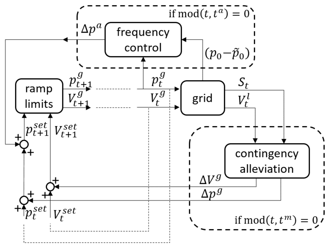
Figure 3 illustrates the control process. For each time step $t$ of the simulation, for given value of $(\mathbf{p}^{g},\mathbf{V}^{g})$, the grid computes the values of the dependent variables $(\mathbf{V}^{l},\mathbf{S})$. Every $t^{m}$ seconds the algorithm determines an optimal step of corrective action to alleviate possible contingencies, as variation of the control variables $(\mathbf{\Delta p}^{g},\mathbf{\Delta V}^{g})$. Similarly, every $t^{a}$ seconds, the frequency control loop computes the imbalance $p_{0}-\widetilde{p}_{0}$ at the slack bus and evaluates $\mathbf{\Delta p}^{a}$ in order to balance it. Then, given the set points $(\mathbf{p}^{set},\mathbf{V}^{set})$, the values of $(\mathbf{p}^{g},\mathbf{V}^{g})$ are computed for each PV-bus for the next time step $t+1$, considering its ramp rate limits.

The proposed method monitors the apparent power flows $S_{ij}$ to detect and quantify line overloads. It could easily be modified to use the line currents $I_{ij}$ for this purpose.

The first goal of the algorithm is to evaluate the presence of violations of voltage or power flow limits. We initially consider the following objective function:

where the parameter $\mu$ controls the weight of the voltage violation term with respect to the line overload one. Parameter $k$ (MVA/pu) is used to convert power flows into per unit. $\mathcal{L}$ is equal to 0 when there are no constraint violations, while it is positive when an operating limit is not respected. However, the objective function should be sensitive to constraints that are “close” to be violated, so that further control actions do not cause additional violations of operating constraints. Accordingly, we introduce the function $g(\tau,\epsilon)$ defined as:

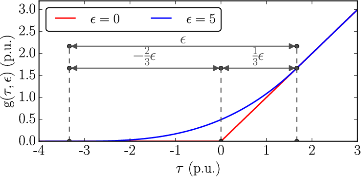
Figure 4 illustrates the shape of this function. The red line shows $g(\tau,\epsilon)$ when $\epsilon=0$, which corresponds to the unpenalized function, i.e., $\mathrm{max}(\tau,0)$, while the blue line illustrates $g(\tau,\epsilon)$ when $\epsilon=5$. Note that $g(\tau,\epsilon)\geq 0$ for $\tau\geq-\nicefrac{{2}}{{3}}\epsilon$. Therefore, the objective function is greater than 0 when a line or a voltage is close to its limit but there is no actual constraint violation.

To simplify the notation we introduce the following functions:

where $\xi\in[0,1]$ controls the shape of $g^{V}$ and $g^{S}$. Using these notations, we introduce the penalized modified function:

The aim of the corrective action algorithm is to iteratively modify the control variables $(\mathbf{p}^{g},\mathbf{V}^{g})$ to alleviate the contingencies. To this effect, we need to determine a quick and reliable path for $(\mathbf{p}^{g},\mathbf{V}^{g})$ that respects their ramp rate limits. Each $t^{m}$ seconds, the algorithm receives the measurement of $(\mathbf{V}^{l},\mathbf{S})$ and computes the value of $(\mathbf{\Delta p}^{g},\mathbf{\Delta V}^{g})$ that minimizes $\mathcal{L^{\prime}}$ while respecting the following ramp rate constraints:

where $R_{g}$ (MW/s) is the ramping limit on $p_{g}$ and $T_{g}$ (p.u./s) is the ramping limit on $V_{g}$. Because voltage regulators are very fast, ramping limits on voltage set-points in (5b) are not a physical constraints like the ramping constraints on active power set-points in (5a). However, we include them because rapid changes in voltage magnitudes are undesirable. If needed, $T_{g}$ can be set to $\infty$ to remove these constraints. At each iteration, we wish to compute the optimal $(\mathbf{\Delta p}^{g},\mathbf{\Delta V}^{g})$ that can be implemented before the following measurement. We index with the superscript $m$ the values measured from the grid. The optimization problem that we solve at each iteration is:

where the function $F(\cdot)$ in constraint (6d) represents the power flow equations. It computes the variation of the dependent variables $(\mathbf{\Delta V}^{l},\mathbf{\Delta S})$, due to $(\mathbf{\Delta p}^{g},\mathbf{\Delta V}^{g})$. Constraint (6e) imposes the active power balance. Otherwise, eventual imbalances would be compensated by the frequency control loop in the form of a distributed response of the generators. Constraints (6f) and (6g) force the active power injection and voltage magnitude at each PV bus to remain within their feasible region. Finally, constraints (6h) and (6i) impose limits on the ramp rates. The optimization problem is non-linear due to constraint (6d).

Changes in active and reactive power injections are related to changes in voltage magnitude and phase by:

where $J$ is the Jacobian matrix. Factoring $J$ is time consuming for large systems. In order to simplify the computation we use the fast decoupled power flow assumptions [30]. We assume that $V_{i}\approx 1$ p.u., $\text{cos}\delta_{i}\approx 1$ and $\text{sin}\delta_{i}\approx 0$, $\forall i\in N^{+}$. Thanks to these assumptions we can decouple the frequency and the voltage control. This leads to:

The simplified Jacobian is now constant over $t$, so it is sufficient to compute it once at the beginning of the simulation. Aiming in substituting (6d) with an alternative linear formulation, we need to evaluate $\frac{\partial\mathbf{S}}{\partial\mathbf{p}^{g}}$, $\frac{\partial\mathbf{S}}{\partial\mathbf{V}^{g}}$ and $\frac{\partial\mathbf{V}^{l}}{\partial\mathbf{V}^{g}}$. For computing $\frac{\partial\mathbf{V}^{l}}{\partial\mathbf{V}^{g}}$, we first evaluate the differential $\text{d}\mathbf{q}^{l}$, where $\mathbf{q}^{l}=\{q_{l},l\in N^{l}\}$. In accordance with (8b), we write:

The term $\text{d}\mathbf{q}^{l}$ is equal to 0 by definition, given that there is no control on the injection of reactive power at a PQ bus. This leads to:

Then, computing $\frac{\partial\mathbf{V}}{\partial\mathbf{V}^{g}}$ is straightforward. Indeed, $\mathbf{V}=\{V_{0},\mathbf{V}^{g},\mathbf{V}^{l}\}$ and

To compute the term $\frac{\partial\mathbf{\delta}}{\partial\mathbf{p}^{g}}$ we invert (8a), i.e.,

Thanks to the fast decoupled power flow assumptions, we obtain:

Finally, we compute $\dfrac{\partial\mathbf{|S|}}{\partial\mathbf{p}^{g}}$ and $\dfrac{\partial\mathbf{|S|}}{\partial\mathbf{V}^{g}}$ as:

The fast decoupled power flow approximation introduced in Section IV-B allows us to replace constraint (6d) with the following set of constraints:

Even though we compute the sensitivities under the decoupled power flow assumptions, the optimization problem (6) can not be decomposed between the control variables $\Delta\mathbf{p}^{g}$ and $\Delta\mathbf{V}^{g}$. Since $|S_{ij}|=\sqrt{P^{2}_{ij}+Q^{2}_{ij}}$, they both influence $\Delta|S_{ij}|$. However, the linearization of $\partial|S_{ij}|$ in equations (15) and (16) may lead to mistakes when $Q_{ij}\ll P_{ij}$ or, less likely, $P_{ij}\ll Q_{ij}$. Therefore, we prefer to impose some artificial upper limits on $P_{ij}$ and $Q_{ij}$, i.e., $\overline{P}_{ij}$ and $\overline{Q}_{ij}$. We evaluate them by imposing the following conditions:

Thanks to condition (18a) we ensure that, if $|P_{ij}|<\overline{P}_{ij}$ and $|Q_{ij}|<\overline{Q}_{ij}$, then $|S_{ij}|<\overline{S}_{ij}$. Then, (18b) imposes that, in case of a violation, the penalty for $|P_{ij}|$ and $|Q_{ij}|$ will be proportional to their contribution to the violation of $\overline{S}_{ij}$. The value of $\overline{P}_{ij}$ and $\overline{Q}_{ij}$ can be computed as

In this way, we can also decompose (6) into two independent subproblems. The first, is solved to evaluate the optimal step $\mathbf{\Delta p}^{g}$ and its objective function is

where $g^{P}_{ij}(\cdot)$ is defined as

We introduce the term $\sum_{g\in N^{g}}|\Delta p_{g}|$ in (21) to force the model to select only the generators that have a significant capacity to alleviate the contingency. The weight of this term in $\mathcal{L}^{p}$ is controlled through the parameter $\nu^{p}$. The optimization problem to evaluate $\mathbf{\Delta p}^{g}$ is:

The second optimization problem determines the optimal step $\mathbf{\Delta V}^{g}$, and its objective function is:

where $g^{Q}_{ij}(\cdot)$ is defined as

As in Eq. (21), we introduce the term $\sum_{g\in N^{g}}|\Delta V_{g}|$ and control its weight in (24) through the parameter $\nu^{v}$. The second optimization problem is:

The non-linearities in (23) and (26) are replaced with alternative linear formulations. In particular, the functions $g^{P}(\cdot)$, $g^{Q}(\cdot)$ and $g^{V}(\cdot)$ are replaced by piece-wise linear approximations. The absolute values are removed through a conventional linearization technique [31]. The result is an LP model, easily solved using a standard optimization engine [32].

Algorithm 2 is used to perform a static simulation of the system’s operation. At each time step $t$, the network solves the power flow equations for given $(\mathbf{p}^{g},\mathbf{V}^{g})$ and evaluates $(\mathbf{V}^{l},\mathbf{S})$. Then, each $t^{m}$ seconds it performs Algorithm 1 to evaluate $\mathbf{\Delta p}^{g}$ and $\mathbf{\Delta V}^{g}$ and modifies the set-point of $(\mathbf{p}^{g},\mathbf{V}^{g})$ accordingly. Similarly, each $t^{a}$ we model the frequency control action by measuring the imbalance at the slack bus and modifying the set-points $(\mathbf{p}^{g},\mathbf{V}^{g})$ in order to compensate for an imbalance. At each time step $t$ we move $(\mathbf{p}^{g},\mathbf{V}^{g})$ towards their set-point $(\mathbf{p}^{set},\mathbf{V}^{set})$, while imposing the ramp rate limits.We simulate the system evolution for $T$ seconds, starting from a contingency.

In a static environment, a mismatch between power injections and extractions results in a frequency deviation from its nominal value, activating an automatic response from the generators participating in the AGC. In this simplified setup, the frequency is assumed constant, and accordingly the level $p_{l}$ of the loads do not change during the simulation. However, we approximate frequency control loop as follows. Each $t^{a}$ seconds, the frequency controller computes the deviation of the active power injection $p_{0}$ at the slack bus from its nominal value $\widetilde{p}_{0}$ and provides an immediate distributed response to restore the frequency:

where $\eta_{g}$ define the relative contribution of generator $g$ to the compensation of the system imbalance. The weight $\eta_{g}$ is assumed to be:

It can easily be shown that $\sum_{g}\Delta p^{\textrm{a}}_{g}+\left(p_{0}-\widetilde{p}_{0}\right)=0$.

In a dynamic simulation, the imbalance $(p_{0}(t)-\widetilde{p}_{0})$ between generation and consumption results in the system’s frequency $f(t)$ (Hz) deviating from its nominal level $\widetilde{f}$ (i.e., 50 Hz), where $\Delta f(t)=f(t)-\widetilde{f}$. The evolution in time of $\Delta f(t)$ is described by:

where $K_{S}$ (Hz/MW) and $T_{S}$ (s) control the system’s dynamic response and $\ell$ is an auxiliary integration variable. The frequency change affects the loads, whose values deviate form their nominal level by $\Delta p^{f}_{l}(t)$, equal to:

where $D^{f}_{l}$ (MW/Hz) is the damping parameter of load $l$. The generators also react to the frequency variation by $\Delta p^{g}_{l}(t)$, which can be approximated by:

where $R^{f}_{g}$ (Hz/MW) is the frequency regulation parameter of generator $g$. Finally, the AGC response $\Delta p^{\textrm{a}}_{g}(t)$ is given by:

where $K^{\textrm{a}}_{g}$ (MW) controls the AGC response of generator $g$.

In the static simulations, three types of contingencies are considered: line overloads, voltage violations, and combinations of line overloads and voltage violations.

Figure 6 compares the evolution of $\mathcal{L}$ and $\mathcal{L^{\prime}}$ over time for an overload of 15 MW on line 67. $\mathcal{L}$ decreases at a constant rate up to around $t=110$ s, after which point it decreases at a slower rate. The explanation for this change can be found on Figs. 7 and 8. Figure 7 shows the changes in active power injections that the algorithm implements to remove this overload. Figure 8 shows how the flows in all the lines change as a result of these corrective actions. The area between the continuous and dashed red lines is the region where the penalized objective function is sensitive to flows that are close to their maximum. At $t\approx$ 110 s, line 118 enters in this penalized region and forces a change in the way the algorithm adjusts the control variables. At $t\approx$ 240 s, $\mathcal{L}=0$ indicating that the overload has been removed. At that time $\mathcal{L^{\prime}}$ is not quite zero because some line flows are close to their limit.

We also tested how the corrective action algorithm performs when inaccurate line susceptances are used to compute the sensitivities, e.g., $\frac{\partial\mathbf{S}}{\partial\mathbf{p}^{g}}$. Let $b_{ij}$ be the actual susceptance of line $(ij)$ and $\widetilde{b}_{ij}$ the value used in the algorithm. $\widetilde{b}_{ij}$ is given by:

where $\beta_{ij}\sim\mathcal{N}\left(\mu_{\beta},\sigma^{2}_{\beta}\right)$ and $\mu_{\beta}=1$, $\sigma_{\beta}=0.2$. This translates in an expected difference between $\widetilde{b}_{ij}$ and $b_{ij}$ of around 16%. Parameter $\beta_{ij}$ is different for each susceptance and is added to all the susceptances simultaneously. We ran 200 simulations for a contingency $C$ of 10 MW on lines 5, 30, 37, 67, 160, and 182. These simulations also consider that some measurements (e.g., $S_{ij}$) may not always be updated in time. To simulate this effect, at each iteration, the power flow in one randomly selected line is not updated. The algorithm uses the previous value for this flow measurement. Table II summarizes the results and shows that the proposed algorithm is still able to remove the violations in 100% of the tests performed.

To create voltage violations we modified the reactive power injection separately at PQ buses 9, 38, 53, 63, 81 and 109. Figure 9 shows how the value of $\mathcal{L}$ evolves in response to the corrective actions deployed for these 6 voltage violations. Figure 10 shows how the algorithm adjusts the voltage set-points at PV buses 59, 65 and 66 to correct a voltage violation at bus 63. Figure 11 compares the values of $\mathcal{L}$ and $\mathcal{L^{\prime}}$ over $t$ for this voltage violation at bus 63. Figure 12 illustrates the evolution of the voltage magnitudes at all PQ buses. Most of the voltages are not affected by the corrective actions because voltage problems are typically local. At the end of the simulation all the voltages are within the acceptable range, including bus 63.

The last set of static simulations considers simultaneous voltage violation and line overload. We ran the simulations considering each combination of the voltage violations and the line overloads of Section VI-A, for C of 5 MVA. Figure 13 illustrates how $\mathcal{L}$ evolves during these 402 simulations, all of which converge in less than one minute. In this figure, the 6 simulations involving an overload of line 67 are highlighted. In all these 6 cases, the rate at which $\mathcal{L}$ decreases at one point during the simulation. This is because voltage violations are corrected more quickly than line overloads because the active power output of generators changes more slowly than their terminal voltage. This change in rate occurs when the voltage violation has been cleared, while line 67 is still overloaded.

In the dynamic simulation, the parameters $K_{S}$ and $T_{S}$ are set at 0.05 Hz/MW and 10 s, respectively. The damping parameter of the loads $D^{f}_{l}$ is:

where $p_{l}(0)$ is the nominal value of the load and $D^{f}$ is 20 MW/Hz. $R^{f}_{g}$ and $K^{\textrm{a}}_{g}$ are given by:

where $R^{f}$ and $K^{\textrm{a}}$ are 0.005 Hz/Mw and 80 MW, respectively.

We use the dynamic simulation to analyze the consequences of the outage of line 30 at $t=20$ s, which causes overloads on lines 31, 35, 37, 42, and 180. In this case the algorithm needs to recompute the sensitivity matrices because the topology of the grid has changed. Calculating these sensitivities requires a one-time computation of about 80 ms, while the LP problems (23) and (26) are solved in around 20 ms (each $t^{m}$ seconds). Figure 14 shows how the value of $\mathcal{L}$ evolves as the corrective actions are implemented by the proposed method. $\mathcal{L}$ is 0 up to 20 s, as no violation has yet arisen. After the failure of line 30, $\mathcal{L}$ increases to almost 8000 p.u. and is then brought back to 0 (i.e., no overloads) in around 180 s. Figure 15 illustrates the normalized flows in the transmission lines during this dynamic simulation, highlighting the 5 lines that overloaded after the failure of line 30. In particular, line 31 is severely overloaded (almost 80% above its maximum limit) and is the last one to be returned to an acceptable value. Figure 16 shows how the system’s frequency $f$ evolves during the simulation. Note the small drop in frequency at $t=20$ s (i.e., when line 30 fails), which is rapidly restored by the AGC. After this event, the frequency is stable and barely affected by the corrective actions because the proposed algorithm coordinates the adjustments in the power outputs of the generator buses in a way that ensures that the total power injection is constant (see constraint (23e) in model (23)).

References

- [1] P. Panciatici, M. Campi, S. Garatti, S. Low, D. Molzahn, A. Sun, and L. Wehenkel, “Advanced optimization methods for power systems,” in Power Systems Computation Conference (PSCC), 2014. IEEE, 2014, pp. 1–18.
- [2] L. Roald, S. Misra, T. Krause, and G. Andersson, “Corrective control to handle forecast uncertainty: a chance constrained optimal power flow,” IEEE Trans. Power Syst., vol. 32, no. 2, pp. 1626–1637, 2017.
- [3] A. Monticelli, M. Pereira, and S. Granville, “Security-constrained optimal power flow with post-contingency corrective rescheduling,” IEEE Trans. Power Syst., vol. 2, no. 1, pp. 175–180, 1987.
- [4] R. Bacher and H. P. Van Meeteren, “Real-time optimal power flow in automatic generation control,” IEEE Trans. Power Syst., vol. 3, no. 4, pp. 1518–1529, 1988.
- [5] L. Gan and S. H. Low, “An online gradient algorithm for optimal power flow on radial networks,” IEEE J. Sel. Areas Commun., vol. 34, no. 3, pp. 625–638, 2016.
- [6] N. Balu, T. Bertram, A. Bose, V. Brandwajn, G. Cauley, D. Curtice, A. Fouad, L. Fink, M. G. Lauby, B. F. Wollenberg et al., “On-line power system security analysis,” Proceedings of the IEEE, vol. 80, no. 2, pp. 262–282, 1992.
- [7] F. Capitanescu, M. Glavic, D. Ernst, and L. Wehenkel, “Contingency filtering techniques for preventive security-constrained optimal power flow,” IEEE Trans. Power Syst., vol. 22, no. 4, pp. 1690–1697, 2007.
- [8] F. Capitanescu, T. Van Cutsem, and L. Wehenkel, “Coupling optimization and dynamic simulation for preventive-corrective control of voltage instability,” IEEE Trans. Power Syst., vol. 24, no. 2, pp. 796–805, 2009.
- [9] S. Chatzivasileiadis and G. Andersson, “Security constrained opf incorporating corrective control of hvdc,” in Power Systems Computation Conference (PSCC), 2014. IEEE, 2014, pp. 1–8.
- [10] D. Phan and J. Kalagnanam, “Some efficient optimization methods for solving the security-constrained optimal power flow problem,” IEEE Transactions on Power Systems, vol. 29, no. 2, pp. 863–872, 2014.
- [11] Y. Liu, M. C. Ferris, and F. Zhao, “Computational study of security constrained economic dispatch with multi-stage rescheduling,” IEEE Transactions on Power Systems, vol. 30, no. 2, pp. 920–929, 2015.
- [12] T. Medicherla, R. Billinton, and M. Sachdev, “Generation rescheduling and load shedding to alleviate line overloads-system studies,” IEEE Trans. Power App. Syst., no. 1, pp. 36–42, 1981.
- [13] A. Shandilya, H. Gupta, and J. Sharma, “Method for generation rescheduling and load shedding to alleviate line overloads using local optimisation,” in IEE Proceedings C-Generation, Transmission and Distribution, vol. 140, no. 5. IET, 1993, pp. 337–342.
- [14] P. Bijwe, D. Kothari, and L. Arya, “Alleviation of line overloads and voltage violations by corrective rescheduling,” in IEE Proceedings C (Generation, Transmission and Distribution), vol. 140, no. 4. IET, 1993, pp. 249–255.
- [15] M. E. Arini, “Fast method to alleviate line overloads by corrective generation rescheduling and load shedding,” Electric machines and power systems, vol. 25, no. 4, pp. 355–370, 1997.
- [16] D. Hazarika and A. Sinha, “Method for optimal load shedding in case of generation deficiency in a power system,” International Journal of Electrical Power & Energy Systems, vol. 20, no. 6, pp. 411–420, 1998.
- [17] B. Talukdar, A. Sinha, S. Mukhopadhyay, and A. Bose, “A computationally simple method for cost-efficient generation rescheduling and load shedding for congestion management,” International Journal of Electrical Power & Energy Systems, vol. 27, no. 5, pp. 379–388, 2005.
- [18] A. Y. Abbas, S. E. G. M. Hassan, and Y. H. Abdelrahim, “Transmission lines overload alleviation by generation rescheduling and load shedding,” Journal of Infrastructure Systems, vol. 22, no. 4, p. A4016001, 2016.
- [19] B. Otomega, A. Marinakis, M. Glavic, and T. Van Cutsem, “Model predictive control to alleviate thermal overloads,” IEEE Transactions on Power Systems, vol. 22, no. 3, pp. 1384–1385, 2007.
- [20] M. R. Almassalkhi and I. A. Hiskens, “Model-predictive cascade mitigation in electric power systems with storage and renewables—part i: Theory and implementation,” IEEE Transactions on Power Systems, vol. 30, no. 1, pp. 67–77, 2015.
- [21] L. Lenoir, I. Kamwa, and L.-A. Dessaint, “Overload alleviation with preventive-corrective static security using fuzzy logic,” IEEE Trans. Power Syst., vol. 24, no. 1, pp. 134–145, 2009.
- [22] K. Pandiarajan and C. Babulal, “Overload alleviation in electric power system using fuzzy logic,” in Computer, Communication and Electrical Technology (ICCCET), 2011 International Conference on. IEEE, 2011, pp. 417–423.
- [23] E. Dall’Anese, A. Simonetto, and S. Dhople, “Design of distributed controllers seeking optimal power flow solutions under communication constraints,” in Decision and Control (CDC), 2016 IEEE 55th Conference on. IEEE, 2016, pp. 7489–7495.
- [24] E. Dall’Anese, K. Baker, and T. Summers, “Optimal power flow for distribution systems under uncertain forecasts,” in Decision and Control (CDC), 2016 IEEE 55th Conference on. IEEE, 2016, pp. 7502–7507.
- [25] X. Zhou, E. Dall’Anese, and L. Chen, “Online stochastic control of discrete loads in distribution grids,” arXiv preprint arXiv:1711.09953, 2017.
- [26] N. Jaleeli, L. S. VanSlyck, D. N. Ewart, L. H. Fink, and A. G. Hoffmann, “Understanding automatic generation control,” IEEE Trans. Power Syst., vol. 7, no. 3, pp. 1106–1122, Aug 1992.
- [27] J. Carpentier, “‘to be or not to be modern’that is the question for automatic generation control (point of view of a utility engineer),” International Journal of Electrical Power & Energy Systems, vol. 7, no. 2, pp. 81–91, 1985.
- [28] N. Chiang and A. Grothey, “Solving security constrained optimal power flow problems by a structure exploiting interior point method,” Optimization and Engineering, vol. 16, no. 1, pp. 49–71, 2015.
- [29] S. Chakrabarti, M. Kraning, E. Chu, R. Baldick, and S. Boyd, “Security constrained optimal power flow via proximal message passing,” in Power Systems Conference (PSC), 2014 Clemson University. IEEE, 2014, pp. 1–8.
- [30] B. Stott and O. Alsac, “Fast decoupled load flow,” IEEE Trans. Power App. Syst., no. 3, pp. 859–869, 1974.
- [31] S. Boyd and L. Vandenberghe, Convex optimization. Cambridge university press, 2004.
- [32] Gurobi Optimization, “Gurobi optimizer reference manual,” 2016. [Online]. Available: http://www.gurobi.com