Rosetta photoelectron emission and solar ultraviolet flux at comet 67P
Abstract
The Langmuir Probe instrument on Rosetta monitored the photoelectron emission current of the probes during the Rosetta mission at comet 67P/Churyumov-Gerasimenko, in essence acting as a photodiode monitoring the solar ultraviolet radiation at wavelengths below 250 nm. We have used three methods of extracting the photoelectron saturation current from the Langmuir probe measurements. The resulting dataset can be used as an index of the solar far and extreme ultraviolet at the Rosetta spacecraft position, including flares, in wavelengths that are important for photoionisation of the cometary neutral gas. Comparing the photoemission current to data measurements by MAVEN/EUVM and TIMED/SEE, we find good correlation when 67P was at large heliocentric distances early and late in the mission, but up to 50 percent decrease of the expected photoelectron current at perihelion. We discuss possible reasons for the photoemission decrease, including scattering and absorption by nanograins created by disintegration of cometary dust far away from the nucleus.
Keywords:
comets: individual (67P/Churyumov-Gerasimenko) – Sun: UV radiation – methods: data analysis – plasmas – dust, extinction1 Introduction
ESA’s comet-chaser Rosetta arrived at comet 67P/Churyumov-Gerasimenko in August 2014 and completed its mission in September 2016. During all this time, the instruments of the Rosetta Plasma Consortium (RPC) were monitoring the plasma environment. The Langmuir probe instrument (RPC-LAP), described in detail by Eriksson et al. (2007), measures the current between the probe and surrounding space with the aim to characterise the plasma. When the probes are sunlit, they also measure the current due to excitation and emission of electrons from light, as discovered by Hertz (1887) and famously interpreted by Einstein (1905). The photoemission saturation current of a Langmuir probe depends on the solar far and extreme ultraviolet spectrum, and has successfully been used as a proxy for the solar UV flux on previous studies around Venus (Brace et al., 1988; Hoegy et al., 1993). For plasma science, the UV flux has implications on spacecraft charging, as well as a fundamental source for plasma from the ionisation of neutrals around e.g. a comet (Vigren et al., 2016; Vigren & Galand, 2013; Bodewits et al., 2016; Galand et al., 2016). The photoemission, like the solar flux, should follow a relation as Rosetta approaches and retreats from comet perihelion.
We compare the photoemission observed by RPC-LAP from May 2014 to the end of mission in September 2016 to the expected photoemission using UV observations from the SEE experiment (Woods et al., 2005) on the TIMED spacecraft orbiting Earth and the EUVM experiment (Eparvier et al., 2015) on the Maven mission at Mars. The orbits of Mars and 67P were such that MAVEN and Rosetta were on the same side of the Sun during most of the Rosetta mission, although there are times when Rosetta is better aligned with the TIMED/SEE at Earth, with the added benefit of superior wavelength resolution.
We use three independent techniques for estimating the maximum photoemission current of a negatively charged probe, the photosaturation current (), one of these techniques is to our knowledge new.
In Section 2, we go through the relevant theory of Langmuir Probes and the photoelectric effect, followed by a description of each technique to obtain the photoemission current from the probes as well as the estimates from UV observations. In Section 3 we present our results, discuss their implications in regards to attenuation of gas and dust or contamination in Section 4, followed by conclusions in Section 5.
2 Methods
Conductive objects such as the Langmuir probes on Rosetta will emit electrons when subjected to sunlight due to the photoelectric effect. For cases when none of the electrons are reabsorbed by the probe, such as a negatively charged probe, the photosaturation current can be observed. The theory behind Langmuir Probe measurements is described in Section 2.1, and three different techniques to observe is described in Section 2.2, 2.3 and 2.4. We also propagate the UV observations around Earth and Mars to the Rosetta position, as described in Section 2.5.
2.1 Langmuir probe photoemission and probe theory
A fundamental mode of operation of a Langmuir probe is the bias voltage sweep. During a sweep, the probe is measuring the current to the probe while stepping through a series of bias voltages set with respect to the spacecraft ground. The absolute potential between the probe and a plasma at infinity is thus , where is the spacecraft potential. The current to the probe can be separated into three parts: ion (), electron () and secondary electron emission current. The secondary emission current can be subsequently separated into photoemission () and secondary electron emission from particle impact (). Akin to the photoemission current, will depend on material properties of the probe but is also directly proportional to the ion and electron current to the probe such that if , , and can in most cases be assumed to be negligible.
It can be shown (Medicus, 1961; Mott-Smith & Langmuir, 1926) that the electron current to a spherical probe is given by
| (1) |
where is the random current for electrons, given by
| (2) |
where is the plasma density, is the electron temperature and is the surface area of the Langmuir probe and other constants have their usual meaning.
For supersonic ion flow of single positive charge, the ion current to a sphere is shown by Fahleson et al. (1974) to be
| (3) |
where is the energy of ions of mass and flow speed , is the ram current, given by
| (4) |
where is the circular cross section of the probe.
For a negatively charged probe, the photoemission current is then at its saturation value which depends on the UV sun flux at each wavelength , the surface area normal to the sunlight , as well as the photoelectron yield of the probe material, defined as number of emitted electrons per incident photon. Following Grard (1973), and defining to be in units of photons s-1m-2, we obtain:
| (5) |
In absence of photoelectron yield measurements for TiN, we follow the approach inspired by Brace et al. (1988) and Hoegy et al. (1993) in a similar situation. They used a yield function adapted from an average of metals examined by Feuerbacher & Fitton (1972); Canfield & Swanson (1987) with a free numerical factor to scale the estimated photosaturation current from Equation 5 to the measured photoemission, using sun flux measurements of other spacecraft. In our case the free numerical factor turned out to be very close to 1 between the MAVEN/EUVM UV spectra and our photoelectron yield. We therefore adopted the yield function plotted in Figure 1 with no further tuning or correction.
TIMED/SEE spectral irradiance data includes uncorrected degradation beginning in late 2011, resulting in irradiances that become increasingly lower with time than those measured by other spacecraft (SDO/EVE). Therefore the free numerical factor differed from 1 when we used TIMED/SEE data.

2.2 Probe photoemission current from Sun-shadow transitions
The component of the total probe current due to photoemission from the probe surface, , clearly vanishes for a probe that is not sunlit. Therefore, an obvious way of measuring the photoemission current of a probe is by comparing the probe current at fixed voltage-bias just before and after it goes into or out of shadow. This seemingly straightforward method requires at least two conditions to be met: (1) the probe must be at a negative potential w.r.t. the local plasma at the position of the probe in order for the full photosaturation current to be sampled, limiting the dataset to probe sun/shade transitions during which LAP1 is commanded at a negative bias potential w.r.t. the spacecraft; (2) concurrent variations in probe current due to other factors, e.g. varying plasma density, temperature, drift velocity etc., must be either negligible in comparison to the photoemission current, or occur on sufficiently short time-scales that their effects can be filtered out. In practice, this limits the applicability of the method to probe sun/shade transitions that are sufficiently fast for the general background ion current to be essentially a stationary process, but at the same time separated by sufficient time for calculation of statistical moments of this process, e.g. arithmetic mean and standard deviation. We have in this study decided to use only probe sun/shade transitions in which the probe goes from completely sunlit to completely shaded, or vice versa, in no more than two minutes, preceded and succeeded by periods of complete sunlight or shade for at least two minutes.
Figure 2 (left) shows a sketch of the Rosetta spacecraft and RPC-LAP. The solar panels were almost always held orthogonal to the Sun, meaning the S/C Y-axis stayed perpendicular to the sun. When the spacecraft turned around its Y-axis, which happened regularly, LAP1 would become completely shadowed by the spacecraft solar array. In Figure 2 (right) we define the Solar Aspect Angle (SAA), as the angle between the spacecraft +Z and the direction of the Sun, counted positive when the Sun moved from +Z toward +X.

Figure 3 shows an example from March 3, 2015, where LAP1 goes from shadow to sunlight. The actual sun/shade transition, during which the probe is partially sunlit and hence draws a successively increasing photoemission current, is marked by the grey patch in the figure. The solar aspect angles at which the probe enters and exits partial illumination conditions are shown in the figure; they are and , respectively. For LAP1 there is also a second possible transition region between and which is also used in this study, when available. For visual reference, see Figure 2.

The magnitude of the current jump across the transition region is calculated by taking the difference of the arithmetic means of the probe current during the 2-minute periods immediately preceding and succeeding it, shown as blue and red lines, respectively, in Figure 3. As can be seen in Figure 3, the probe current is prone to brief pulses of considerably increased magnitude. These have been interpreted as cold plasma filaments passing by the spacecraft (Eriksson et al., 2017) and produce a substantially skewed distribution about the mean of the sample currents. Therefore, following Tukey (1977), all sample currents that lie more than 1.5 times the interquartile range below the first quantile or above the third quantile are discarded as outliers.
Sample standard deviations and are computed taking into account sample auto-correlation using the method of Zieba (2010) (specifically their Equation (10)). Corresponding confidence intervals at the 95% level, , with the number of samples, are shown in Figure 3 as blue and red shaded regions, respectively. A confidence interval for the difference of the means is then simply obtained as .
This method for measuring the probe photoemission current has the advantage of being unaffected by any potential additive offsets in the current measurements, since it relies on a current difference and not the absolute value. Its main shortcoming is that its application is contingent on specific attitude and commanding criteria, as previously mentioned, and as thus a rather sparse and uneven dataset. During the entire autumn of 2014, there is not a single sun/shade transition of LAP1 coinciding with commanded negative fixed bias voltage. This situation was somewhat remedied by the fact that the ion current in the frequent sweeps during this time of low cometary activity far away from the Sun was entirely negligible compared to the photoemission current. Therefore, photoemission estimates from August to October 2014 was obtained from the difference of the currents at large negative bias voltages between sweeps immediately before and after a sun/shade transition. Specifically, we obtain arithmetic means and standard deviations from the currents at the lowest 5 V of bias potentials in each sweep, allowing us to estimate confidence intervals of the photoemission current for each transition.
2.3 Probe photoemission from single sweeps
Throughout the Rosetta mission, the Langmuir probe instrument has seen a very dynamic and varying plasma with regions where ion, electron and photoemission current have, within the bias voltage range of the Rosetta Langmuir probe, each individually dominated the Langmuir probe sweep measurement (Eriksson et al., 2017). For sunlit probes, an automatic routine was set to find the knee in the I-V curve, as previously described by Odelstad et al. (2016), and by proxy, , to subdivide the I-V curve into two regions of . Assuming the spacecraft potential is well within the voltage bias sweep of V, the two regions will be characterized by the linear ion current and the photosaturation current for and a linear electron current for . Using the fact that at from Equations 1 and 3, we use an automatic fitting routine to remove a model of the electron and ion current component to obtain only the current contribution from and . The latter can be assumed to be negligible for all but the densest of plasmas, such that for negative we can obtain . An example of the sweep current fitting routine result is shown in Figure 4.

The accumulated errors from a single estimate with this technique is expected to be large, owing to the many mutually dependent fits needed to procure the estimate, as well as the noise level of the instrument. Indeed, there are times were the automatic routine does not produce physically meaningful results, and as such only 92% of the dataset was used due to inexactness of the automatic routine, interference or erroneous commanding. The automatic routine and the threshold of validity used are still in development, so to limit the impact of erroneous estimates, we present the median result over an operational block, defined as a period when the instrument is operated in one single operational mode (on average 400 measurements over 3-4 hours), and the Median Absolute Deviation (MAD) in Figure 6.
The largest source of random error is estimated to arise in the electron model fit, in a region where we often see a non-well-behaving current, as well as the difficulties of correctly estimating , as studied in greater detail by Odelstad et al. (2016). However, as the sample size is very large (around 400,000) we expect to become much less sensitive to random errors as we take a median of the results. Of all uncertainties involved, the dominant source is expected to be the possible systematic error from secondary emission current. which may give exaggerated values of . If there is a discrepancy between this result and other estimates, we may be able to estimate the impact of secondary electron emission from particle impact on the Langmuir Probes.
2.4 Probe photoemission from analysis of multiple sweeps
Assuming that the photoemission from the probe does not change significantly between sweeps, it is possible to find the photoemission current by combining results from several sweeps. For this purpose, data from the ion saturation region is required, so that the electron current can be taken as negligible. Taking , the total current, assuming no secondary emission by particle impact, detailed in section 2.1 simply reduces to
| (6) |
and the derivative is then
This result combined with Equations 3 and 6 yields
| (7) |
where is given by
Assuming that does not change during the sweeps, we can extrapolate for from a number of measurement of and with enough spread in , as
| (8) |
Although we have so far ignored , we note that for electron emission from ion impact, if it increases linearly with density and for it would be indistinguishable from the ion current and would not affect Equation 8. For other values of it would introduce a small non-linear current slope as the energy of primary collision species increases. Also, as the primary electron current in the specified region is assumed to be negligble, so would its secondary current be. When this is not the case, the secondary current would instead slightly mitigate the effect the primary electron current would have on the photoemission estimate.

Restricted by the condition that needs to be approximately constant during the series of sweeps, it is worth investigating under which range of plasma parameters this method is effective. Note that in order to use Equation 7 to extrapolate we need several data points from sweeps during changing plasma conditions, as illustrated in Figure 5. Although this method is sensitive to both and , the plasma environment around Rosetta varies much faster in density, with order of magnitude density fluctuation time-scales of minutes to seconds as reported by Henri et al. (2016) as well as the diurnal variation evident by the data in Odelstad et al. (2015). In comparison, the ion velocity appears much more stable (Vigren et al 2017, this issue), but will still introduce some random error. We investigate this theoretically in Appendix A. In Section 3 we will find that all three methods agree well, suggesting small errors in practise.
The dataset from the multiple sweep method and the variance of the fit is plotted in Figure 6, Results with large variances in the linear ion slope, and as such, large non-linear effects from e.g. the electron retardation current, are discarded.
2.5 Propagation of TIMED/SEE and MAVEN/EUVM data to Rosetta
Rosetta does not carry any instrument for direct measurement of solar UV flux at the position of the spacecraft. For comparison, we rely on measurements from TIMED/SEE at Earth and MAVEN/EUVM at Mars, propagated out to the position of 67P. The propagation procedure consists of finding the last preceding and first succeeding epochs at which the ’source’, Earth or Mars, respectively, was at the same solar longitude as that of Rosetta at the queried epoch. The measured UV flux at these epochs are then scaled by the square of the respective heliocentric distances of the source divided by that of Rosetta at the queried epoch. Finally, a weighted average of the two scaled EUV measurements at the source is computed such that the value of the closest measurement taken less than a few days before or after the queried epoch was used, otherwise the two values are weighted together by a linear interpolation of their respective temporal separation from the queried epoch.
The datasets used for the propagation are Level 3 daily averages from the TIMED/SEE database (Woods et al., 2005) and Level 3 daily averaged spectral irradiance (non-flare background data) from MAVEN/EUVM (Thiemann et al., 2017a) and the propogated results are plotted in Figure 6. The shaded regions in Figure 6a corresponds to periods where Mars (purple) and Earth (green) was within a 45∘ azimuth sector of Rosetta in the elliptical plane, where we expect optimal correlation. It should be noted that Mars never was further than 72∘ behind Rosetta until July 2016.
3 Observations

All three methods to obtain the photo-saturation current correlate well with each other both on the global scale and the small scales in Fig 6a, resolving the solar sidereal rotation period of 24.5 days. In particular, the good agreement between the three different methods verifies the methods and suggests that the we are not heavily influenced by the many individually unique error sources for each method.
The two EUV photoemission estimates derived from MAVEN/EUVM and TIMED/SEE data agree over the entire period with negligible differences between them if we scale the TIMED/SEE data by a factor of 1.2, in an attempt to correct for the known degradation on TIMED/SEE since late 2011. The scaling could also be analogous of a slightly larger photoelectron yield, and is still very reasonable from the photoelectron yield dataset (Feuerbacher & Fitton, 1972).
The photosaturation current obtained from single sweeps cannot distinguish between secondary emission from photon or particle impact, and around perihelion (Aug 2015), where we expect high densities and collisions to be more frequent, we obtain a much higher estimate than the other methods at certain points. As evident by the large variance of these points in the single sweep method in Figure 6b, the uncertainties at perihelion are large, and as such, these points of the single sweep method data should be ignored. However, subtracting the single sweep estimates from the multiple sweep estimates, we could obtain estimates of the secondary emission from particle impact from the probe (although not done in this report). This is otherwise impossible to observe directly with LAP. We can also use this to estimate when we safely can assume impact emission to be negligible.
Also evident in the result and variance of the data are brief large-amplitude changes of photoemission, which upon inspection correlate with solar flares (e.g. X1.6 flare 2014-10-22, M4.5 flare 2015-11-20).
The mission typical 30-160 s cadence of the Langmuir Probe sweep is in theory more than enough for detecting most flares in EUV (Aschwanden et al., 2014; Thiemann et al., 2017b). However individual probe sweeps may have significant noise, due to the plasma conditions and other error sources, complicating such detection. More than anything the processing (binning, averaging) of the dataset in this report limits the detection to Long Decay Events (LDEs) with durations on the order of hours, typically reserved for the largest GOES X-ray flare classes (X and M) (Aschwanden & Freeland, 2012). In a study by Aschwanden et al. (2014), they conclude that their channel of largest wavelength, 30.4 nm is the optimal for detecting flares in the EUV. As seen in Figure 1, the RPC-LAP probes can be expected to have good sensitivity to these wavelengths.
4 Discussion
As can be seen in Figure 6c, the UV flux derived from probe photoemission is about as expected at the start and end of the mission, but smoothly drops to about half its expected value around perihelion. There seems to be some shortfall also at end of mission, but data variability here is much more pronounced. Nevertheless, it is clear that the photoemission has a drop around perihelion, from which it at least partially recovers as Rosetta follows the comet outward.
We will discuss possible explanations of this photoemission decrease including contamination in Section 4.1 and attenuation by comet gas or dust in Section 4.2 and 4.3, but we note first that: (1) the orbital inclination of Comet 67P of from the planetary ecliptic plane, would give us a slightly different Sun flux than measured by MAVEN/EUVM or TIMED/SEE, but the effect would be limited and much less than observed; (2) the good agreement for all three methods suggests that we are not significantly affected by offsets and unique individual error sources; (3) the uncertainty in the photoelectric yield of TiN may affect the estimated on small scales, but even a vastly different yield profile would not change the deviation around perihelion since there is no significant trend in any wavelength channel that influences the result other than the dependence over the course of the mission.
4.1 Contamination
Effects on the probe surface such as contamination, which could introduce a resistance and a net reduction in emitted current, would either be expected to be cumulative over the entire mission or be less during periods when the comet-spacecraft distance is large such as the day-side (Sep-Oct 2015) or night-side excursion (Mar-Apr 2016). In addition, a contamination in form of a resistive and capacitive layer should be discernible when alternating bias stepping direction (hysteresis sweeps) according to Szuszczewicz & Holmes (1975):
where is the time between two subsequent current measurements on a probe with a capacitance C.
To monitor contamination on the Langmuir probes, more than 23 000 hysteresis sweeps were performed throughout the mission. A summary for LAP1 is plotted in Figure 7, subdivided into two datasets with different starting potentials and time periods. The sweeps are either from -30 V up to + 30 V and back down to -30 V (’up-down’) or vice versa (’down-up’).
As evident by the large variance (up to 400 nA, off scale) for the first set of sweeps, the electron current to the probe changes rapidly in comparison to the sweep duration ( s), such that the method was changed during 2016 to an up-down type of sweeps, with clearer results. We find no significant capacitive current contribution, but estimate that at most it would offset our results in the two sweep analysis methods with nA, and is as such negligible. The sun-shadow transition data are unaffected by this capacitive current offset.
On LAP2, we do find evidence of significant contamination, particularly during a few months after the day-time excursion in Oct 2015 with a capacitive current contribution exceeding 20 nA, as well as a significant decrease in photoemission current. The LAP2 results are therefore excluded from this report.

4.2 Attenuation by comet gas
As observed by the Rosetta Alice instrument (Keeney et al., 2017), the neutral gas and dust of the comet coma can absorb a large ( percent) fraction of some spectral lines in the 70-200 nm range of Alice observation. In particular, the common comet gas species of interest with substantial absorption cross-sections within our yield profile would be , and CO. However, Alice absorption observations are along a path close to the comet core, with regions of peak densities, whereas the Probe-Sun path are almost always along more tenuous atmosphere profile due to the terminator plane or dayside orbit of Rosetta, and as such very sensitive to the Rosetta-comet distance , which was above 200 km for several months around perihelion. We have applied the method of Vigren & Galand (2013) to estimate a maximum EUV absorption of only percent by molecules near perihelion at km (the attenuation was calculated along the Sun-Rosetta line assuming a spherically symmetric coma decaying in number density as ). In the same scenario but close to the comet surface the maximum EUV absorption is instead percent at certain wavelengths, and as such not in disagreement with Alice results. Unfortunately there are no direct measurements of incident solar UV from Alice or other Rosetta instruments, and we lack an absolute measure of the incident solar UV at Rosetta to compare with the RPCLAP photoemission.
4.3 Attenuation by cometary dust
Another possible source of EUV extinction would be scattering and absorption of cometary dust grains. Studies on interstellar dust by Cruise (1993) and Kolokolova et al. (2004) indicate that EUV scattering by micrograins and nanograins can be significant. Even so, the large dust grains mainly observed by the GIADA, COSIMA and MIDAS dust instruments (Rotundi et al., 2015; Fulle et al., 2015; Bentley et al., 2016; Hilchenbach et al., 2016) could not, for the amounts reported, provide sufficient surface area for our inferred UV decrease of 50 percent at perihelion. However, the particles investigated with the MIDAS instrument all show agglomerate character with subunit sizes down to the nanometer scale. It is therefore conceivable that cometary dust particles could undergo a process like fragmentation or erosion that leads to the release of their constituent (nano)grains, thus increasing the total surface area and more significant attenuation in UV may result.
If the nanograin production would be most efficient farther away than Rosetta’s position from the comet nucleus, this would explain the absence of a large UV extinction difference for different Rosetta-comet distances (that were, e.g., between 200 and 1000 km in Oct 2015). It is notable that the first direct detections of nanograins at a comet were made during the fly-by at 1P/Halley, which covered distances that were mainly larger than the general Rosetta-comet distance, and that there are measurements suggesting high densities of nanograins at immense (in the order of 106 km) comet distances (Utterback & Kissel, 1990).
From Rosetta at 67P, nanograins were occasionally detected by the Ion and Electron Spectrometer IES (Burch et al., 2015) and seen to flow mainly in the antisunward direction. In addition, the GIADA dust detector noted a three times higher flux of submicron dust particles in the antisolar direction than the flux coming directly from the nucleus (Della Corte et al., 2015). Gombosi et al. (2015) modelled the influence of radiation pressure on grain motion, suggesting nanograins originate from larger grains emitted by the comet and fragmenting at distances of several (tens of?) thousand km sunward of the nucleus. The radiation pressure drives them back toward the comet as seen by IES and GIADA, also yielding a significant nanograin column density in the sunward direction from Rosetta as suggested in our scenario.
In the following we will test if our hypothesis of nanograins absorbing the EUV coming from the Sun can hold. We will check if fragmentation or erosion of a minor amount of dust particles at large distance from the nucleus can lead to a sufficient population of nanograins and estimate the necessary size to account for our observations. We will revisit Rosetta results to ensure their compatibility, and finally discuss the implications of a hypothetical existence of a nanograin population in a certain distance of the comet.
Consider large () grains being produced at the comet surface, ejected isotropically at some velocity , and fragmenting or eroding into smaller particles of radius outside some distance , scattering 100% of their spherical geometric cross section such that the fraction of scattered light is
| (9) |
where is the column density of spherical dust grains small enough for significant UV absorption. This assumes the fraction of scattered light, or the optical depth, to be small and for a more general case we note that Equation 9 becomes:
| (10) |
If we let a fraction of the total mass of the dust cloud undergo fragmentation or erosion, then the total mass per area of dust in a column between Rosetta and the Sun becomes :
where is mass of a dust grain fragmentation product of density . Inserting Equation 9 gives
| (11) |
In a column from to the Sun, where we assume the dust grains have fragmented into small enough particles for significant UV scattering to take place, the mass per area is then
| (12) |
assuming an isotropic density distribution decreasing with from the comet surface at , where the volume average mass density of dust .
Assuming a constant dust-to-gas mass ratio , we can use the production rate of water gas from Hansen et al. (2016), to estimate :
| (13) |
At perihelion for a dust grain with average outflow velocity m/s as reported by Fulle et al. (2015), dust bulk density kgm-3 (Rotundi et al., 2015), dust-to-gas mass ratio (Snodgrass et al., 2016), s-1 (Hansen et al., 2016), and letting of the dust mass fragment and absorb of incoming EUV in a column from = 1000 km to the Sun, we estimate the dust grain radius to be 19 nm.
A spherical dust grain with radius of 19 nm would according to Skolnik (1981) scatter 100 percent of its geometric cross-section of light in wavelength of 119 nm and below, and is as such on the correct length scale for attenuation in RPC-LAP wavelengths. The above considerations are of course very rough, resting on a series of assumptions. Nevertheless they show that the above hypothesis cannot be ruled out directly. An obvious simplification in the model is the singular size of the disintegration product. A size distribution, although useful, should be cemented in a firm understanding of the disintegration process involved, including disintegration products and forces, which we do not pretend to have. However, if the simple model works for a singular size of grains, then it will also work for some distribution of grains. Furthermore, due to our lack of physical model for the disintegration, is more or less a free parameter. However, we chose a value consistent with (1) a negligible decrease of attenuation even during the day-side excursion (Sep-Oct 2015, up to 1000 km sunward), (2) remote observations (Boehnhardt et al., 2016) of 67P dust, discussed in more detail below, and (3) still much less than the apex distance for dust grains as investigated by Gombosi et al. (2015).
To compare these results with other Rosetta observations it should be noted that the presented RPC-LAP measurements were taken by remotely sampling the Rosetta-Sun environment. Rosetta carried a variety of other remote instruments, although most investigated the vicinity of the comet nucleus and rarely sampled sunward. Additionally, the different spectral ranges of the instruments further impede a detection of UV-extinction as, e.g., the scientific camera system on-board OSIRIS is sensitive in the range of 250 - 1000 nm (Keller et al., 2007)), for which the geometric scattering efficiency of 19 nm sized nanograins would decrease to 4 - 0.1% (Skolnik, 1981) and thus possibly escape detection.
As stated in the beginning of this section, the amounts reported in direct observations of large dust grains cannot directly account for the inferred UV attenuation. Our model thus relies on a mechanism of fragmentation or erosion of large grains at larger distances than the typical Rosetta-comet distance. One such mechanism would be erosion and/or evaporation of gluing material (Boehnhardt et al., 2016; Lasue et al., 2007). As this process would be most effective for periods with high solar radiation it would readily account for the strong UV absorption during perihelion whilst fading to absence for increasing comet-Sun distances. This scenario is also in agreement with remote observations of comet 67P from Earth by Boehnhardt et al. (2016), where their observational data suggests dust fragmentation at large comet distances, in particular for perihelion when the vicinity of the comet to the Sun facilitates dust heating and thus material degradation. Furthermore, the modelling work of Gombosi et al. (2015) shows that dust particles ejected sunward may be deflected by solar radiation at a comet distance of some thousand kilometres, and suggest particle fragmentation close to their turn-around point. Finally, as comets are speculated to be a source of nanodust in our Solar System (Mann, 2017), the herein presented hypothesis might aid the understanding of the comet contribution to the Solar System dust.
5 Conclusions
We have presented estimates of the Langmuir Probe photoemission current using three different methods of which one is, to our knowledge, new. All three methods agree very well on global and small scales and enables the use of the Langmuir Probe as an ultraviolet photo-diode on Rosetta. The three methods are further validated by the use of theoretical estimates of the Langmuir probe photoelectron emission using EUV measurements from two other spacecraft, and a suitable estimate for the photoelectron yield of the titanium probe, which agrees very well on the start and end of the mission as well as small scale fluctuation in solar sidereal rotation frequencies. The results in this paper can be used to estimate the solar EUV intensity at the Rosetta position, as well as cataloguing flares. We also report a significant current discrepancy from our measured values to the EUV estimates around perihelion, correlating with high cometary activity. Although there are many sources of errors of any method individually, only contamination is common between all three methods, of which no evidence has been found. Attenuation by gas emitted from the nucleus cannot explain the decreased photoemission. However, a test model of attenuation by erosion or fragmentation of dust creating grains of tens of nanometers far from the comet is found to be consistent with observations.
Acknowledgements
Rosetta is a European Space Agency (ESA) mission with contributions from its member states and the National Aeronautics and Space Administration (NASA). This work has made use of the AMDA and RPC Quicklook database, provided by a collaboration between the Centre de Données de la Physique des Plasmas (CDPP) (supported by CNRS, CNES, Observatoire de Paris and Université Paul Sabatier, Toulouse), and Imperial College London (supported by the UK Science and Technology Facilities Council). Support by the Swedish National Space board is acknowledged, including SNSB contracts 109/12, 135/13, 166/14 and 168/15. The work at the University of Oslo is partly supported by the Norwegian Research Council, grant number 240000. The contribution from the Space Research Institute of the Austrian Academie of Sciences was made possible by the funding of the Austrian Science Funds FWF P 28100-N36.
References
- Aschwanden & Freeland (2012) Aschwanden M. J., Freeland S. L., 2012, ApJ, 754, 112
- Aschwanden et al. (2014) Aschwanden M. J., Wülser J.-P., Nitta N. V., Lemen J. R., Freeland S., Thompson W. T., 2014, Solar Physics, 289, 919
- Bentley et al. (2016) Bentley M. S., et al., 2016, Nature, 537, 73
- Bodewits et al. (2016) Bodewits D., et al., 2016, The Astronomical Journal, 152, 130
- Boehnhardt et al. (2016) Boehnhardt H., Riffeser A., Kluge M., Ries C., Schmidt M., Hopp U., 2016, MNRAS, 462, S376
- Brace et al. (1988) Brace L. H., Hoegy W. R., Theis R. F., 1988, J. Geophys. Res., 93, 7282
- Burch et al. (2015) Burch J. L., Gombosi T. I., Clark G., Mokashi P., Goldstein R., 2015, Geophysical Research Letters, 42, 6575
- Canfield & Swanson (1987) Canfield L. R., Swanson N., 1987, NBS measurement services : far ultraviolet detector standards. U.S. Dept. of Commerce, National Bureau of Standards Gaithersburg, MD
- Cruise (1993) Cruise A. M., 1993, Monthly Notices of the Royal Astronomical Society, 265, 881
- Della Corte et al. (2015) Della Corte V., et al., 2015, A&A, 583, A13
- Einstein (1905) Einstein A., 1905, Annalen der Physik, 322, 132
- Eparvier et al. (2015) Eparvier F. G., Chamberlin P. C., Woods T. N., Thiemann E. M. B., 2015, Space Science Reviews, 195, 293
- Eriksson et al. (2007) Eriksson A. I., et al., 2007, Space Sci. Rev.
- Eriksson et al. (2017) Eriksson A. I., et al., 2017, A&A
- Fahleson et al. (1974) Fahleson U., Fälthammar C.-G., Pedersen A., 1974, Planet. Space Sci., 22, 41
- Feuerbacher & Fitton (1972) Feuerbacher B., Fitton B., 1972, Journal of Applied Physics, 43, 1563
- Fulle et al. (2015) Fulle M., et al., 2015, ApJL, 802, L12
- Galand et al. (2016) Galand M., et al., 2016, Monthly Notices of the Royal Astronomical Society, 462, S331
- Gombosi et al. (2015) Gombosi T. I., Burch J. L., Horányi M., 2015, A&A, 583, A23
- Grard (1973) Grard R. J. L., 1973, Journal of Geophysical Research, 78, 2885
- Hansen et al. (2016) Hansen K. C., et al., 2016, MNRAS, 462, S491
- Henri et al. (2016) Henri P., et al., 2016, in EGU General Assembly Conference Abstracts. p. 16587
- Hertz (1887) Hertz H., 1887, Annalen der Physik, 267, 983
- Hilchenbach et al. (2016) Hilchenbach M., et al., 2016, The Astrophysical Journal Letters, 816, L32
- Hoegy et al. (1993) Hoegy W. R., Pesnell W. D., Woods T. N., Rottman G. J., 1993, Geophysical Research Letters, 20, 1335
- Keeney et al. (2017) Keeney B. A., et al., 2017, in Lunar and Planetary Science Conference. p. 1275
- Keller et al. (2007) Keller H. U., et al., 2007, Space Sci Rev, 128, 433
- Kolokolova et al. (2004) Kolokolova L., Hanner M. S., Levasseur-Regourd A.-C., Gustafson B. Å. S., 2004, in Festou M. C., Keller H. U., Weaver H. A., eds, , Comets II. University of Arizona Press, pp 577–604
- Lasue et al. (2007) Lasue J., Levasseur-Regourd A. C., Fray N., Cottin H., 2007, A&A, 473, 641
- Mann (2017) Mann I., 2017, Philosophical Transactions of the Royal Society of London A: Mathematical, Physical and Engineering Sciences, 375
- Medicus (1961) Medicus G., 1961, Journal of Applied Physics, 32, 2512
- Mott-Smith & Langmuir (1926) Mott-Smith H. M., Langmuir I., 1926, Phys. Rev., 28, 727
- Odelstad et al. (2015) Odelstad E., et al., 2015, Geophys. Res. Lett., 42, 2015GL066599
- Odelstad et al. (2016) Odelstad E., Stenberg-Wieser G., Wieser M., Eriksson A., Nilsson H., Johansson F., 2016, in 14th Spacecraft Charging Technology Conference. ESA Publications Division, European Space Agency, http://esaconferencebureau.com/custom/16a04/14th%20SCTC%20Proceedings/Papers/Posters/P70_Odelstad.pdf
- Rotundi et al. (2015) Rotundi A., et al., 2015, Science, 347, aaa3905
- Skolnik (1981) Skolnik M. I., 1981, Introduction to Radar Systems, 3rd edition edn. Irwin Electronics & Computer Enginering Vol. 3, McGraw-Hill Book Company Inc
- Snodgrass et al. (2016) Snodgrass C., et al., 2016, Monthly Notices of the Royal Astronomical Society, 462, S138
- Szuszczewicz & Holmes (1975) Szuszczewicz E. P., Holmes J. C., 1975, Journal of Applied Physics, 46, 5134
- Thiemann et al. (2017a) Thiemann E. M. B., Chamberlin P. C., Eparvier F. G., Templeman B., Woods T. N., Bougher S. W., Jakosky B. M., 2017a, J. Geophys. Res. Space Physics, p. 2016JA023512
- Thiemann et al. (2017b) Thiemann E. M. B., Eparvier F. G., Woods T. N., 2017b, preprint, 1703, arXiv:1703.02995
- Tukey (1977) Tukey J. W., 1977, Exploratory data analysis, series in behavioral science: quantitative methods, reading, mass. edn. Addison-Wesley
- Utterback & Kissel (1990) Utterback N. G., Kissel J., 1990, The Astronomical Journal, 100, 1315
- Vigren & Galand (2013) Vigren E., Galand M., 2013, The Astrophysical Journal, 772, 33
- Vigren et al. (2016) Vigren E., et al., 2016, The Astronomical Journal, 152, 59
- Woods et al. (2005) Woods T. N., et al., 2005, Journal of Geophysical Research (Space Physics), 110, A01312
- Zieba (2010) Zieba A., 2010, Metrology and Measurement Systems, 17, 3
Appendix A Probe photoemission from analysis of multiple sweeps, supplementary material
We investigate the accuracy of the multiple sweep analysis method with synthetic data for a range of plasma parameters. To model the total current, we use Equations 1, 3, and 5. While in reality the noise level of the instrument is nA, we do not add noise to our modelled current since we focus on the ideal limits of this method. The current response is modelled for V, V, fixed electron temperature at eV, and varying ion velocity and plasma density . The slope of is then found by fitting a linear function to the synthetic current for and is taken in the middle of that range from the fitted function, i.e . In Figure 5 we show results from the synthetic data for three different ion velocities, = 0.1 km/s, 50 km/s, and 350 km/s. The solid lines are calculated with Equation 7 for for given ion velocity . The important difference between the data points found from synthetic data and Equation 7 is that the synthetic data includes an electron current. The increasing values of and for the data points corresponds to increasing plasma density. One can see from the difference between the solid lines and the data points in Figure 5 that the electron contribution becomes increasingly important for higher plasma density. Consequently, the slope can be overestimated due to the electron current. In the case of Figure 5, extrapolating data with a single would yield a large error in estimating . In reality, the ion velocities would not change from 0.1 km/s to 350 km/s within a few sweeps.
To simulate more realistic plasma variations around comet 67P from sweep to sweep, we model the total current to the probe for a range of different parameters observed by RPCLAP. As can be seen from Equations 7, and 3, the relevant plasma parameters are the plasma density and the ion energy. Since is exponentially decreasing for it is expected that some contributions from will affect our results, depending on the range of we fit a linear function to. If the fitting range is not sufficiently below 0 the electron current might not be negligible. Hence, to investigate the error source attributed to electron currents, we change the range of to which the linear function is fitted to against the synthetic . Furthermore, from 7, it is expected that with smaller ion velocity variations between the sweeps this method is more accurate, and thus, we will also consider different in the analysis.
We take the plasma density in the range of cm-3, the ion velocity in the range of km/s, and the electron temperature to be constant at 5 eV. The range of is subdivided into 35 equispaced intervals, while is subdivided into two different equispaced intervals - with 35, and 105 intervals. Hence, cm-3 is constant, and m/s respectively between the sweeps. Thus, creating two different grids with the size of and . Within each grid square 9 different are created - one for each combination of and . For each , two different linear fits are fitted to the data - one fit for each -range.
The dataset from the multiple sweep method is made possible due to a a dynamic fitting routine of ( as previously mentioned in section 2.3) such that the range to estimate the slope and offset is also dynamic for each sweep, with most of the dataset having ranges between 10 and 15 V, and is also the chosen -ranges in the synthetic sweeps. The slope is found from the fitted linear function, and is found in the middle of the -range from the same fitted function. versus is then plotted, and a linear function is fitted these data-points to extract , as illustrated in Figure 5.
In Figure 8 we plot the error of found by this method as compared to the nA we used to create the synthetic data. Panels a) and c) has a range of V, and panels b) and d) a range of V. We observe that this method remains accurate for lower plasma densities, even for a larger fitting range. The errors increase for increasing density, especially for fitting ranges closer to , due to the exponential part of the electron current. The error decreases for smaller ion velocity variations between the sweeps, i.e, with smaller , as is illustrated by the difference between panel b and d of Figure 8.
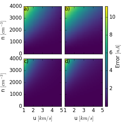
It is evident from Figure 8 that this method is robust for most of the plasma conditions around 67P. A smaller range of would reduce noise in the method, although instrumental noise provides a lower bound of the range of for a good fit to be found. Further errors might be introduced due to heavy fluctuations of the ion energy in a very dense plasma. As previously mentioned, we do not expect this method to be sensitive to . If anything it would mitigate the electron retardation current influence on our estimate, which we consider is our largest error source, due to the opposite sign and slope of the secondary electron current.