Tristability between stripes, up-, and down-hexagons and snaking bifurcation branches of spatial connections between up- and down-hexagons
Abstract
Third order amplitude equations on hexagonal lattices can be used for predicting the existence and stability of stripes, up- and down-hexagons in pattern forming systems. These amplitude equations predict the nonexistence of bistable ranges between up- and down-hexagons and tristable ranges between stripes, up- and down-hexagons. In the present work we use fifth order amplitude equations for finding such bistable and tristable ranges for a generalized Swift-Hohenberg equation and discuss stationary front connections between up- and down-hexagons.
I Introduction
It was shown by Turing [33] in 1952 that nonhomogeneous steady states arise in reaction-diffusion systems when a homogeneous state is unstable for the full system and stable for the kinetics. This discovery was followed by a large number of works, where systems of different scientific disciplines such as biology [13, 26], chemistry [27, 3, 40, 19, 21, 1], ecology [37, 24, 41, 23], and physics [32, 14] are studied for so-called Turing patterns.
Typical 2D Turing patterns are labyrinth patterns, gaps, and spots. If spots and gaps have a hexagonal structure, they are referred to as up- and down-hexagons, respectively. A special subset of labyrinth patterns are stripes. Stability transitions for such patterns are studied via third order amplitude equations in [15]. These amplitude equations predict that up- and down-hexagons corresponding to the same wavenumber cannot be stable at the same time. In contrast, tristable ranges between stripes, up-, and down-hexagons for a generalized Swift-Hohenberg model and for a specific system modeling vegetations of semiarid ecosystems are found in [16] and [24] via using numerical time integration, respectively. That tristable ranges between stripes, up-, and down-hexagons can be predicted using fifth order amplitude equations is shown in [16].
During the last 30 years, a great interest arose in localized Turing patterns. It was already understood by Pomeau [28] in 1986 that localized patterns on homogeneous backgrounds can be found in reaction-diffusion systems, when both corresponding states are stable. If the steady system has a spatial conserved quantity, it must necessarily be equal for both states in order to permit the existence of such a connecting state. The point where this takes place is called the Maxwell point. Via changing the wavelength of the patterned state, one can find more Maxwell points. As a consequence, branches of such states are found which move back and forth in parameter space and pass stable and unstable ranges. This scenario is referred to as snaking [39]. There are a lot of works, which investigate this effect over 1D domains (see e.g. [6, 7, 2]). For a detailed analysis using the Ginzburg-Landau formalism and beyond all order asymptotics see [8, 11].
Localized patterns correspond to two stationary fronts, which are glued together. Thus, such patterns exist on unbounded domains so that one cannot find these states on bounded domains. What remains are stationary states, which are periodic in space and for which the corresponding orbits pass near the homogeneous state and the Turing pattern. We also call such states localized or connecting patterns. Their branches also show a snaking behavior (see [4, 9, 10, 20, 17] for further details).
It was also understood by Pomeau [28] that stationary connections between hexagons and stripes should exist in ranges where both patterns are stable. The following connecting patterns are observed in [16] using numerical time integrations:
- (a)
localized patches of hexagons on a homogeneous background,
- (b)
connections between hexagons and stripes,
- (c)
connections between up- and down-hexagons.
Auto [12] is a software, which exists for a long time and which is often used for calculating solution branches of 1D patterns numerically and especially snaking branches. For a long time there was no software for performing these calculations for 2D patterns, which explains why numerically calculated branches of 2D patterns are rare. In [22] a custom continuation code was used for calculating snaking branches corresponding to states of type (a). Since a couple of years the software pde2path [34, 36] exists, which is designed for calculating solution branches of PDEs over 1D, 2D, and 3D domains. This software is used in [35, 38] for calculating branches corresponding to states of type (a) and (b). In the present work we also use this software for investigating branches of solutions of type (c), which has not been reported before.
The present work is organized as follows. We start with a quick review of third order amplitude equation reductions. After this we show a bifurcation diagram for which we used numerical continuation methods for following the stripe, gap, and spot branches bifurcating from a homogeneous state of the vegetation model mentioned above and observe a tristable range as well. In order to predict tristable ranges via the amplitude formalism we use a generalized Swift-Hohenberg equation, which is scaled with a parameter such that we are able to reduce the full equation to a system of fifth order amplitude equations. In the following a comparison of these predictions with numerical solutions is performed which shows that these amplitude equations give acceptable predictions if is small. At the end of the present work we show a snaking branch corresponding to connections between up- and down-hexagons and explain this behavior using conserved quantities.
II Third order amplitude equations
Consider
| (1) |
where , , a control parameter, , , space coordinates, and the time. Let be a homogeneous steady state of (1) and a Turing point with corresponding critical wavenumber . Using the ansatz
| (2) |
with , , , for , , and , we can reduce the full system to a system of amplitude equations given by
| (3) | ||||
(see [14, 18] for further details). By the center manifold reduction (see chapter 13 of [31]) an exists such that for all and
Such approximations are only valid near and for small amplitudes. Typical time independent solutions of (3) are up-hexagons , stripes , and down-hexagons for which the triple is given by , , , respectively. Here , , and . Their stability can be obtained from the Jacobian of (3). Unfortunately the amplitude reduction is only valid for small amplitudes (near ), and if the quadratic terms of the Taylor expansion of in (1) around are small.
Stability transitions between , , and via varying and are discussed in [15] and the following result is pointed out. For fixed parameters for which the three states , , and exist, the system (3) can only predict one of the following situations:
- •
only one of the states , , is stable (mono- stable case),
- •
and or are stable (bistable case),
- •
all three states are unstable.
Thus, bistable ranges between and and tristable ranges between , , and are not predictable using (3).
The following vegetation model for semi-arid ecosystems
| (4) | ||||
is discussed in [24] and used in [15] to apply the amplitude reduction and compare it with numerical results. Here , , and represent the vegetation density, ground water density, and precipitation, respectively. is used as a control parameter. The other parameters are given by
| (5) |
Please see [24] for modeling details and the meaning of these parameters. Numerical time integration methods are used in [24] to follow the stable parts of stripes and up- and down-hexagons by varying in both directions and to see where transitions between these patterns occur. Here, a very small tristable range between , , and is observed. In the present work we use numerical path following methods to calculate the corresponding branches and observe this tristable range as well (see Fig.1(a)). Furthermore, we use instead of and see that the tristable range is larger for this parameter set (see Fig.1(b)).
(a)

(b)

(c) Up-hexagons

(d) Stripes

(e) Down-hexagons

We also see in Fig.1 that the stripes bifurcate subcritically, turn around in a fold, and become stable after this fold. Since the amplitude equations (3) are only expanded up to third order terms, the fold and consequently the stable stripes cannot be described via (3). The parameter is changed in [15] such that both Turing points come closer together and stripes bifurcate supercritically, which makes the amplitude reduction valid for the whole existence regions of , , and .
III Fifth order amplitude equations
We have seen above that the third order amplitude equation reduction on a hexagonal lattice does not predict the tristability of , , and , but a tristable range for the reaction-diffusion system (4) is found numerically on bounded domains. In the present section we show that tristable ranges can be predicted via fifth order amplitude equations, which is also done in [16]. As for the third order case such an expansion is only valid for special systems for which the quadratic terms of the Taylor expansion of the kinetics around the homogeneous solution are small. Unfortunately this is not the case for (4) with the corresponding parameter set (5) so that we consider the following generalized Swift-Hohenberg equation
| (6) | ||||
with , , , , and .
(6) has the trivial solution which has a Turing bifurcation in . Furthermore, (6) is scaled with such that a fifth order amplitude equation reduction is possible and valid for small . To do so we use the ansatz (2) with and and end up with the following amplitude equation system (derived at )
| (7) | ||||
with for ,
and
To see if , , and are stable or not in their existence range, we split the amplitudes in (7) into real and imaginary parts and gain a system with 6 equations and thus a steady state of (7) has 6 eigenvalues. We fix and determine regions of stability depending on and (see Fig.2(a)). Besides monostable and bistable ranges between stripes and hexagons, we found tristable ranges between , , and and bistable ranges between and . We also fix and use pde2path for comparing analytical and numerical solutions, while is used as a control parameter (see Fig.2(b) and (c)).
(a)

(b)

(c)

Here we see that (7) gives reasonable predictions for . This does not hold for . Here the stripe branch bifurcates supercritically and has a fold in , where it turns around. This cannot be seen in Fig.2(c). We have some more folds on the branches corresponding to , , and , which cannot be predicted from (7). This shows that is too large for predicting hexagons and stripes well far away and near onset, but this example gives us other interesting results. Here we have ranges where two different stable types of the same pattern type exist (a small and large amplitude pattern). This holds for all three pattern types , , and . Thus, we find a range where the small and large amplitude down-hexagons, the zero-solution, the small and large amplitude stripes, and the large amplitude up-hexagons are multi-stable. And furthermore another range where the small and large amplitude down-hexagons, up-hexagons, and stripes are stable.
IV Spatial connections between patterns
In the present section we discuss spatial connections between up- and down-hexagons solving (6) with the parameter set used for creating Fig.2(b). We describe the behavior and the structure of the bifurcation diagram of such states, while we use the Ginzburg-Landau energy for explanations.
IV.1 Description
We use a domain, which is large in the -direction and small in the -direction, for finding stationary solutions connecting up- and down-hexagons in space. We calculate the branches corresponding to stripes, up- and down-hexagons on this domain and follow the branch which bifurcates in the point where the stripes lose their stability (see Fig.3). This branch is a mixed mode pattern connecting the stripe and up-hexagons branches. We call such states beans . They can also be found in (7) and are of the form with and . A density plot of a bean solution can be found in Fig.3(b).
(a)

(b) Solution on

(c) Solution 235

(d) left and right part of solution 235


There is a bifurcation point on the bean branch located near the stripe branch from which a snaking branch bifurcates (the gray branch of Fig.3(a)). The 235th solution on this branch is labeled in Fig.3(a) (we use the labels produced by pde2path) and shown in Fig.3(c). Here we can see that such a solution seems to be an orbit passing near up- and down-hexagons. It can be seen in Fig.3(c) and (d) that such a state changes its gap shape near the left boundary. This is because we use Neumann boundary conditions and a horizontal domain length of with ( is even).
We used (odd) for developing Fig.4 and Neumann boundary conditions. In this case stripes corresponding to the wavenumber have a maximum and minimum on the left and right boundary, respectively, or vice versa. Hexagons and beans corresponding to the wavenumber cannot fulfill the boundary conditions, but a state, which passes near up- and down-hexagons such as solution 235 of Fig.3, does. When the stripe branch loses its stability, it does not bifurcate a bean branch, but a branch like the gray one of Fig.3(a).
(a)

(b) Stripe solution

(c) 53

(e) 80

(f) 120

(g) 410

(h) 458

(i) 810

(j) left and right part of 458


We describe the behavior of this branch in the following. A formation of a spot occurs on the left side (from bifurcation to solution 53). Then the branch turns around in a fold in the point, where stripes become stable. It follows a part where a gap front invades the stripes along the branch. Solution 80 is a state which is a mix of stripes, up-, and down-hexagons. Solution 120 consists of up- and down-hexagons and an interface which lies on the left side. It follows a part of the branch where it moves back and forth in parameter space by passing stable and unstable ranges (snaking). Along this snake the interface moves to the right side (the up-hexagons invade the down-hexagons). The interface shift is of the length from a fold on one side to the fold after next on the same side (compare solution 410 and 458). Because of the boundary problems described above the branch cannot go back to the spot branch as the gray branch of Fig.3(a) does, but terminates in a branch which is nearby (see solution 810). In Fig.4(j) we can see that we have no boundary problems for connections between up- and down-hexagons as we had in Fig.3. Furthermore, one should mention that the gray branches of Fig.3 and Fig.4 show a similar behavior. The length of the snake in Fig.4 is larger than the one of Fig.3, which is because we used a larger domain here.
IV.2 Explanations via conserved quantities
In the following we explain the behavior of the gray branches of Fig.3 and Fig.4 analytically via amplitude equations and Ginzburg-Landau energy techniques (see [22, 35]) and numerically via the full system and the Hamiltonian (see [22]). We start with the first way. The amplitude reduction (7) is a Landau system of the form
where is time dependent. Assuming that is also space dependent we obtain the Ginzburg-Landau system
| (8) | ||||
Background on this formal procedure and for so called attractivity and approximation theorems can be found in [29, 5, 30, 25, 31].
Restricting to real amplitudes , we can split the total energy into the kinetic and potential energy, i.e., , where
| (9) |
with
and
The Hamiltonian for stationary states of generalized Swift-Hohenberg equations over 2D domains can be found in [22]. For (6) this Hamiltonian is given by
| (10) | ||||
with
| (11) |
It holds and , i.e., and are conserved. Thus, a necessary conditions for a heteroclinic front connection between two stationary states in (8) and (6) is that both have the same potential energy and Hamiltonian , respectively. Using the Ginzburg-Landau energy is an easy and rapid way, but is only valid near onset. Using the Hamiltonian is more costly, but gives accurate results not only near onset.
(a)

(b)
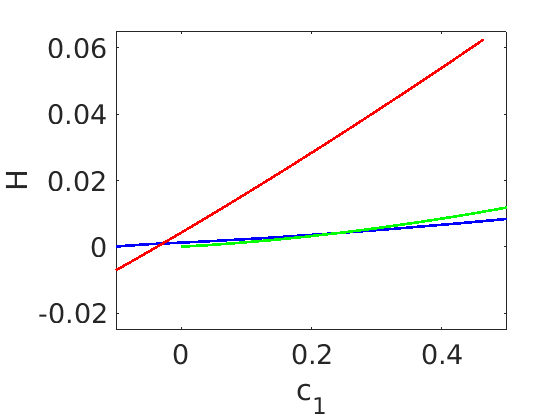
The potential energy (9) and the Hamiltonian (10) for stripes, up-, and down-hexagons are shown in Fig.5(a) and (b), respectively. First of all we can see that up- and down-hexagons have the same potential energy and Hamitonian for , which explains the existence of connections between up- and down-hexagons in this range. Furthermore, we can conclude that the state 53 on the gray branch of Fig.4 is not a state for which the corresponding orbit passes near stripes and up-hexagons, but we expect that the orbit moves from stripes into the spot direction and is never close to up-hexagons before moving back to stripes.
Stripes and up-hexagons have the same potential energy and Hamitonian for such that a necessary condition for the existence for a connection between stripes and up-hexagons is fulfilled. We did not try to find such a state for studying the snaking behavior of the branch, since this is already done in [35, 38] for other systems and we do not expect to find a different behavior. But what we can see is that the invasion of down-hexagons between solution 80 and 120 starts when the potential energy of stripes becomes smaller than the one of down-hexagons.
V Conclusion
We cannot predict bistable ranges between up- and down-hexagons and tristable ranges between stripes, up- and down-hexagons if we use a third order amplitude reduction for pattern forming systems. If we use fifth order amplitude reductions, we are able to find such ranges. We studied a generalized Swift-Hohenberg equation (6) which is scaled with a parameter , which makes a fifth order amplitude reduction easy and valid for small . We fixed for finding tristable ranges between stripes, up- and down-hexagons in the --plane based on the amplitude reduction. We fixed and used as bifurcation parameter for calculating branches of stripes, up- and down-hexagons for and using numerical path following methods. We compared these branches with the one obtained from the amplitude reductions and saw that we obtain acceptable predictions for and a completely different bifurcation diagram for . Here we found ranges, where five different states are stable.
We went on with for finding interesting states existing in the multistable ranges and found a snaking branch of connections between up- and down-hexagons. This branch bifurcates from the stripe branch and terminates on the spot branch. We used conserved quantities in order to understand the location of the snaking part.
References
- [1] T. Bánsági, V. K. Vanag, and I. R. Epstein. Tomography of Reaction-Diffusion Microemulsions Reveals Three-Dimensional Turing Patterns. Science, 331(6022):1309–1312, March 2011.
- [2] M. Beck, J. Knobloch, D.J.B. Lloyd, B. Sandstede, and T. Wagenknecht. Snakes, ladders, and isolas of localized patterns. SIAM J. Math. Anal., 41(3):936–972, 2009.
- [3] I. Berenstein, L. Yang, M. Dolnik, A. M. Zhabotinsky, and I. R. Epstein. Superlattice Turing structures in a photosensitive reaction-diffusion system. Physical review letters, 91(5):058302, 2003.
- [4] A. Bergeom, J. Burke, E. Knobloch, and I. Mercader. Eckhaus instability and homoclinic snaking. Phys.Rev.E, 78:025201, 2008.
- [5] P. Bollermann, A. van Harten, and G. Schneider. On the justification of the Ginzburg–Landau approximation. In A. Doelman and A. van Harten, editors, Nonlinear dynamics and pattern formation in the natural environment, pages 20–37. Longman UK, 1995.
- [6] J. Burke and E. Knobloch. Localized states in the generalized Swift-Hohenberg equation. Phys. Rev. E, 73:056211, May 2006.
- [7] J. Burke and E. Knobloch. Homoclinic snaking: Structure and stability. Chaos, 17(3):037102, 15 p., 2007.
- [8] S.J. Chapman and G. Kozyreff. Exponential asymptotics of localised patterns and snaking bifurcation diagrams. Physica D, 238(3):319–354, 2009.
- [9] J. Dawes. Localized pattern formation with a large-scale mode: Slanted snaking. SIAM J. Appl. Dyn. Syst., 7(1):186–206, 2008.
- [10] J. Dawes. Modulated and localized states in a finite domain. SIAM J. Appl. Dyn. Syst., 8(3):909–930, 2009.
- [11] A.D. Dean, P.C. Matthews, S.M. Cox, and J.R. King. Exponential asymptotics of homoclinic snaking. Nonlinearity, 24(12):3323–3351, 2011.
- [12] E.J. Doedel, A.R. Champneys, T.F. Fairgrieve, Y.A. Kuznetsov, B. Sandstede, and X.-J. Wang. AUTO97: Continuation and bifurcation software for ordinary differential equations. Available by FTP from ftp.cs.concordia.ca, 1997.
- [13] A. Gierer and H. Meinhardt. A theory of biological pattern formation. Biological Cybernetics, 12(1):30–39, December 1972.
- [14] M. Golubitsky, J. W. Swift, and E. Knobloch. Symmetries and pattern selection in Rayleigh-Bénard convection. Physica D: Nonlinear Phenomena, 10(3):249–276, 1984.
- [15] K. Gowda, H. Riecke, and M. Silber. Transitions between patterned states in vegetation models for semiarid ecosystems. Phys. Rev. E, 89:022701, Feb 2014.
- [16] M. F. Hilali, S. Métens, P. Borckmans, and G. Dewel. Pattern selection in the generalized Swift-Hohenberg model. Phys. Rev. E, 51:2046–2052, Mar 1995.
- [17] S. M. Houghton and E. Knobloch. Homoclinic snaking in bounded domains. Phys.Rev.E, 80:026210, 2009.
- [18] R.B. Hoyle. Pattern formation. Cambridge University Press., Cambridge, UK, 2006.
- [19] H. Katsuragi. Diffusion-induced spontaneous pattern formation on gelation surfaces. EPL (Europhysics Letters), 73(5):793, 2006.
- [20] G. Kozyreff, P. Assemat, and S.J. Chapman. Influence of boundaries on localized patterns. Phys. Rev. Letters, 103:164501, 2009.
- [21] M. Leda, V. K. Vanag, and I. R. Epstein. Instabilities of a three-dimensional localized spot. Physical Review E, 80(6):066204, 2009.
- [22] D.J.B. Lloyd, B. Sandstede, D. Avitabile, and A.R. Champneys. Localized hexagon patterns of the planar Swift-Hohenberg equation. SIAM J. Appl. Dyn. Syst., 7(3):1049–1100, 2008.
- [23] A. Manor and N. M. Shnerb. Dynamical failure of turing patterns. EPL (Europhysics Letters), 74(5):837, 2006.
- [24] E. Meron, E. Gilad, J. von Hardenberg, M. Shachak, and Y. Zarmi. Vegetation patterns along a rainfall gradient. Chaos, Solitons, and Fractals, 19(2):367 – 376, 2004. Fractals in Geophysics.
- [25] A. Mielke. The Ginzburg-Landau equation in its role as a modulation equation. In Handbook of dynamical systems, Vol. 2, pages 759–834. North-Holland, 2002.
- [26] J.D. Murray. Mathematical biology. Springer-Verlag, Berlin, 1989.
- [27] B. Peña and C. Pérez-García. Selection and competition of turing patterns. EPL (Europhysics Letters), 51(3):300, 2000.
- [28] Y. Pomeau. Front motion, metastability and subcritical bifurcations in hydrodynamics. Physica D, 23:3–11, 1986.
- [29] G. Schneider. Error estimates for the Ginzburg–Landau approximation. ZAMP, 45:433–457, 1994.
- [30] G. Schneider. Global existence results in pattern forming systems – Applications to 3D Navier–Stokes problems –. J. Math. Pures Appl., IX, 78:265–312, 1999.
- [31] G. Schneider and H. Uecker. Nonlinear PDE – a dynamical systems approach, volume 182 of Graduate Studies Mathematics. AMS, 2017.
- [32] J. Swift and P. C. Hohenberg. Hydrodynamic fluctuations at the convective instability. Physical Review A, 15(1):319, 1977.
- [33] A. M. Turing. The chemical basis of morphogenisis. Philosophical transaction of the Royal Society of London - B, 237:37–72, 1952.
- [34] H. Uecker. www.staff.uni-oldenburg.de/hannes.ue cker/pde2path, 2017.
- [35] H. Uecker and D. Wetzel. Numerical Results for Snaking of Patterns over Patterns in Some 2D Selkov-Schnakenberg Reaction-Diffusion Systems. SIAM J. Appl. Dyn. Syst., 13(1):94–128, 2014.
- [36] H. Uecker, D. Wetzel, and J. Rademacher. pde2path – a Matlab package for continuation and bifurcation in 2D elliptic systems. NMTMA, 7:58–106, 2014.
- [37] J. von Hardenberg, E. Meron, M. Shachak, and Y. Zarmi. Diversity of vegetation patterns and desertification. Phys. Rev. Lett., 87:198101, Oct 2001.
- [38] D. Wetzel. Pattern analysis in a benthic bacteria-nutrient system. Math. Biosci. Eng., 13(2):303–332, 2016.
- [39] P.D. Woods and A.R. Champneys. Heteroclinic tangles and homoclinic snaking in the unfolding of a degenerate reversible Hamiltonian-Hopf bifurcation. Physica D, 129(3-4):147–170, 1999.
- [40] L. Yang, M. Dolnik, A. M. Zhabotinsky, and I. R. Epstein. Turing patterns beyond hexagons and stripes. Chaos: An Interdisciplinary Journal of Nonlinear Science, 16(3):037114, 2006.
- [41] H. Yizhaq, E. Gilad, and E. Meron. Banded vegetation: biological productivity and resilience. Physica A: Statistical Mechanics and its Applications, 356(1):139–144, 2005.