Nodal portraits of quantum billiards: Domains, lines, and statistics

A dynamical system is termed as integrable in the sense of Liouville-Arnold [27] if there are $f$ constants of motion for a system with $f$ degrees of freedom. These constants must be functionally independent and in involution. Furthermore, the vector fields have to remain regular everywhere in phase space. A circular billiard (Fig. 4, $f=2$) is an example of this type, where the total energy $E$ and the angular momentum $L$ are conserved. Since the system is integrable, the distance between two “nearby” trajectories increases linearly with time. For any generic system with two degrees of freedom, one can find action-angle variables $(I_{1},I_{2},\theta_{1},\theta_{2})$ by employing an appropriate generating function [393]. There are two canonical frequencies, $\omega_{i}=\mathrm{d}\,\theta_{i}/\mathrm{d}\,t$, $i=1,2$, which are functions of phase-space variables for a nonlinear system. In exceptional situations (called nonlinear resonances), the ratio of these two frequencies becomes a rational number and certain regions in phase space are endowed with a chain of islands. Each island has at its center an elliptic point (stable equilibrium), and a separatrix connecting hyperbolic points. The invariant tori are broken, and new intricate structures are formed (see, for example, Berry [95]). Such systems are said to be quasi-integrable. However, there exists another qualitatively different class of behavior demonstrated by most billiards. Consider the cardioid billiard of Fig. 4; now, the only constant of motion is the total energy $E$. Classically, the motion on the billiard table is irregular and unpredictable, displaying extreme sensitivity to initial conditions. More importantly, the separation between neighboring trajectories grows exponentially with time with a divergence characterized by the Lyapunov exponent. The cardioid billiard is therefore chaotic. A “typical” billiard is expected to be non-integrable [520] and most of these are believed to be chaotic, possessing a positive Kolmogorov-Sinai entropy [147].

Clearly, this trajectory-centric distinction between order and chaos does not hold in the quantum regime. Moreover, since the Schrödinger equation is linear, there is no scope for chaos in the conventional sense.³³ 3 Hence, the widely prevalent usage of the term “quantum chaos”, which just connotes the quantum mechanics of classically chaotic systems, should always be taken with a grain of salt. However, the latent classical dynamical properties do leave their imprints on the statistical behavior of eigenvalues. The statistics of the energy levels of a generic integrable system can be characterized by a Poissonian random process [108]. Conversely, the energy-level statistics of fully chaotic systems are described by the eigenvalues of random matrices obeying appropriate symmetries [133, 478, 419]. For quasi-integrable systems, the statistics can be modeled as a superposition of Poisson and Wigner distributions with weights proportional to the relative fractions of regular and chaotic subregions [104]. Of course, as always, exceptions abound: prominent counterexamples include arithmetic systems [41, 128, 136, 135, 503] and quantized cat maps [331, 275].

The classical dynamics of the billiard is also betokened by the structure of the eigenfunctions themselves. The semiclassical eigenfunction hypothesis [584, 585, 586, 91, 97] asserts that the eigenstates should concentrate on those regions which a generic orbit explores in the long–time limit. This statement is best formulated in terms of the Wigner function $W\,(p,q)$, which is a phase-space representation of the wavefunction [611]. In integrable systems, the motion remains confined to invariant tori in phase space—so $W\,(p,q)$ should localize on these tori in the semiclassical limit—whereas in ergodic systems, the whole energy surface is filled in a uniform manner and $W\,(p,q)$ is expected to semiclassically condense on the energy shell as $W\,(p,q)\sim[1/V(\Sigma_{E})]\,\delta(H\,(p,q)-E)$, where $H$ is the Hamiltonian and $V(\Sigma_{E})$ is the volume of the shell set by $H\,(p,q)=E$ [49]. For the latter class, this was established to be equivalent to the quantum ergodicity theorem [517, 621, 581, 281, 243, 628]—which states that “most” eigenstates are equidistributed in the semiclassical limit—by Bäcker et al. [49], Bäcker et al. [48]. Written in position space, this implies

$$\lim_{j\rightarrow\infty}\int_{\mathscr{R}}\,\lvert\psi_{n_{j}}(\mathbf{r})\rvert^{2}\,\mathrm{d}\mathbf{r}=\frac{\mathrm{vol}\,(\mathscr{R})}{\mathrm{vol}\,(\mathcal{D})}$$

(5)

for a subsequence $\{\psi_{n_{j}}\}\subset\{\psi_{n}\}$ of density one. Thus, as $E\rightarrow\infty$, the probability of finding a particle in a certain region of the billiard $\mathscr{R}\subset\mathcal{D}$ is identical to that for the classical system, for almost all eigenfunctions. This consonance is pictorially conveyed by Fig. 4.

The phase space representation of eigenfunctions of integrable systems reveals a direct correspondence with the underlying periodic orbits. As the degree of nonintegrability increases, the eigenfunctions become progressively more structured. For chaotic systems, the eigenfunctions often evince an “anomalous enhancement or suppression of eigenstate intensity on or near an unstable periodic orbit and its invariant manifolds” [326], over and beyond the statistically expected density. Discovered by McDonald and Kaufman [416] and christened “scarring” by Heller [283], this observation is notably distinct from the attraction of eigenstate intensity associated with stable classical orbits, the latter being due to reasons well-understood by a purely semiclassical theory of integrable systems [107, 106, 622]. Quantitatively, scarring was partially accounted for on the basis of wavepacket dynamics in Husimi phase space [283], coordinate space [124] and Wigner phase space [98, 99]. At a more formal level, a rigorous explanation was tendered by Fishman et al. [217] in their use of the Fredholm method to derive a semiclassical formula for scar strengths that had previously been obtained using Riemann-Siegel resummation techniques [4, 3, 2]. Although the scars themselves do not disappear in the semiclassical limit [327], the scarred area of phase space (surrounding the orbit), and hence the total weight of the scar, vanishes as $\hbar\rightarrow 0$. One could equally well look for “strong scarring” [489] in the semiclassical limit—this necessitates the convergence of the total weight of the wavefunction on the unstable orbit [326]. However, this property has not been found to hold for any physical system thus far and its existence has even been explicitly disproved for certain arithmetic hyperbolic manifolds.⁴⁴ 4 Moreover, the semiclassical defect measures, to adopt mathematical parlance, cannot be a finite sum of delta functions on closed geodesics on compact Reimannian $C^{\infty}$ manifolds with Anosov flow and the high-energy eigenfunctions are thus, at least, “half-delocalized” [18, 17].

Incidentally, addressing quasi-integrable or mixed systems, Keating and Prado [334] found that the probability density for perturbed cat maps is localized strongly around the bifurcated periodic orbits—the phenomenon was homologously styled “superscarring”.

Liouville-Arnold integrability is easily broken, when, for instance, the vector fields become singular without disturbing other conditions of integrability. Such dynamical systems are titled pseudointegrable, named thus by Richens and Berry [481]. Nonintegrable polygonal billiards are pseudointegrable; they are also non-chaotic insofar as the Lyapunov exponent is zero.⁵⁵ 5 A finite-time exponent can also be defined for polygonal billiards as suggested by Moudgalya et al. [433]. In this regard, we now turn to a billiard in a polygon $\mathcal{Q}\subset\mathbb{R}^{2}$ where all angles are commensurate with $\pi$ [629]. Let us fix a direction $\hat{e}$, say, along one of the sides of ${\mathcal{Q}}$. One can write the angles between $\hat{e}$ and the remaining sides in the form $\alpha_{r}=\pi\,m_{r}/2\,n_{r}$ with $r=1,2,\ldots$. Furthermore, let $N=N({\mathcal{Q}})$ denote the least common denominator of the fractions $m_{r}/n_{r}$. It was observed that the function

$\displaystyle F(x,y,p_{x},p_{y})=F(\phi)=\lvert\phi\rvert\,\mathrm{mod}\,\frac{\pi}{N}$

(6)

is well-defined on the energy surface ${\mathcal{M}}$ and invariant with the phase-space flow. For a given $c\in[0,\pi/2N]$, there is an invariant subset ${\mathcal{M}}_{c}$ of ${\mathcal{M}}$. If $c\notin\{0,\,\pi/2N\}$, then the set ${\mathcal{M}}_{c}$ is obtained by pairwise identification of the sides of $4N$ non-intersecting copies of the polygon labelled by $\phi_{s}^{\pm}=\pm c+s\,\pi/N$, with $s=0,1,\ldots,(2N-1)$. The identification of the sides is dictated, once again, by Snell’s law. Zemlyakov and Katok [629] proved that ${\mathcal{M}}_{c}$ is a two-dimensional manifold of genus $g>1$ depending on the shape of the polygon. The fact that the motion in phase space is not restricted to a torus as for integrable systems but rather, to a surface with a more complicated topology, is conveyed by the moniker pseudointegrable. A prototypical example is the $(\pi/3,2\pi/3)$-rhombus billiard, illustrated in Fig. 5.

The statistical properties of the eigenvalues of classically pseudointegrable quantum billiards have been numerically established [129, 606, 115] to be intermediate between those of regular and chaotic systems. The wavefunctions are also equally intriguing, demonstrating pronounced scarring behavior that can be related to families of periodic orbits [131]. For example, many of the solutions to the Schrödinger equation for the rhombus billiard [115] exhibit significantly enhanced intensities in the close neighborhood of a periodic orbit. However, in contrast to chaotic systems, these scar structures persist even at large quantum numbers, thereby earning the epithet “superscars”. Experimentally, superscarring (Fig. 6) has been observed in microwave billiards [126, 483] and LiNC $\leftrightharpoons$ LiCN isomerization reactions [474]. In many-body systems, it is often the case that the amplitude of a collective excitation is spread over states forming the background, well-known examples being the giant dipole resonances in nuclei [134, 536] and metallic clusters [139]. The distinctly created excitation acts as a “doorway” to the background states. Analogously, a superscar of a pseudointegrable billiard also spreads over a large number of non-scarred wavefunctions. This convenient parallel enables the modeling of doorway states in the quantum spectra of nuclei [1].

The nodal lines of Chladni’s vibrating plates are a window to a deeper theory—of vortices—that, paradoxically, neither Chladni nor anyone else ever witnessed in the motion of plates [179]. A direct (theoretical) route to observe the emergence of vortices is to study the displacement of the plate $A\,(x,y,t)$ from its equilibrium position, near the nodal lines. As with any wave phenomenon, it is convenient to regard the actual displacement as the real part of a complex amplitude $u(x,y)\,\exp\,(\mathrm{i}\,\omega\,t)$. In the immediate neighborhood of a nodal line along the $x$-axis, the complex field is $u^{(x)}(x,y)=y$; similarly, $u^{(y)}(x,y)=x$ for a nodal line along $\hat{y}$. The displacements, pictured in Fig. 7, pivot about these lines as time evolves. Now, consider two frequency-degenerate eigenmodes with nodal lines in the $\hat{x}$ and $\hat{y}$ directions, which are locally described as above—obviously, these orthogonal lines cross each other at a point, somewhere on the plate. It is interesting to inspect the ensuing oscillation structures in the vicinity of the intersection point for a linear superposition of the eigenstates. If the complex fields are simply summed up as

$$u\,(x,y)=x+y$$

(7)

the resultant eigenmode displays a nodal line, inclined at 45^∘ to the two axes. Alternatively, if the fields are added out of phase by $\pi/2$,

$$u\,(x,y)=x+\mathrm{i}\,y,$$

(8)

then the amplitude field $A$ does not merely pivot about a new nodal line but instead, rotates around the crossing point, thus engendering a vortex (at the intersection point). On retracing Chladni’s steps, these vortices should, in principle, be visible as fine islands of sand.

As early as 1931, Dirac [196] demonstrated that nodal points give rise to current vortices. Vortices, in the most general sense, refer to singular points at which the phase of a field becomes undefined. They are commonplace in physical fields of at least two variables, where the physical quantity signified by the field can be naturally represented in a plane [189], such as the Argand plane or $\mathbb{R}^{2}$. In particular, the field could be the wavefunction for an open quantum billiard, or one with broken time-reversal symmetry—in either case, $\psi$ acquires a finite imaginary part. It could also just as well be the complex order parameter of a superconductor or a scalar optical field. Consider a generic complex scalar wave

$$\psi\,(\mathbf{r},t)=\xi\,(\mathbf{r},t)+\mathrm{i}\,\eta\,(\mathbf{r},t)=\rho\,(\mathbf{r},t)\,\exp\,\left\{\mathrm{i}\,\chi\,(\mathbf{r},t)\right\}$$

(9)

with $\xi,\,\eta,\,\rho,\,\chi\in\mathbb{R}$. All is well with this representation, except at the nodal points where $\psi$ (and consequently, the intensity $=\rho^{2}$) is zero. Just as the angle of polar coordinates is ill-defined precisely at the origin, along loci of vanishing $\rho$, the phase $\chi$ is indeterminate. These phase singularities—also called optical vortices—were first illustrated by Nye and Berry [447] as dislocations of wavefronts and later, investigated by Berry [96], Berry [100], Nye [446]. The dislocations reside on the contour lines of intersection of the two surfaces

$$\xi\,(\mathbf{r},t)=0,\hskip 7.11317pt\eta\,(\mathbf{r},t)=0$$

(10)

as seen in Fig. 8; we call these lines $\xi$NL and $\eta$NL, respectively. To borrow Berry and Dennis’ [2000] eloquent description, “in light, they are lines of darkness; in sound, threads of silence.” Unfortunately, the nodal lines $\xi$NL and $\eta$NL, being dependent on the overall phase of the wavefunction, are hardly uniquely defined. The nodal points, on the contrary, are invariant under a phase transformation of the wave function and remain unmoved in space on multiplying $\psi$ by an (arbitrary) constant phase factor $\exp\,(\mathrm{i}\,\alpha)$ [86]. This makes them of greater utility when attempting to characterize a complex chaotic wave function.

Around a vortex, the phase assumes all possible values in its $2\pi$ range, leading to a circulation of the wave energy. Although the change in $\chi$ is usually nonuniform [430], upon traversing a closed circuit $\gamma$ enclosing the phase-singular point, there is a net change of phase

$$Q=\frac{1}{2\pi}\oint\mathrm{d}\,\mathbf{r}\cdot\nabla\chi=\frac{1}{2\pi}\oint_{\gamma}\mathrm{d}\,\chi,$$

(11)

which is quantized in units of $2\,\pi$. The integer $Q$ is referred to as the strength or topological charge [274] and $\mathscr{S}=\mathop{\mathrm{sgn}}\,(Q)$, which is positive if the phase increases in a right-handed sense, is colloquially termed the sign of the singularity. In the language of Eqs. (7, 8), the complex field near the center of a canonical charge-$Q$ vortex located at the origin takes the form [427]

$$u\,(x,y)=(x+\mathrm{i}\,y)^{\,\lvert Q\rvert}=\exp\,(\mathrm{i}\,Q\,\phi).$$

(12)

Higher-charge vortices with $Q>1$ (Fig. 7), however, are non-generic in that they are not stable with respect to perturbations [231], which split a charge-$Q$ vortex into $\lvert Q\rvert$ vortices of charge $\pm 1$ [179].

Associated with the field $\psi$ is a current

$$\mathbf{j}=\mathop{\mathrm{Im}}\,\left(\psi^{*}\,\nabla\psi\right)=\xi\,\nabla\eta-\eta\,\nabla\xi=\rho^{2}\,\nabla\chi.$$

(13)

This is the usual quantum-mechanical probability current density. In electrodynamics [311], $\mathbf{j}$ is the familiar Poynting vector if $\psi$ stands for a polarized (scalar) component of the electric field. Since $\mathbf{j}$ is aligned along the gradient $\nabla\chi$, i.e., in the direction of change of phase, phase singularities constitute vortices of the optical current flow [189]. The corresponding vorticity is defined as

$$\mathbf{\Omega}=\frac{1}{2}\nabla\times\mathbf{j}=\frac{1}{2}\mathop{\mathrm{Im}}\,\left(\nabla\psi^{*}\times\nabla\psi\right)=\nabla\xi\times\nabla\eta.$$

(14)

The vector $\mathbf{\Omega}$, being perpendicular to the normals to the two surfaces in Eq. (10), points along the dislocation line. In three dimensions, the total length of dislocation line in a volume $\mathcal{V}$ is

$$L(\mathcal{V})=\int_{\mathcal{V}}\mathrm{d}\,\mathbf{r}\,\,\delta\,(\xi)\,\delta\,(\eta)\,\lvert\Omega(\mathbf{r})\rvert,$$

(15)

whereby we can calculate the dislocation line density. For the time being, however, let us focus on a unit topological charge in one lower dimension. This simplifies life, and Eqs. (11, 13), a little, whereupon

	$\displaystyle Q$	$\displaystyle=\mathop{\mathrm{sgn}}\,(\mathbf{\Omega}\cdot\hat{z})=\mathop{\mathrm{sgn}}\left(\xi_{x}\,\eta_{y}-\xi_{y}\,\eta_{x}\right),$		(16)
	$\displaystyle\mathbf{j}$	$\displaystyle=\left(\xi\,\eta_{x}-\eta\,\xi_{x},\,\xi\,\eta_{y}-\eta\,\xi_{y}\right),$		(17)

the subscripts indicating partial derivatives. Note that the strength $Q$ is now identical to the sign $\mathscr{S}$—also called the winding number (WN)—that defines the sense of circulation of the current swirling about the vortex. Neighboring nodal points on the same nodal line (either $\xi$NL or $\eta$NL) always have opposite WNs [86] and generically, any nearest neighbors are strongly anticorrelated in sign [518]. In fact, the sign of any single vortex in a random Gaussian wave field determines the sign of all other vortices in the field.

The current is zero at both vortices, where $\psi=\xi=\eta=0$, and saddle points (stagnation points in the flow), where $\xi/\eta=\xi_{x}/\eta_{x}=\xi_{y}/\eta_{y}$ [297]. To tell them apart,⁶⁶ 6 In conventional mathematical nomenclature, vortices (saddles) are the elliptic (hyperbolic) points in the flow. we scrutinize the Jacobian

$$\mathcal{J}=\partial_{x}\,j_{x}\,\,\partial_{y}\,j_{y}-\partial_{y}\,j_{x}\,\,\partial_{x}j_{y},$$

(18)

which is positive at vortices but negative at saddles. As a consequence of $\psi$ satisfying the Helmholtz equation, $\mathcal{J}$ neatly separates into two parts

$$\mathcal{J}=\mathcal{J}_{v}-\mathcal{J}_{s},$$

(19)

with the individual contributions

	$\displaystyle\mathcal{J}_{v}$	$\displaystyle\equiv\left(\xi_{x}\,\eta_{y}-\xi_{y}\,\eta_{x}\right)^{2},$		(20)
	$\displaystyle\mathcal{J}_{s}$	$\displaystyle\equiv\frac{1}{2}\left[\left(\xi\,\eta_{xx}-\eta\,\xi_{xx}\right)^{2}+\left(\xi\,\eta_{yy}-\eta\,\xi_{yy}\right)^{2}\right]$
		$\displaystyle+\left(\xi\,\eta_{xy}-\eta\,\xi_{xy}\right)^{2}.$		(21)

From the general density of critical points

$$D_{\mathrm{crit}}(\mathbf{r})=\hskip-7.11317pt\sum_{\{\mathbf{r}^{\prime}:\,\mathbf{j}(\mathbf{r}^{\prime})=0\}}\hskip-7.11317pt\delta^{2}(\mathbf{r}-\mathbf{r}^{\prime})=\delta^{2}\left(\mathbf{j}\,(\mathbf{r})\right)\,\lvert\mathcal{J}(\mathbf{r})\rvert,$$

(22)

it is now easy to compute the saddle and vortex densities [102, 494, 187],

	$\displaystyle D_{s}(\mathbf{r})$	$\displaystyle=\delta^{2}\left(\mathbf{j}\,(\mathbf{r})\right)\mathcal{J}_{s}(\mathbf{r}),$		(23)
	$\displaystyle D_{v}(\mathbf{r})$	$\displaystyle=\delta^{2}\left(\mathbf{j}\,(\mathbf{r})\right)\mathcal{J}_{v}(\mathbf{r})=\delta\,(\xi)\,\delta\,(\eta)\,\lvert\xi_{x}\,\eta_{y}-\xi_{y}\,\eta_{x}\rvert,$

respectively. $D_{v}$, which can be determined statistically (at least, in the mean), specifies the dislocation point (or vortex) density—the mean number of dislocation lines piercing unit area of a plane [92]. These statistics have been thoroughly studied for quasimonochromatic paraxial waves [60], monochromatic waves in two dimensions [234, 233, 230, 229, 232, 235, 519], isotropic random waves [102], and random waves subject to the Aharonov-Bohm effect [301] among others, with novel extensions to the statistics of knotted nodal lines by Taylor and Dennis [560], Taylor and Dennis [561].

Closer to the theme of our discussion, vortices were predicted in eigenfunctions of highly symmetric billiards [165, 163, 164] and their telltale fingerprints have been spotted in closed, microwave cavities, coherently excited at multiple points [185]. Similar predictions [105] and experiments [169, 62, 86, 451, 493] were proffered for quantum billiards without time-reversal symmetry, and more recently, for open billiards [357]. On the optical physics front too, phase singularities have generated considerable enthusiasm, in part due to their connections with beams carrying orbital angular momentum [119, 12, 13, 565, 280, 525, 239, 452], which fueled remarkable experiments [330, 74, 450, 449] seeking to actively create and annihilate optical dislocations in laser fields. However, as fascinating as the physics thereof may be, we wouldn’t want to let our focus stray too far from nodal domains, to which we now thus return.

Even without inspecting the eigenfunctions, important information about the domain $\mathcal{D}$ can be gleaned from the eigenvalues alone as we demonstrate in this subsection. For the sake of brevity and continuity, we refrain from presenting detailed proofs; instead, we simply state the relevant results, the emphasis being on their underlying physics.

A good point to start is the variational formulation of the eigenvalue problem which owes itself to the minimax principle [178]

	$\displaystyle\lambda_{j}$	$\displaystyle=\frac{\lvert\lvert\nabla u_{j}\rvert\rvert^{2}_{L_{2}\,(\mathcal{D})}+h\,\lvert\lvert u_{j}\rvert\rvert^{2}_{L_{2}\,(\partial\,\mathcal{D})}}{\lvert\lvert u_{j}\rvert\rvert^{2}_{L_{2}\,(\mathcal{D})}},$		(33)
		$\displaystyle=\min\max\frac{\lvert\lvert\nabla v\rvert\rvert^{2}_{L_{2}\,(\mathcal{D})}+h\,\lvert\lvert v\rvert\rvert^{2}_{L_{2}\,(\partial\,\mathcal{D})}}{\lvert\lvert v\rvert\rvert^{2}_{L_{2}\,(\mathcal{D})}},$		(34)
		$\displaystyle=\min\max{\displaystyle\frac{{\displaystyle\int}_{\mathcal{D}}\left[\bigg({\displaystyle\frac{\partial v}{\partial x}}\bigg)^{2}+\bigg({\displaystyle\frac{\partial v}{\partial y}}\bigg)^{2}\right]\mathrm{d}{\bf x}\,\,\mathrm{d}{\bf y}}{{\displaystyle\int_{\mathcal{D}}v^{2}\,\,\mathrm{d}{\bf x}\,\mathrm{d}{\bf y}}}}\textrm{ for }d=2,$

where the maximum is over all linear combinations of the form

$$v=a_{1}\,u_{1}+a_{2}\,u_{2}+\cdots+a_{j}\,u_{j},$$

and the minimum is over all choices of $j$ linearly independent continuous and piecewise-differentiable functions $u_{1},\,u_{2},\,\ldots,\,\,u_{j}$ [288]; this space of functions is often termed the Sobolev space $H^{1}(\mathcal{D})$. While on the subject of terminology, we add that the ratio of quadratic forms in the third equality is known as the Rayleigh quotient. Although Eq. (34) looks cumbersome, simplification immediately follows for both Dirichlet and Neumann boundary conditions. It is easy to recognize that the second term in the numerator of Eq. (34) vanishes with these conditions; in the former case, $v$ itself is zero on the boundary $\partial\,\mathcal{D}$ whereas for the latter, $h=0$. In addition to its mathematical elegance, the minimax principle has other important consequences like the Rayleigh-Ritz method for obtaining upper bounds for eigenvalues. The Rayleigh-Ritz method has also been used to estimate the eigenvalues of the Laplacian for rhombical [114, 600] and parallelogram [206] regions. For a more detailed discussion about the numerical aspects of this connection, the curious reader is directed to Ch. 12 of [363].

Another significant implication of the minimax principle is the property of domain monotonicity for Dirichlet boundary conditions, i.e., eigenvalues monotonously decrease when the domain is enlarged. To see this, consider a region $\mathcal{D}$ that is properly contained in $\mathcal{D}^{\prime}$; a set of admissible eigenfunctions for $\mathcal{D}^{\prime}$ is then simply $u_{j}^{\prime}({\bf x})=u_{j}$ if ${\bf x}\in\mathcal{D}$ and $0$ otherwise. Applying the minimax principle shows that $\lambda_{j}(\mathcal{D})>\lambda_{j}(\mathcal{D}^{\prime})$ or in words, the larger the region, the smaller the eigenvalues. This argument breaks down for Neumann or Robin boundary conditions, as illustrated by Fig. 9. A word of caution, however: domain monotonicity, in general, is not equivalent to the (trivially true) statement that on magnifying/shrinking a domain by a factor $\alpha$, all the eigenvalues are rescaled by $1/\alpha^{2}$, which is a much weaker property instead. Another aspect of monotonicity implied by the minimax principle is that the eigenvalues $\lambda_{j}$ increase with $h$, namely, if $h<h^{\prime}$, then $\lambda_{j}(h)\leq\lambda_{j}(h^{\prime})$; hence, the eigenvalues of the Robin problem are always intermediate between those of the corresponding Neumann and Dirichlet problems.

The importance of restructuring the problem in variational terms is that Eq. (33) directly ensures that all eigenvalues are non-negative. In fact, the first eigenvalue $\lambda_{1}$ is simple (i.e., nondegenerate) and strictly positive for Dirichlet and Robin boundaries but zero with Neumann boundary conditions for which $u_{1}$ is itself a constant. For the second Dirichlet eigenvalue, Cheng [168] proved that the multiplicity $M\,(\lambda_{2})\leq 3$ and the inequality is sharp at that, which means that the equality is actually achieved for a particularly constructed domain. With regard to the higher excited states $j\geq 3$, the best known bound is $M\,(\lambda_{j})\leq 2j-3$ [296, 295].

The final question that we ask here is how are the eigenvalues affected when the domain $\mathcal{D}$ is perturbed? Obviously, the eigenvalues are invariant under translations and rotations of $\mathcal{D}$, which correspond to area-preserving linear transformations of the coordinate axes. This fact that has been routinely exploited for image recognition and analysis [480, 497]. Ideally, for the sake of numerical computation by finite-element or other approximation methods, one would like $\lambda_{j}$ to be minimally disturbed by more generic (small) perturbations on $\partial\,\mathcal{D}$ which alter the shape of the domain. Indeed, for Dirichlet boundary conditions, this is indeed the case: the eigenvalues vary continuously under a “continuous” perturbation of the domain [178]. This statement is unfortunately false, in general, for Neumann boundary conditions in which case, it holds only if a bounded domain with a smooth boundary is deformed by a “continuously differentiable transformation” [150].

The shape of a billiard is intimately related to the properties of the associated eigenvalues and in the low-frequency limit, this connection manifests itself in the form of several isoperimetric inequalities (reviewed in Appendix A). Arguably the most famous of the connections between the spectrum and the geometric shape of the domain is Weyl’s law [52, 602, 603], which asserts that in $d$ dimensions, the asymptotic $(j\rightarrow\infty)$ behavior of the eigenvalues is given by

$$\lambda_{j}\propto\frac{4\,\pi^{2}}{\left(\omega_{d}\,\mu_{d}(\mathcal{D})\right)^{2/d}}\,j^{2/d};\quad\omega_{d}=\frac{\pi^{d/2}}{\Gamma\,(d/2+1)},$$

(35)

where $\mu_{d}(\mathcal{D})$ is the Lebesgue measure of $\mathcal{D}$ (nothing but the area in two dimensions or the volume in three) and $\omega_{d}$ is the volume of a $d$-dimensional unit sphere, $\Gamma$ being the Gamma function. Therefore, the area (volume) in two (three) dimensions can be extracted from the slope of $\lambda_{j}$ graphed against $j^{2/d}$, i.e., by counting how rapidly the eigenvalues grow. Eq. (35) can be inverted and rewritten as a formula for the index $j$ instead—this naturally leads us to define a counting function (the number of eigenvalues smaller than $\lambda$) as

$$N(\lambda)=\sum_{j=1}^{\infty}\Theta(\lambda-\lambda_{j})\propto\frac{\omega_{d}\,\mu_{d}(\mathcal{D})}{(2\pi)^{d}}\,\lambda^{d/2}\quad(\lambda\rightarrow\infty),$$

(36)

with $\Theta$ denoting the Heaviside step function. The description of Eq. (36) only accounts for the leading-order term in the counting function and there are higher-order corrections that yield information about the boundary of the domain. These corrections, initially proposed by Weyl (and justified later by Ivrii [310] and Melrose [421] for convex $\mathcal{D}$), are given by

$\displaystyle N(\lambda)=\begin{cases}\displaystyle\frac{\mathcal{A}}{4\pi}\lambda\mp\frac{\mathcal{P}}{4\pi}\sqrt{\lambda}&\mbox{for }d=2\\ \displaystyle\frac{\mathcal{V}}{6\pi^{2}}\lambda^{3/2}\mp\frac{\mathcal{S}}{16\pi}\lambda&\mbox{for }d=3\end{cases},$

(37)

where the $-\,(+$) sign is applicable for Dirichlet (Neumann) boundary conditions. Here, and later (unless explicitly stated otherwise), $\mathcal{A}$, $\mathcal{P}$, $\mathcal{V}$ and $\mathcal{S}$ stand for the area, perimeter, volume and surface area of the billiard, respectively, in the appropriate dimensions. Berry [93], Berry [94] hypothesized that for irregular boundaries, the correction term should be $\lambda^{H/2}$, where $H$ is the Hausdorff dimension of the boundary (rather than $\lambda^{(d-1)/2}$ as Eq. (37) seems to suggest)—this conjecture was disproved by Brossard and Carmona [142] who suggested the use of the Minkowski (or box-counting) dimension instead. The thus modified Weyl-Berry conjecture was proved shortly thereafter for $d=1$ [371, 372] and falsified for $d>1$ [373]. Extensions to domains with fractal [386] or rough boundaries [441] as well as to manifolds and higher-order Laplacians [191, 190] soon followed. However, we digress.

After much deliberation on the eigenvalues of the Laplacian in the preceding subsections, we now examine the universal properties of the eigenfunctions themselves as a segue into nodal portraits. Of great import are questions surrounding the smoothness of the eigenfunctions. First of all, the eigenfunctions are infinitely differentiable ($C^{\infty}$) at any point inside the region $\mathcal{D}$ [89]. Observe that this $C^{\infty}$ smoothness is preserved upon reflecting $u_{j}$ as an odd function across any straight (or more generally, $C^{\infty}$) portion of the boundary—the resultant function still satisfies the Helmholtz equation locally in a neighborhood of that boundary segment. The fact that such odd reflections can be used to extend the eigenfunctions to larger and larger regions was precisely exploited by Lamé [367] to obtain the eigenfunctions and eigenvalues of the equilateral triangle by tiling the plane therewith. Moreover, the eigenfunctions are characterized by the so-called unique continuation property [363]: a function $u_{j}$ satisfying the Helmholtz equation on a domain $\mathcal{D}$ cannot vanish on an open subset $\mathbb{D}\subset\mathcal{D}$ without vanishing identically in the region (i.e., $u_{j}(\mathbf{r})$ must be zero $\forall\,\mathbf{r}\in\mathcal{D}$).

To gain some insight into the geometrical structure of the eigenfunctions, it is rewarding to look at the corresponding nodal lines. The nodal set is formally defined as

$$\mathscr{N}_{j}=\left\{\mathbf{r}\subset\mathcal{D}\,|\,u_{j}(\mathbf{r})=0\right\}.$$

(38)

Owing to the unique continuation property, the nodal set is also comprised of curves that are $C^{\infty}$ in $\mathcal{D}$. Where nodal lines cross, they do so at equal angles [178]. To put it formally, if $u\,(\mathbf{r})=0$, then in any neighborhood of $\mathbf{r}$, the nodal line is either a smooth curve, or an intersection of $n$ smooth curves at equal angles [109]. This equiangularity also extends to when nodal lines intersect a $C^{\infty}$ portion of the boundary. Thus, as Kuttler and Sigillito [363] note, “a single nodal line intersects the $C^{\infty}$ boundary at right angles, two intersect it at 60^∘ angles, and so forth.” These nodal lines branch out across $\mathcal{D}$, forming an intricate network that partitions the region into nodal domains. The mathematical corpus on nodal domains is rich and varied with several deep and powerful theorems. Interestingly enough, it is also replete with rather many equally valuable but incorrect assertions and falsified conjectures that strikingly bespeak the circuitous evolution of the subject.

For concreteness, let us illustrate these results in the context of a specific example—the two-dimensional rectangular billiard with (for now) Dirichlet boundary conditions. The solutions for the free vibrations of a thusly-shaped membrane were first studied by Poisson [467] whose analysis, as has been remarked, “left little to be desired” [477]. For the rectangle defined by $\mathcal{D}=\{(x,y)\in\mathbb{R}^{2}|0\leq x\leq a,\,0\leq y\leq b\}$, the Helmholtz equation can be solved quite easily by the method of separation of variables. The eigenfunctions are

$$u_{m,n}(x,y)=\sqrt{\frac{4}{a\,b}}\sin\left(\frac{m\,\pi\,x}{a}\right)\sin\left(\frac{n\,\pi\,y}{b}\right),$$

(39)

with eigenvalues

$$\lambda_{m,n}=\pi^{2}\left[\left(\frac{m}{a}\right)^{2}+\left(\frac{n}{b}\right)^{2}\right];\quad m,n=1,2,\ldots.$$

(40)

Since the eigenfunction (39) neatly splits into a product of functions that depend on $x$ and $y$ individually (and not on any combination thereof), the rectangle is the prototypical example of a separable billiard. The nodal set is straightforward to visualize: it consists of a grid formed by vertical and horizontal lines at $x=q_{1}\,a/m$ and $y=q_{2}\,b/n$, respectively, where $q_{1},q_{2}\in\mathbb{N}$; $q_{1}<m,\,q_{2}<n$. Evidently, the total number of nodal domains for the eigenstate $(m,n)$ is $\nu_{m,n}=m\,n$. Instead of the pair of quantum numbers $(m,n)$, the same state can be interchangeably indexed by a label $j$ on the eigenvalues such that

$$0<\lambda_{1}<\lambda_{2}\leq\ldots\leq\lambda_{j}\leq\lambda_{j+1}\leq\ldots.$$

(41)

To highlight some of the nontrivial features that emerge, even in this simple system, we list a sequence of such eigenstates and their associated number of nodal domains for a square billiard of side $\pi$ in Table 1.

Two particular attributes become apparent upon perusing Table 1 for a while. Firstly, for $j>1$, the eigenvalues can be degenerate—this is characteristic of regions with symmetries. Oftentimes, the degeneracy can be lifted by choosing a rectangle with incommensurate side lengths, thereby breaking the aforesaid symmetry. Whenever $m\neq n$, $E$ necessarily has a multiplicity of at least two as it is symmetric under $i\leftrightarrow j$. Another class of degeneracies stems from purely number-theoretic origins. An example in this category is the fourfold-degenerate eigenvalue $65=1^{2}+8^{2}=4^{2}+7^{2}$. The question therefore is, in how many ways can a given integer $E$ be written as the sum of the squares of two integers? Number theory provides an answer. If $E$ is decomposed into distinct primes as

$$E=2^{\alpha}\,p_{1}^{r_{1}}\cdots p_{k}^{r_{k}}\,q_{1}^{s_{1}}\cdots q_{l}^{s_{l}},$$

(42)

where the $p_{i}$ are of the form $4\,t+1$ and the $q_{i}$ of the form $4\,t+3$, then $s_{i}$ is even $\forall\,i$ and the multiplicity of $E$ is [277]

$$M(E)=\prod_{i=1}^{k}\left(r_{i}+1\right).$$

(43)

As expected, a quick check shows that this formula correctly yields the multiplicity of 65 as 4. Accordingly, one can have eigenvalues of arbitrarily large multiplicity. For eigenvalues with multiplicities greater than one, the nodal sets, now formed by a superposition of eigenstates, can be much more exotic as Fig. 10 illustrates. Referring to [178] provides one with ample pictures to argue that the number of nodal domains for a linear combination of two given independent eigenfunctions can be smaller or larger than the number of nodal domains of either [82]. However, for a generic region, there are still certain constraints on the eigenfunctions. Uhlenbeck [567], Uhlenbeck [568] proved that for “most” regions, the eigenvalues are all simple (nondegenerate), the nodal lines do not intersect, and the eigenfunctions’ critical points are either maxima or minima. Given a region $\mathcal{D}$ that violates one or more of these properties, one can always obtain another $\mathcal{D}^{\prime}$—by arbitrarily small (perhaps symmetry-breaking) perturbations—that indeed satisfies them. Fig. 10 gives a tangible example of how nodal crossings pull apart under such perturbations. Recognizing the instability of Dirichlet nodal domains under various perturbations due to the “avoided crossings”, McDonald and Fulling [415] proposed a partition of the domain $\mathcal{D}$ by trajectories of the gradient linking saddle points to extrema. These lines are (misleadingly enough) designated “Neumann nodal curves” since their tangent vectors are always parallel to $\nabla u$ and resultantly, $u$ satisfies the Neumann boundary condition along them. Such a construction, as artificial as it may seem, largely eliminates the problem of avoided crossings.

The second observation underscored by the data in Table 1 concerns the ratio $\xi_{j}=\nu_{j}/j$. The percipient reader would surely have presaged that it is not mere coincidence that $\xi_{j}$ always happens to be less than unity. In fact, it is not and that brings us to our next set of theorems.

The statistical properties of wavefunctions of classically chaotic systems are well-described by a surprisingly simple model, first conjectured by Berry [91]. Known as the random wave model (RWM), it proposes that the eigenfunctions of strongly chaotic systems “behave” like a random superposition of plane waves of fixed wavevector magnitude. Even today, nearly half a century after Berry’s initial proposition, there is no formal proof of this statement but rather, only heuristic justifications. The starting point for any such argument is the semiclassical eigenfunction hypothesis that we have seen previously in Sec. II.1. Then, the model can be motivated by the underlying (classical) chaotic (also called “irregular”) dynamics of the quantum billiard where a typical trajectory gets arbitrarily close to every point in position space with apparently random directions and random phases (corresponding to the length of trajectory segments) [44]. Since the whole energy surface is filled uniformly for ergodic systems, the probability density of finding the particle somewhere has, on average, a uniform distribution over the full billiard [43]. In other words, as Urbina and Richter [576] note, “in the semiclassical regime, the eigenfunctions should appear isotropic, structureless and roughly homogeneous owing to the lack of structure of the classical phase space.” Hence, a random superposition of plane waves suffices for a reasonably good description of the system as Fig. 12 indeed demonstrates.

The most intriguing aspect is the universality of this deceptively simple model, which finds applications in diverse fields ranging from optics [102] to wave mechanics in disordered media [62, 424]. In studies of mesoscopic systems as well, the RWM has proven to be immensely successful in describing conductance fluctuations in quantum dots [71, 10, 59, 315], especially in the Coulomb blockade (CB) regime [70, 455, 7] where it relates the distribution of tunneling amplitudes to the statistics of CB peak heights [316, 11, 570]. This robustness has prompted observers to regard the RWM as a litmus test for wave signatures of classically chaotic dynamics [120]. Further applications and theoretical details of the RWM are discussed by by Urbina and Richter [577] in their state-of-the-art review.

That the model works so well is no coincidence as reasoned succinctly by Urbina and Richter [573]. Their reasoning hinges on the two fundamental arguments at play here. First, the RWM wavefunction is, roughly speaking, a function taking random values at each point (formally called a stationary random process) [257]; in addition, it is also Gaussian, which implies that it can be uniquely characterized by a two-point correlation function that encodes the appropriate symmetries. It is this generality of the random wave two-point correlation that accounts for the effectiveness of the theory when neglecting boundary effects, as for bulk properties. A cautionary remark, however: despite its spectacular triumphs, one would do well to remember that the random wave model is precisely just that—namely, a model and that too, of sufficiently excited states. For instance, it must be emphasized that the ground-state eigenfunction for a quantum chaotic billiard, in general, would be unassumingly well-behaved, not resembling anything that looks like a random superposition of plane waves [313, 312]. Nonetheless, for the object of our interest, namely, the nodal set, it works very well, numerically (see Fig. 13).

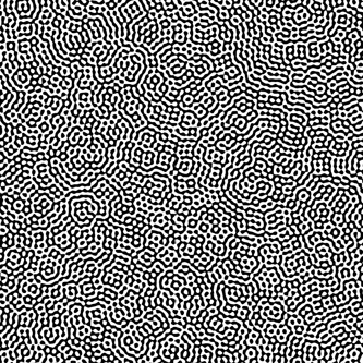
Now, to the mathematics. In two Euclidean dimensions, the random superposition of plane waves on a region $\mathcal{D}\subset\mathbb{R}^{2}$ may be written as

$$\psi_{\textsl{{n}}}(\mathbf{r})=\sqrt{\frac{2}{\mathrm{vol}\,(\mathcal{D})\,N}}\sum_{i=1}^{N}\,a_{i}\,\cos(\mathbf{k}_{i}.\mathbf{r}+\phi_{i})$$

(56)

where $a_{i}\in\mathbb{R}$ are independent Gaussian random variables with zero mean and unit variance, $\phi_{i}$ are uniformly-distributed random variables on $[0,2\pi)$, and the momenta $\mathbf{k}_{i}\in\mathbb{R}^{2}$ are randomly equidistributed, lying on the circle of radius $\sqrt{E}$. Note that the factor of $1/\sqrt{N}$ up front takes care of the normalization in the limit $N\rightarrow\infty$. A property of random waves of this type is the universality of the spatial autocorrelation function

	$\displaystyle C(\mathbf{r},\delta\mathbf{r})$	$\displaystyle=\langle\psi_{\textsc{rwm}}(\mathbf{r}-\delta\mathbf{r}/2)\,\psi_{\textsc{rwm}}(\mathbf{r}+\delta\mathbf{r}/2)\rangle$
		$\displaystyle=\frac{1}{\textrm{vol}\,(\mathcal{D})}\,J_{0}(\sqrt{E}\,\lvert\delta\mathbf{r}\rvert).$		(57)

One should be wary that Eq. (57) is not a consequence of the randomness but rather, of the dispersion relation $\lvert\,\mathbf{k}\,\rvert=\sqrt{E}$, and more directly, of the quantum ergodicity theorem. Although semiclassical techniques cannot be directly used to calculate higher-order correlations, Berry went on to conjecture that all the statistical properties of the spatial fluctuations of the eigenfunctions of a chaotic systems are described by a superposition of waves with fixed wavenumber and random phases. This description is reminiscent of the ergodicity hypothesis in statistical physics in its assertion that the spatial average in Eq. (57) is essentially equivalent to averaging over the random phases of Eq. (56). Such universal spatial fluctuations have also been identified in systems with nontrivial spin dynamics such a confined two-dimensional electron gas in the presence of spin-orbit interaction [578].

More rigorously, any wavefunction of a two-dimensional billiard obeying the Helmholtz equation with energy $E=\mathbf{k}^{2}$ can be written as the superposition (upto normalization)

$$\psi\,(r,\theta)=\sum_{n\,\in\,\mathbb{Z}}C_{n}\,J_{\lvert n\rvert}(r,\theta)\,\mathrm{e}^{\mathrm{i}\,n\,\theta},$$

(58)

where $J_{n}$ are Bessel functions and the coefficients satisfy $C_{n}=C^{*}_{-n}$ if the wavefunction is real. Berry’s conjecture contends that in the semiclassical limit $k\rightarrow\infty$, for all statistical purposes, the coefficients $C_{n}$ could be taken as independent Gaussian random variables with $\langle C_{n}\rangle=0$ and $\langle C_{n}\,C_{m}^{*}\rangle=\sigma^{2}\,\delta_{m,n}$. However, perhaps the most general way to think about a random plane wave would be to regard it as the 2D Fourier transform of white noise¹¹¹¹ 11 We use the term in the generic sense of a random signal that has equal intensity at all frequencies and thus, a flat power spectrum. on the unit circle. In this context, let $L_{\textrm{sym}}^{2}(\mathbb{T})$ denote the Hilbert space of square-integrable ($L^{2}$) functions on the unit circle with the symmetry $f(-z)=f^{*}(z)$. The Fourier image of the space $L_{\textrm{sym}}^{2}$ is simply the space of real analytic functions, $\mathcal{H}$, satisfying the Helmholtz equation. A random plane wave is then $F=\sum_{n}C_{n}\Phi_{n}$ where the $C_{n}$ are independent Gaussians and $\{\Phi_{n}\}$ is any orthonormal basis in $\mathcal{H}$; this has a covariance function $\mathrm{Cov}\,\{F(x),F(y)\}=J_{0}(\lvert x-y\rvert)$. It may seem a bit pompous to replace the simple sums over exponentials and Bessel functions with a Gaussian field in its full glory but this is, in many ways, the more natural representation to use since the first two definitions can always be extracted from it. The raison d’être for this excursion into overtly mathematical terrain is that it enables us to link our discussion to the Gaussian spherical harmonics (Fig. 14) and tap into the treasure trove of already well-known results [607] on nodal sets thereof. The connection is simple: the Gaussian plane wave is a large $n$ limit of the Gaussian spherical harmonic of degree $n$.

To be precise, consider the eigenfunctions of the Laplacian $\Delta$ on the $m$-dimensional unit sphere $\mathbb{S}^{m}$. Given an eigenvalue $E_{n}\,(n=1,2,\ldots)$, the corresponding eigenspace is the space $\mathcal{H}_{n}$ of the spherical harmonics of degree $n$, which form a $2n+1$ dimensional space of eigenfunctions of the Laplacian on $\mathbb{S}^{m}$; let $g_{n}\in\mathcal{H}_{n}$. Using integral formulae due to Poincaré and Kac-Rice (see, for example, Cramér and Leadbetter [180]), it is possible to obtain some universal estimates such as the following:

• •

  For each $g_{n}$, every nodal domain of $g_{n}$ contains a disk of radius $c\,n^{-1}$, where $c$ is an absolute constant; this tells us about the minimum size of a domain.

• •

  Let $\mathcal{Z}(g_{n})$ be the ‘volume’ of the nodal set (in two dimensions, the total length of the nodal lines). Yau [618], Yau [619] conjectured that for any smooth metric on a manifold $\mathcal{M}$, there exist constants $c\,(\mathcal{M})$, $\mathcal{C}(\mathcal{M})$ such that for every $g_{n}$, $c\,\sqrt{E_{n}}<\mathcal{Z}(g_{n})<\mathcal{C}\,\sqrt{E_{n}}$; the upper bound was also proposed by Cheng [168]. The lower bound has been proved for the planar case [144, 143] and for smooth metrics [398, 397]. We refer to [504] and [399] for estimates of the constants $c$ and $\mathcal{C}$, respectively. Although Donnelly and Fefferman [198] proved Yau’s conjecture for real-analytic metrics, the problem, in its full generality, still remains open.

• •

  For Gaussian spherical harmonics $g_{n}$, the expectation value $\mathbb{E}\,\left[\mathcal{Z}(g_{n})\right]=\pi\sqrt{2E_{n}}=\sqrt{2}\pi\,n+\mathcal{O}(1)$ [80, 626]. Subsequently, it was proved [608, 609] that

  $$\mathrm{Var}\,\mathcal{Z}(g_{n})=\frac{1}{32}\log n+\mathcal{O}(1),$$

  (59)

  which is much smaller than the prior $\mathcal{O}\,(n)$ estimate [607] on account of Berry’s cancellation phenomenon [101].

• •

  By Courant’s nodal domain theorem, and Pleijel’s refinement, $\nu\,(g_{n})<0.69\,n^{2}$. Since there are spherical harmonics with one or two nodal domains, there is no nontrivial deterministic lower bound [389]. A sharp upper bound for the number of nodal domains of spherical harmonics, for the first six eigenvalues, is given by [390]. On the other side of the coin, it is still an open problem whether—for a general surface (or higher-dimensional Riemannian manifold)—there exists a sequence of eigenfunctions for which the number of nodal domains tends to infinity with the eigenvalue. This question was answered in the affirmative for nodal domains of Maass forms [244, 245] and non-positively curved surfaces with concave boundaries, i.e., generalized Sinai or Lorentz billiards [321].

Specializing to two dimensions, $m=2$, we can exploit all of the above results on $\mathbb{S}^{2}$ for billiards.

References

- [1] Åberg, S., T. Guhr, M. Miski-Oglu, and A. Richter (2008), Phys. Rev. Lett. 100 (20), 204101.
- [2] Agam, O., and N. Brenner (1995), J. Phys. A: Math. Gen. 28 (5), 1345.
- [3] Agam, O., and S. Fishman (1993), J. Phys. A: Math. Gen. 26 (9), 2113.
- [4] Agam, O., and S. Fishman (1994), Phys. Rev. Lett. 73 (6), 806.
- [5] Ahlfors, L. V. (2010), Conformal invariants: topics in geometric function theory, Vol. 371 (American Mathematical Soc., Providence, RI).
- [6] Alberts, T. (2008), “An Introduction to the Schramm-Loewner Evolution,” Presentation (Courant Institute of Mathematical Sciences).
- [7] Aleiner, I. L., P. W. Brouwer, and L. I. Glazman (2002), Phys. Rep. 358 (5), 309.
- [8] Alessandrini, G. (1994), Comment. Math. Helv. 69 (1), 142.
- [9] Alessandrini, G. (1998), in Forum Math., Vol. 10, pp. 521–532.
- [10] Alhassid, Y. (2000), Rev. Mod. Phys. 72 (4), 895.
- [11] Alhassid, Y., and C. H. Lewenkopf (1997), Phys. Rev. B 55 (12), 7749.
- [12] Allen, L., M. W. Beijersbergen, R. J. C. Spreeuw, and J. P. Woerdman (1992), Phys. Rev. A 45 (11), 8185.
- [13] Allen, L., M. J. Padgett, and M. Babiker (1999), Prog. Opt. 39, 291.
- [14] Alt, H., C. Dembowski, H.-D. Gräf, R. Hofferbert, H. Rehfeld, A. Richter, R. Schuhmann, and T. Weiland (1997), Phys. Rev. Lett. 79 (6), 1026.
- [15] Alt, H., H.-D. Gräf, H. L. Harney, R. Hofferbert, H. Lengeler, A. Richter, P. Schardt, and H. A. Weidenmüller (1995), Phys. Rev. Lett. 74 (1), 62.
- [16] Alt, H., H.-D. Gräf, R. Hofferbert, C. Rangacharyulu, H. Rehfeld, A. Richter, P. Schardt, and A. Wirzba (1996), Phys. Rev. E 54 (3), 2303.
- [17] Anantharaman, N. (2008), Ann. Math. 168, 435.
- [18] Anantharaman, N., and S. Nonnenmacher (2007), Ann. Inst. Fourier, Grenoble 57 (7), 2465.
- [19] Ancona, A., B. Helffer, and T. Hoffmann-Ostenhof (2004), Documenta Math. 9, 283.
- [20] Andersen, M. F., A. Kaplan, T. Grünzweig, and N. Davidson (2006), Phys. Rev. Lett. 97 (10), 104102.
- [21] Andrews, B., and J. Clutterbuck (2011), J. Amer. Math. Soc. 24 (3), 899.
- [22] Antunes, P., and P. Freitas (2006), Exper. Math. 15 (3), 333.
- [23] Arendt, W., R. Nittka, W. Peter, and F. Steiner (2009), “Weyl’s law: Spectral properties of the Laplacian in mathematics and physics,” in Mathematical Analysis of Evolution, Information, and Complexity, edited by W. Arendt and W. P. Schleich (Wiley-VCH Verlag GmbH & Co., Weinheim) pp. 1–71.
- [24] Arnold, V. I. (1963), Russ. Math. Surv. 18 (5), 9.
- [25] Arnold, V. I. (1973), Uspekhi Mat. Nauk 28 (5), 260.
- [26] Arnold, V. I. (2011), Proc. Steklov Inst. Math. 273 (1), 25.
- [27] Arnold, V. I. (2013), Mathematical Methods of Classical Mechanics, 2nd ed., Vol. 60 (Springer, New York).
- [28] Arnold, V. I., and A. Avez (1967), Theorie ergodique des systemes dynamiques (Gauthier-Villars, Paris).
- [29] Aronovitch, A., R. Band, D. Fajman, and S. Gnutzmann (2012), J. Phys. A: Math. Theor. 45 (8), 085209.
- [30] Aronovitch, A., and U. Smilansky (2006), “Nodal intersections with a test curve,” Presentation (Weizmann Institute of Science).
- [31] Aronovitch, A., and U. Smilansky (2007), J. Phys. A: Math. Theor. 40 (32), 9743.
- [32] Ash, R. B., and C. Doléans-Dade (2000), Probability and measure theory, 2nd ed. (Academic Press, San Diego).
- [33] Ashbaugh, M. S. (1999), in Spectral Theory and Geometry, London Math. Soc. Lecture Note Ser., edited by E. B. Davies and Y. Safarov (Cambridge University Press, Cambridge, UK) pp. 95–139.
- [34] Ashbaugh, M. S., and R. D. Benguria (1991), Bull. Amer. Math. Soc. 25 (1), 19.
- [35] Ashbaugh, M. S., and R. D. Benguria (1992), Ann. Math. 135 (3), 601.
- [36] Ashbaugh, M. S., and R. D. Benguria (1993a), SIAM J. Math. Anal. 24 (6), 1622.
- [37] Ashbaugh, M. S., and R. D. Benguria (1993b), SIAM J. Math. Anal. 24 (3), 557.
- [38] Ashbaugh, M. S., and R. D. Benguria (2007), “Isoperimetric inequalities for eigenvalues of the laplacian,” in Spectral Theory and Mathematical Physics, Proc. Symp. Pure Math., Vol. 76 (AMS, Providence, RI) pp. 105–139.
- [39] Auberson, G., S. R. Jain, and A. Khare (2001), J. Phys. A: Math. Gen. 34 (4), 695.
- [40] Auerhammer, J., H. Genz, H.-D. Gräf, R. Hahn, P. Hoffmann-Stascheck, C. Lüttge, U. Nething, K. Rühl, A. Richter, and T. Rietdorf (1993), Nucl. Phys. A 553, 841.
- [41] Aurich, R., and F. Steiner (1988), Physica D 32 (3), 451.
- [42] Aurich, R., and F. Steiner (1993), Physica D 64 (1), 185.
- [43] Bäcker, A. (2007a), Eigenfunctions in chaotic quantum systems, Ph.D. thesis (Technische Universität Dresden).
- [44] Bäcker, A. (2007b), Eur. Phys. J. Spec. Top 145 (1), 161.
- [45] Bäcker, A., S. Fürstberger, R. Schubert, and F. Steiner (2002), J. Phys. A: Math. Gen. 35 (48), 10293.
- [46] Bäcker, A., R. Ketzmerick, and A. G. Monastra (2005), Phys. Rev. Lett. 94 (5), 054102.
- [47] Bäcker, A., and R. Schubert (2002), J Phys. A: Math. Gen. 35 (3), 527.
- [48] Bäcker, A., R. Schubert, and P. Stifter (1998a), Phys. Rev. E 58, 5192.
- [49] Bäcker, A., R. Schubert, and P. Stifter (1998b), Phys. Rev. E 57 (5), 5425.
- [50] Balian, R., and C. Bloch (1970), Ann. Phys. 60 (2), 401.
- [51] Balian, R., and C. Bloch (1971), Ann. Phys. 64 (1), 271.
- [52] Baltes, H. P., and E. R. Hilf (1976), Spectra of finite systems (BI-Wissenschaftsverlag, Mannheim).
- [53] Band, R. (2014), Phil. Trans. R. Soc. A 372 (2007), 20120504.
- [54] Band, R., I. Oren, and U. Smilansky (2008), in Analysis on Graphs and Its Applications, Proc. Symp. Pure Math., Vol. 77, edited by P. Exner, J. P. Keating, P. Kuchment, T. Sunada, and A. Teplyaev (American Mathematical Soc., Providence, RI) Chap. 1, pp. 5–27.
- [55] Band, R., O. Parzanchevski, and G. Ben-Shach (2009), J. Phys. A: Math. Theor. 42 (17), 175202.
- [56] Band, R., T. Shapira, and U. Smilansky (2006), J. Phys. A: Math. Gen. 39 (45), 13999.
- [57] Bandle, C. (1980), Isoperimetric Inequalities and Applications, Vol. 7 (Pitman Publishing, London).
- [58] Bañuelos, R., and T. Carroll (1994), Duke Math. J. 75 (3), 575.
- [59] Baranger, H. U., and P. A. Mello (1994), Phys. Rev. Lett. 73 (1), 142.
- [60] Baranova, N. B., B. Y. Zel’Dovich, A. V. Mamaev, N. Pilipetskii, and V. V. Shkukov (1981), JETP Lett. 33 (4), 206.
- [61] Barta, J. (1937), C. R. Acad. Sci. Paris 204 (7), 472.
- [62] Barth, M., and H.-J. Stöckmann (2002), Phys. Rev. E 65 (6), 066208.
- [63] Bauch, Sz., A. Błȩdowski, L. Sirko, P. M. Koch, and R. Blümel (1998), Phys. Rev. E 57 (1), 304.
- [64] Bauer, M., and D. Bernard (2002), Phys. Lett. B 543 (1), 135.
- [65] Bauer, M., and D. Bernard (2003), Commun. Math. Phys. 239 (3), 493.
- [66] Bauer, M., D. Bernard, and J. Houdayer (2005), J. Stat. Mech. 2005 (03), P03001.
- [67] Bauer, R. O. (2003), Ann. Fac. Sci. Toulouse Math. (6) 12 (4), 433.
- [68] Baxter, R. J. (2007), Exactly solved models in statistical mechanics (Dover Publications, Mineola, New York).
- [69] Bayfield, J. E., and P. M. Koch (1974), Phys. Rev. Lett. 33 (5), 258.
- [70] Beenakker, C. W. J. (1991), Phys. Rev. B 44 (4), 1646.
- [71] Beenakker, C. W. J. (1997), Rev. Mod. Phys. 69 (3), 731.
- [72] Beffara, V. (2004), Ann. Probab. 32, 2606.
- [73] Beffara, V. (2008), Ann. Probab. 36, 1421.
- [74] Beijersbergen, M. (1996), Phase singularities in optical beams, Ph.D. thesis (Huygens Laboratory, Universiteit Leiden).
- [75] Belavin, A. A., A. M. Polyakov, and A. B. Zamolodchikov (1984a), Nucl. Phys. B 241 (2), 333.
- [76] Belavin, A. A., A. M. Polyakov, and A. B. Zamolodchikov (1984b), J. Stat. Phys. 34 (5-6), 763.
- [77] Beliaev, D., and Z. Kereta (2013), J. Phys. A: Math. Theor. 46 (45), 455003.
- [78] Beliaev, D., and I. Wigman (2016), “Volume distribution of nodal domains of random band-limited functions,” arXiv preprint 1606.05766.
- [79] Benguria, R. D. (2011), “Isoperimetric Inequalities for Eigenvalues of the Laplacian,” in Entropy and the Quantum II, Contemporary Mathematics, Vol. 552, edited by R. Sims and D. Ueltschi, pp. 21–60.
- [80] Bérard, P. (1984–1985), “Volume des ensembles nodaux des fonctions propres du laplacien,” Bony-Sjoestrand-Meyer seminar, Exp. No. 14.
- [81] Bérard, P. (1992), Math. Ann. 292 (1), 547.
- [82] Bérard, P., and B. Helffer (2015), “Dirichlet eigenfunctions of the square membrane: Courant’s property, and a. stern’s and å. pleijel’s analyses,” in Analysis and Geometry: MIMS-GGTM, Tunis, Tunisia, March 2014. In Honour of Mohammed Salah Baouendi, edited by A. Baklouti, A. El Kacimi, S. Kallel, and N. Mir (Springer, Cham) pp. 69–114.
- [83] Bérard, P., and D. Meyer (1982), Ann. scient. Éc. Norm. Sup. 15 (3), 513.
- [84] Van den Berg, M., and S. Srisatkunarajah (1988), J. London Math. Soc. 37 (1), 119.
- [85] Berggren, K.-F., K. N. Pichugin, A. F. Sadreev, and A. Starikov (1999), JETP Lett. 70 (6), 403.
- [86] Berggren, K.-F., A. F. Sadreev, and A. A. Starikov (2002), Phys. Rev. E 66 (1), 016218.
- [87] Berk, N. F. (1987), Phys. Rev. Lett. 58 (25), 2718.
- [88] Bernard, D., G. Boffetta, A. Celani, and G. Falkovich (2006), Nat. Phys. 2 (2), 124.
- [89] Bernstein, D. L. (1950), Existence Theorems in Partial Differential Equations, Annals of Mathematics Studies, Vol. 23 (Princeton University Press, Princeton, NJ).
- [90] Berry, M. J., J. A. Katine, R. M. Westervelt, and A. C. Gossard (1994), Phys. Rev. B 50 (23), 17721.
- [91] Berry, M. V. (1977), J. Phys. A: Math. Gen. 10 (12), 2083.
- [92] Berry, M. V. (1978), J. Phys. A: Math. Gen. 11 (1), 27.
- [93] Berry, M. V. (1979), “Distribution of modes in fractal resonators,” in Structural Stability in Physics, edited by W. Güttinger and H. Eikemeier (Springer, Berlin, Heidelberg) pp. 51–53.
- [94] Berry, M. V. (1980), Geometry of the Laplace operator, Proc. Symp. Pure Math, 36, 13.
- [95] Berry, M. V. (1981a), Eur. J. Phys. 2 (2), 91.
- [96] Berry, M. V. (1981b), in Physics of Defects, Les Houches Lecture Series Session XXXV, Vol. 35, edited by R. Balian, M. Kléman, and J.-P. Poirier (Elsevier, North-Holland, Amsterdam) pp. 453–543.
- [97] Berry, M. V. (1983), in Chaotic Behaviour of Deterministic Systems, Les Houches Lecture Series Session XXXVI, Vol. 36, edited by G. Iooss, R. H. G. Helleman, and S. R (North-Holland Amsterdam) pp. 171–271.
- [98] Berry, M. V. (1989), Proc. R. Soc. Lond. A 423 (1864), 219.
- [99] Berry, M. V. (1991), in Chaos and Quantum Physics, Les Houches Lecture Series LII (1989), edited by M. J. Giannoni, A. Voros, and J. Zinn-Justin (Elsevier, North-Holland, Amsterdam) pp. 251–305.
- [100] Berry, M. V. (1998), in Proc. SPIE 3487, International Conference on Singular Optics, edited by M. S. Soskin, p. 1.
- [101] Berry, M. V. (2002), J. Phys. A: Math. Gen. 35 (13), 3025.
- [102] Berry, M. V., and M. R. Dennis (2000), Proc. R. Soc. Lond. A 456 (2001), 2059.
- [103] Berry, M. V., and H. Ishio (2002), J. Phys. A: Math. Gen. 35 (29), 5961.
- [104] Berry, M. V., and M. Robnik (1984), J. Phys. A: Math. Gen. 17 (12), 2413.
- [105] Berry, M. V., and M. Robnik (1986), J. Phys. A: Math. Gen. 19 (8), 1365.
- [106] Berry, M. V., and M. Tabor (1976), Proc. R. Soc. Lond. A 349 (1656), 101.
- [107] Berry, M. V., and M. Tabor (1977a), J. Phys. A: Math. Gen. 10 (3), 371.
- [108] Berry, M. V., and M. Tabor (1977b), Proc. R. Soc. Lond. A 356 (1686), 375.
- [109] Bers, L. (1955), Comm. Pure and Appl. Math. 8 (4), 473.
- [110] Bieberbach, L. (1916), Preuss. Akad. Wiss. Sitzungsb. 138, 940.
- [111] Bies, W. E., and E. J. Heller (2002), J. Phys. A: Math. Gen. 35 (27), 5673.
- [112] Bies, W. E., N. Lepore, and E. J. Heller (2003), J. Phys. A: Math. Gen. 36 (6), 1605.
- [113] Binney, J. J., N. J. Dowrick, A. J. Fisher, and M. Newman (1992), The Theory of Critical Phenomena: An Introduction to the Renormalization Group (Oxford University Press, New York).
- [114] Birkhoff, G., and G. Fix (1970), in Numerical Solution of Field Problems in Continuum Physics, SIAM-AMS Proceedings, Vol. 2, edited by G. Birkhoff and R. S. Varga (AMS, Providence, RI) pp. 111–151.
- [115] Biswas, D., and S. R. Jain (1990), Phys. Rev. A 42 (6), 3170.
- [116] Blanter, Ya. M., A. D. Mirlin, and B. A. Muzykantskii (1998), Phys. Rev. Lett. 80 (19), 4161.
- [117] Blatt, J. M., and V. F. Weisskopf (1979), Theoretical nuclear physics (Springer, New York).
- [118] Bleher, P. (1994), Duke Math. J. 74 (1), 45.
- [119] Bliokh, K. Y., I. P. Ivanov, G. Guzzinati, L. Clark, R. Van Boxem, A. Béché, R. Juchtmans, M. A. Alonso, P. Schattschneider, F. Nori, and J. Verbeek (2017), “Theory and applications of free-electron vortex states,” arXiv preprint 1703.06879.
- [120] Blum, G., S. Gnutzmann, and U. Smilansky (2002), Phys. Rev. Lett. 88, 114101.
- [121] Blümel, R., I. H. Davidson, W. P. Reinhardt, H. Lin, and M. Sharnoff (1992), Phys. Rev. A 45 (4), 2641.
- [122] Blümel, R., P. M. Koch, and L. Sirko (2001), Found. Phys. 31 (2), 269.
- [123] Bôcher, M. (1898), Bull. Amer. Math. Soc. 4 (7), 295.
- [124] Bogomolny, E. B. (1988), Physica D 31 (2), 169.
- [125] Bogomolny, E. B., O. Bohigas, and P. Leboeuf (1996), J. Stat. Phys. 85 (5-6), 639.
- [126] Bogomolny, E. B., B. Dietz, T. Friedrich, M. Miski-Oglu, A. Richter, F. Schäfer, and C. Schmit (2006a), Phys. Rev. Lett. 97 (25), 254102.
- [127] Bogomolny, E. B., R. Dubertrand, and C. Schmit (2006b), J. Phys. A: Math. Theor. 40 (3), 381.
- [128] Bogomolny, E. B., B. Georgeot, M.-J. Giannoni, and C. Schmit (1992), Phys. Rev. Lett. 69 (10), 1477.
- [129] Bogomolny, E. B., U. Gerland, and C. Schmit (1999), Phys. Rev. E 59 (2), R1315.
- [130] Bogomolny, E. B., and C. Schmit (2002), Phys. Rev. Lett. 88 (11), 114102.
- [131] Bogomolny, E. B., and C. Schmit (2004), Phys. Rev. Lett. 92 (24), 244102.
- [132] Bogomolny, E. B., and C. Schmit (2007), J. Phys. A: Math. Theor. 40 (47), 14033.
- [133] Bohigas, O., M.-J. Giannoni, and C. Schmit (1984), Phys. Rev. Lett. 52 (1), 1.
- [134] Bohr, A., and B. R. Mottelson (1998), Nuclear structure, Vol. 1 (World Scientific, Singapore).
- [135] Bolte, J. (1993), Int. J. Mod. Phys. B 7 (27), 4451.
- [136] Bolte, J., G. Steil, and F. Steiner (1992), Phys. Rev. Lett. 69 (15), 2188.
- [137] Borell, C. (1975), Invent. Math. 30 (2), 207.
- [138] Borgonovi, F. (1998), Phys. Rev. Lett. 80 (21), 4653.
- [139] Brack, M. (1993), Rev. Mod. Phys. 65 (3), 677.
- [140] Brack, M., and R. K. Bhaduri (2003), Semiclassical physics, Vol. 96 (Westview Press, Boulder, CO).
- [141] Brink, D. M., and R. O. Stephen (1963), Phys. Lett. 5 (1), 77.
- [142] Brossard, J., and R. Carmona (1986), Commun. Math. Phys. 104 (1), 103.
- [143] Brüning, J. (1978), Math. Z. 158 (1), 15.
- [144] Brüning, J., and D. Gromes (1972), Math. Z. 124 (1), 79.
- [145] Buckley, J., and I. Wigman (2016), Ann. Henri Poincaré 17 (11), 3027.
- [146] Bunimovich, L. A. (2001), Chaos 11 (4), 802.
- [147] Bunimovich, L. A. (2007), Scholarpedia 2 (8), 1813.
- [148] Bunimovich, L. A., D. Burago, N. Chernov, E. G. D. Cohen, C. P. Dettmann, J. R. Dorfman, S. Ferleger, R. Hirschl, A. Kononenko, J. L. Lebowitz, C. Liverani, T. J. Murphy, J. Piasecki, H. A. Posch, N. Simanyi, Ya. G. Sinaĭ, T. Tel, H. van Beijeren, R. van Zon, J. Vollmer, and L. S. Young (2013), Hard Ball Systems and the Lorentz Gas, edited by D. Szász, Encylopaedia of Mathematical Sciences, Vol. 101 (Springer, Heidelberg).
- [149] Bunimovich, L. A., and Ya. G. Sinaĭ (1981), Commun. Math. Phys. 78 (4), 479.
- [150] Burenkov, V. I., and E. B. Davies (2002), J. Differential Equations 186 (2), 485.
- [151] Buser, P., J. Conway, P. Doyle, and K.-D. Semmler (1994), Int. Math. Res. Not. 1994 (9), 391.
- [152] Canzani, Y., and P. Sarnak (2014), “On the topology of the zero sets of monochromatic random waves,” arXiv preprint 1412.4437.
- [153] Canzani, Y., and P. Sarnak (2016), “Topology and nesting of the zero set components of monochromatic random waves,” arXiv preprint 1701.00034.
- [154] Cardy, J. L. (1984), Nucl. Phys. B 240 (4), 514.
- [155] Cardy, J. L. (1992), J. Phys. A: Math. Gen. 25 (4), L201.
- [156] Cardy, J. L. (2003), J. Phys. A: Math. Gen. 36 (24), L379.
- [157] Cardy, J. L. (2005), Ann. Phys. 318 (1), 81.
- [158] Cardy, J. L. (2006), Nat. Phys. 2 (2), 67.
- [159] Casati, G., and J. Ford (1979), Stochastic Behavior in Classical and Quantum Hamiltonian systems, Lecture Notes in Physics, Vol. 93 (Springer, Berlin).
- [160] Chang, P.-K., and D. DeTurck (1989), Proc. Amer. Math. Soc. 105 (4), 1033.
- [161] Chapman, S. J. (1995), Amer. Math. Monthly 102 (2), 124.
- [162] Chavel, I. (1984), Eigenvalues in Riemannian geometry, Vol. 115 (Academic Press, Orlando, FL).
- [163] Chen, Y. F., and K. F. Huang (2003a), Phys. Rev. E 68 (6), 066207.
- [164] Chen, Y. F., and K. F. Huang (2003b), J. Phys. A: Math. Gen. 36 (28), 7751.
- [165] Chen, Y. F., K. F. Huang, and Y. P. Lan (2002), Phys. Rev. E 66 (6), 066210.
- [166] Chen, Y. F., Y. C. Lin, W. Z. Zhuang, H. C. Liang, K. W. Su, and K. F. Huang (2012), Phys. Rev. A 85 (4), 043833.
- [167] Chen, Y. F., K. W. Su, T.-H. Lu, and K. F. Huang (2006), Phys. Rev. Lett. 96 (3), 033905.
- [168] Cheng, S.-Y. (1976), Comment. Math. Helv. 51 (1), 43.
- [169] Chibotaru, L. F., A. Ceulemans, V. Bruyndoncx, and V. V. Moshchalkov (2001), Phys. Rev. Lett. 86 (7), 1323.
- [170] Chladni, E. F. F. (1787), Entdeckungen über die Theorie des Klanges (Zentralantiquariat der DDR, Leipzig).
- [171] Chladni, E. F. F. (1802), Die Akustik (Breitkopf und Härtel, Leipzig).
- [172] Cipra, B. (1992), Science 255 (5052), 1642.
- [173] Coffman, C. V. (1982), SIAM J. Math. Anal. 13 (5), 746.
- [174] Coffman, C. V., and R. J. Duffin (1980), Adv. Appl. Math. 1 (4), 373.
- [175] Collin, R. E. (1960), Field theory of guided waves (McGraw-Hill, New York).
- [176] Couchman, L., E. Ott, and T. M. Antonsen Jr. (1992), Phys. Rev. A 46 (10), 6193.
- [177] Courant, R. (1923), Nachr. Ges. Wiss. Göttingen, Math.-Phys. Kl. 1, 81.
- [178] Courant, R., and D. Hilbert (1953), Methods of Mathematical Physics, Vol. 1 (Interscience Publishers Inc., New York).
- [179] Courtial, J., and K. O’Holleran (2007), Eur. Phys. J. Spec. Top. 145 (1), 35.
- [180] Cramér, H., and M. R. Leadbetter (2013), Stationary and related stochastic processes: Sample function properties and their applications (Dover Publications, Mineola, New York).
- [181] Cuesta, M., D. G. De Figueiredo, and J.-P. Gossez (2000), C. R. Acad. Sci. Paris Sér. I Math. 330 (8), 669.
- [182] Davies, E. B. (1996), Spectral theory and differential operators, Vol. 42 (Cambridge University Press, Cambridge, UK).
- [183] De Branges, L. (1985), Acta Math. 154 (1), 137.
- [184] DeMarco, L. (2011), Bull. Amer. Math. Soc. 48 (1), 33.
- [185] Dembowski, C., B. Dietz, H.-D. Gräf, A. Heine, F. Leyvraz, M. Miski-Oglu, A. Richter, and T. H. Seligman (2003), Phys. Rev. Lett. 90 (1), 014102.
- [186] Dembowski, C., H.-D. Gräf, A. Heine, R. Hofferbert, H. Rehfeld, and A. Richter (2000), Phys. Rev. Lett. 84 (5), 867.
- [187] Dennis, M. R. (2001), J. Phys. A: Math. Gen. 34 (20), L297.
- [188] Dennis, M. R. (2003), J. Phys. A: Math. Gen. 36 (24), 6611.
- [189] Dennis, M. R., K. O’Holleran, and M. J. Padgett (2009), Prog. Opt. 53, 293.
- [190] Desjardins, S. (1998), Differential Geom. Appl. 8 (3), 257.
- [191] Desjardins, S., and P. Gilkey (1994), Mathematische Z. 215 (1), 251.
- [192] Deus, S., P. M. Koch, and L. Sirko (1995), Phys. Rev. E 52 (1), 1146.
- [193] Dietz, B., T. Friedrich, M. Miski-Oglu, A. Richter, and F. Schäfer (2008), Phys. Rev. E 78 (4), 045201.
- [194] Dietz, B., A. Heusler, K. H. Maier, A. Richter, and B. A. Brown (2017), Phys. Rev. Lett. 118 (1), 012501.
- [195] Dietz, B., A. Richter, and R. Samajdar (2015), Phys. Rev. E 92 (2), 022904.
- [196] Dirac, P. A. M. (1931), Proc. R. Soc. Lond. A 133, 60.
- [197] Donnelly, H. (2011), Math. Z. 269 (1), 1.
- [198] Donnelly, H., and C. Fefferman (1988), Invent. Math. 93 (1), 161.
- [199] Donnelly, H., and C. Fefferman (1990), “Nodal sets of eigenfunctions: Riemannian manifolds with boundary,” in Analysis, et Cetera (Academic Press, Boston, MA) pp. 251–262.
- [200] Doron, E., and U. Smilansky (1992a), Phys. Rev. Lett. 68 (9), 1255.
- [201] Doron, E., and U. Smilansky (1992b), Nonlinearity 5 (5), 1055.
- [202] Doron, E., U. Smilansky, and A. Frenkel (1990), Phys. Rev. Lett. 65 (25), 3072.
- [203] Drábek, P., and S. B. Robinson (2002), J. Differential Equations 181 (1), 58.
- [204] Duffin, R. J. (1948), J. Math. & Phys. [Stud. Appl. Math.] 27 (1-4), 253.
- [205] Duplantier, B. (2000), Phys. Rev. Lett. 84 (7), 1363.
- [206] Durvasula, S. (1968), J. Acoust. Soc. Am 44 (6), 1636.
- [207] Eckhardt, B., J. Ford, and F. Vivaldi (1984), Physica D 13 (3), 339.
- [208] Edmunds, D. E., and W. D. Evans (1987), Spectral theory and differential operators, Oxford Mathematical Monographs, Vol. 15 (Oxford University Press, Oxford, UK).
- [209] Ellegaard, C., T. Guhr, K. Lindemann, H. Q. Lorensen, J. Nygård, and M. Oxborrow (1995), Phys. Rev. Lett. 75 (8), 1546.
- [210] Elon, Y., S. Gnutzmann, C. Joas, and U. Smilansky (2007), J. Phys. A: Math. Theor. 40 (11), 2689.
- [211] Faber, G. (1923), Sitz. Bayer. Akad. Wiss. 8, 169.
- [212] Falkovich, G. (2007), Eur. Phys. J. Spec. Top. 145 (1), 211.
- [213] Faraday, M. (1859), Experimental researches in chemistry and physics (Taylor & Francis, London).
- [214] Feder, J. (1988), Fractals, Physics of Solids and Liquids (Springer, New York).
- [215] Fisher, M. E. (1966), J. Combin. Theory 1 (1), 105.
- [216] Fisher, M. E. (1967), Rep. Prog. Phys. 30 (2), 615.
- [217] Fishman, S., B. Georgeot, and R. E. Prange (1996), J. Phys. A: Math. Gen. 29 (4), 919.
- [218] Flores, J. (2007), Eur. Phys. J. Spec. Top. 145 (1), 63.
- [219] Fogedby, H. C. (2012), in Computational Complexity, edited by R. A. Meyers (Springer) pp. 3075–3096.
- [220] Foltin, G. (2003a), “Counting nodal domains,” arXiv preprint nlin/0302049.
- [221] Foltin, G. (2003b), J. Phys. A: Math. Gen. 36 (6), 4561.
- [222] Foltin, G. (2003c), J. Phys. A: Math. Gen. 36 (6), 1729.
- [223] Foltin, G., S. Gnutzmann, and U. Smilansky (2004a), J. Phys. A: Math. Gen. 37 (47), 11363.
- [224] Foltin, G., S. Gnutzmann, and U. Smilansky (2004b), “The morphology of nodal lines-random waves versus percolation,” arXiv preprint nlin/0407012.
- [225] Fournais, S. (2001), J. Differential Equations 173 (1), 145.
- [226] Freitas, P. (2006), Proc. Amer. Math. Soc. , 2083.
- [227] Freitas, P. (2007), J. Funct. Anal. 251 (1), 376.
- [228] Freitas, P., and D. Krejčiřik (2008), Proc. Amer. Math. Soc. 136 (8), 2997.
- [229] Freund, I. (1994), J. Opt. Soc. Am. A 11 (5), 1644.
- [230] Freund, I. (1997), J. Opt. Soc. Am. A 14 (8), 1911.
- [231] Freund, I. (1999), Opt. Commun. 159 (1), 99.
- [232] Freund, I., and V. Freilikher (1997), J. Opt. Soc. Am. A 14 (8), 1902.
- [233] Freund, I., and N. Shvartsman (1994), Phys. Rev. A 50 (6), 5164.
- [234] Freund, I., N. Shvartsman, and V. Freilikher (1993), Opt. Commun. 101 (3-4), 247.
- [235] Freund, I., and M. Wilkinson (1998), J. Opt. Soc. Am. A 15 (11), 2892.
- [236] Friedman, N., A. Kaplan, D. Carasso, and N. Davidson (2001), Phys. Rev. Lett. 86 (8), 1518.
- [237] Fyodorov, Yu. V., D. V. Savin, and H.-J. Sommers (2005), J. Phys. A: Math. Gen. 38 (49), 10731.
- [238] Garabedian, P. R. (1950), Pacific J. Math. 1 (4), 485.
- [239] Garcés-Chávez, V., D. McGloin, M. J. Padgett, W. Dultz, H. Schmitzer, and K. Dholakia (2003), Phys. Rev. Lett. 91 (9), 093602.
- [240] Gayet, D., and J.-Y. Welschinger (2014a), “Betti numbers of random nodal sets of elliptic pseudo-differential operators,” arXiv preprint 1406.0934.
- [241] Gayet, D., and J.-Y. Welschinger (2014b), J. London Math. Soc. 90 (1), 105.
- [242] Gayet, D., and J.-Y. Welschinger (2015), J. Inst. Math. Jussieu 14 (4), 673.
- [243] Gérard, P., and E. Leichtnam (1993), Duke Math. J. 71 (2), 559.
- [244] Ghosh, A., A. Reznikov, and P. Sarnak (2013), Geom. Funct. Anal. 23 (5), 1515.
- [245] Ghosh, A., A. Reznikov, and P. Sarnak (2015), “Nodal domains of maass forms ii,” arXiv preprint 1510.02963.
- [246] Giraud, O., and K. Thas (2010), Rev. Mod. Phys. 82 (3), 2213.
- [247] Girouard, A., N. Nadirashvili, and I. Polterovich (2009), J. Differential Geom. 83 (3), 637.
- [248] Glashow, S. L., and L. Mittag (1997), J. Stat. Phys. 87 (3-4), 937.
- [249] Gnutzmann, S., P. D. Karageorge, and U. Smilansky (2006), Phys. Rev. Lett. 97 (9), 090201.
- [250] Gnutzmann, S., P. D. Karageorge, and U. Smilansky (2007), Eur. Phys. J. Spec. Top. 145 (1), 217.
- [251] Gnutzmann, S., and S. Lois (2014), Phil. Trans. R. Soc. A 372 (2007), 20120521.
- [252] Gnutzmann, S., U. Smilansky, and N. Sondergaard (2005), J. Phys. A: Math. Gen. 38 (41), 8921.
- [253] Gnutzmann, S., U. Smilansky, and J. Weber (2004), Wave. Random Media 14 (1), S61.
- [254] Goldstein, S., J. L. Lebowitz, R. Tumulka, and N. Zanghi (2006), J. Stat. Phys. 125 (5-6), 1193.
- [255] Gomes, S. (2015), “Percival’s Conjecture for the Bunimovich Mushroom Billiard,” arXiv preprint 1504.07332.
- [256] Gong, S. (1999), The Bieberbach Conjecture, Studies in Advanced Mathematics, Vol. 12 (American Mathematical Soc., Providence, RI).
- [257] Goodman, J. W. (2015), Statistical Optics, 2nd ed. (John Wiley and Sons, New York).
- [258] Gordon, C., and D. Webb (1994), Math. Res. Lett 1 (5), 539.
- [259] Gordon, C., D. L. Webb, and S. Wolpert (1992a), Invent. Math. 110 (1), 1.
- [260] Gordon, C., D. L. Webb, and S. Wolpert (1992b), Bull. Amer. Math. Soc. 27 (1), 134.
- [261] Gornyi, I. V., and A. D. Mirlin (2002), Physica E 12 (1), 845.
- [262] Gough, C. (2007), Eur. Phys. J. Spec. Top. 145 (1), 77.
- [263] Gräf, H.-D., H. L. Harney, H. Lengeler, C. H. Lewenkopf, C. Rangacharyulu, A. Richter, P. Schardt, and H. A. Weidenmüller (1992), Phys. Rev. Lett. 69 (9), 1296.
- [264] Grandy Jr., W. (1987), Foundations of Statistical Mechanics: Equilibrium Theory, Vol. 1 (D. Reidel Publishing Company, Dordrecht).
- [265] Grebenkov, D. S., and B.-T. Nguyen (2013), SIAM Rev. 55 (4), 601.
- [266] Grémaud, B., and S. R. Jain (1998), J. Phys. A: Math. Gen. 31 (37), L637.
- [267] Grieser, D., and D. Jerison (1996), Invent. Math. 125 (2), 197.
- [268] Grieser, D., and S. Maronna (2013), Notices Amer. Math. Soc. 60 (11), 10.1090/noti1063.
- [269] Gruzberg, I. A., and L. P. Kadanoff (2004), J. Stat. Phys. 114 (5-6), 1183.
- [270] Gutkin, B., and U. Smilansky (2001), J. Phys. A: Math. Gen. 34 (31), 6061.
- [271] Gutzwiller, M. C. (2013), Chaos in Classical and Quantum Mechanics, Interdisciplinary Applied Mathematics, Vol. 1 (Springer, New York).
- [272] Haake, F. (2013), Quantum signatures of chaos, 2nd ed., Vol. 54 (Springer, Berlin Heidelberg).
- [273] Hale, J. K. (2005), “Eigenvalues and perturbed domains,” in Ten Mathematical Essays on Approximation in Analysis and Topology, edited by J. Ferrera, J. López-Gómez, and F. R. R. del Portal (Elsevier, Amsterdam) pp. 95–123.
- [274] Halperin, B. I. (1981), in Physics of Defects, Les Houches lecture series, Vol. 35, edited by R. Balian, M. Kléman, and J.-P. Poirier (Elsevier, North-Holland, Amsterdam) pp. 814–857.
- [275] Hannay, J. H., and M. V. Berry (1980), Physica D 1 (3), 267.
- [276] Hansen, W., and N. Nadirashvili (1994), “Isoperimetric inequalities in potential theory,” in ICPT ’91: Proceedings from the International Conference on Potential Theory, edited by E. Bertin (Springer Netherlands, Dordrecht) pp. 1–14.
- [277] Hardy, G. H., and E. M. Wright (1979), An Introduction to the Theory of Numbers, 5th ed. (Oxford University Press, London).
- [278] Harris, A. B. (1974), J. Phys. C: Solid State Phys. 7 (9), 1671.
- [279] Hayman, W. K. (1978), Appl. Anal. 7 (3), 247.
- [280] He, H., M. E. J. Friese, N. R. Heckenberg, and H. Rubinsztein-Dunlop (1995), Phys. Rev. Lett. 75 (5), 826.
- [281] Helffer, B., A. Martinez, and D. Robert (1987), Commun. Math. Phys. 109 (2), 313.
- [282] Helffer, B., and M. P. Sundqvist (2015), Mosc. Math. J 15 (3), 455.
- [283] Heller, E. J. (1984), Phys. Rev. Lett. 53 (16), 1515.
- [284] Heller, E. J., and B. Landry (2007), Eur. Phys. J. Spec. Top. 145 (1), 231.
- [285] von Helmholtz, H. (1865), Die Lehre von den Tonempfindungen als physiologische Grundlage für die Theorie der Musik (Vieweg, Braunschweig).
- [286] Hempel, R., L. A. Seco, and B. Simon (1991), J. Funct. Anal. 102 (2), 448.
- [287] Henkel, M., and D. Karevski, Eds. (2012), Conformal Invariance: An Introduction to Loops, Interfaces and Stochastic Loewner Evolution, Lecture Notes in Physics, Vol. 853 (Springer, Berlin Heidelberg).
- [288] Henrot, A. (2006), Extremum Problems for Eigenvalues of Elliptic Operators, Front. Math. (Basel: Birkhäuser Verlag).
- [289] Herrmann, H. (1932), Beiträge zur Theorie der Eigenwerte und Eigenfunktionen, Ph.D. thesis (Georg-August-Universität Göttingen).
- [290] Herrmann, H. (1936), Math. Z. 40 (1), 221.
- [291] Hersch, J. (1960), Z. Angew. Math. Phys. 11 (5), 387.
- [292] Hile, G. N., and M. H. Protter (1980), Indiana Univ. Math. J. 29 (4), 523.
- [293] Hlushchuk, Y., A. Kohler, Sz. Bauch, L. Sirko, R. Blümel, M. Barth, and H.-J. Stöckmann (2000), Phys. Rev. E 61 (1), 366.
- [294] Hoffmann-Ostenhof, M., T. Hoffmann-Ostenhof, and N. Nadirashvili (1997), Duke Math. J. 90 (3), 631.
- [295] Hoffmann-Ostenhof, M., T. Hoffmann-Ostenhof, and N. Nadirashvili (1999a), Ann. Global Anal. Geom. 17 (1), 43.
- [296] Hoffmann-Ostenhof, T., P. W. Michor, and N. Nadirashvili (1999b), Geom. Funct. Anal. 9 (6), 1169.
- [297] Höhmann, R., U. Kuhl, H.-J. Stöckmann, J. D. Urbina, and M. R. Dennis (2009), Phys. Rev. E 79 (1), 016203.
- [298] Holle, A., G. Wiebusch, J. Main, B. Hager, H. Rottke, and K. H. Welge (1986), Phys. Rev. Lett. 56 (24), 2594.
- [299] Hortikar, S., and M. Srednicki (1998), Phys. Rev. Lett. 80 (8), 1646.
- [300] Hoshen, J., and R. Kopelman (1976), Phys. Rev. B 14 (8), 3438.
- [301] Houston, A. J. H., M. Gradhand, and M. R. Dennis (2017), J. Phys. A: Math. Theor. 50 (20), 205101.
- [302] Huang, K. F., Y. F. Chen, H. C. Lai, and Y. P. Lan (2002), Phys. Rev. Lett. 89 (22), 224102.
- [303] Hul, O., S. Bauch, P. Pakoński, N. Savytskyy, K. Życzkowski, and L. Sirko (2004), Phys. Rev. E 69 (5), 056205.
- [304] Hul, O., M. Ławniczak, S. Bauch, A. Sawicki, M. Kuś, and L. Sirko (2012), Phys. Rev. Lett. 109 (4), 040402.
- [305] Hul, O., N. Savytskyy, O. Tymoshchuk, S. Bauch, and L. Sirko (2005), Phys. Rev. E 72 (6), 066212.
- [306] Ikeda, A. (1980), Ann. scient. Éc. Norm. Sup. 13 (3), 303.
- [307] Ishio, H., A. I. Saichev, A. F. Sadreev, and K.-F. Berggren (2001), Phys. Rev. E 64 (5), 056208.
- [308] Itô, K. (1944), Proc. Imp. Acad. 20 (8), 519.
- [309] Itzykson, C., and J. Luck (1986), J. Phys. A: Math. Gen. 19 (2), 211.
- [310] Ivrii, V. Ya.. (1980), Funct. Anal. Appl. 14 (2), 98.
- [311] Jackson, J. D. (1999), Classical electrodynamics, 3rd ed. (John Wiley and Sons, New York).
- [312] Jain, S. R. (2009), Pramana - J. Phys. 72 (3), 611.
- [313] Jain, S. R., B. Grémaud, and A. Khare (2002), Phys. Rev. E 66 (1), 016216.
- [314] Jakobson, D., N. Nadirashvili, and J. A. Toth (2001), Russ. Math. Surv. 56 (6), 1085.
- [315] Jalabert, R. A., J.-L. Pichard, and C. W. J. Beenakker (1994), EPL 27 (4), 255.
- [316] Jalabert, R. A., A. D. Stone, and Y. Alhassid (1992), Phys. Rev. Lett. 68 (23), 3468.
- [317] Jensen, H. C. (1955), Am. J. Phys. 23 (8), 503.
- [318] Jerison, D. (1991), Int. Math. Res. Notices 1991 (1), 1.
- [319] Jerison, D. (1995), Ann. Math. 141 (1), 1.
- [320] Johansson, K. (2002), Probab. Theory Relat. Fields 123 (2), 225.
- [321] Jung, J., and S. Zelditch (2016), Math. Ann. 364 (3-4), 813.
- [322] Kac, M. (1959), Probability and related topics in physical sciences, Vol. 1 (American Mathematical Soc., Providence, RI).
- [323] Kac, M. (1966), Amer. Math. Monthly 73 (4), 1.
- [324] Kager, W., and B. Nienhuis (2004), J. Stat. Phys. 115 (5–6), 1149.
- [325] Kager, W., B. Nienhuis, and L. P. Kadanoff (2004), J. Stat. Phys. 115 (3-4), 805.
- [326] Kaplan, L. (1999), Nonlinearity 12 (2), R1.
- [327] Kaplan, L., and E. J. Heller (1998), Ann. Phys. 264 (2), 171.
- [328] Kaplan, L., and E. J. Heller (1999), Phys. Rev. E 59 (6), 6609.
- [329] Karageorge, P. D., and U. Smilansky (2008), J. Phys. A: Math. Theor. 41 (20), 205102.
- [330] Karman, G. P., M. W. Beijersbergen, A. Van Duijl, and J. P. Woerdman (1997), Opt. Lett. 22 (19), 1503.
- [331] Keating, J. P. (1991), Nonlinearity 4 (2), 309.
- [332] Keating, J. P., J. Marklof, and I. G. Williams (2006), Phys. Rev. Lett. 97 (3), 034101.
- [333] Keating, J. P., J. Marklof, and I. G. Williams (2008), New J. Phys. 10 (8), 083023.
- [334] Keating, J. P., and S. D. Prado (2001), Proc. R. Soc. Lond. A 457 (2012), 1855.
- [335] Kelvin, L. (1901), Phil. Mag. Ser. 6 2 (7), 1.
- [336] Kennedy, J. B. (2011), J. Differential Equations 251 (12), 3606.
- [337] Kennedy, T. (2007), J. Stat. Phys. 128 (5), 1125.
- [338] Kenyon, R. (2000), Acta Math. 185, 239.
- [339] Kereta, Z. (2012), Numerical study into validity of the Bogomolny-Schmit conjecture, Master’s thesis (University of Oxford).
- [340] Kim, Y.-H., M. Barth, U. Kuhl, and H.-J. Stöckmann (2003), Prog. Theor. Phys. Supp. 150, 105.
- [341] Klawonn, D. (2009), J. Phys. A: Math. Theor. 42 (17), 175209.
- [342] Klein, A., and O. Agam (2011), J. Phys. A: Math. Theor. 45 (2), 025001.
- [343] Kollmann, M., J. Stein, U. Stoffregen, H.-J. Stöckmann, and B. Eckhardt (1994), Phys. Rev. E 49 (1), R1.
- [344] Kolmogorov, A. N. (1954), Dokl. Akad. Nauk SSSR 98 (4), 527.
- [345] Konrad, K. (2012), “Asymptotic statistics of nodal domains of quantum chaotic billiards in the semiclassical limit,” Senior thesis (Dartmouth College).
- [346] Kozlov, V. A., V. A. Kondrat’ev, and V. G. Maz’ya (1990), Math. USSR Izvestiya 34 (2), 337.
- [347] Krahn, E. (1925), Math. Ann. 94 (1), 97.
- [348] Krahn, E. (1926), Acta Comm. Univ. Tartu (Dorpat) A9, 1.
- [349] Krishnamurthy, H. R., H. S. Mani, and H. C. Verma (1982), J. Phys. A: Math. Gen. 15 (7), 2131.
- [350] Krishnapur, M., P. Kurlberg, and I. Wigman (2013), Ann. Math. 177 (2), 699.
- [351] Kröger, P. (1992), J. Funct. Anal. 106 (2), 353.
- [352] Krylov, N. S. (1979), Works on the Foundations of Statistical Physics (Princeton University Press, Princeton, NJ).
- [353] Kuchment, P. (2008), in Analysis on Graphs and Its Applications, Proc. Symp. Pure Math., Vol. 77, edited by P. Exner, J. P. Keating, P. Kuchment, T. Sunada, and A. Teplyaev (American Mathematical Soc., Providence, RI) Chap. 3, pp. 291–314.
- [354] Kudrolli, A., V. Kidambi, and S. Sridhar (1995), Phys. Rev. Lett. 75 (5), 822.
- [355] Kudrolli, A., S. Sridhar, A. Pandey, and R. Ramaswamy (1994), Phys. Rev. E 49 (1), R11.
- [356] Kuhl, U. (2007), Eur. Phys. J. Spec. Top. 145 (1), 103.
- [357] Kuhl, U., R. Höhmann, H.-J. Stöckmann, and S. Gnutzmann (2007), Phys. Rev. E 75 (3), 036204.
- [358] Kuhl, U., M. Martinez-Mares, R. A. Méndez-Sánchez, and H.-J. Stöckmann (2005a), Phys. Rev. Lett. 94 (14), 144101.
- [359] Kuhl, U., E. Persson, M. Barth, and H.-J. Stöckmann (2000), Eur. Phys. J. B 17 (2), 253.
- [360] Kuhl, U., H.-J. Stöckmann, and R. Weaver (2005b), J. Phys. A: Math. Gen. 38 (49), 10433.
- [361] Kurlberg, P., and I. Wigman (2015), C. R. Math. 353 (2), 101.
- [362] Kurlberg, P., and I. Wigman (2016), Math. Ann. 0, 1.
- [363] Kuttler, J. R., and V. G. Sigillito (1984), SIAM Rev. 26 (2), 163.
- [364] Kuznetsov, N. (2015), “On Delusive Nodes of Free Oscillations,” arXiv preprint 1502.00601.
- [365] Lai, R., Y. Shi, I. Dinov, T. F. Chan, and A. W. Toga (2009), in 2009 IEEE International Symposium on Biomedical Imaging: From Nano to Macro (IEEE) pp. 694–697.
- [366] Lai, R., Y. Shi, K. Scheibel, S. Fears, R. Woods, A. W. Toga, and T. F. Chan (2010), in 2010 IEEE Computer Society Conference on Computer Vision and Pattern Recognition (IEEE) pp. 2871–2878.
- [367] Lamé, G. (1866), Leçons sur la théorie mathématique de l’elasticité des corps solides (Gauthier-Villars, Bachelier, Paris).
- [368] Landau, E. (1909), Arch. Math. Phys. (III) 13, 305.
- [369] Landau, L. D., and E. M. Lifshitz (1959), Theory of Elasticity, Course of Theoretical Physics, Vol. 7 (Pergamon Press, Oxford).
- [370] van Langen, S. A., P. W. Brouwer, and C. W. J. Beenakker (1997), Phys. Rev. E 55 (1), R1.
- [371] Lapidus, M. L. (1991), Trans. Amer. Math. Soc. 325 (2), 465.
- [372] Lapidus, M. L., and C. Pomerance (1993), Proc. London Math. Soc. 3 (1), 41.
- [373] Lapidus, M. L., and C. Pomerance (1996), Math. Proc. Cambridge Philos. Soc. 119 (1), 167.
- [374] Lawler, G. F. (2001), in Proceedings of Conference on Random Walks (Erwin Schrödinger Institute, Vienna).
- [375] Lawler, G. F. (2008), Conformally invariant processes in the plane, Mathematical Surveys and Monographs, Vol. 114 (American Mathematical Soc., Providence, RI).
- [376] Lawler, G. F. (2009), Bull. Amer. Math. Soc. 46 (1), 35.
- [377] Lawler, G. F., O. Schramm, and W. Werner (2000), Math. Res. Lett. 8 (4), 401.
- [378] Lawler, G. F., O. Schramm, and W. Werner (2001a), Acta Math. 187, 237.
- [379] Lawler, G. F., O. Schramm, and W. Werner (2001b), Acta Math. 187, 275.
- [380] Lawler, G. F., O. Schramm, and W. Werner (2002), Ann. Inst. H. Poincaré Probab. Statist. 38, 109.
- [381] Lawler, G. F., O. Schramm, and W. Werner (2003), J. Amer. Math. Soc. 16 (4), 917.
- [382] Lawler, G. F., O. Schramm, and W. Werner (2004a), Ann. Probab. 32, 939.
- [383] Lawler, G. F., O. Schramm, and W. Werner (2004b), in Fractal Geometry and Applications: A Jubilee of Benoit Mandelbrot, Proc. Symp. Pure Math., Vol. 72.2, edited by M. L. Lapidus and M. van Frankenhuijsen (American Mathematical Soc., Providence, RI).
- [384] Ławniczak, M., A. Sawicki, S. Bauch, M. Kuś, and L. Sirko (2014), Phys. Rev. E 89 (3), 032911.
- [385] Lehmann, N., D. Saher, V. V. Sokolov, and H.-J. Sommers (1995), Nucl. Phys. A 582 (1), 223.
- [386] Levitin, M., and D. Vassiliev (1996), Proc. London Math. Soc. 3 (1), 188.
- [387] Lévy, P. (1965), Processus stochastiques et mouvement brownien (Gauthier-Villars, Paris).
- [388] Lewenkopf, C. H., A. Müller, and E. Doron (1992), Phys. Rev. A 45 (4), 2635.
- [389] Lewy, H. (1977), Commun. Part. Diff. Eq. 2 (12), 1233.
- [390] Leydold, J. (1996), Topology 35 (2), 301.
- [391] Li, B., and M. Robnik (1994), J. Phys. A: Math. Gen. 27 (16), 5509.
- [392] Liboff, R. L. (1994), J. Math. Phys. 35 (8), 3881.
- [393] Lichtenberg, A. J., and M. A. Lieberman (2013), Regular and stochastic motion, Applied Mathematical Sciences, Vol. 38 (Springer, New York).
- [394] Lin, C.-S. (1987), Commun. Math. Phys. 111 (2), 161.
- [395] Lin, C. S., and W.-M. Ni (1988), Proc. Amer. Math. Soc. 102 (2), 271.
- [396] Loewner, Ch. (1953), Pacific J. Math 3, 417.
- [397] Logunov, A. (2016a), “Nodal sets of laplace eigenfunctions: polynomial upper estimates of the hausdorff measure,” arXiv preprint 1605.02587.
- [398] Logunov, A. (2016b), “Nodal sets of laplace eigenfunctions: proof of nadirashvili’s conjecture and of the lower bound in yau’s conjecture,” arXiv preprint 1605.02589.
- [399] Logunov, A., and E. Malinnikova (2016), “Nodal sets of laplace eigenfunctions: estimates of the hausdorff measure in dimension two and three,” arXiv preprint 1605.02595.
- [400] Longuet-Higgins, M. S. (1957), Phil. Trans. R. Soc. A 249 (966), 321.
- [401] Löwner, K. (1923), Math. Ann. 89 (1), 103.
- [402] Lu, W. T., S. Sridhar, and M. Zworski (2003), Phys. Rev. Lett. 91 (15), 154101.
- [403] Lukaschuk, S., P. Denissenko, and G. Falkovich (2007), Eur. Phys. J. Spec. Top. 145 (1), 125.
- [404] Maffucci, R. W. (2016), Monatsh. Math. , 1.
- [405] Maier Jr, L. C., and J. C. Slater (1952), J. Appl. Phys. 23 (1), 68.
- [406] Main, J., G. Wiebusch, A. Holle, and K. H. Welge (1986), Phys. Rev. Lett. 57 (22), 2789.
- [407] Makai, E. (1965), Acta Math. Hung. 16 (3-4), 319.
- [408] Mandelbrot, B. B. (1983), The Fractal Geometry of Nature, Vol. 173 (Macmillan).
- [409] Mandwal, A. K., and S. R. Jain (2017), Pramana - J. Phys. 89, 35.
- [410] Mangoubi, D. (2008), Canad. Math. Bull. 51 (2), 249.
- [411] Manjunath, N., R. Samajdar, and S. R. Jain (2016), Ann. Phys. 372, 68.
- [412] Marinucci, D., G. Peccati, M. Rossi, and I. Wigman (2016), Geom. Funct. Anal. 26, 926.
- [413] Marshall, D. E., and S. Rohde (2006), “Convergence of the Zipper algorithm for conformal mapping,” arXiv preprint math/0605532.
- [414] McCartin, B. J. (2003), SIAM Rev. 45 (2), 267.
- [415] McDonald, R. B., and S. A. Fulling (2014), Phil. Trans. R. Soc. A 372 (2007), 20120505.
- [416] McDonald, S. W., and A. N. Kaufman (1979), Phys. Rev. Lett. 42 (18), 1189.
- [417] McDonald, S. W., and A. N. Kaufman (1988), Phys. Rev. A 37 (8), 3067.
- [418] McKean, H. P., and I. M. Singer (1967), J. Differential Geometry 1 (1), 43.
- [419] Mehta, M. L. (2004), Random matrices, 3rd ed., Vol. 142 (Academic Press, San Diego, CA).
- [420] Melas, A. D. (1992), J. Differential Geom. 35 (1), 255.
- [421] Melrose, R. B. (1980), in Geometry of the Laplace Operator, Proc. Symp. Pure Math., Vol. 36, edited by R. Osserman and A. Weinstein (AMS, Providence, RI) pp. 257–273.
- [422] Milner, V., J. L. Hanssen, W. C. Campbell, and M. G. Raizen (2001), Phys. Rev. Lett. 86 (8), 1514.
- [423] Milnor, J. (1964), Proc. Nat. Acad. Sci. 51 (4), 542.
- [424] Mirlin, A. D. (2000), Phys. Rep. 326 (5), 259.
- [425] Moler, C. (2012), “Can One Hear the Shape of a Drum? Part 2, Eigenfunctions,” Cleve’s Corner: Cleve Moler on Mathematics and Computing, MathWorks Blogs.
- [426] Molina, R. A., R. A. Jalabert, D. Weinmann, and P. Jacquod (2012), Phys. Rev. Lett. 108 (7), 076803.
- [427] Molina-Terriza, G., J. Recolons, J. P. Torres, L. Torner, and E. M. Wright (2001), Phys. Rev. Lett. 87 (2), 023902.
- [428] Monastra, A. G., U. Smilansky, and S. Gnutzmann (2002), “Avoided intersections of nodal lines,” arXiv preprint nlin/0212006.
- [429] Monastra, A. G., U. Smilansky, and S. Gnutzmann (2003), J. Phys. A: Math. Gen. 36 (7), 1845.
- [430] Mondragon, R. J., and M. V. Berry (1989), Proc. R. Soc. Lond. A 424 (1867), 263.
- [431] Montangero, S., D. Frustaglia, T. Calarco, and R. Fazio (2009), EPL 88 (3), 30006.
- [432] Moser, J. (1962), Nachr. Akad. Wiss. Gšottingen 1, 1.
- [433] Moudgalya, S., S. Chandra, and S. R. Jain (2015), Ann. Phys. 361, 82.
- [434] Nadirashvili, N. (1988), Russ. Math. Surv. 43 (4), 227.
- [435] Nakamura, K., and T. Harayama (2004), Quantum Chaos and Quantum Dots, Vol. 3 (Oxford University Press, Oxford, UK).
- [436] Nakayama, Yu. (2015), Phys. Rep. 569, 1.
- [437] Narimanov, E. E., H. U. Baranger, N. R. Cerruti, and S. Tomsovic (2001), Phys. Rev. B 64 (23), 235329.
- [438] Nastasescu, M. M. (2011), “The number of ovals of a random real plane curve,” Senior thesis (Princeton University).
- [439] Nazarov, F., and M. Sodin (2009), Am. J. Math. , 1337.
- [440] Nazarov, F., and M. Sodin (2016), Zh. Mat. Fiz. Anal. Geom. 12 (3), 205.
- [441] Netrusov, Y., and Y. Safarov (2005), Commun. Math. Phys. 253 (2), 481.
- [442] Nienhuis, B. (1987), in Phase transitions and critical phenomena, Vol. 11, edited by C. Domb and J. L. Lebowitz (Academic Press, London).
- [443] Nöckel, J. U., and A. D. Stone (1997), Nature 385, 45.
- [444] Nonnenmacher, S. (2013), in Chaos: Poincaré Seminar 2010, Progress in Mathematical Physics (Springer, Basel) pp. 193–238.
- [445] Nonnenmacher, S., and M. Zworski (2005), J. Phys. A: Math. Gen. 38 (49), 10683.
- [446] Nye, J. F. (1999), Natural focusing and fine structure of light: caustics and wave dislocations (Institute of Physics Publishing, Bristol).
- [447] Nye, J. F., and M. V. Berry (1974), Proc. R. Soc. Lond. A 336 (1605), 165.
- [448] O’Connor, P. W., and E. J. Heller (1988), Phys. Rev. Lett. 61 (20), 2288.
- [449] O’Holleran, K., M. R. Dennis, and M. J. Padgett (2006a), J. Eur. Opt. Soc.-Rapid Publ. 1, 06008.
- [450] O’Holleran, K., M. J. Padgett, and M. R. Dennis (2006b), Opt. Express 14 (7), 3039.
- [451] Olendski, O., and L. Mikhailovska (2003), Phys. Rev. E 67 (5), 056625.
- [452] O’Neil, A. T., I. MacVicar, L. Allen, and M. J. Padgett (2002), Phys. Rev. Lett. 88 (5), 053601.
- [453] Oren, I., and R. Band (2012), J. Phys. A: Math. Theor. 45 (13), 135203.
- [454] Ott, E. (2002), Chaos in Dynamical Systems, 2nd ed. (Cambridge University Press, Cambridge, UK).
- [455] Patel, S. R., D. R. Stewart, C. M. Marcus, M. Gökçedağ, Y. Alhassid, A. D. Stone, r. Duruöz, and J. S. Harris Jr. (1998), Phys. Rev. Lett. 81 (26), 5900.
- [456] Payne, L. E. (1967), SIAM Rev. 9 (3), 453.
- [457] Payne, L. E. (1973), Z. Angew. Math. Phys. 24 (5), 721.
- [458] Payne, L. E., G. Pólya, and H. F. Weinberger (1956), J. Math. & Phys. [Stud. Appl. Math.] 35 (1-4), 289.
- [459] Payne, L. E., and H. F. Weinberger (1960a), J. Math. & Phys. [Stud. Appl. Math.] 39 (1-4), 182.
- [460] Payne, L. E., and H. F. Weinberger (1960b), Arch. Rational Mech. Anal. 5 (1), 286.
- [461] Peetre, J. (1957), Math. Scand. , 15.
- [462] Percival, I. C. (1973), J. Phys. B: At. Mol. Phys. 6 (9), L229.
- [463] Percival, I. C. (1979), J. Phys. A: Math. Gen. 12 (3), L57.
- [464] Pleijel, A. (1954), Ark. Mat. 2 (6), 553.
- [465] Pleijel, A. (1956), Comm. Pure Appl. Math. 9 (3), 543.
- [466] Pockels, F. (1892), Über die partielle Differentialgleichung and deren Auftreten in Mathematischen Physik, Historical Math. Monographs, Cornell University (BG Teubner, Liepzig).
- [467] Poisson, S.-D. (1829), Mémoire sur l’équilibre et mouvement des corps élastiques, Mem. Acad. Sci. Paris, Vol. 9 (L’Académie des sciences).
- [468] Polterovich, I. (2009), Proc. Amer. Math. Soc. 137 (3), 1021.
- [469] Pólya, G. (1954), Induction and analogy in mathematics, Mathematics and plausible reasoning, Vol. 1 (Princeton University Press, Princeton, NJ).
- [470] Pólya, G. (1955), Math. Z. 63 (1), 331.
- [471] Pólya, G. (1961), Proc. London Math. Soc. 3 (1), 419.
- [472] Pólya, G., and A. M. S. Szegö, Gábor (1951), Isoperimetric inequalities in mathematical physics, Annals of Mathematics Studies No. 27 (Princeton University Press, Princeton, NJ).
- [473] Porter, C. E. (1965), Statistical Theory of Spectra: Fluctuations (Academic Press, New York).
- [474] Prado, S. D., E. Vergini, R. M. Benito, and F. Borondo (2009), EPL 88 (4), 40003.
- [475] Protter, M. H. (1987), SIAM Rev. 29 (2), 185.
- [476] Rabouw, F., and Th. W. Ruijgrok (1981), Physica A 109 (3), 500.
- [477] Rayleigh, J. W. S. (1945), The Theory of Sound, Volumes I and II (Dover Publications, New York).
- [478] Reichl, L. E. (1992), The Transition to Chaos In Conservative Classical Systems: Quantum Manifestations (Springer, New York).
- [479] Reichl, L. E. (2016), A modern course in statistical physics, 4th ed. (Wiley-VCH, New York).
- [480] Reuter, M., F.-E. Wolter, and N. Peinecke (2006), Comput. Aided Des. 38 (4), 342.
- [481] Richens, P. J., and M. V. Berry (1981), Physica D 2 (3), 495.
- [482] Richter, A. (1999), in Emerging Applications of Number Theory, The IMA Volumes in Mathematics and its Applications, Vol. 109, edited by D. A. Hejhal, J. Friedman, M. C. Gutzwiller, and A. M. Odlyzko (Springer, New York) pp. 479–523.
- [483] Richter, A. (2008), AIP Conf. Proc. 995 (1), 202.
- [484] Robnik, M. (1983), J. Phys. A: Math. Gen. 16 (17), 3971.
- [485] Robnik, M. (1984), J. Phys. A: Math. Gen. 17 (5), 1049.
- [486] Rohde, S., and O. Schramm (2005), Ann. Math. 161 (2), 883.
- [487] Rossiter, W. (1871), An Elementary Handbook of Physics (William Blackwood and Sons, Edinburgh and London).
- [488] Rozenshein, Y. (2016), “The Number of Nodal Components of Arithmetic Random Waves,” arXiv preprint 1604.00638.
- [489] Rudnick, Z., and P. Sarnak (1994), Commun.Math. Phys. 161 (1), 195.
- [490] Rudnick, Z., and I. Wigman (2008), Ann. Henri Poincaré 9 (1), 109.
- [491] Rudnick, Z., and I. Wigman (2016), Am. J. Math. 138 (6), 1605.
- [492] Rudnick, Z., I. Wigman, and N. Yesha (2015), “Nodal intersections for random waves on the 3-dimensional torus,” arXiv preprint 1501.07410.
- [493] Sadreev, A. F., and K.-F. Berggren (2004), Phys. Rev. E 70 (2), 026201.
- [494] Saichev, A. I., K.-F. Berggren, and A. F. Sadreev (2001), Phys. Rev. E 64 (3), 036222.
- [495] Saichev, A. I., H. Ishio, A. F. Sadreev, and K.-F. Berggren (2002), J. Phys. A: Math. Gen. 35 (7), L87.
- [496] Saito, N. (2007), “Lecture 7: Nodal sets,” MAT 280 Laplacian Eigenfunctions: Theory, Applications, and Computations, University of California, Davis.
- [497] Saito, N., and E. Woei (2009), JSIAM Lett. 1 (0), 13.
- [498] Samajdar, R., and S. R. Jain (2014a), Ann. Phys. 351, 1.
- [499] Samajdar, R., and S. R. Jain (2014b), J. Phys. A: Math. Theor. 47 (19), 195101.
- [500] Sapoval, B., and Th. Gobron (1993), Phys. Rev. E 47 (5), 3013.
- [501] Sapoval, B., Th. Gobron, and A. Margolina (1991), Phys. Rev. Lett. 67 (21), 2974.
- [502] Sapoval, B., O. Haeberlé, and S. Russ (1997), J. Acoust. Soc. Am. 102 (4), 2014.
- [503] Sarnak, P. (1995), in Israel Math. Conf. Proc., Vol. 8 (The Schur Lectures (1992), Tel Aviv) pp. 183–236.
- [504] Savo, A. (2000), in Steps in differential geometry, Proceedings of the Colloquium on Differential Geometry, edited by L. Kozma, P. T. Nagy, and L. Tamássy, pp. 295–301.
- [505] Savytskyy, N., O. Hul, and L. Sirko (2004), Phys. Rev. E 70 (5), 056209.
- [506] Savytskyy, N., A. Kohler, Sz. Bauch, R. Blümel, and L. Sirko (2001), Phys. Rev. E 64 (3), 036211.
- [507] Savytskyy, N., and L. Sirko (2002), Phys. Rev. E 65 (6), 066202.
- [508] Schäfer, R., T. Gorin, T. H. Seligman, and H.-J. Stöckmann (2003), J. Phys. A: Math. Gen. 36 (12), 3289.
- [509] Schapotschnikow, P. (2006), Wave. Random Complex 16 (3), 167.
- [510] Schnabel, M., M. Kaschube, S. Löwel, and F. Wolf (2007), Eur. Phys. J. Spec. Top. 145 (1), 137.
- [511] Schramm, O. (2000), Isr. J. Math. 118 (1), 221.
- [512] Schroeder, M. R. (1987), J. Audio. Eng. Soc. 35 (5), 307.
- [513] Šeba, P., U. Kuhl, M. Barth, and H.-J. Stöckmann (1999), J. Phys. A: Math. Gen. 32 (47), 8225.
- [514] Sen, D. (1996), Nucl. Phys. B 479 (3), 554.
- [515] Shapiro, H. S., and M. Tegmark (1994), SIAM Rev. 36 (1), 99.
- [516] Shi, J., W. Zhang, M. Tang, R. J. Caselli, and Y. Wang (2017), Med. Image Anal. 35, 517.
- [517] Shnirel’man, A. I. (1974), Usp. Mat. Nauk 29 (6), 181.
- [518] Shvartsman, N., and I. Freund (1994a), Phys. Rev. Lett. 72 (7), 1008.
- [519] Shvartsman, N., and I. Freund (1994b), J. Opt. Soc. Am. A 11 (10), 2710.
- [520] Siegel, C. L. (1941), Ann. Math. 42 (3), 806.
- [521] Siegel, C. L., A. Shenitzer, and D. Solitar (1969), Topics in complex function theory: Vol. 1, Elliptic functions and uniformization theory (Wiley Interscience).
- [522] Simmel, F., and M. Eckert (1996), Physica D 97 (4), 517.
- [523] Simon, B. (2005), “Sturm Oscillation and Comparison Theorems,” in Sturm-Liouville Theory: Past and Present, edited by W. O. Amrein, A. M. Hinz, and D. P. Pearson, Chap. 2 (Birkhäuser Basel, Basel) pp. 29–43.
- [524] Simon, B., and M. C. Reed (1979), Methods of Modern Mathematical Physics (Academic Press, New York).
- [525] Simpson, N. B., L. Allen, and M. J. Padgett (1996), J. Mod. Opt. 43 (12), 2485.
- [526] Sinaĭ, Ya. G. (1970), Russ. Math. Surv. 25 (2), 137.
- [527] Sinaĭ, Ya. G. (1976), Introduction to Ergodic Theory, Vol. 18 (Princeton University Press, Princeton, NJ).
- [528] Singer, I. M., B. Wong, S.-T. Yau, and S. S.-T. Yau (1985), Ann. Scuola Norm. Sup. Pisa 12 (2), 319.
- [529] Sirko, L., S. Bauch, Y. Hlushchuk, P. M. Koch, R. Blümel, M. Barth, U. Kuhl, and H.-J. Stöckmann (2000), Phys. Lett. A 266 (4), 331.
- [530] Sirko, L., P. M. Koch, and R. Blümel (1997), Phys. Rev. Lett. 78 (15), 2940.
- [531] Siudeja, B. (2007), Michigan Math. J. 55 (2), 243.
- [532] Smilansky, U., and R. Sankaranarayanan (2005), “Nodal domain distribution of rectangular drums,” arXiv preprint nlin/0503002.
- [533] Smirnov, S. (2001), C. R. Acad. Sci. Paris Sér. I Math. 333 (3), 239.
- [534] So, P., S. M. Anlage, E. Ott, and R. N. Oerter (1995), Phys. Rev. Lett. 74 (14), 2662.
- [535] Sodin, M. (2016), in Probability and Statistical Physics in St. Petersburg, Proc. Symp. Pure Math., Vol. 91, edited by V. Sidoravicius and S. Smirnov (American Mathematical Soc.) p. 395.
- [536] Sokolov, V. V., and V. Zelevinsky (1997), Phys. Rev. C 56 (1), 311.
- [537] Sridhar, S. (1991), Phys. Rev. Lett. 67 (7), 785.
- [538] Sridhar, S., and E. J. Heller (1992), Phys. Rev. A 46 (4), R1728.
- [539] Sridhar, S., and A. Kudrolli (1994), Phys. Rev. Lett. 72 (14), 2175.
- [540] Stanley, H. E. (1987), Introduction to Phase Transitions and Critical Phenomena (Oxford University Press, New York).
- [541] Stauffer, D., and A. Aharony (1994), Introduction to percolation theory (Taylor & Francis, London).
- [542] Stein, J., and H.-J. Stöckmann (1992), Phys. Rev. Lett. 68 (19), 2867.
- [543] Stein, J., H.-J. Stöckmann, and U. Stoffregen (1995), Phys. Rev. Lett. 75 (1), 53.
- [544] Stern, A. (1924), Bemerkungen über asymptotisches Verhalten von Eigenwerten und Eigenfunktionen, Ph.D. thesis (Georg-August-Universität Göttingen).
- [545] Stillinger Jr, F. H., and R. Lovett (1968a), J. Chem. Phys. 49 (5), 1991.
- [546] Stillinger Jr, F. H., and R. Lovett (1968b), J. Chem Phys. 48 (9), 3858.
- [547] Stöckmann, H.-J. (2006), Quantum chaos: an introduction (Cambridge University Press, New York).
- [548] Stöckmann, H.-J. (2007), Eur. Phys. J. Spec. Top. 145 (1), 15.
- [549] Stöckmann, H.-J., and J. Stein (1990), Phys. Rev. Lett. 64 (19), 2215.
- [550] Strauss, W. A. (1992), John Wiley & Sons .
- [551] Struik, D. J. (2012), Lectures on classical differential geometry, 2nd ed. (Dover Publications, New York).
- [552] Sturm, C. F. (1836a), J. Math. Pures Appl. 1, 106.
- [553] Sturm, C. F. (1836b), J. Math. Pures Appl. 1, 373.
- [554] Sudakov, V. N., and B. S. Tsirel’son (1978), J. Math. Sci. 9 (1), 9.
- [555] Sunada, T. (1985), Ann. Math. 121 (1), 169.
- [556] Sweers, G. (2001), in Electron. J. Diff. Eqns., Conf. 06, (USA-Chile Workshop on Nonlinear Analysis) pp. 285–296.
- [557] Szegö, G. (1950), Proc. Nat. Acad. Sci. 36 (3), 210.
- [558] Szegö, G. (1954), J. Rational Mech. Anal. 3 (4), 343.
- [559] Tanner, G., and N. Søndergaard (2007), J. Phys. A: Math. Theor. 40 (50), R443.
- [560] Taylor, A. J., and M. R. Dennis (2014), J. Phys. A: Math. Theor. 47 (46), 465101.
- [561] Taylor, A. J., and M. R. Dennis (2016), Nat. Commun. 7, 12346.
- [562] Toth, J. A., and I. Wigman (2009), Int. Math. Res. Notices 18, 3337.
- [563] Toth, J. A., and S. Zelditch (2009), J. Differential Geom. 81 (3), 649.
- [564] Tuan, P. H., J. C. Tung, H. C. Liang, P. Y. Chiang, K. F. Huang, and Y. F. Chen (2015), EPL 111 (6), 64004.
- [565] Turnbull, G. A., D. A. Robertson, G. M. Smith, L. Allen, and M. J. Padgett (1996), Opt. Commun. 127 (4-6), 183.
- [566] Turner, J. W. (1984), . Phys. A: Math. Gen. 17 (14), 2791.
- [567] Uhlenbeck, K. (1972), Bull. Am. Math. Soc. 78 (6), 10.1090/s0002-9904-1972-13117-3.
- [568] Uhlenbeck, K. (1976), Am. J. Math. 98 (4), 1059.
- [569] Ullmann, D. (2007), Eur. Phys. J. Spec. Top. 145 (1), 25.
- [570] Ullmo, D. (2008), Rep. Prog. Phys. 71 (2), 026001.
- [571] Ullmo, D., and H. U. Baranger (2001), Phys. Rev. B 64 (24), 245324.
- [572] Urakawa, H. (1982), Ann. scient. Éc. Norm. Sup. 15 (3), 441.
- [573] Urbina, J. D., and K. Richter (2003), J. Phys. A: Math. Gen. 36 (38), L495.
- [574] Urbina, J. D., and K. Richter (2004), Phys. Rev. E 70 (1), 015201 (R).
- [575] Urbina, J. D., and K. Richter (2006), Phys. Rev. Lett. 97 (21), 214101.
- [576] Urbina, J. D., and K. Richter (2007), Eur. Phys. J. Spec. Top. 145 (1), 255.
- [577] Urbina, J. D., and K. Richter (2013), Adv. Phys. 62 (4-6), 363.
- [578] Urbina, J. D., M. Wimmer, D. Bauernfeind, D. Espitia, I. Adagideli, and K. Richter (2013), Phys. Rev. E 87 (4), 042115.
- [579] Vaa, C., P. M. Koch, and R. Blümel (2005), Phys. Rev. E 72 (5), 056211.
- [580] Veble, G., U. Kuhl, M. Robnik, H.-J. Stöckmann, J. Liu, and M. Barth (2000), Prog. Theor. Phys. Supp. 139, 283.
- [581] Colin de Verdière, Y. (1985), Commun. Math. Phys. 102 (3), 497.
- [582] Vignéras, M.-F. (1980), Ann. Math. 112 (1), 21.
- [583] Viro, O. J. (1979), Doklady Akad. nauk SSSR 248 (2), 279, [Soviet Math. Dokl. 20, 991–995].
- [584] Voros, A. (1976), Ann. Inst. Henri Poincaré Sect. A 24, 31.
- [585] Voros, A. (1977), Ann. Inst. H. Poincaré Sect. A 26, 343.
- [586] Voros, A. (1979), in Stochastic behavior in classical and quantum Hamiltonian systems, Lecture Notes in Physics, Vol. 93, edited by G. Casati and J. Ford (Springer) pp. 326–333.
- [587] Waller, M. D. (1937), Proc. Phys. Soc. 49 (5), 522.
- [588] Waller, M. D. (1938), Proc. Phys. Soc. 50 (1), 77.
- [589] Waller, M. D. (1940), Proc. Phys. Soc. 52 (4), 452.
- [590] Waller, M. D. (1952), Proc. R. Soc. Lond. A 211 (1105), 265.
- [591] Waller, M. D. (1954), Proc. Phys. Soc. B 67 (12), 895.
- [592] Waller, M. D. (1957), Am. J. Phys. 25 (3), 157.
- [593] Wang, G., and Y. Wang (2017), NeuroImage 147, 360.
- [594] Watson, G. N. (1995), A treatise on the theory of Bessel functions (Cambridge University Press, Cambridge, UK).
- [595] Watts, G. M. T. (1996), J. Phys. A: Math. Gen. 29 (14), L363.
- [596] Weaver, R. L. (1989), J. Acoust. Soc. Am. 85 (3), 1005.
- [597] Weinberger, H. F. (1956), J. Rational Mech. Anal. 5 (4), 633.
- [598] Weinrib, A. (1982), Phys. Rev. B 26 (3), 1352.
- [599] Weinrib, A. (1984), Phys. Rev. B 29 (1), 387.
- [600] Weinstein, A. (1966), in Numerical solution of partial differential equations, edited by J. H. Bramble (Academic Press, New York) pp. 167–191.
- [601] Werner, W. (2004), in Lectures on Probability Theory and Statistics, Vol. 1840, edited by J. Picard (Springer, Berlin Heidelberg) p. 113, Ecole d’Eté de Probabilités de Saint-Flour XXXII (2002).
- [602] Weyl, H. (1911), Gott. Nach. 1911, 110.
- [603] Weyl, H. (1912), Math. Ann. 71 (4), 441.
- [604] Wheeler, C. (2005), J. Phys. A: Math. Gen. 38 (7), 1491.
- [605] Whittaker, E. T., and G. N. Watson (1996), A course of modern analysis (Cambridge University Press, Cambridge, UK).
- [606] Wiersig, J. (2002), Phys. Rev. E 65 (4), 046217.
- [607] Wigman, I. (2009), J. Math. Phys. 50 (1), 013521.
- [608] Wigman, I. (2010), Commun. Math. Phys. 298 (3), 787.
- [609] Wigman, I. (2012a), Commun. Math. Phys. 309 (1), 293.
- [610] Wigman, I. (2012b), in Spectral Geometry, Proc. Symp. Pure Math., Vol. 84, edited by A. H. Barnett, C. S. Gordon, P. A. Perry, and A. Uribe (American Mathematical Soc., Providence, RI) pp. 285–298.
- [611] Wigner, E. (1932), Phys. Rev. 40 (5), 749.
- [612] Wilkinson, M. (2004), J. Phys. A: Math. Gen. 37 (26), 6763.
- [613] Wilson, K. G., and J. Kogut (1974), Phys. Rep. 12 (2), 75.
- [614] Wu, D. H., J. S. A. Bridgewater, A. Gokirmak, and S. M. Anlage (1998), Phys. Rev. Lett. 81 (14), 2890.
- [615] Wu, F.-Y. (1982), Rev. Mod. Phys. 54 (1), 235.
- [616] Yamamoto, Y., and R. E. Slusher (1993), Phys. Today 46 (6), 66.
- [617] Yang, D.-H., and B.-Z. Guo (2013), J. Syst. Sci. Complex. 26 (3), 483.
- [618] Yau, S.-T., Ed. (1982), Seminar on Differential Geometry, Annals of Mathematics Studies, Vol. 102 (Princeton University Press, Princeton, NJ).
- [619] Yau, S.-T. (1993), in Open problems in geometry, Proc. Symp. Pure Math., Vol. 54 (American Mathematical Soc., Providence, RI).
- [620] Zallen, R., and H. Scher (1971), Phys. Rev. B 4 (12), 4471.
- [621] Zelditch, S. (1987), Duke Math. J 55 (4), 919.
- [622] Zelditch, S. (1990), J. Funct. Anal. 94 (2), 415.
- [623] Zelditch, S. (2000), Geom. Funct. Anal. 10 (3), 628.
- [624] Zelditch, S. (2004), Commun. Math. Phys. 248 (2), 357.
- [625] Zelditch, S. (2009a), Ann. Math. 170 (1), 205.
- [626] Zelditch, S. (2009b), in Spectral Analysis in Geometry and Number Theory, Contemporary Mathematics, Vol. 484, edited by M. Kotani, H. Naito, and T. Tate (American Mathematical Soc., Providence, RI) p. 321.
- [627] Zelditch, S. (2013), Surv. Diff. Geom. 18 (1), 237.
- [628] Zelditch, S., and M. Zworski (1996), Commun. Math. Phys. 175 (3), 673.
- [629] Zemlyakov, A. N., and A. B. Katok (1975), Math. Notes 18 (2), 760.
- [630] Ziff, R. M. (1986), Phys. Rev. Lett. 56 (6), 545.
- [631] Ziff, R. M., S. R. Finch, and V. S. Adamchik (1997), Phys. Rev. Lett. 79 (18), 3447.