跳到论文正文
W Papers独立论文阅读器 arXiv:1709.03633 论文正文 计算阅读时间 · 0%
引用这篇论文根据当前论文元数据生成,正式投稿前建议核对。


License: arXiv.org perpetual non-exclusive license
arXiv:1709.03633v1 [math.NT] 12 Sep 2017

Zeros of Newform Eisenstein Series on Γ0​(N)\Gamma_{0}(N)

Thomas Brazelton, Victoria Jakicic
Abstract.

We examine the zeros of newform Eisenstein series Eχ1,χ2,k​(z)E_{\chi_{1},\chi_{2},k}(z) of weight kk on Γ0​(q1​q2)\Gamma_{0}(q_{1}q_{2}), where χ1\chi_{1} and χ2\chi_{2} are primitive characters modulo q1q_{1} and q2q_{2}, respectively. We determine the location and distribution of a significant fraction of the zeros of these Eisenstein series for kk sufficiently large.

1. Introduction

1.1. Statement of Results

The zeros of the classical Eisenstein series EkE_{k} for k≥4k\geq 4 were studied in [RS-D], where it was shown that when EkE_{k} is restricted to the standard fundamental domain ℱ\mathcal{F}, its zeros rest entirely on the boundary |z|=1|z|=1. By contrast, the zeros of weight kk Hecke cusp forms equidistribute in ℱ\mathcal{F} by [R] and [HS]. For cusp forms as the level tends to infinity, although Quantum Unique Ergodicity is known (see [N], [NPS]), the corresponding equidistribution of zeros is unknown. In this paper we study the zeros of newform Eisenstein series where both the weight and level may vary.

Let χ1\chi_{1} and χ2\chi_{2} be primitive characters modulo q1q_{1} and q2q_{2}, respectively, with q1,q2>1q_{1},q_{2}>1. We consider newform Eisenstein series with nebentypus χ1​χ2¯\chi_{1}\overline{\chi_{2}} on the congruence subgroup Γ0​(q1​q2)\Gamma_{0}(q_{1}q_{2}) of SL2​(ℤ)\text{SL}_{2}(\mathbb{Z}). These Eisenstein series are defined by

(1) Eχ1,χ2,k​(z)=12​∑(c,d)=1χ1​(c)​χ2​(d)(c​q2​z+d)k,\displaystyle E_{\chi_{1},\chi_{2},k}(z)=\frac{1}{2}\sum_{(c,d)=1}\frac{\chi_{1}(c)\chi_{2}(d)}{(cq_{2}z+d)^{k}},

where, in order to avoid triviality, we assume that

χ1​(−1)​χ2​(−1)=(−1)k,k≥3.\chi_{1}(-1)\chi_{2}(-1)=(-1)^{k},\qquad k\geq 3.

These series have a Fourier expansion given in [DS, Theorem 4.5.1] as

(2) Eχ1,χ2,k​(z)=e⁡(χ1,χ2,k)​∑n=1∞(∑a​b=nχ1​(a)​χ2¯​(b)​bk−1)​e​(n​z),\displaystyle E_{\chi_{1},\chi_{2},k}(z)=e(\chi_{1},\chi_{2},k)\sum_{n=1}^{\infty}\Bigg(\sum_{ab=n}\chi_{1}(a)\overline{\chi_{2}}(b)b^{k-1}\Bigg)\text{e}(nz),

where e⁡(χ1,χ2,k)e(\chi_{1},\chi_{2},k) is some constant independent of zz whose value does not affect the location of zeros.

In this paper, we determine the location of a distinguished subset of zeros of Eχ1,χ2,k​(z)E_{\chi_{1},\chi_{2},k}(z).

Refer to caption
Figure 1. An example for q1=3q_{1}=3, q2=5q_{2}=5, k=10k=10.

We may see a specific example of the vanishing of Eχ1,χ2,k​(x+i​y)E_{\chi_{1},\chi_{2},k}(x+iy) for −12≤x≤12-\frac{1}{2}\leq x\leq\frac{1}{2} and 110​3<y<105\frac{1}{10\sqrt{3}}<y<\frac{\sqrt{10}}{5}. In Figure 1, we have that χ1\chi_{1} is the Legendre symbol modulo q1=3q_{1}=3, χ2\chi_{2} is the unique character modulo 5 such that χ2​(2)=i\chi_{2}(2)=i, and k=8k=8. In this figure and in other similar computations, we notice some approximate vertical lines of zeros, which motivates the following theorem.

Theorem 1.1.

Let a∈ℤa\in\mathbb{Z} be such that gcd⁡(a,q2)=gcd⁡(a+1,q2)=1\gcd(a,q_{2})=\gcd(a+1,q_{2})=1. Then Eχ1,χ2,k​(z)E_{\chi_{1},\chi_{2},k}(z) has mm zeros which are each within O⁡(1q2​k)O\left(\frac{1}{q_{2}k}\right) of the line x=a+1/2q2x=\frac{a+1/2}{q_{2}}. We have that mm satisfies

m=k3−O⁡(k),m=\frac{k}{3}-O(\sqrt{k}),

with an absolute implied constant.

With extra work, one could derive explicit constants for the above theorem. We note that once kk is sufficiently large, then one is free to vary q1q_{1} and q2q_{2} and the results are uniform in these parameters.

Additionally, we will demonstrate that the zeros found in Theorem 1.1, for a fixed integer aa, are equidistributed with respect to a certain angle θ\theta defined in (3) as kk tends to infinity. Furthermore, we see in Section 3.5 that if q1>3q_{1}>3, these zeros are Γ0​(q1​q2)\Gamma_{0}(q_{1}q_{2})-inequivalent.

Theorem 1.1 is approached using the c​z+dcz+d expansion from (1) for 12​3​q2≪Im​(z)≪kq2\frac{1}{2\sqrt{3}q_{2}}\ll\text{Im}(z)\ll\frac{\sqrt{k}}{q_{2}}.

In a complementary range where Im​(z)≫k\text{Im}(z)\gg\sqrt{k}, we use the Fourier expansion to approximate Eχ1,χ2,k​(z)E_{\chi_{1},\chi_{2},k}(z), which is motivated by the ideas of [GS]. Taking the n=ℓn=\ell and n=ℓ+1n=\ell+1 terms of the Fourier expansion gives a good approximation to Eχ1,χ2,k​(z)E_{\chi_{1},\chi_{2},k}(z) for y=Im​(z)y=\text{Im}(z) in the following range:

k−12​π​(ℓ+1)=:yℓ+1≤y≤yℓ:=k−12​π​ℓ.\frac{k-1}{2\pi(\ell+1)}=:y_{\ell+1}\leq y\leq y_{\ell}:=\frac{k-1}{2\pi\ell}.
Theorem 1.2.

Let ℓ\ell be a natural number with (ℓ,q2)=(ℓ+1,q2)=1(\ell,q_{2})=(\ell+1,q_{2})=1 and ℓ≤ϵ​k\ell\leq\epsilon\sqrt{k} for a sufficiently small ϵ>0\epsilon>0 and sufficiently large kk. Then Eχ1,χ2,k​(z)E_{\chi_{1},\chi_{2},k}(z) has exactly one zero for −12<x≤12-\frac{1}{2}<x\leq\frac{1}{2} and yℓ+1≤y≤yℓy_{\ell+1}\leq y\leq y_{\ell}.

We note that this result is also uniform in q1q_{1}, q2q_{2}, and kk.

Due to the constraints of these expansions, we are unable to locate zeros where kq2≪y≪k\frac{\sqrt{k}}{q_{2}}\ll y\ll\sqrt{k}. Note that Theorem 1.1 provides the location of roughly ≫φ⁡(q2)​k\gg\varphi(q_{2})k zeros and Theorem 1.2 provides roughly k\sqrt{k} zeros. These zeros are produced in a neighborhood around infinity. In Section 5, we study Eχ1,χ2,k​(z)E_{\chi_{1},\chi_{2},k}(z) near Atkin-Lehner cusps in order to find additional zeros.

1.2. Heuristic Discussion on Equidistribution

One of our primary motivations for this work is gathering evidence as to whether the zeros of newform Eisenstein series equidistribute as the level becomes large. A natural way to define equidistribution of a discrete set of points in Γ0​(N)\ℍ\Gamma_{0}(N)\backslash\mathbb{H} is if the points equidistribute in Γ0​(1)\ℍ\Gamma_{0}(1)\backslash\mathbb{H} after application of the projection map

π:Γ0​(N)\ℍ→Γ0​(1)\ℍ.\displaystyle\pi:\Gamma_{0}(N)\backslash\mathbb{H}\to\Gamma_{0}(1)\backslash\mathbb{H}.

As an example, Figure 2 shows the image of the zeros from Figure 1 under the map π\pi.

Refer to caption
Figure 2. q1=3q_{1}=3, q2=7q_{2}=7, k=8k=8

We note the stark contrast between these zeros, which lie on the interior of ℱ\mathcal{F}, and the zeros found in [RS-D], which lie entirely on the bottom arc |z|=1|z|=1. Taking q2q_{2} to be an odd prime, we see from Theorem 1.1 that we have q2−2q_{2}-2 approximate vertical lines of zeros of Eχ1,χ2,k​(z)E_{\chi_{1},\chi_{2},k}(z) with real part strictly between 0 and 1. Consider the lowest zero from each of these lines, which is within O⁡(1q2​k)O\left(\frac{1}{q_{2}k}\right) of ωa:=a+1/2q2+i2​3​q2\omega_{a}:=\frac{a+1/2}{q_{2}}+\frac{i}{2\sqrt{3}q_{2}} by Theorem 1.1. We claim that Γ0​(1)​{ωa:1≤a≤q2−2}\Gamma_{0}(1)\{\omega_{a}:1\leq a\leq q_{2}-2\} is a subset of the set of Hecke points, Tp​(z)T_{p}(z), for z=12+i2​3z=\frac{1}{2}+\frac{i}{2\sqrt{3}}, and p=q2p=q_{2}. For z∈ℍz\in\mathbb{H} and pp a prime, the set of Hecke points is defined as the Γ0​(1)\Gamma_{0}(1)-orbits of the points in the set {z+ap:a (mod p)}∪{pz}\left\{\frac{z+a}{p}:a\text{ (mod }p)\right\}\cup\{pz\}. Note that the set of ωa\omega_{a}’s is missing only three points from Tp​(z)T_{p}(z).

It is known that Hecke points Tp​(z)T_{p}(z) equidistribute in Γ0​(1)\ℍ\Gamma_{0}(1)\backslash\mathbb{H} as p→∞p\to\infty for zz fixed; we refer to [MV] Section 1.2 for discussion on the necessary equidistribution results. If we imagine that our low-lying zeros are modeled by a random perturbation of Hecke points, it is reasonable to believe that they equidistribute in Γ0​(1)\ℍ\Gamma_{0}(1)\backslash\mathbb{H} as q2→∞q_{2}\to\infty. This discussion gives some heuristic evidence for why the zeros displayed in Figure 2 hint at equidistribution.

2. Outline of the Approach

In order to determine where the zeros of Eχ1,χ2,k​(z)E_{\chi_{1},\chi_{2},k}(z) lie, we will first distinguish small regions where the Eisenstein series is well approximated by very few terms. In Section 3, we will look at two terms from the c​z+dcz+d expansion, evaluated on a thin vertical strip. In Section 4, we will look at two terms from the Fourier expansion, which are evaluated in a strip for yℓ+1≤y≤yℓy_{\ell+1}\leq y\leq y_{\ell}.

These regions will be selected so that our main term is sufficiently large along its boundary, and the main term contains one zero within the region. We will then use Rouché’s Theorem to demonstrate that the Eisenstein series also has a zero within the designated region. This theorem is restated for the reader’s convenience.

Theorem 2.1 (Rouché).

Let EE and gg be two complex-valued functions which are holomorphic on a closed region KK with rectangular boundary ∂K\partial K. If the strict inequality holds:

|E⁡(z)−g⁡(z)|<|E⁡(z)|+|g⁡(z)|,\displaystyle|E(z)-g(z)|<|E(z)|+|g(z)|,

for all z∈∂Kz\in\partial K, then EE and gg have the same number of zeros (including multiplicity) in the interior of KK.

3. Zeros in the Region 12​3≪q2​Im​(z)≪k\frac{1}{2\sqrt{3}}\ll q_{2}\text{Im}(z)\ll\sqrt{k}

3.1. The Main Terms of Eχ1,χ2,k​(z)E_{\chi_{1},\chi_{2},k}(z) Along the Line x=a+1/2q2x=\frac{a+1/2}{q_{2}}

We fix an integer aa such that gcd⁡(a,q2)=gcd⁡(a+1,q2)=1\gcd(a,q_{2})=\gcd(a+1,q_{2})=1. In a small region around the line x=a+1/2q2x=\frac{a+1/2}{q_{2}}, we will see that the terms in the c​z+dcz+d expansion where c=1c=1 and d=−a,−a−1d=-a,-a-1 are a good approximation to Eχ1,χ2,k​(z)E_{\chi_{1},\chi_{2},k}(z). We denote these terms as

ga​(z):=χ2​(−a)(q2​z−a)k+χ2​(−a−1)(q2​z−a−1)k.g_{a}(z):=\frac{\chi_{2}(-a)}{(q_{2}z-a)^{k}}+\frac{\chi_{2}(-a-1)}{(q_{2}z-a-1)^{k}}.

We first wish to determine where our main term ga​(z)g_{a}(z) has roots in a small region around the vertical line x=a+12q2x=\frac{a+\frac{1}{2}}{q_{2}}. Observe that, in order to have ga​(z)=0g_{a}(z)=0, we must have that the magnitudes of the two terms are equal. That is,

1|q2​z−a|k=1|q2​z−a−1|k,\displaystyle\frac{1}{|q_{2}z-a|^{k}}=\frac{1}{|q_{2}z-a-1|^{k}},

which implies that x=a+1/2q2x=\frac{a+1/2}{q_{2}}. Along this vertical line, we make a substitution to polar coordinates given by

(3) z=a+1/2q2+i​y=aq2+Rq2​ei​θ.\displaystyle z=\frac{a+1/2}{q_{2}}+iy=\frac{a}{q_{2}}+\frac{R}{q_{2}}e^{i\theta}.

These coordinates will be used frequently and, for the reader’s convenience, are illustrated in Figure 3. With this substitution, we see that

q2​z−a\displaystyle q_{2}z-a =12+i​q2​y=R​ei​θ\displaystyle=\frac{1}{2}+iq_{2}y=Re^{i\theta}
q2​z−a−1\displaystyle q_{2}z-a-1 =−12+i​q2​y=−R​e−i​θ.\displaystyle=-\frac{1}{2}+iq_{2}y=-Re^{-i\theta}.

Therefore along x=a+1/2q2x=\frac{a+1/2}{q_{2}}, we may see that ga​(z)=0g_{a}(z)=0 reduces to

0\displaystyle 0 =χ2​(−a)(q2​z−a)k+χ2​(−a−1)(q2​z−a−1)k=χ2​(−a)​e−i​θ​k+(−1)k​χ2​(−a−1)​ei​θ​kRk.\displaystyle=\frac{\chi_{2}(-a)}{(q_{2}z-a)^{k}}+\frac{\chi_{2}(-a-1)}{(q_{2}z-a-1)^{k}}=\frac{\chi_{2}(-a)e^{-i\theta k}+(-1)^{k}\chi_{2}(-a-1)e^{i\theta k}}{R^{k}}.

This is satisfied if and only if

(4) e2​i​θ​k+(−1)k​χ2​(a)​χ2​(a+1)¯=0.\displaystyle e^{2i\theta k}+(-1)^{k}\chi_{2}(a)\overline{\chi_{2}(a+1)}=0.

We conclude that the zeros of ga​(z)g_{a}(z) along the vertical line x=a+1/2q2x=\frac{a+1/2}{q_{2}} depend only on their angle from the ray emerging from aq2\frac{a}{q_{2}}. It now suffices to show that as kk is sufficiently large, both ga​(z)g_{a}(z) and Eχ1,χ2,k​(z)E_{\chi_{1},\chi_{2},k}(z) have the same number of zeros in small regions surrounding each zero of ga​(z)g_{a}(z) along this vertical line.

3.2. Defining the Regions Containing Zeros

We fix a positive ϵ\epsilon which is sufficiently small, and independent of q1q_{1}, q2q_{2}, and kk. Let KϵK_{\epsilon} denote a small region around our vertical line:

Kϵ={z=x+iy:a+12−ϵkq2≤x≤a+12+ϵkq2,12​3​q2<y<c​kq2},K_{\epsilon}=\Bigg\{z=x+iy:\frac{a+\frac{1}{2}-\frac{\epsilon}{k}}{q_{2}}\leq x\leq\frac{a+\frac{1}{2}+\frac{\epsilon}{k}}{q_{2}},\ \frac{1}{2\sqrt{3}q_{2}}<y<\frac{c\sqrt{k}}{q_{2}}\Bigg\},

where cc is some small absolute constant. A view of KϵK_{\epsilon} is displayed as the shaded region in Figure 3.

aq2\frac{a}{q_{2}}a+1q2\frac{a+1}{q_{2}}a+12q2\frac{a+\frac{1}{2}}{q_{2}}z2z_{2}z1z_{1}ϵq2​k\frac{\epsilon}{q_{2}k}θ1\theta_{1}y=12​3​q2+ηq2​ky=\frac{1}{2\sqrt{3}q_{2}}+\frac{\eta}{q_{2}k}W1W_{1}y=12​3​q2y=\frac{1}{2\sqrt{3}q_{2}}
Figure 3. Coordinates around x=a+1/2q2x=\frac{a+1/2}{q_{2}}

We will prove that the conditions hold to apply Rouché’s Theorem for ga​(z)g_{a}(z) and Eχ1,χ2,k​(z)E_{\chi_{1},\chi_{2},k}(z) on the boundaries of a series of regions Wn⊂KϵW_{n}\subset K_{\epsilon}. Each region WnW_{n} will be chosen such that it contains exactly one zero of ga​(z)g_{a}(z), and |ga​(z)||g_{a}(z)| is large on ∂Wn\partial W_{n}.

We pick θ1\theta_{1} to be the smallest positive real number such that the following conditions hold

(5) |e2​i​k​θ1+(−1)k​χ2​(a)​χ2​(a+1)¯|=2,\displaystyle\big|e^{2ik\theta_{1}}+(-1)^{k}\chi_{2}(a)\overline{\chi_{2}(a+1)}\big|=2,

and

(6) tan⁡(θ1)>13+2​ηk,\displaystyle\tan(\theta_{1})>\frac{1}{\sqrt{3}}+\frac{2\eta}{k},

for η>0\eta>0 large enough (this constant is motivated in the proof of Corollary 3.5). Our condition in equation (6) is equivalent to stating that the point at z1:=aq2+r1​ei​θ1z_{1}:=\frac{a}{q_{2}}+r_{1}e^{i\theta_{1}} with Re​(z)=a+1/2q2\text{Re}(z)=\frac{a+1/2}{q_{2}} satisfies Im​(z)>12​3​q2+ηq2​k\text{Im}(z)>\frac{1}{2\sqrt{3}q_{2}}+\frac{\eta}{q_{2}k}. This guarantees that it lies sufficiently far from the lower boundary of KϵK_{\epsilon}.

Note also that if θ1\theta_{1} satisfies (5), then θn+1:=θ1+n​πk\theta_{n+1}:=\theta_{1}+\frac{n\pi}{k} also satisfies (5) for each natural number nn. With this in mind, we define znz_{n} for n≥1n\geq 1 to satisfy

zn=aq2+rn​ei⁡(θ1+n​πk),Re​(zn)=a+1/2q2.\displaystyle z_{n}=\frac{a}{q_{2}}+r_{n}e^{i(\theta_{1}+\frac{n\pi}{k})},\qquad\text{Re}(z_{n})=\frac{a+1/2}{q_{2}}.

One may additionally verify that

(7) |ga​(zn)|=2rnk,\displaystyle|g_{a}(z_{n})|=\frac{2}{r_{n}^{k}},

where rn=14+q22⋅Im​(zn)2r_{n}=\sqrt{\frac{1}{4}+q_{2}^{2}\cdot\text{Im}(z_{n})^{2}}.

Note that z1z_{1} and z2z_{2} are illustrated in Figure 3 as the two open points. We finally define WnW_{n} to be the rectangle in KϵK_{\epsilon} given by

Wn={z=x+i​y∈Kϵ:Im​(zn)≤y≤Im​(zn+1)}.W_{n}=\{z=x+iy\in K_{\epsilon}:\text{Im}(z_{n})\leq y\leq\text{Im}(z_{n+1})\}.

Additionally, by our definition of θ1\theta_{1}, we have that W1W_{1} is the lowest-lying region of this form to lie within ηk\frac{\eta}{k} inside of KϵK_{\epsilon}. Its boundary is illustrated as the bolded rectangle in Figure 3.

We also see that in Figure 3, the black dot inside of W1W_{1} is the unique zero of ga​(z)g_{a}(z) inside of W1W_{1}. In general, we may define θn′=θn+θn+12=θn+π2​k\theta_{n}^{\prime}=\frac{\theta_{n}+\theta_{n+1}}{2}=\theta_{n}+\frac{\pi}{2k}, and see that this is the unique argument in equation (4) which yields a zero of ga​(z)g_{a}(z) inside WnW_{n}. This discussion is summarized in the following Proposition:

Proposition 3.1.

The main term ga​(z)g_{a}(z) has exactly one zero in each region WnW_{n} occurring at the argument θn′\theta_{n}^{\prime} in the coordinates defined in equation (3).

We now determine the number of zeros of ga​(z)g_{a}(z) in KϵK_{\epsilon}.

3.3. Bounds on the Number of Zeros of ga​(z)g_{a}(z) in KϵK_{\epsilon}

It suffices to determine the highest WnW_{n} which is contained within KϵK_{\epsilon}. We define mm to be the largest integer satisfying

12​q2​tan⁡(θ1+m​πk)<c​kq2.\displaystyle\frac{1}{2q_{2}}\tan\left(\theta_{1}+\frac{m\pi}{k}\right)<\frac{c\sqrt{k}}{q_{2}}.

for some sufficiently small constant cc. That is, the imaginary part of the point zmz_{m} is less than our upper height on KϵK_{\epsilon}. Note that θ1+mk​π≤arctan⁡(2​c​k)\theta_{1}+\frac{m}{k}\pi\leq\arctan\left(2c\sqrt{k}\right), so

m\displaystyle m =kπ​(arctan⁡(2​c​k)−arctan⁡(13+2​ηk))+O⁡(1)\displaystyle=\frac{k}{\pi}\left(\arctan\left(2c\sqrt{k}\right)-\arctan\left(\frac{1}{\sqrt{3}}+\frac{2\eta}{k}\right)\right)+O(1)
=k3−O⁡(k).\displaystyle=\frac{k}{3}-O(\sqrt{k}).

This will lead us to prove that the conditions for Rouché’s Theorem hold for each WnW_{n} where 1≤n≤m−11\leq n\leq m-1.

3.4. Inequalities on ∂Wn\partial W_{n}

Before stating our lemmas, we first include a brief proposition which will be useful for deriving lower bounds for ga​(z)g_{a}(z).

Proposition 3.2.

For a complex number YY with |Y|>1|Y|>1 and δ\delta complex such that |δ||\delta| is sufficiently small, we have that

|Y+δk|k=|Y|k​(1+O⁡(|δY|)).\displaystyle\Big|Y+\frac{\delta}{k}\Big|^{k}=\Big|Y\Big|^{k}\left(1+O\left(\left|\frac{\delta}{Y}\right|\right)\right).
Proof.
|Y+δk|k\displaystyle\left|Y+\frac{\delta}{k}\right|^{k} =exp​(k​log⁡(|Y+δk|))=exp​(k​log⁡(|Y|)+k​O​(|δ||Y|​k))\displaystyle=\text{exp}\left(k\log\left(\left|Y+\frac{\delta}{k}\right|\right)\right)=\text{exp}\left(k\log(\left|Y\right|)+kO\left(\frac{|\delta|}{|Y|k}\right)\right)
=|Y|k⋅exp​(O⁡(|δY|))=|Y|k​(1+O⁡(|δY|)).∎\displaystyle=\left|Y\right|^{k}\cdot\text{exp}\left(O\left(\left|\frac{\delta}{Y}\right|\right)\right)=\Big|Y\Big|^{k}\left(1+O\left(\left|\frac{\delta}{Y}\right|\right)\right).\qed

We will now prove the following Lemmas.

Lemma 3.3.

In KϵK_{\epsilon}, we have that, with an absolute implied constant,

(8) |Eχ1,χ2,k(z)−ga(z)|≪(2q2y)−k+q2y(94+q22y2)−k/2.\displaystyle\Big|E_{\chi_{1},\chi_{2},k}(z)-g_{a}(z)\Big|\ll(2q_{2}y)^{-k}+q_{2}y\left(\frac{9}{4}+q_{2}^{2}y^{2}\right)^{-k/2}.
Lemma 3.4.

The following bound holds for ga​(z)g_{a}(z) on the boundary ∂Wn\partial W_{n}, where 1≤n≤m−11\leq n\leq m-1:

(9) |ga(z)|≫(14+q22y2)−k/2−1.\displaystyle|g_{a}(z)|\gg\left(\frac{1}{4}+q_{2}^{2}y^{2}\right)^{-k/2-1}.

Lemma 3.3 follows directly from the proofs of Lemmas 3.2 and 3.4 in [RVY] by bounding similar terms in the Eisenstein series and omitting any normalizing constants. We will prove Lemma 3.4 below, but first we note that by these lemmas, we obtain the following corollary as a result:

Corollary 3.5.

For sufficiently large kk, we have that Eχ1,χ2,k​(z)E_{\chi_{1},\chi_{2},k}(z) has a unique zero in WnW_{n} for each 1≤n≤m−11\leq n\leq m-1.

Proof of Corollary 3.5.

On the boundary ∂Wn\partial W_{n}, where 1≤n≤m−11\leq n\leq m-1, we claim that the following inequality holds:

|ga​(z)|>|Eχ1,χ2,k​(z)−ga​(z)|.|g_{a}(z)|>|E_{\chi_{1},\chi_{2},k}(z)-g_{a}(z)|.

Using Lemmas 3.3 and 3.4 on ∂Wn\partial W_{n}, we now argue that the bounds in (9) are significantly larger than those in (8), so long as q2​yq_{2}y is within a determined range. We have that

q2y(94+q22y2)−k/2=o((14+q22y2)−k/2−1),\displaystyle q_{2}y\left(\frac{9}{4}+q_{2}^{2}y^{2}\right)^{-k/2}=o\left(\left(\frac{1}{4}+q_{2}^{2}y^{2}\right)^{-k/2-1}\right),

provided that

q2​y=o⁡(k).\displaystyle q_{2}y=o(\sqrt{k}).

Additionally, we have that

(2q2y)−k=o((14+q22y2)−k/2−1),\displaystyle(2q_{2}y)^{-k}=o\left(\left(\frac{1}{4}+q_{2}^{2}y^{2}\right)^{-k/2-1}\right),

as kk tends to infinity. We may also see that

(2​q2​y)−k(14+q22y2)−k/2−1\displaystyle\frac{(2q_{2}y)^{-k}}{\left(\frac{1}{4}+q_{2}^{2}y^{2}\right)^{-k/2-1}}

becomes sufficiently small when

q2​y>12​3+ηk,\displaystyle q_{2}y>\frac{1}{2\sqrt{3}}+\frac{\eta}{k},

for an absolute constant η\eta which is large enough compared to the implied constants in (8) and (9).

On ∂Wn\partial W_{n}, this gives us that |Eχ1,χ2,k−ga​(z)||E_{\chi_{1},\chi_{2},k}-g_{a}(z)| vanishes quicker than |ga​(z)||g_{a}(z)| as kk tends to infinity. In particular, for a sufficiently large kk, we have that

|ga​(z)|>|Eχ1,χ2,k​(z)−ga​(z)|.\displaystyle|g_{a}(z)|>\big|E_{\chi_{1},\chi_{2},k}(z)-g_{a}(z)\big|.

Then by Rouché’s Theorem, we obtain that ga​(z)g_{a}(z) and Eχ1,χ2,k​(z)E_{\chi_{1},\chi_{2},k}(z) have the same number of zeros in WnW_{n} for each 1≤n≤m−11\leq n\leq m-1. By Proposition 3.1, the result follows. ∎

We note that Theorem 1.1 follows from the previous lemmas and corollary. It only remains to prove Lemma 3.4.

Proof of Lemma 3.4.

First we look at the right boundary of KϵK_{\epsilon} , where Re​(z)=a+12+ϵkq2\text{Re}(z)=\frac{a+\frac{1}{2}+\frac{\epsilon}{k}}{q_{2}}. By the reverse triangle inequality on this vertical line segment,

|ga​(z)|≥1((12+ϵk)2+q22​y2)k/2​(((12+ϵk)2+q22​y2(12−ϵk)2+q22​y2)k/2−1).\displaystyle|g_{a}(z)|\geq\frac{1}{\left(\left(\frac{1}{2}+\frac{\epsilon}{k}\right)^{2}+q_{2}^{2}y^{2}\right)^{k/2}}\left(\left(\frac{\left(\frac{1}{2}+\frac{\epsilon}{k}\right)^{2}+q_{2}^{2}y^{2}}{{\left(\frac{1}{2}-\frac{\epsilon}{k}\right)^{2}+q_{2}^{2}y^{2}}}\right)^{k/2}-1\right).

Expanding the term on the right, we obtain

((12+ϵk)2+q22​y2(12−ϵk)2+q22​y2)k/2−1\displaystyle\left(\frac{\left(\frac{1}{2}+\frac{\epsilon}{k}\right)^{2}+q_{2}^{2}y^{2}}{{\left(\frac{1}{2}-\frac{\epsilon}{k}\right)^{2}+q_{2}^{2}y^{2}}}\right)^{k/2}-1 =(1+2​ϵk(12−ϵk)2+q22​y2)k/2−1\displaystyle=\left(1+\frac{2\frac{\epsilon}{k}}{\left(\frac{1}{2}-\frac{\epsilon}{k}\right)^{2}+q_{2}^{2}y^{2}}\right)^{k/2}-1
≥exp​(k2​log⁡(1+2​ϵk⁡(14+q22​y2)))−1\displaystyle\geq\text{exp}\left(\frac{k}{2}\log\left(1+\frac{2\epsilon}{k\left(\frac{1}{4}+q_{2}^{2}y^{2}\right)}\right)\right)-1
=exp​(ϵ(14+q22​y2)+O⁡(ϵ2k​(14+q22​y2)2))−1≫ϵ(14+q22​y2).\displaystyle=\text{exp}\left(\frac{\epsilon}{\left(\frac{1}{4}+q_{2}^{2}y^{2}\right)}+O\left(\frac{\epsilon^{2}}{k\left(\frac{1}{4}+q_{2}^{2}y^{2}\right)^{2}}\right)\right)-1\gg\frac{\epsilon}{\left(\frac{1}{4}+q_{2}^{2}y^{2}\right)}.

This gives us that on the right boundary of KϵK_{\epsilon},

|ga(z)|≫ϵ1|14+q22​y2|k/2+1,\displaystyle|g_{a}(z)|\gg_{\epsilon}\frac{1}{|\frac{1}{4}+q_{2}^{2}y^{2}|^{k/2+1}},

by Proposition 3.2.

A symmetric argument holds when Re​(z)=a+12−ϵkq2\text{Re}(z)=\frac{a+\frac{1}{2}-\frac{\epsilon}{k}}{q_{2}}. We now turn our attention to the bottom segment of ∂Wn\partial W_{n}.

Recall from equation (7), we have that

|ga​(zn)|=2(14+q22​y2)k/2.\displaystyle|g_{a}(z_{n})|=\frac{2}{\left(\frac{1}{4}+q_{2}^{2}y^{2}\right)^{k/2}}.

Letting δ\delta vary from 0≤δ≤ϵ0\leq\delta\leq\epsilon, we have z=zn+δq2​kz=z_{n}+\frac{\delta}{q_{2}k} on the lower boundary of ∂Wn\partial W_{n}. We may use Proposition 3.2 to show

χ2​(−a)(12+δk+i​q2​y)k=χ2​(−a)(12+i​q2​y)k​(1+δk⁡(12+i​q2​y))k=χ2​(−a)(12+i​q2​y)k​(1+O⁡(ϵ|12+i​q2​y|)).\displaystyle\frac{\chi_{2}(-a)}{(\frac{1}{2}+\frac{\delta}{k}+iq_{2}y)^{k}}=\frac{\chi_{2}(-a)}{(\frac{1}{2}+iq_{2}y)^{k}\left(1+\frac{\delta}{k\left(\frac{1}{2}+iq_{2}y\right)}\right)^{k}}=\frac{\chi_{2}(-a)}{(\frac{1}{2}+iq_{2}y)^{k}}\left(1+O\left(\frac{\epsilon}{\left|\frac{1}{2}+iq_{2}y\right|}\right)\right).

We use this to see that

|ga(z)|=|ga(zn)|(1+O(ϵ|12+i​q2​y|))≫ϵ|14+q22y2|−k/2.\displaystyle|g_{a}(z)|=|g_{a}(z_{n})|\left(1+O\left(\frac{\epsilon}{\left|\frac{1}{2}+iq_{2}y\right|}\right)\right)\gg_{\epsilon}\left|\frac{1}{4}+q_{2}^{2}y^{2}\right|^{-k/2}.

∎

3.5. On the Γ0​(q1​q2)\Gamma_{0}(q_{1}q_{2})-inequivalence of Zeros

Proposition 3.6.

The points contained in the region with −12<x≤12-\frac{1}{2}<x\leq\frac{1}{2} and y>1q1​q2y>\frac{1}{q_{1}q_{2}} are Γ0​(q1​q2)\Gamma_{0}(q_{1}q_{2})-inequivalent.

Proof.

Suppose we have two points zz and z′z^{\prime} in KϵK_{\epsilon} such that Im​(z′)≥Im​(z)\text{Im}(z^{\prime})\geq\text{Im}(z), and a γ∈Γ0​(q1​q2)\gamma\in\Gamma_{0}(q_{1}q_{2}) such that γ​z=z′\gamma z=z^{\prime}. Then we must have that

|c​z+d|2≤1,\displaystyle|cz+d|^{2}\leq 1,

if γ=(abcd)\gamma=\left(\begin{smallmatrix}a&b\\ c&d\end{smallmatrix}\right). We then have that c2​y2≤1c^{2}y^{2}\leq 1, which implies that |c|<q1​q2|c|<q_{1}q_{2} by our lower bound on y=Im​(z)y=\text{Im}(z) in KϵK_{\epsilon}. Since OPENc≡0​ (mod ​q1​q2)c\equiv 0\text{ (mod }q_{1}q_{2}) we must have that c=0c=0 and d=±1d=\pm 1, that is, γ\gamma is a translate.∎

Corollary 3.7.

If q1>3q_{1}>3, all the zeros found in Theorem 1.1 are Γ0​(q1​q2)\Gamma_{0}(q_{1}q_{2})-inequivalent.

3.6. A Remark On (a+1,q2)>1(a+1,q_{2})>1

In the case where aa and a+1a+1 are not both coprime to q2q_{2}, we may carry out a similar argument. Let (a,q2)=(a+b,q2)=1(a,q_{2})=(a+b,q_{2})=1 such that (a+t,q2)>1(a+t,q_{2})>1 for all integers 0<t<b0<t<b. We then obtain zeros approaching the line x=a+b/2q2x=\frac{a+b/2}{q_{2}} given by

z=a+b/2q2+i​y=aq2+R​ei​θ,z=\frac{a+b/2}{q_{2}}+iy=\frac{a}{q_{2}}+Re^{i\theta},

for θ\theta satisfying

|e2​i​θ​k+(−1)k​χ2​(a)​χ2​(a+b)¯|=0.\displaystyle\big|e^{2i\theta k}+(-1)^{k}\chi_{2}(a)\overline{\chi_{2}(a+b)}\big|=0.

We can illustrate this in the special case of finding zeros around the imaginary axis in ℍ\mathbb{H}.

In a neighborhood around x=0x=0, we have that the main terms of Eχ1,χ2,k​(x+i​y)E_{\chi_{1},\chi_{2},k}(x+iy) are

g⁡(z)=χ2​(−1)(q2​z−1)k+χ2​(1)(q2​z+1)k.\displaystyle g(z)=\frac{\chi_{2}(-1)}{(q_{2}z-1)^{k}}+\frac{\chi_{2}(1)}{(q_{2}z+1)^{k}}.

We have the same upper bounds on |Eχ1,χ2,k​(z)−g⁡(z)|\big|E_{\chi_{1},\chi_{2},k}(z)-g(z)\big| from the above theorem and analogous lower bounds for |g⁡(z)||g(z)| on the boundary. We then obtain zeros approaching the line x=0x=0 as kk tends to infinity, when

|e2​i​θ​k+(−1)k​χ2​(−1)|=0.\displaystyle\big|e^{2i\theta k}+(-1)^{k}\chi_{2}(-1)\big|=0.

However we note that (−1)k​χ2​(−1)=χ1​(−1)(-1)^{k}\chi_{2}(-1)=\chi_{1}(-1). This gives us that the zeros of the main term are of the form

−1q2+R​ei​θ=i​y.\frac{-1}{q_{2}}+Re^{i\theta}=iy.

Therefore these zeros depend only on the parameters sgn​(χ1)\text{sgn}(\chi_{1}) and q2q_{2}.

4. Zeros in the Region Im​(z)≫k\text{Im}(z)\gg\sqrt{k}

4.1. The Fourier Expansion

For this portion of the paper, let

F⁡(z)=∑n=1∞[∑a​b=nχ1​(a)​χ2¯​(b)​bk−1]​e​(n​z).F(z)=\sum_{n=1}^{\infty}\left[\sum_{ab=n}\chi_{1}(a)\overline{\chi_{2}}(b)b^{k-1}\right]\text{e}(nz).

Recalling (2), the zeros of F⁡(z)F(z) are the zeros of Eχ1,χ2,k​(z)E_{\chi_{1},\chi_{2},k}(z). In the definition of F⁡(z)F(z), we let

(10) fn​(z)=χ2¯​(n)​nk−1​e​(n​z),f_{n}(z)=\overline{\chi_{2}}(n)n^{k-1}\text{e}(nz),

and take a=1a=1 and b=nb=n to simplify the expansion to

F⁡(z)=∑n=1∞fn​(z)+δ⁡(z),F(z)=\sum_{n=1}^{\infty}f_{n}(z)+\delta(z),

where

(11) |δ⁡(x+i​y)|≤∑n=1∞nk−1​exp​(−2​π​n​y)​(∑b|nb<n(bn)k−1).\left|\delta(x+iy)\right|\leq\sum_{n=1}^{\infty}n^{k-1}\text{exp}(-2\pi ny)\Bigg(\sum_{\begin{subarray}{c}b\mid n\\ b<n\end{subarray}}\left(\frac{b}{n}\right)^{k-1}\Bigg).

4.2. The Main Term of F⁡(z)F(z)

Now, we define our main term, denoted hℓ​(z)h_{\ell}(z). For our purposes, assume ℓ≤ϵ​k\ell\leq\epsilon\sqrt{k} for a sufficiently small ϵ>0\epsilon>0, and assume also that ℓ\ell and ℓ+1\ell+1 are coprime to q2q_{2}. Then, we consider two terms of the Fourier expansion, n=ℓn=\ell and n=ℓ+1n=\ell+1, and we define hℓ​(z)h_{\ell}(z) to be the main term of the expansion:

hℓ​(z)=fℓ​(z)+fℓ+1​(z),h_{\ell}(z)=f_{\ell}(z)+f_{\ell+1}(z),

where we take zz to be restricted to the region:

(12) k−12​π​(ℓ+1)=:yℓ+1≤y≤yℓ:=k−12​π​ℓ.\frac{k-1}{2\pi(\ell+1)}=:y_{\ell+1}\leq y\leq y_{\ell}:=\frac{k-1}{2\pi\ell}.

Write

(13) F⁡(z)=hℓ​(z)+β⁡(z),F(z)=h_{\ell}(z)+\beta(z),

where β⁡(z)=fℓ+2​(z)+fℓ+3​(z)+fℓ−1​(z)+fℓ−2​(z)+ε1​(z)+ε2​(z)+δ⁡(z)\beta(z)=f_{\ell+2}(z)+f_{\ell+3}(z)+f_{\ell-1}(z)+f_{\ell-2}(z)+\varepsilon_{1}(z)+\varepsilon_{2}(z)+\delta(z) and where ε1​(z)=∑n=1ℓ−3fn​(z)\varepsilon_{1}(z)=\sum_{n=1}^{\ell-3}\;f_{n}(z) and ε2​(z)=∑n=ℓ+4∞fn​(z)\varepsilon_{2}(z)=\sum_{n=\ell+4}^{\infty}\;f_{n}(z).

Now we may find zeros of hℓ​(z)h_{\ell}(z) in the region from (12).

Lemma 4.1.

The main term hℓ​(z)h_{\ell}(z) has a unique zero x0+i​y0x_{0}+iy_{0} in the region −12<x≤12-\frac{1}{2}<x\leq\frac{1}{2} and yℓ+1≤y≤yℓy_{\ell+1}\leq y\leq y_{\ell}, with x0x_{0} and y0y_{0} given by (14) and (15) below.

Proof of Lemma 4.1.

Setting hℓ​(z)=0h_{\ell}(z)=0, we find that

−χ2¯​(ℓ)​χ2​(ℓ+1)​(1−1ℓ+1)k−1=e​(x)​exp​(−2​π​y).-\overline{\chi_{2}}(\ell)\chi_{2}(\ell+1)\left(1-\frac{1}{\ell+1}\right)^{k-1}=\text{e}(x)\text{exp}(-2\pi y).

Then,

−χ2¯​(ℓ)​χ2​(ℓ+1)=e​(x)and(1−1ℓ+1)k−1=exp​(−2​π​y).-\overline{\chi_{2}}(\ell)\chi_{2}(\ell+1)=\text{e}(x)\quad\text{and}\quad\left(1-\frac{1}{\ell+1}\right)^{k-1}=\text{exp}(-2\pi y).

Consequently, x0∈(−12,12]x_{0}\in\left(-\frac{1}{2},\frac{1}{2}\right] is the unique solution to

(14) e​(x0)=−χ2¯​(ℓ)​χ2​(ℓ+1)\text{e}(x_{0})=-\overline{\chi_{2}}(\ell)\chi_{2}(\ell+1)

and

(15) y0=−(k−1)2​π​log⁡(1−1ℓ+1)=(k−1)2​π​|log⁡(1−1ℓ+1)|.y_{0}=-\frac{(k-1)}{2\pi}\log\left(1-\frac{1}{\ell+1}\right)=\frac{(k-1)}{2\pi}\left|\log\left(1-\frac{1}{\ell+1}\right)\right|.

Using

−1ℓ≤log⁡(1−1ℓ+1)≤−1ℓ+1,-\frac{1}{\ell}\leq\log\left(1-\frac{1}{\ell+1}\right)\leq-\frac{1}{\ell+1},

we see that y0∈(yℓ+1,yℓ)y_{0}\in(y_{\ell+1},y_{\ell}), as desired. ∎

4.3. Method to Prove Theorem 4.2

We define

N⁡(y,k)=(2​π​y)kΓ⁡(k)N(y,k)=\frac{(2\pi y)^{k}}{\Gamma(k)}

to be a natural normalization factor of F⁡(z)F(z). Make note that multiplying F⁡(z)F(z) by N⁡(y,k)N(y,k) will not affect the zeros of F⁡(z)F(z). Now, we explain the use of Rouché’s Theorem in the context of this section. We must show that the strict inequality

(16) N⁡(y,k)​|β⁡(z)|=N⁡(y,k)​|F⁡(z)−hℓ​(z)|<N⁡(y,k)​|F⁡(z)|+N⁡(y,k)​|hℓ​(z)|N(y,k)\left|\beta(z)\right|=N(y,k)\left|F(z)-h_{\ell}(z)\right|<N(y,k)\left|F(z)\right|+N(y,k)\left|h_{\ell}(z)\right|

holds in the region VℓV_{\ell}, where

Vℓ={z=x+iy:x0−12≤x≤x0+12,yℓ+1≤y≤yℓ}.V_{\ell}=\left\{z=x+iy:x_{0}-\frac{1}{2}\leq x\leq x_{0}+\frac{1}{2},\;y_{\ell+1}\leq y\leq y_{\ell}\right\}.

If (16) holds, then F⁡(z)F(z) will have the same number of zeros as hℓ​(z)h_{\ell}(z) in the region VℓV_{\ell}. On ∂Vℓ\partial V_{\ell}, we will show

(17) N⁡(y,k)​|β⁡(z)|<N⁡(y,k)​|hℓ​(z)|,N(y,k)\left|\beta(z)\right|<N(y,k)\left|h_{\ell}(z)\right|,

which implies (16). This leads us to our main theorem, which is the same as Theorem 1.2.

Theorem 4.2.

The function Eχ1,χ2,k​(z)E_{\chi_{1},\chi_{2},k}(z) has exactly one zero in the region VℓV_{\ell}.

To prove Theorem 4.2, we need the following:

Lemma 4.3.

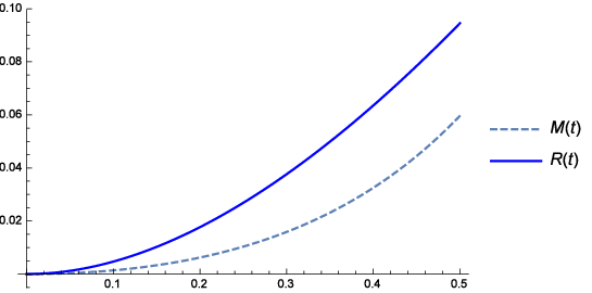
Let 0<t≤120<t\leq\frac{1}{2}, and define

(18) M⁡(t)\displaystyle M(t) =log⁡(t)−log⁡(|log⁡(1−t)|)−log⁡(1−t)+tt\displaystyle=\log(t)-\log(|\log(1-t)|)-\frac{\log(1-t)+t}{t}
(19) R⁡(t)\displaystyle R(t) =t−log⁡(1+t).\displaystyle=t-\log(1+t).

Then,

0<M⁡(t)<R⁡(t)<t2.0<M(t)<R(t)<t^{2}.

The proof of Lemma 4.3 is deferred until later in this section. We include the graph of M⁡(t)M(t) and R⁡(t)R(t) in Figure 4 for the reader’s convenience.
Refer to caption
Figure 4. The Functions M⁡(t)M(t) and R⁡(t)R(t)

Applying Lemma 4.3, we will show:

Lemma 4.4.

On ∂Vℓ\partial V_{\ell},

(20) N(y,k)|hℓ(z)|≫kℓexp(−k⋅M(1ℓ+1)).N(y,k)\left|h_{\ell}(z)\right|\gg\frac{\sqrt{k}}{\ell}\emph{exp}\left(-k\cdot M\left(\frac{1}{\ell+1}\right)\right).
Lemma 4.5.

For all z∈Vℓz\in V_{\ell},

(21) N(y,k)|β(z)|≪k2k​ℓ+kℓexp(−k⋅R(1ℓ+1)).N(y,k)\left|\beta(z)\right|\ll\frac{\sqrt{k}}{2^{k}\ell}+\frac{\sqrt{k}}{\ell}\emph{exp}\left(-k\cdot R\left(\frac{1}{\ell+1}\right)\right).

Theorem 4.2 will follow from Lemmas 4.1, 4.3, 4.4, and 4.5.

4.4. Proofs of Lemmas 4.4 and 4.5

Before beginning the proofs of Lemma 4.4 and 4.5, we must provide two facts that will aid us. If 0<u<10<u<1, then

(22) u−u22≤log⁡(1+u)≤u−u24.u-\frac{u^{2}}{2}\leq\log\left(1+u\right)\leq u-\frac{u^{2}}{4}.

Additionally, recall Stirling’s approximation: For n∈ℤ+n\in\mathbb{Z}^{+},

(23) Γ⁡(n)∼2​πn​(ne)n.\Gamma(n)\sim\sqrt{\frac{2\pi}{n}}\Bigg(\frac{n}{e}\Bigg)^{n}.
Proof of Lemma 4.4.

Consider two cases:

Top and Bottom Boundaries: Let y=yℓy=y_{\ell}. Note that, from the definition of hℓ​(z)h_{\ell}(z) and the triangle inequality,

N⁡(y,k)​|hℓ​(z)|≥(2​π​y​ℓ)kΓ⁡(k)​exp​(−2​π​ℓ​y)ℓ⋅|1−|fℓ+1​(z)fℓ​(z)||.N(y,k)\left|h_{\ell}(z)\right|\geq\frac{(2\pi y\ell)^{k}}{\Gamma(k)}\frac{\text{exp}(-2\pi\ell y)}{\ell}\cdot\Bigg|1-\bigg|\frac{f_{\ell+1}(z)}{f_{\ell}(z)}\bigg|\Bigg|.

In the next steps, we substitute k−1=2​π​y​ℓk-1=2\pi y\ell and apply (23), which implies

eℓ​(k−1e)k​1Γ⁡(k)≫kℓ.\frac{e}{\ell}\left(\frac{k-1}{e}\right)^{k}\frac{1}{\Gamma(k)}\gg\frac{\sqrt{k}}{\ell}.

Furthermore, we get an upper bound on |fℓ+1​(z)fℓ​(z)|\left|\frac{f_{\ell+1}(z)}{f_{\ell}(z)}\right| at y=yℓy=y_{\ell} using (22), namely

(24) |fℓ+1​(z)fℓ​(z)|=(1+1ℓ)k−1​exp​(−k−1ℓ)≪exp​(−k4​ℓ2).\left|\frac{f_{\ell+1}(z)}{f_{\ell}(z)}\right|=\left(1+\frac{1}{\ell}\right)^{k-1}\text{exp}\left(-\frac{k-1}{\ell}\right)\ll\text{exp}\left(-\frac{k}{4\ell^{2}}\right).

Recall that ℓ≤ϵ​k\ell\leq\epsilon\sqrt{k} for a sufficiently small ϵ>0\epsilon>0, so (24) is less than 12\frac{1}{2} (say). Then,

(25) N⁡(y,k)​|hℓ​(z)|≫kℓ,N(y,k)|h_{\ell}(z)|\gg\frac{\sqrt{k}}{\ell},

for y=yℓy=y_{\ell}. Letting y=yℓ+1y=y_{\ell+1}, by similar methods, we conclude that (25) holds.

Left and Right Boundaries: Let x=x0±12x=x_{0}\pm\frac{1}{2}. Then, let r1​(y)r_{1}(y) and r2​(y)r_{2}(y) be the magnitudes of the two terms in N⁡(y,k)​hℓ​(z)N(y,k)h_{\ell}(z):

r1​(y)\displaystyle r_{1}(y) =yk​ℓk−1​exp​(−2​π​ℓ​y)\displaystyle=y^{k}\ell^{k-1}\text{exp}(-2\pi\ell y)
r2​(y)\displaystyle r_{2}(y) =yk​(ℓ+1)k−1​exp​(−2​π​(ℓ+1)​y).\displaystyle=y^{k}(\ell+1)^{k-1}\text{exp}(-2\pi(\ell+1)y).

Note that, when x=x0±12x=x_{0}\pm\frac{1}{2}, we have that

N⁡(y,k)​|hℓ​(z)|=(2​π)kΓ⁡(k)​(r1​(y)+r2​(y)).\displaystyle N(y,k)\left|h_{\ell}(z)\right|=\frac{(2\pi)^{k}}{\Gamma(k)}\left(r_{1}(y)+r_{2}(y)\right).

We additionally see that r1​(y)+r2​(y)≥max​(r1​(y),r2​(y))r_{1}(y)+r_{2}(y)\geq\text{max}(r_{1}(y),r_{2}(y)). By elementary calculus, we note that r1r_{1} is strictly increasing on yℓ+1≤y≤yℓy_{\ell+1}\leq y\leq y_{\ell}. Furthermore, r2r_{2} is strictly decreasing for the same range of yy values. Thus, max​(r1​(y),r2​(y))\text{max}(r_{1}(y),r_{2}(y)) is minimized at y0y_{0}, and r1=r2r_{1}=r_{2} at y0y_{0}. Hence, if x=x0±12x=x_{0}\pm\frac{1}{2}, recall (15) and Lemma 4.3 to gain the following:

N⁡(y,k)​|hℓ​(z)|\displaystyle N(y,k)\left|h_{\ell}(z)\right| ≫(2​π​y0)kΓ⁡(k)​(ℓ+1)k−1​exp​(−2​π​(ℓ+1)​y0)\displaystyle\gg\frac{(2\pi y_{0})^{k}}{\Gamma(k)}(\ell+1)^{k-1}\text{exp}(-2\pi(\ell+1)y_{0})
=(k−1)k​(ℓ+1)kΓ​(k)​(ℓ+1)|log(1−1ℓ+1)|kexp(−(k−1))⋅\displaystyle=\frac{(k-1)^{k}(\ell+1)^{k}}{\Gamma(k)(\ell+1)}\left|\log\left(1-\frac{1}{\ell+1}\right)\right|^{k}\text{exp}(-(k-1))\;\cdot
exp​((k−1)​(ℓ+1)​(log⁡(1−1ℓ+1)+1ℓ+1))\displaystyle\qquad\qquad\qquad\text{exp}\left((k-1)(\ell+1)\left(\log\left(1-\frac{1}{\ell+1}\right)+\frac{1}{\ell+1}\right)\right)
=eℓ+1(k−1e)k1Γ⁡(k)exp(−k⋅M(1ℓ+1)−(ℓ+1)(log(1−1ℓ+1)+1ℓ+1))\displaystyle=\frac{e}{\ell+1}\left(\frac{k-1}{e}\right)^{k}\frac{1}{\Gamma(k)}\text{exp}\left(-k\cdot M\left(\frac{1}{\ell+1}\right)-(\ell+1)\left(\log\left(1-\frac{1}{\ell+1}\right)+\frac{1}{\ell+1}\right)\right)
≫(k−1e)k1Γ⁡(k)exp(−k⋅M(1ℓ+1)).\displaystyle\gg\left(\frac{k-1}{e}\right)^{k}\frac{1}{\Gamma(k)}\text{exp}\left(-k\cdot M\left(\frac{1}{\ell+1}\right)\right).

Using (23), we derive (20) in this case.∎

It will be helpful to note that a minor modification of the proof of Lemma 4.4 gives

(26) N⁡(y,k)​|hℓ​(z)|≪kℓ,N(y,k)\left|h_{\ell}(z)\right|\ll\frac{\sqrt{k}}{\ell},

in VℓV_{\ell} as well.

Proof of Lemma 4.5.

To begin, we note that |β⁡(z)|≤|fℓ+2​(z)|+|fℓ−1​(z)|+|ε1​(z)|+|ε2​(z)|+|δ⁡(z)|\left|\beta(z)\right|\leq\left|f_{\ell+2}(z)\right|+\left|f_{\ell-1}(z)\right|+\left|\varepsilon_{1}(z)\right|+\left|\varepsilon_{2}(z)\right|+\left|\delta(z)\right|. Now, we break the proof into three parts:

Part 1: Consider fℓ+2​(z)f_{\ell+2}(z) and fℓ−1​(z)f_{\ell-1}(z). In the region VℓV_{\ell}, N⁡(y,k)​|fℓ+2​(z)|N(y,k)\left|f_{\ell+2}(z)\right| has the greatest magnitude when y=yℓ+1y=y_{\ell+1}. Because of this, we use the substitution yℓ+1=k−12​π​(ℓ+1)y_{\ell+1}=\frac{k-1}{2\pi(\ell+1)} and Lemma 4.3 to obtain:

N⁡(y,k)​|fℓ+2​(z)|\displaystyle N(y,k)\lvert f_{\ell+2}(z)\rvert ≤(k−1)kΓ​(k)​(ℓ+2)​exp​(−(k−1))​(1+1ℓ+1)k​exp​(−k−1ℓ+1)\displaystyle\leq\frac{(k-1)^{k}}{\Gamma(k)(\ell+2)}\text{exp}(-(k-1))\left(1+\frac{1}{\ell+1}\right)^{k}\text{exp}\left(-\frac{k-1}{\ell+1}\right)
=eℓ+2(k−1e)k1Γ⁡(k)exp(−k⋅R(1ℓ+1))exp(1ℓ+1)\displaystyle=\frac{e}{\ell+2}\left(\frac{k-1}{e}\right)^{k}\frac{1}{\Gamma(k)}\text{exp}\left(-k\cdot R\left(\frac{1}{\ell+1}\right)\right)\text{exp}\left(\frac{1}{\ell+1}\right)
≪(k−1e)k1Γ⁡(k)exp(−k⋅R(1ℓ+1)).\displaystyle\ll\left(\frac{k-1}{e}\right)^{k}\frac{1}{\Gamma(k)}\text{exp}\left(-k\cdot R\left(\frac{1}{\ell+1}\right)\right).

Then, using (23), we find that

(27) N(y,k)|fℓ+2(z)|≪kℓexp(−k⋅R(1ℓ+1)).N(y,k)\lvert f_{\ell+2}(z)\rvert\ll\frac{\sqrt{k}}{\ell}\text{exp}\left(-k\cdot R\left(\frac{1}{\ell+1}\right)\right).

For N⁡(y,k)​|fℓ−1​(z)|N(y,k)\left|f_{\ell-1}(z)\right|, the function has the greatest magnitude when y=yℓy=y_{\ell} in the region VℓV_{\ell}. Then, we proceed in the same fashion as before to achieve the bound in (27) for N⁡(y,k)​|fℓ−1​(z)|N(y,k)\left|f_{\ell-1}(z)\right|. We find that the upper bound on N⁡(y,k)​|fℓ+3​(z)|N(y,k)|f_{\ell+3}(z)| is no larger than the upper bound on N⁡(y,k)​|fℓ+2​(z)|N(y,k)|f_{\ell+2}(z)| for yy in the region (12). This is similarly true for N⁡(y,k)​|fℓ−2​(z)|N(y,k)|f_{\ell-2}(z)| and N⁡(y,k)​|fℓ−1​(z)|N(y,k)|f_{\ell-1}(z)|, respectively.

Part 2: Let ε1​(z)\varepsilon_{1}(z) and ε2​(z)\varepsilon_{2}(z) be defined as in Section 4.2. By [RVY, p.18],

N⁡(y,k)​|ε2​(z)|≪Q⁡(k,2​π​(ℓ+3)​y),N(y,k)\left|\varepsilon_{2}(z)\right|\ll Q(k,2\pi(\ell+3)y),

and

N⁡(y,k)​|ε1​(z)|≪P⁡(k,2​π​(ℓ−2)​y),N(y,k)\left|\varepsilon_{1}(z)\right|\ll P(k,2\pi(\ell-2)y),

where Q⁡(s,x)Q(s,x) is the normalized incomplete gamma function and P⁡(s,x)P(s,x) is the complementary incomplete gamma function, defined by:

Q⁡(s,x)=1Γ⁡(s)​∫x∞ts​e−t​d​tt,P⁡(s,x)=1Γ⁡(s)​∫0xts​e−t​d​tt.Q(s,x)=\frac{1}{\Gamma(s)}\int_{x}^{\infty}t^{s}e^{-t}\frac{dt}{t},\qquad P(s,x)=\frac{1}{\Gamma(s)}\int_{0}^{x}t^{s}e^{-t}\frac{dt}{t}.

Using the results of [T], [RVY] derived

(28) Q⁡(s,x)≪exp​(−(x−s)24​s)+exp​(−|x−s|4).Q(s,x)\ll\text{exp}\left(-\frac{(x-s)^{2}}{4s}\right)+\text{exp}\left(-\frac{\left|x-s\right|}{4}\right).

Note that P⁡(s,x)P(s,x) is bounded above by (28) as well. Letting s=ks=k and x=2​π​(ℓ+3)​yx=2\pi(\ell+3)y, and using the inequality k−1ℓ+1≤2​π​y≤k−1ℓ\frac{k-1}{\ell+1}\leq 2\pi y\leq\frac{k-1}{\ell}, we have

x−s=2​π​(ℓ+3)​y−k≥2​kℓ+1+O⁡(1).x-s=2\pi(\ell+3)y-k\geq\frac{2k}{\ell+1}+O(1).

Thus, with (28), we derive

Q⁡(k,2​π​(ℓ+3)​y)≪exp​(−k(ℓ+1)2).Q(k,2\pi(\ell+3)y)\ll\text{exp}\left(-\frac{k}{(\ell+1)^{2}}\right).

The same bound holds for P⁡(k,2​π​(ℓ−2)​y)P(k,2\pi(\ell-2)y) as well. Since R⁡(t)<t2R(t)<t^{2}, the bounds on N⁡(y,k)​|ε1​(z)|N(y,k)|\varepsilon_{1}(z)| and N⁡(y,k)​|ε2​(z)|N(y,k)|\varepsilon_{2}(z)| are consistent with (21).

Part 3: Recall δ⁡(z)\delta(z) satisfies (11). Note that

(29) ∑b|nb<n(bn)k−1≤∑d>11dk−1=ζ⁡(k−1)−1≪12k.\sum_{\begin{subarray}{c}b\mid n\\ b<n\end{subarray}}\left(\frac{b}{n}\right)^{k-1}\leq\sum_{d>1}\frac{1}{d^{k-1}}=\zeta(k-1)-1\ll\frac{1}{2^{k}}.

The method of proof given in (26), Part 1, and Part 2, gives us the following bound in VℓV_{\ell}:

(30) N⁡(y,k)​∑n=1∞|fn​(z)|≪kℓ.N(y,k)\sum_{n=1}^{\infty}\left|f_{n}(z)\right|\ll\frac{\sqrt{k}}{\ell}.

(Note that [RVY] utilizes the triangle inequality.) Thus, from (30) and (29), we find that

N⁡(y,k)​|δ⁡(z)|≪k2k​ℓ.∎N(y,k)\left|\delta(z)\right|\ll\frac{\sqrt{k}}{2^{k}\ell}.\qed
Proof of Lemma 4.3.

Let 0<t≤120<t\leq\frac{1}{2}. By taking the derivative of R⁡(t)R(t), we find that R⁡(t)R(t) is strictly increasing on its domain. Using its power series expansion, we see that R⁡(t)≤12​t2<t2R(t)\leq\frac{1}{2}t^{2}<t^{2}. To show that M⁡(t)<R⁡(t)M(t)<R(t), we define w⁡(t)w(t) to be the infinite sum w⁡(t)=12​t+13​t2+14​t3+⋯w(t)=\frac{1}{2}t+\frac{1}{3}t^{2}+\frac{1}{4}t^{3}+\cdots. Then, M⁡(t)=R⁡(w⁡(t))=w⁡(t)−log⁡(1+w⁡(t))M(t)=R(w(t))=w(t)-\log(1+w(t)), and our proof will be finalized as long as w⁡(t)<tw(t)<t by the monotonicity of R⁡(t)R(t). Note that, for t<1t<1,

w⁡(t)≤12​t+13​(t21−t)<t.∎w(t)\leq\frac{1}{2}t+\frac{1}{3}\left(\frac{t^{2}}{1-t}\right)<t.\qed

5. Inequivalence of Zeros at Atkin-Lehner Cusps

In order to show inequivalence of zeros around certain cusps, we recall the theory of Atkin-Lehner involutions. We write N=q1​q2=Q​RN=q_{1}q_{2}=QR such that (Q,R)=1(Q,R)=1. An Atkin-Lehner involution WQNW_{Q}^{N} is given by

WQN=(Q​abN​cQ​d),\displaystyle W_{Q}^{N}=\begin{pmatrix}Qa&b\\ Nc&Qd\end{pmatrix},

where OPENa≡1​ (mod ​R)a\equiv 1\text{ (mod }R), OPENb≡1​ (mod ​Q)b\equiv 1\text{ (mod }Q) and detWQN=Q\det W_{Q}^{N}=Q.

Let χ1′\chi_{1}^{\prime} and χ2′\chi_{2}^{\prime} be primitive characters modulo q1′q_{1}^{\prime} and q2′q_{2}^{\prime}, respectively. We define q1=(q1′,R)⋅(q2′,Q)q_{1}=(q_{1}^{\prime},R)\cdot(q_{2}^{\prime},Q) and q2=(q1′,Q)⋅(q2′,R)q_{2}=(q_{1}^{\prime},Q)\cdot(q_{2}^{\prime},R). Factor each character uniquely as χ1′=χ1′(Q)​χ1′(R)\chi_{1}^{\prime}=\chi_{1}^{\prime(Q)}\chi_{1}^{\prime(R)} and χ2′=χ2′(Q)​χ2′(R)\chi_{2}^{\prime}=\chi_{2}^{\prime(Q)}\chi_{2}^{\prime(R)}, where χi′(Q)\chi_{i}^{\prime(Q)} has modulus (qi′,Q)(q_{i}^{\prime},Q), and similarly for RR. We define χ1=χ1′(R)​χ2′(Q)\chi_{1}=\chi_{1}^{\prime(R)}\chi_{2}^{\prime(Q)} and χ2=χ1′(Q)​χ2′(R)\chi_{2}=\chi_{1}^{\prime(Q)}\chi_{2}^{\prime(R)}, and note that χi\chi_{i} is a primitive character modulo qiq_{i}.

Weisinger showed in [W] that

Eχ1′,χ2′,k|WQN​(z)=cQ​Eχ1,χ2,k​(z),\displaystyle E_{\chi_{1}^{\prime},\chi_{2}^{\prime},k}\Big|_{W_{Q}^{N}}(z)=c_{Q}E_{\chi_{1},\chi_{2},k}(z),

for some constant cQc_{Q}. This allows one to study the behavior of Eχ1,χ2,k​(z)E_{\chi_{1},\chi_{2},k}(z) around the cusp at infinity in terms of the series Eχ1′,χ2′,k​(z)E_{\chi_{1}^{\prime},\chi_{2}^{\prime},k}(z) around the cusp at aR​c\frac{a}{Rc}. We will use this theory in the coming proposition.

Let 𝒦⁡(q2)\mathcal{K}(q_{2}) denote the region

𝒦(q2)={z=x+iy∈ℍ:y>1q2,−12<x≤12}.\displaystyle\mathcal{K}(q_{2})=\left\{z=x+iy\in\mathbb{H}:y>\frac{1}{q_{2}},\ -\frac{1}{2}<x\leq\frac{1}{2}\right\}.
Proposition 5.1.

For an Atkin-Lehner involution WQNW_{Q}^{N}, where Q≠1Q\neq 1, the image of 𝒦⁡(q2′)\mathcal{K}(q_{2}^{\prime}) under the involution WQNW_{Q}^{N} is disjoint with the region 𝒦⁡(q2)\mathcal{K}(q_{2}).

Proof.

We briefly state that we cannot have c=0c=0, since that would imply Q=1Q=1. Let z=x+i​y∈𝒦⁡(q2′)z=x+iy\in\mathcal{K}(q_{2}^{\prime}). Then

Im​(WQN​z)\displaystyle\text{Im}\left(W_{Q}^{N}z\right) =Q​y(N​c​x+Q​d)2+(N​c​y)2≤Q​yN2​c2​y2\displaystyle=\frac{Qy}{(Ncx+Qd)^{2}+(Ncy)^{2}}\leq\frac{Qy}{N^{2}c^{2}y^{2}}
=1R​c2​N​y<q2′R​c2​N≤q2′R​N.\displaystyle=\frac{1}{Rc^{2}Ny}<\frac{q_{2}^{\prime}}{Rc^{2}N}\leq\frac{q_{2}^{\prime}}{RN}.

Note that

q2′R​N≤1q2,\displaystyle\frac{q_{2}^{\prime}}{RN}\leq\frac{1}{q_{2}},

since

q2′​q2R​N=q2q1′​R=(q1′,Q)q1′⋅(q2′,R)R≤1.\displaystyle\frac{q_{2}^{\prime}q_{2}}{RN}=\frac{q_{2}}{q_{1}^{\prime}R}=\frac{(q_{1}^{\prime},Q)}{q_{1}^{\prime}}\cdot\frac{(q_{2}^{\prime},R)}{R}\leq 1.

Therefore Im​(WQN​z)∉𝒦⁡(q2)\text{Im}(W_{Q}^{N}z)\not\in\mathcal{K}(q_{2}). ∎

Corollary 5.2.

The zeros of Eχ1,χ2,k​(z)E_{\chi_{1},\chi_{2},k}(z) in 𝒦⁡(q2)\mathcal{K}(q_{2}) are Γ0​(q1​q2)\Gamma_{0}(q_{1}q_{2})-inequivalent to the image of the zeros of Eχ1′,χ2′,k​(z)E_{\chi_{1}^{\prime},\chi_{2}^{\prime},k}(z) under the Atkin-Lehner involution WQNW_{Q}^{N}.

Acknowledgements

The authors would like to thank Dr. Matthew Young for his immense support and guidance. Additionally, the authors are grateful to Nathan Green for his advice, Texas A&M University Department of Mathematics, and the National Science Foundation for funding the Texas A&M REU, grant DMS–1460766.

References

  • [DS] F. Diamond, and J. Shurman, A First Course in Modular Forms. Graduate Texts in Mathematics, 228. Springer–Verlag, New York, 2005.
  • [GS] A. Ghosh and P. Sarnak, Real zeros of holomorphic Hecke cusp forms. J. Eur. Math. Soc. 14 (2012), no. 2, 465–487.
  • [HS] R. Holowinsky and K. Soundararajan, Mass equidistribution for Hecke eigenforms. Ann. of Math. (2) 172 (2010), no. 2, 1517–1528.
  • [MV] P. Michel and A. Venkatesh, The subconvexity problem for G​L2GL_{2}. Publ. Math. Inst. Hautes Études Sci. No. 111 (2010), 171–271.
  • [N] P. Nelson, Equidistribution of cusp forms in the level aspect. Duke Math. J. 160 (2011), no. 3, 467–501.
  • [NPS] P. Nelson, A. Pitalé, and A. Saha, Bounds for Rankin-Selberg integrals and quantum unique ergodicity for powerful levels. J. Amer. Math. Soc. 27 (2014), no. 1, 147–191.
  • [RS-D] F. K. C. Rankin, and H. P. F Swinnerton-Dyer, On the zeros of Eisenstein series. Bull. London Math. Soc. 2 1970, 169–170.
  • [RVY] S. Reitzes, P. Vulakh, and M. P. Young, Zeros of certain combinations of Eisenstein series. To appear in Mathematika.
  • [R] Z. Rudnick, On the asymptotic distribution of zeros of modular forms. Int. Math. Res. Not. 2005, no. 34, 2059–2074.
  • [S] K. Soundararajan, Quantum unique ergodicity for SL2​(ℤ)\ℍ{\rm SL}_{2}(\mathbb{Z})\backslash\mathbb{H}. Ann. of Math. (2) 172 (2010), no. 2, 1529–1538.
  • [T] J. Temme, The asymptotic expansion of the incomplete gamma functions. SIAM J. Math. Anal. 10 (1979), no. 4, 757–766.
  • [W] J. Weisinger, Some results on classical Eisenstein series and modular forms over function fields. Thesis, Harvard University (1977).