Accurate correlation energies in one-dimensional systems
from small, system-adapted basis functions
Abstract
We propose a general method for constructing system-dependent basis functions for correlated quantum calculations. Our construction combines features from several traditional approaches: plane waves, localized basis functions, and wavelets. In a one-dimensional mimic of Coulomb systems, it requires only 2-3 basis functions per electron to achieve high accuracy, and reproduces the natural orbitals. We illustrate its effectiveness for molecular energy curves and chains of many one-dimensional atoms. We discuss the promise and challenges for realistic quantum chemical calculations.
I Introduction
Many tens of thousands of electronic structure calculations are performed each year, the vast majority in a single-particle basis set of some sort. These calculations can be divided into two types: those that extract the energy from a set of single-particle occupied orbitals (denoted single-determinant) such as density functional theory (DFT) [1, 2, 3, 4, 5] or Hartree Fock (HF), and those that go beyond a single determinant, such as configuration interaction, [6, 7] coupled cluster methods, [8, 9, 10] density matrix renormalization group (DMRG), [11, 12, 13, 14, 15, 16] and some types of quantum Monte Carlo. Going beyond a single determinant is necessary for many systems, but is typically much more demanding computationally. Such calculations are more difficult because larger basis sets are needed to achieve chemical accuracy (1 kcal/mol), and computation times usually scale as a high power of the number of basis functions. These larger basis sets are needed to represent the electron-electron cusp in the wavefunction which exists at every point in space.
A natural question arises: what would be the optimal basis set for an electronic structure calculation, assuming the basis is specifically adapted to that system? For a single-determinant method, the answer is clear: the self-consistent occupied orbitals are the optimal basis for that calculation: used as a basis, they reproduce the exact energy and properties. The number of these basis functions (for a spin-restricted calculation) is thus , where is the number of electrons. Of course, this minimal basis does not offer a computational shortcut: the occupied orbitals must be determined in a separate, non-adapted basis calculation. Here, we are concerned with multi-determinant methods, and we will assume that the computation time for a traditional single-determinant calculation is small in comparison to the multi-determinant method.
For post-HF methods, there is no exact finite system-adapted basis: any finite basis introduces errors. However, the natural orbitals are close to the most rapidly converging single-particle basis, at least in terms of allowing the greatest possible overlap with the exact ground state.[17, 18] The natural orbitals are the eigenstates of the single-particle density matrix (also known as the equal-time one-particle Green’s function). The number of nonzero eigenvalues (occupancies) is infinite. A (near) optimal basis of orbitals consists of the natural orbitals with the greatest occupancy.
One obvious weakness in using natural orbitals is that one does not know them until after one has solved the interacting system, using a post-HF method, with another larger basis. Iterative natural orbital methods are a way to reduce the computational expense, but approximate natural orbitals that did not need a post-HF method to determine them could be very useful.[19] But natural orbitals have another key weakness: they are (normally) completely delocalized across the system. This delocalization prevents a number of shortcuts that can greatly decrease computation times for large systems. Delocalization is especially harmful for low-entanglement methods such as DMRG, since there is no area law for the entanglement entropy in a delocalized basis.[20]
Here we describe an approach that starts with the occupied orbitals of a DFT (or HF) calculation, and yields basis sets which produce high accuracy in correlated calculations. We test this approach in 1D, using potentials that make 1D mimic 3D in many respects, and using DMRG.[21] The computational effort for the basis construction is minimal. The number of basis functions needed is typically about , where is the minimal number of natural orbitals needed to reach high accuracy, or about two or three times the number of electrons. We expect this method can be easily extended to quasi-1D systems (such as large- atoms or chains of real H atoms) and hope it can be applied more generally in 3D.
The first step produces what we call “product plane waves” (PPWs) by multiplying the occupied orbitals by a set of low momentum cutoff plane waves. The lowest momentum is determined by the spatial extent of the entire system. This simple ansatz converges well in our tests in 1D, and we show how its convergence is within about a factor of 2 compared to natural orbitals. But a weakness of PPWs, shared with natural orbitals, is that the basis is not local. As the second major part of this work, we describe fragmentations of the PPWs that utilize wavelets[22, 23, 24, 25, 26, 27, 28, 29, 30, 31, 32, 33, 34, 35, 36, 37, 38, 39, 40, 41, 42, 43, 44, 45, 46, 39, 47, 34, 48, 49, 50, 51, 52, 53, 54, 55, 54, 56, 57, 58, 59, 60, 61, 62, 63, 64, 65, 66] to produce atom-centered adapted orthogonal bases with good completeness and locality. This approach requires only a modest additional number of basis functions to yield the same accuracy as PPWs, but with a smooth, local, and orthogonal basis.
II Background
II.1 The one dimensional Hamiltonian
Our non-relativistic many-electron Hamiltonian, expressed in second quantized form, either in a basis set or on a grid, is[67, 68]
| (1) |
with fermionic operators labeled either by site or basis-function and with spin (or ). We define the ‘exact’ solution as solving this Hamiltonian on a very fine grid, which is close to the continuum limit.[69, 21] For both the grid and for basis functions, we find the exact many-particle ground state of these 1D reference systems using DMRG. The one-electron integrals are
| (2) |
where for the 1D calculations, is the external potential, discussed below. In a basis, with functions , the two-electron integrals are
| (3) |
On a grid, the interaction takes a much simpler diagonal form with and , with the integral taking the value . For grid calculations, we use the ITensor library, along with matrix product operator technology.[70] In the basis, we use the Block DMRG code since it is specifically tailored to avoid stationary states that are not the ground state in a basis set and has implemented the form of the Hamiltonian efficiently. [14, 71, 72, 73, 74]
Previously, we have explored 1D potentials which mimic as closely as possible the behavior of real 3D systems. A particularly convenient choice matching a number of 3D features is a single exponential function, with and , and , where is the atomic number, just as in 3D. This particular function closely mimics the results from a soft-Coulomb interaction, but at a reduced cost for grid DMRG calculations.[21, 70] This potential also more closely mimics 3D since it has a mild singularity at zero distance. In 3D, the Coulomb interaction is divergent, but its effect is moderated, and integrals over it are finite, because of the very small volume associated with the region, and the associated integration factor . In 1D, we get qualitatively similar behavior from the slope discontinuity in the potential at . A local density approximation (LDA) was also derived for this interaction. Our finite difference grid Hamiltonian looks like an extended Hubbard model,[69]
| (4) | |||||
where the superscript “fine” indicates we will use this lattice on the finest (original) grid of spacing , , external potential , and long-ranged electron-electron interaction on sites and . A distance of 60 from the outermost grid points to the first or last atom is used for all systems that follow, allowing wavefunctions to have extended tails.

The natural orbitals are the eigenvectors of the one-particle reduced density matrix (RDM), which is the equal-time one-particle Green’s function, with matrix elements:
| (5) |
The eigenvalues of are the occupation numbers and the eigenvectors are the natural orbitals, which we order in decreasing occupation. Fig. 1 shows the first two for 1D He, and we later show (Fig. 3) that, in a basis set of these 2 orbitals alone, the expectation value of the Hamiltonian is only 1 kcal/mol above the exact ground-state energy. We use the term high accuracy to indicate errors of less than 1.6 mHa, which corresponds to the 1 kcal/mol criterion commonly called “chemical accuracy” in quantum chemistry.
II.2 Wavelets
Wavelets were originally introduced by Haar in 1910[22] but they have since been modernized and expanded by several works by Gabor, [23] Grossman and Morlet,[24] Meyer,[25] Mallat,[26] and Daubechies[27, 28, 29] and many others. These functions have become widely used in audio and image compression (such as jpeg and mp3 file formats). These were also connected to a quantum gate structure, tensor network algorithms, and compression of matrix product states.[58, 59, 60]
Consider a localized function located near the origin. We can form a basis from this function by translating it by all integer translations, i.e., for integer . A wavelet transformation (WT) is a mapping of to an new function defined by
| (6) |
where is the dilation factor, which is normally taken to be 2. The WT is defined by the coefficients . We will only consider compact wavelets, for which the number of nonzero ’s is finite. The scaling function of the WT, , is the fixed point of this mapping. The are chosen cleverly to make the to be orthogonal for different , and to have a number of other desireable properties, such as polynomial completeness up to a certain order.[27] The scaling function is designed to represent smooth, low momentum parts of functions. The scaling function is not a wavelet, although it does form the top layer of a wavelet basis. A wavelet is formed from using another set of coefficients (which are defined in terms of the ):
| (7) |
The wavelets capture higher momentum features.
A wavelet basis consists of scalings and translations of and , and it is complete and orthonormal. It is characterized by a coarse grid with spacing . At all integer multiples of , one puts a scaling function, of size , namely . Then, at scales , , , etc., one puts down a grid of scaled wavelets, with the spacing and the size of the functions always equal. All these functions together are complete, and they are all orthogonal to each other. Some of the functions of a wavelet basis are shown in Fig. 2.

Wavelet bases are an attempt to have locality in both space and momentum simultaneously, as much as possible, subject to the constraint of orthgonality. The layer of scaling functions represent all momenta from 0 to roughly ; the coarsest layer of wavelets represents momenta from roughly to , etc., but with significant overlap in the momentum coverage between different layers.
We have briefly described wavelet bases in terms of continuous functions, but they can equally be described in terms of WTs acting on an initial fine grid. The WTs we use are based on the fine grid used by the grid DMRG calculations, and these are what is shown in Fig. 2.
Many different types of wavelet transforms have been constructed. Here we choose Coiflets, derived by Daubechies,[27] which are characterized by the number of nonzero . We choose relatively high to get good completeness and smoothness. Wavelets can be easily extended to higher dimensions by taking products such as ,[61] so the principal features of 1D carry over to 3D.[75, 76, 77, 78, 76, 79, 80, 81, 56]
III Product Plane Waves
In this section, we describe our new approach to design a specific system-dependent basis with as few functions as is practical. We first argue that the exact natural orbitals provide a natural least possible number, but rely on knowing the exact solution.[17, 18] We then show how to combine planewave-type basis functions (PPWs), wavelet technology, and adaptation via approximate DFT (or other) single-particle orbitals, to create a basis with no more than about twice this number, but still yielding high accuracy. A crucial feature is that we never use more than a few of each kind of function, so that we never come close to being limited by the asymptotic convergence properties of any one set of basis functions. Further, the initial orbitals do not need to be obtained to high accuracy. The purpose of these orbitals is to find the important features (where the density is large) features of the system to act as a scaffold for the following calculations. These orbitals can be obtained quickly at a low accuracy.
III.1 Natural orbitals as a basis
We wish to find basis sets that, when solved exactly, give ground-state energies of high accuracy, i.e., no more than 1 kcal/mol above the exact, complete basis limit. We wish to find basis sets that converge to this accuracy with as few functions as possible, but also without needing to know the exact solution to determine them. With the fine grid DMRG wavefunction, we can calculate exactly and find the exact natural orbitals. Since our DMRG solutions do not break spin symmetry if the number of electrons is even, the up and down RDMs are identical. (For odd electron numbers, we average the up- and down-RDMS and use that to define our natural orbitals.)

The first two natural orbitals for a 1D helium atom were shown in Fig. 1. The natural orbitals yield the smallest number of basis functions that can be expected to yield high accuracy, i.e., when ordered by occupancy, the least number which, when used as a basis, yields an error below high accuracy. Fig. 3 shows the energy error for a variety of systems, when the basis is chosen as a finite number of the most occupied exact natural orbitals. We see that for 1D He, but is 3 for 1D H2 either close to equilibrium () or stretched (). For 1D Li, , while 1D Be has . Unstretched 1D H4 also has , but stretched 1D H4 requires . Thus increases with the number of electrons, and also (slightly) with the number of centers.

III.2 Constructing the basis
Given the orbitals from a HF or DFT calculation, perhaps the simplest conceivable basis would be the occupied HF or DFT orbitals, since this allows the reproduction of the single determinant. One well-known approach for enlarging this basis to allow for correlation is to use additional eigenstates of the Fock matrix, selected by an energy cutoff.[82, 81, 42, 81] It is clear, however, that this eventually becomes inappropriate. For a more complete basis, one needs functions with positive energy, but there are an infinite number of functions at zero energy far from the molecule. To remedy this, we could put a box around the molecule and include only functions within that box. However, this can be very wasteful, since the box needs to include extended tail regions, where additional basis functions are not very useful. Instead of using energies, we adopt a quite different approach, motivated by the construction of variational wavefunctions—in particular, Jastrow functions.
Single-particle determinantal states from DFT or HF are rough approximations to the many-particle wavefunction, but can be improved substantially by multiplication by a Jastrow factor, , which provides explicit correlation. Modifying a determinantal wavefunction with a Jastrow factor is often the first step in designing a variational wavefunction for quantum Monte Carlo calculations[83] The Jastrow factor acts as a multiplicative factor for the wavefunction and simple form for is[84]
| (8) |
The term is near 1 if and are far away, and becomes less than one as and come together, building in the electron-electron cusp. We now ask the question: what would be a good single-particle basis to represent or ?
The fact that is a function of the difference of two position vectors means that there is no benefit to increasing resolution in one region relative to another, at least for fitting . One does expect, however, that longer wavelength functions are more important than short wavelength functions. This suggests that a plane wave basis, restricted to the general vicinity of the molecule, with a momentum cutoff which is not too high, is a reasonable approximate basis for a Jastrow function.
Since the Jastrow function in a variational wavefunction multiples the determinant of occupied DFT orbitals, this suggests a very simple ansatz for a basis for correlated calculations: the product of occupied orbitals and low momentum cutoff plane waves, which we call a product plane wave (PPW). To be more specific: let be a set of plane waves with a low momentum cutoff, and let be the occupied orbitals from a DFT/HF calculation. Then our product plane-wave (PPW) basis is . The momentum cutoff in corresponds to some minimal resolution. Linear combinations of the can represent a correlation hole at any position within the system, while high momentum behavior near the nuclei is captured by the . , so that the themselves are part of the basis.
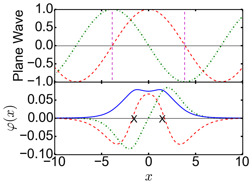
In generating a PPW basis, several choices must be made. First, we want to put the molecule in a “box” that defines the sequence of momenta in the plane waves. Since the detailed correlations we want from the plane waves are weak in the tails, and since the box size is only used to define momenta, we do not include long density tails. We simply choose a small density cutoff, , to define the edge of our box, from our DFT (or HF) calculation. Here throughout, but we expect our qualitative results to be very insensitive to this choice. For neutral atoms, the corresponding box sizes are and for to . A simple example of a product plane wave basis is illustrated in Fig. 5. The first two functions resemble the natural orbitals of 1D He in Fig. 1 and the natural orbitals here. This resemblence between PPWs and NOs tends to continue for higher functions, although the precise order of the functions can vary.

Let be the number of occupied orbitals in a DFT or other approximate calculation. Let be the width of the box defined by the cutoff . Then choose an integer to create functions, the identity and and , where , , and multiply each by the occupied DFT orbitals, creating primitive PPWs. Next, we exactly orthogonalize these orbitals via the Gram-Schmidt process, in the order of -values, starting with the identity. The results for 1D H4 are shown in Fig. 6 and compared to the exact natural orbitals. These orthogonalized PPWs are remarkably close to the exact natural orbitals, especially for those orbitals that are occupied in the DFT calculation, but also even for those that are not. (The additional wiggle in the 4th PPW is due to the orthogonalization procedure).

Finally, in Fig. 7, we show the energies for our systems as a function of the number of (orthogonalized) PPWs. For 1D He and 1D H2, , so increasing by 1 yields two more PPWs (the sine and the cosine); for the rest, , and 4 PPWs are added each time. A quick glance shows a remarkable similarity to the ordered natural-orbital energy errors of Fig. 3. The PPW functions yield high accuracy with a few more functions than , showing that they do not just look similar to the NO’s, they are similar in an energetically meaningful sense. We denote as the least number needed to reach high accuracy. A more careful inspection shows that they are not quite as accurate, even for 1D He, and that the difference grows with the number of electrons and the number of atoms. It is most noticeable for stretched 1D H4, where , whereas . But this is still a remarkably small number for a strongly correlated system.
IV Wavelet localization
So far, we have accomplished our goals of a basis function set with a low number of orbitals. Our PPWs yield high accuracy with about basis functions. But, to be efficient, tensor network methods such as DMRG require the low entanglement that comes from localized basis sets. Other methods may also benefit from localized basis functions, which make Hamiltonians sparse. Now we study cases with more than one atom, showing how we can use wavelet technology to break down a PPW into localized, smooth orthogonalized basis functions, centered around each atom, without too large an increase in the number of functions.
Traditional methods for localization rely on orthogonal transformations within the set of basis functions one already has. Not enlarging the set of functions puts a strong limit on how localized the functions can be made. However, if one enlarges the space without limit, one can make the basis as local as one wishes. One can think of “chopping up” each delocalized basis function (which we can picture as a molecular orbital): partition all of space into a chosen number of disjoint regions, or cells.[86, 87, 88, 89, 88, 90, 91] For example, one can make the number of cells the same as the number of atoms, and define each cell by associating each point in space with the closest nucleus. Form a basis by projecting each delocalized basis function into each cell, i.e. multiplying it by a function which is unity for points in the cell and zero outside, and repeating for all delocalized functions. Linear combinations of chopped up functions would allow one to reproduce any of the original delocalized functions, but this would make a terrible basis, for two reasons: 1) discontinuous basis functions have infinite kinetic energy, and 2) the number of localized functions scales as the square of the number of atoms.
Using wavelets, we can retain this idea of “chopping up” basis functions into different regions, but fix these two problems. As discussed in II.2, we define a complete wavelet basis consisting of a grid of scaling functions with lattice spacing (say with Bohr), and an infinite sequence of wavelets at scales , , , etc, as shown in Fig. 2. We will refer to any of these functions, either a scaling function or a wavelet of any scale, as a WF (wavelet-function).
Now to chop up a delocalized basis: expand all delocalized functions in terms of the WFs. Many WFs will not have significant overlap with any functions, and can be dropped. This procedure thus produces a localized but smooth basis encompassing the original functions, assuming one has chosen smooth wavelets. However, the number of functions tends to be rather high, so we use this only as a starting point.
Again we partition all of space into cells, associated with atoms. Associate each WF to a cell. A natural way to do this is to define a center of mass for each function, and then the WF goes in the cell that contains its center of mass. Now we can project each delocalized function into each cell, simply by expanding the function in terms of the WFs belonging to the cell. This cuts the delocalized function into pieces which are all orthogonal. An example of this procedure is shown in Fig. 8.
If we repeat this with additional delocalized functions, the pieces in different cells will be orthogonal, even if they came from different delocalized functions, since the WFs of different cells are orthogonal. Within a single cell, the pieces will not be orthogonal, and may have substantial overlap. The final step is to recombine all the pieces in a particular cell into a reduced set of orthogonal functions for that cell, and repeat for all cells. Note that while the original delocalized functions may be normalized, the pieces come from a projection and will not be, and some pieces may have very small normalization. It is important to leave the pieces unnormalized. For each cell, we wish to find the minimal set of basis functions that can represent all the pieces to within a specified accuracy. This is a well known linear algebra problem with a simple solution. Let be the piece of delocalized function , expanded in terms of the WFs belonging to a cell . Form a cell covariance matrix as
| (9) |
Then the reduced basis we seek is the set of eigenvectors of (which is positive semi-definite) with eigenvalues above a specified cutoff, . This cutoff is roughly the mean-square error in representing all the different pieces. This is often called a principal component analysis. [92, 93, 94, 95, 85] Here we call the entire process wavelet localization (WL) and the resulting basis functions wavelet-localized orbitals (WLOs). Although the WLO procedure could be applied to other delocalized bases, here we will only consider its application to PPWs.

Fig. 9 shows the results of wavelet localization for 1D H4, with a spacing , discussed more in Sec. IV.1. For simplicity, the figure shows only the two leading eigenfunctions and their eigenvalues for only cells 1 and 3. The dashed lines show the dividing lines between the different boxes; the nuclei are at , , , and . The functions are all orthogonal, with oscillations in the tails of each function to ensure orthogonality between boxes.
The parameter , the spacing of the scaling functions, is crucial, as it sets the size of the region in which functions on adjacent boxes overlap. In the limit , this chopping up procedure reduces to the naive discontinuous procedure mentioned at the beginning of this section. The procedure also becomes poorly behaved if is larger than the interatomic spacing. Roughly, one should set to a modest fraction of the interatomic spacing, but later on we show results as a function of to determine optimal values.
Lastly, we note that, for multi-center stretched systems, if , the box for an atom, then we use instead of for that cell. This can greatly increase the number of functions to , where is the number needed to reach high accuracy for the isolated atom, but unneeded functions will be discarded by our wavelet localization.
IV.1 Performance of WLO bases
In this section, we wish to check that our WLOs work well for some correlated quantum calculations, and find out how many WLOs are needed for a given task. Our procedure requires, at most, functions. Thus, for a H4 chain that is unstretched (no spin-symmetry breaking), , we will usually choose , and have 4 cells. A PPW calculation has 6 functions, and up to 24 (6 per cell) when fragmented. However, in practice, up to half those functions can be eliminated by the cutoff of our covariance matrix. This removal of irrelevant functions becomes increasingly important as the number of atoms grows.

The prototype calculation is the dissociation of molecular hydrogen. All single-determinant methods fail as bonds are stretched and electrons localize on distinct sites. Molecular hydrogen dissociates into an open-shell biradical (two 1D H atoms). The molecular energy as a function of separation is given in Fig 6 of Ref. 21. That figure also shows the failure of LDA, with a Coulson-Fischer point[96] , where the unrestricted broken symmetry solution becomes lower in energy than the spin-singlet within LDA. In Fig 10, we show the error in the energy curve, using pure PPWs, and also separating into separate cells, using and .
Beginning with the PPWs (dashed lines), we see that increasing improves accuracy systematically, as expected. Moreover, for a given or higher, we see that the error increases systematically as the bond is stretched until is reached. This is because the LDA orbital is becoming less and less close to the exact natural orbital as the bond is stretched. Beyond this point, there is a great decrease in error, as the the number of LDA orbitals doubles (due to spin-symmetry breaking). Even the largest PPW basis shown here () does not achieve high accuracy close to the CF point. But our WLOs do reach high accuracy everywhere for , and almost everywhere with , using functions for , and double that beyond. (The wavelet localization does not throw out any WLOs here.) Thus our basis set works, even through the CF point. Of course, in practice, quantum chemists want forces, and some smoothing procedure would be adopted to avoid the kink at the CF point.
The strong changes with in the error in the red curve past the CF point can be attributed to the grouping of the scaling and wavelet functions. As the bond is stretched, because the functions are fixed in real space, some of the functions are assigned to the left cell, and others to the right. This assignment can change suddenly, causing a drop in the eigenvalue weights in the covariance matrix of one of the cells and decreasing the number of functions. Note that this effect occurs only for errors far below the high accuracy threshold.

Next we consider performance for longer chains of 1D H atoms. Now the covariance cutoff becomes important for curtailing the total number of functions. Figure 11 illustrates the effect of the covariance cutoff for H4 near equilibrium. The higher the value of , the more functions are thrown away, but the greater the error is. If is set too small, then no functions are removed, not even those that have essentially no effect on the energy. The figure shows that the full basis has an error of about 0.1 kcal/mol. But high accuracy is achieved with and only 14 functions. This is to be contrasted with from Fig 3 and from Fig. 7. In this case (near equilibrium), the WLOs form a near-complete localized orthogonal basis with no more functions than PPW, and with lower error. Note that setting does not add in any more functions.
| 0.5 | 16 | 0.24 | 16 | 0.33 | 26 | 0.11 | 24 | 0.09 | 23 | 0.21 |
|---|---|---|---|---|---|---|---|---|---|---|
| 1.0 | 14 | 0.43 | 16 | 0.26 | 24 | 0.15 | 22 | 0.11 | 22 | 0.16 |
| 2.0 | 16 | 0.37 | 15 | 1.50 | 28 | 0.04 | 25 | 0.08 | 24 | 0.15 |
| 4.0 | 18 | 0.34 | 18 | 0.52 | 29 | 0.04 | 25 | 0.10 | 25 | 0.17 |
To see the effect as a function of bond length, in Table 1, we give energy errors and numbers of basis functions for various values of and several values of , for a calculation with . (In all cases, was found to yield errors higher than 1 kcal/mol.) We see that the least number of functions needed occurs for , especially as the chain is stretched.
| 42 | 0.47 | 51 | 0.10 | 50 | 0.63 | 49 | 0.25 | |
| 42 | 0.47 | 43 | 1.29 | 49 | 1.08 | 40 | 0.83 | |
Finally, we have run examples of 10-atom chains. We achieve high accuracy for , throughout the range of shown in the table, with about 5 functions per site when . This may seem like a large number of functions, but keep in mind that, as increases, this is a strongly correlated system tending toward its thermodynamic limit. Moreover, we have required our total energy to be accurate to 1 kcal/mol all along the curve, not just the energy per atom. One would also expect most energy differences to converge more rapidly than the total energy. Table 2 also illustrates the benefits of the covariance cutoff. By setting its value to , we significantly reduce the number of functions as increases, but in the middle, our error is slightly greater than 1 kcal/mol. For many practical purposes, this should be sufficient, but the larger lesson is that, for any desired application, there is a controllable trade-off between accuracy and number of functions.

We end with a heteronuclear diatomic, 1D LiH, to show that our method still works in the absence of left-right symmetry. Fig. 12 was calculated with and . The LDA orbitals remain an excellent starting point for approximating the NO’s, and the NO’s in the WLO basis are identical (on this scale) to the exact NO’s. The energy error is only 1.04, using 11 basis functions.
V Discussion and conclusions
We have presented algorithms to generate a basis set that is adapted to a specific molecular system and designed to be used in correlated calculations. The basis begins with an inexpensive DFT or HF calculations, and the generation of additional functions from the occupied orbitals to allow correlation is even less expensive. A product plane wave (PPW) ansatz adds additional functions using a product of low momentum plane waves times each occupied orbital. In our 1D test systems, this ansatz produces results within high accuracy using about twice as many functions as in an ideal natural orbital basis. Then, to generate basis functions localized near each atom, we introduced a wavelet localization procedure. Compared to standard localization methods, which involve an orthogonal transformation of the existing functions without expanding the basis, wavelet localization produces stronger localization with much smaller orthogonalizing tails, at the expense of adding basis functions. This procedure is particularly useful for DMRG calculations, where locality in the basis is an important criteria. It may also improve scaling on large systems in other correlation approaches. Our method, as presented here, should allow much larger systems to be treated than previously possible in our 1D mimic of realistic electronic structure (such as the 100-atom chains of Ref. 97).
Our procedure has only been given and tested upon a 1D mimic of the 3D world. A naive generalization of PPW to arbitrary 3D problems would involve many more plane waves, roughly the cube of the number in 1D. For a fixed momentum cutoff the number of plane waves also grows with the length of the system, even in 1D. This would appear to generate far too many functions to be practical, but the wavelet localization would counteract this effect. We can think about how this works by considering one particular cell, centered on an atom. The PPW basis generates occupied orbitals times plane waves with a low momentum cutoff. The number of functions needed to span this set in one cell should not be too large, since the only high frequencies present are from the cusps of the occupied orbitals at the nuclei, which in a Gaussian basis can be represented by a small number of basis functions. Otherwise, there are only a limited number of low frequency modes in a single atom cell. This means that there must be significant redundancy in the PPW functions, particularly for many electrons. The principle component analysis of the wavelet localization would remove this redundancy. This makes it clear that except for very small molecules, one should not apply PPW on its own, but in conjunction with wavelet localization. Nevertheless, there are likely significant challenges in going to 3D which we must leave for future work. In 1D, our bases give high accuracy with only about twice as many functions as in an equivalent natural orbital basis. It seems reasonable that a variation of our 1D approach can be found for 3D which is similarly less efficient than a natural orbital basis by only a modest factor.
In the case of a He atom, this means roughly that 3D He would need about the cube of the number of functions as 1D He. This argument would apply to any basis, including natural orbitals. Indeed, one finds one needs about 15 NOs for chemical accuracy in 3D He,[98] versus 2 or 3 for 1D He. Our PPW basis does not try to beat the NOs, which is not possible; rather, it tries to duplicate their completeness but based on a cheap calculation. In 1D, we obtain the same accuracy as with an NO basis if we use about twice as many functions. In 3D, we hope to do similarly–but this has not been tested.
One improvement to our PPW approach which we have not explored here is to give more weight to the occupied orbitals than to the additional functions coming from the plane waves with nonzero momentum. This would be fairly simple to implement in our wavelet localization, by multiplying the functions by a weighting factor less than 1. One would expect this natural modification to further reduce the number of functions needed for high accuracy. We also note that our procedure could also be applied without chopping, but still removing irrelevant basis functions, by constructing the orthonormal basis from the PPWs
| (10) |
where is the overlap matrix of the . Now , so the principle component analysis consists of forming a basis of the eigenvectors of the overlap matrix with the largest eigenvectors, up to cutoff . This procedure reduces basis-set linear dependence; here it might reduce the PPW basis size significantly without much loss of accuracy.
A number of existing approaches also utilize or are based on approximate natural orbitals. For example, some Gaussian basis sets attempt to reproduce properties of atomic natural orbitals.[99] A key difference with our approach is that we start from the beginning with orbitals adapted to the specific molecule under consideration, based on a DFT or HF calculation. It would be interesting to compare the number of functions needed to reach chemical accuracy in 3D between our PPW approach and standard Gaussian basis sets. (We do not have these Gaussian basis sets for our 1D test systems.)
Another common approach is to find approximate natural orbitals from a low-order correlation calculation, such as second order perturbation theory, e.g. MP2.[100] Our PPW method is simpler and faster, and it would be interesting to compare the accuracy of these two approaches. One might also combine them: in cases where the perturbation calculation was expensive to do in a large basis, one might first get a PPW basis, which would be much smaller than an unadapted basis, and then refine it further by getting approximate natural orbitals with a perturbation theory approach.
The localization using wavelets could be applied in a broader context than we have used here, such as to standard Gaussian bases or to approximate natural orbitals coming from a low order correlation method. This could potentially improve the performance of DMRG or other tensor network methods. By improving the sparsity of the Hamiltonian, it may also improve the computational scaling for DFT on large systems. In particular, using wavelet localization to impose locality only at the atomic level may be more efficient than existing wavelet approaches which do not recombine the wavelets into a smaller number of functions. Specifically, one could wavelet filter a standard Gaussian basis to produce an orthogonal basis with more locality and sparsity than traditionally localized Gaussian bases.
Since we are trying to produce basis sets for correlated calculations, where basis set convergence is slower than for DFT or HF calculations, we must think about the effect of the basis on the electron-electron cusp. Our choice of 1D potential interaction, which has a slope discontinuity at the origin, is designed to partially mimic the electron-electron cusp behavior in 3D. In 3D, the potential diverges as , but the effect is substantially reduced by the 3D volume element. The moderate singularity we have in 1D is similar, but we cannot expect our results to match 3D precisely. Also, when trying to achieve chemical accuracy, the short range cusp behavior is thought to be less relevant than intermediate distance electron-electron correlation. This further complicates the comparisons between 1D and 3D, and a 3D procedure and benchmark calculations are clearly needed.
Another difficulty in implementing our approach in 3D is the computation of the integrals defining the Hamiltonian, once the basis is defined. In our 1D implementation, all integrals are written in terms of sums over the fine grid; this would not be practical in 3D. Wavelet bases, which are a crucial part of our wavelet localization, are able to represent nuclear cusps more efficiently than grids, so one might try to work directly in the wavelet basis, expressing all the final basis functions as linear combinations of wavelet functions.[32, 57, 37] However, wavelets are much less efficient than atom-centered Gaussians for representing nuclear cusps, and so a much more efficient approach might be to try to combine wavelets with a few Gaussians per nucleus. Another approach to dealing with nuclear cusps would be to use pseudopotentials, so there are no cusps. Yet another is to employ a basis set that inherently has a one dimensional structure.[86, 87, 101, 102] We leave this set of 3D implementation problems for future work.
VI Acknowledgements
This work was supported by the U.S. Department of Energy, Office of Science, Basic Energy Sciences under award #DE-SC008696. T.E.B. also thanks the gracious support of the Pat Beckman Memorial Scholarship from the Orange County Chapter of the Achievement Rewards for College Scientists Foundation. T.E.B. graciously thanks Professor Filip Furche, Dr. Shane Parker, Dr. Vamsee K. Voora, and Sree Balasubramani for their patience in explaining and introducing methods from quantum chemistry. Access to and discussion about the Block code was provided to T.E.B. by Professor Garnet K. Chan and Professor Sandeep Sharma, both of whom we thank.
References
- [1] P. Hohenberg and W. Kohn, “Inhomogeneous electron gas,” Phys. Rev. 136, B864–B871 (1964).
- [2] W. Kohn and L. J. Sham, “Self-consistent equations including exchange and correlation effects,” Phys. Rev. 140, A1133–A1138 (1965).
- [3] Kieron Burke and Lucas O. Wagner, “Dft in a nutshell,” Int. J. Quant. Chem. 113, 96–101 (2013).
- [4] K. Burke, “Perspective on density functional theory,” J. Chem. Phys. 136, 150901 (2012).
- [5] Aurora Pribram-Jones, David A. Gross, and Kieron Burke, “Dft: A theory full of holes?” Annual Review of Physical Chemistry 66, 283–304 (2015).
- [6] C David Sherrill and Henry F Schaefer, “The configuration interaction method: Advances in highly correlated approaches,” Advances in quantum chemistry 34, 143–269 (1999).
- [7] Christopher J Cramer, Essentials of computational chemistry: theories and models (John Wiley & Sons, 2013).
- [8] Fritz Coester and Hermann Kümmel, “Short-range correlations in nuclear wave functions,” Nuclear Physics 17, 477–485 (1960).
- [9] J Cizek and J Paldus, “Coupled cluster approach,” Physica Scripta 21, 251 (1980).
- [10] Jiří Čížek, “On the correlation problem in atomic and molecular systems. calculation of wavefunction components in ursell-type expansion using quantum-field theoretical methods,” The Journal of Chemical Physics 45, 4256–4266 (1966).
- [11] Steven R. White, “Density matrix formulation for quantum renormalization groups,” Phys. Rev. Lett. 69, 2863–2866 (1992).
- [12] Steven R. White, “Density-matrix algorithms for quantum renormalization groups,” Phys. Rev. B 48, 10345–10356 (1993).
- [13] Steven R White and Richard L Martin, “Ab initio quantum chemistry using the density matrix renormalization group,” The Journal of chemical physics 110, 4127–4130 (1999).
- [14] Garnet Kin-Lic Chan and Martin Head-Gordon, “Highly correlated calculations with a polynomial cost algorithm: A study of the density matrix renormalization group,” The Journal of chemical physics 116, 4462–4476 (2002).
- [15] Ulrich Schollwöck, “The density-matrix renormalization group,” Reviews of modern physics 77, 259 (2005).
- [16] Ulrich Schollwöck, “The density-matrix renormalization group in the age of matrix product states,” Annals of Physics 326, 96–192 (2011).
- [17] Per-Olov Löwdin and Harrison Shull, “Natural orbitals in the quantum theory of two-electron systems,” Physical Review 101, 1730 (1956).
- [18] Per-Olov Löwdin, “Quantum theory of many-particle systems. i. physical interpretations by means of density matrices, natural spin-orbitals, and convergence problems in the method of configurational interaction,” Physical Review 97, 1474 (1955).
- [19] Hans Jørgen Aa Jensen, Poul Jørgensen, Hans Ågren, and Jeppe Olsen, “Second-order mo/ller–plesset perturbation theory as a configuration and orbital generator in multiconfiguration self-consistent field calculations,” The Journal of chemical physics 88, 3834–3839 (1988).
- [20] Jens Eisert, Marcus Cramer, and Martin B Plenio, “Colloquium: Area laws for the entanglement entropy,” Reviews of Modern Physics 82, 277 (2010).
- [21] Thomas E. Baker, E. Miles Stoudenmire, Lucas O. Wagner, Kieron Burke, and Steven R. White, “One-dimensional mimicking of electronic structure: The case for exponentials,” Phys. Rev. B 91, 235141 (2015).
- [22] Alfred Haar, “Zur theorie der orthogonalen funktionensysteme,” Mathematische Annalen 69, 331–371 (1910).
- [23] Dennis Gabor, “Theory of communication. part 1: The analysis of information,” Electrical Engineers-Part III: Radio and Communication Engineering, Journal of the Institution of 93, 429–441 (1946).
- [24] Alexander Grossmann and Jean Morlet, “Decomposition of hardy functions into square integrable wavelets of constant shape,” SIAM journal on mathematical analysis 15, 723–736 (1984).
- [25] Yves Meyer, “Orthonormal wavelets,” in Wavelets (Springer, 1989) pp. 21–37.
- [26] Stephane G Mallat, “A theory for multiresolution signal decomposition: the wavelet representation,” IEEE transactions on pattern analysis and machine intelligence 11, 674–693 (1989).
- [27] Ingrid Daubechies et al., Ten lectures on wavelets, Vol. 61 (SIAM, 1992).
- [28] Ingrid Daubechies, “Orthonormal bases of compactly supported wavelets,” Communications on pure and applied mathematics 41, 909–996 (1988).
- [29] Ingrid Daubechies, “Orthonormal bases of compactly supported wavelets ii. variations on a theme,” SIAM Journal on Mathematical Analysis 24, 499–519 (1993).
- [30] Siqing Wei and MY Chou, “Wavelets in self-consistent electronic structure calculations,” Physical review letters 76, 2650 (1996).
- [31] CJ Tymczak and Xiao-Qian Wang, “Orthonormal wavelet bases for quantum molecular dynamics,” Physical Review Letters 78, 3654 (1997).
- [32] Robert J Harrison, George I Fann, Takeshi Yanai, Zhengting Gan, and Gregory Beylkin, “Multiresolution quantum chemistry: Basic theory and initial applications,” The Journal of chemical physics 121, 11587–11598 (2004).
- [33] GI Fann, RJ Harrison, and G Beylkin, “Mra and low-separation rank approximation with applications to quantum electronics structures computations,” in Journal of Physics: Conference Series, Vol. 16 (IOP Publishing, 2005) p. 461.
- [34] Robert J Harrison, George I Fann, Zhengting Gan, Takeshi Yanai, Shinichiro Sugiki, Ariana Beste, and Gregory Beylkin, “Multiresolution computational chemistry,” in Journal of Physics: Conference Series, Vol. 16 (IOP Publishing, 2005) p. 243.
- [35] GI Fann, RJ Harrison, G Beylkin, J Jia, R Hartman-Baker, WA Shelton, and S Sugiki, “Madness applied to density functional theory in chemistry and nuclear physics,” in Journal of Physics: Conference Series, Vol. 78 (IOP Publishing, 2007) p. 012018.
- [36] W Scott Thornton, Nicholas Vence, and Robert Harrison, “Introducing the madness numerical framework for petascale computing,” Proceedings of the Cray Users Group (2009).
- [37] Robert J Harrison, Gregory Beylkin, Florian A Bischoff, Justus A Calvin, George I Fann, Jacob Fosso-Tande, Diego Galindo, Jeff R Hammond, Rebecca Hartman-Baker, Judith C Hill, et al., “Madness: A multiresolution, adaptive numerical environment for scientific simulation,” SIAM Journal on Scientific Computing 38, S123–S142 (2016).
- [38] JC Van den Berg, Wavelets in physics (Cambridge University Press, 2004).
- [39] Bhaarathi Natarajan, Mark E Casida, Luigi Genovese, and Thierry Deutsch, “Wavelets for density-functional theory and post-density-functional-theory calculations,” arXiv preprint arXiv:1110.4853 (2011).
- [40] Toru Shiozaki and So Hirata, “Grid-based numerical hartree-fock solutions of polyatomic molecules,” Phys. Rev. A 76, 040503 (2007).
- [41] Jesús R Flores, “High precision atomic computations from finite element techniques: Second-order correlation energies of rare gas atoms,” The Journal of chemical physics 98, 5642–5647 (1993).
- [42] Heinz-Jürgen Flad, Wolfgang Hackbusch, Dietmar Kolb, and Reinhold Schneider, “Wavelet approximation of correlated wave functions. i. basics,” The Journal of chemical physics 116, 9641–9657 (2002).
- [43] Florian A Bischoff, Robert J Harrison, and Edward F Valeev, “Computing many-body wave functions with guaranteed precision: The first-order møller-plesset wave function for the ground state of helium atom,” The Journal of chemical physics 137, 104103 (2012).
- [44] Florian A Bischoff and Edward F Valeev, “Computing molecular correlation energies with guaranteed precision,” The Journal of chemical physics 139, 114106 (2013).
- [45] Gregory Beylkin, Martin J Mohlenkamp, and Fernando Pérez, “Approximating a wavefunction as an unconstrained sum of slater determinants,” Journal of Mathematical Physics 49, 032107 (2008).
- [46] Luigi Genovese, Brice Videau, Matthieu Ospici, Thierry Deutsch, Stefan Goedecker, and Jean-Francois Mehaut, “Daubechies wavelets for high performance electronic structure calculations: The bigdft project,” Comptes Rendus Mecanique 339, 149–164 (2011).
- [47] Tomas A Arias, “Multiresolution analysis of electronic structure: semicardinal and wavelet bases,” Reviews of Modern Physics 71, 267 (1999).
- [48] Boris N Khoromskij, Venera Khoromskaia, and H-J Flad, “Numerical solution of the hartree–fock equation in multilevel tensor-structured format,” SIAM journal on scientific computing 33, 45–65 (2011).
- [49] Szilvia Nagy and János Pipek, “An economic prediction of the finer resolution level wavelet coefficients in electronic structure calculations,” Physical Chemistry Chemical Physics 17, 31558–31565 (2015).
- [50] Jacob Fosso-Tande and Robert J Harrison, “Implicit solvation models in a multiresolution multiwavelet basis,” Chemical Physics Letters 561, 179–184 (2013).
- [51] G Beylkin and TS Haut, “Nonlinear approximations for electronic structure calculations,” in Proc. R. Soc. A, Vol. 469 (The Royal Society, 2013) p. 20130231.
- [52] A Maloney, James L Kinsey, and Bruce R Johnson, “Wavelets in curvilinear coordinate quantum calculations: H electronic states,” The Journal of chemical physics 117, 3548–3557 (2002).
- [53] Gregory Beylkin, Nicholas Coult, and Martin J Mohlenkamp, “Fast spectral projection algorithms for density-matrix computations,” Journal of Computational Physics 152, 32–54 (1999).
- [54] Anders MN Niklasson, CJ Tymczak, and Heinrich Röder, “Multiresolution density-matrix approach to electronic structure calculations,” Physical Review B 66, 155120 (2002).
- [55] S Goedecker and OV Ivanov, “Frequency localization properties of the density matrix and its resulting hypersparsity in a wavelet representation,” Physical Review B 59, 7270 (1999).
- [56] Markus Bachmayr, Adaptive low-rank wavelet methods and applications to two-electron Schrödinger equations, Ph.D. thesis, Hochschulbibliothek der Rheinisch-Westfälischen Technischen Hochschule Aachen (2012).
- [57] Takeshi Yanai, George I Fann, Gregory Beylkin, and Robert J Harrison, “Multiresolution quantum chemistry in multiwavelet bases: excited states from time-dependent hartree–fock and density functional theory via linear response,” Physical Chemistry Chemical Physics 17, 31405–31416 (2015).
- [58] Glen Evenbly and Steven R White, “Entanglement renormalization and wavelets,” Physical review letters 116, 140403 (2016a).
- [59] Glen Evenbly and Steven R White, “Representation and design of wavelets using unitary circuits,” arXiv preprint arXiv:1605.07312 (2016b).
- [60] Matthew T Fishman and Steven R White, “Compression of correlation matrices and an efficient method for forming matrix product states of fermionic gaussian states,” Physical Review B 92, 075132 (2015).
- [61] Fritz Keinert, Wavelets and multiwavelets (CRC Press, 2003).
- [62] Bradley K Alpert, “A class of bases in lˆ2 for the sparse representation of integral operators,” SIAM journal on Mathematical Analysis 24, 246–262 (1993).
- [63] Charles K Chui and Jian-ao Lian, “A study of orthonormal multi-wavelets,” Applied Numerical Mathematics 20, 273–298 (1996).
- [64] Bruce R Johnson, Jeffrey L Mackey, and James L Kinsey, “Solution of cartesian and curvilinear quantum equations via multiwavelets on the interval,” Journal of Computational Physics 168, 356–383 (2001).
- [65] Beylkin Alpert, Gregory Beylkin, David Gines, and Lev Vozovoi, “Adaptive solution of partial differential equations in multiwavelet bases,” Journal of Computational Physics 182, 149–190 (2002).
- [66] Florian A Bischoff and Edward F Valeev, “Low-order tensor approximations for electronic wave functions: Hartree–fock method with guaranteed precision,” The Journal of chemical physics 134, 104104 (2011).
- [67] Stanley Raimes, Many-electron theory (North-Holland, 1972).
- [68] Trygve Helgaker, Poul Jorgensen, and Jeppe Olsen, Molecular electronic-structure theory (John Wiley & Sons, 2014).
- [69] Lucas O. Wagner, E.M. Stoudenmire, Kieron Burke, and Steven R. White, “Reference electronic structure calculations in one dimension,” Phys. Chem. Chem. Phys. 14, 8581 – 8590 (2012).
- [70] “Calculations were performed using the itensor library: http://itensor.org/,” .
- [71] Garnet Kin-Lic Chan, “An algorithm for large scale density matrix renormalization group calculations,” The Journal of chemical physics 120, 3172–3178 (2004).
- [72] Debashree Ghosh, Johannes Hachmann, Takeshi Yanai, and Garnet Kin-Lic Chan, “Orbital optimization in the density matrix renormalization group, with applications to polyenes and -carotene,” The Journal of chemical physics 128, 144117 (2008).
- [73] Sandeep Sharma and Garnet Kin-Lic Chan, “Spin-adapted density matrix renormalization group algorithms for quantum chemistry,” The Journal of chemical physics 136, 124121 (2012).
- [74] Roberto Olivares-Amaya, Weifeng Hu, Naoki Nakatani, Sandeep Sharma, Jun Yang, and Garnet Kin-Lic Chan, “The ab-initio density matrix renormalization group in practice,” The Journal of chemical physics 142, 034102 (2015).
- [75] Richard Bellman, Dynamic Programming (Princeton University Press, 1957).
- [76] Gregory Beylkin and Martin J Mohlenkamp, “Numerical operator calculus in higher dimensions,” Proceedings of the National Academy of Sciences 99, 10246–10251 (2002).
- [77] John Rust, “Using randomization to break the curse of dimensionality,” Econometrica: Journal of the Econometric Society , 487–516 (1997).
- [78] Warren B Powell, Approximate Dynamic Programming: Solving the curses of dimensionality, Vol. 703 (John Wiley & Sons, 2007).
- [79] Matthew J Reynolds, Gregory Beylkin, and Alireza Doostan, “Optimization via separated representations and the canonical tensor decomposition,” arXiv preprint arXiv:1605.05789 (2016).
- [80] Lars Grasedyck, Daniel Kressner, and Christine Tobler, “A literature survey of low-rank tensor approximation techniques,” GAMM-Mitteilungen 36, 53–78 (2013).
- [81] James Anderson, From wavefunctions to chemical reactions, Ph.D. thesis (2010).
- [82] William J Glover, Ross E Larsen, and Benjamin J Schwartz, “First principles multielectron mixed quantum/classical simulations in the condensed phase. i. an efficient fourier-grid method for solving the many-electron problem,” The Journal of chemical physics 132, 144101 (2010).
- [83] M Peter Nightingale and Cyrus J Umrigar, Quantum Monte Carlo methods in physics and chemistry, 525 (Springer Science & Business Media, 1998).
- [84] CJ Umrigar, KG Wilson, and JW Wilkins, “Optimized trial wave functions for quantum monte carlo calculations,” Physical Review Letters 60, 1719 (1988).
- [85] Li Li, Thomas E Baker, Steven R White, Kieron Burke, et al., “Pure density functional for strong correlation and the thermodynamic limit from machine learning,” Physical Review B 94, 245129 (2016a).
- [86] Luca Frediani and Dage Sundholm, “Real-space numerical grid methods in quantum chemistry,” Physical Chemistry Chemical Physics 17, 31357–31359 (2015).
- [87] SA Losilla and D Sundholm, “A divide and conquer real-space approach for all-electron molecular electrostatic potentials and interaction energies,” The Journal of chemical physics 136, 214104 (2012).
- [88] Sergio Alberto Losilla Fernández, Numerical methods for electronic structure calculations, Ph.D. thesis (2013).
- [89] C David Sherrill, “Frontiers in electronic structure theory,” The Journal of chemical physics 132, 110902 (2010).
- [90] Jan Almlöf and Peter R Taylor, “Atomic natural orbital (ano) basis sets for quantum chemical calculations,” in Advances in Quantum Chemistry, Vol. 22 (Elsevier, 1991) pp. 301–373.
- [91] Per-Olof Widmark, Per-Åke Malmqvist, and Björn O Roos, “Density matrix averaged atomic natural orbital (ano) basis sets for correlated molecular wave functions,” Theoretica chimica acta 77, 291–306 (1990).
- [92] Svante Wold, Kim Esbensen, and Paul Geladi, “Principal component analysis,” Chemometrics and intelligent laboratory systems 2, 37–52 (1987).
- [93] Hervé Abdi and Lynne J Williams, “Principal component analysis,” Wiley interdisciplinary reviews: computational statistics 2, 433–459 (2010).
- [94] Kevin Vu, John C Snyder, Li Li, Matthias Rupp, Brandon F Chen, Tarek Khelif, Klaus-Robert Müller, and Kieron Burke, “Understanding kernel ridge regression: Common behaviors from simple functions to density functionals,” International Journal of Quantum Chemistry 115, 1115–1128 (2015).
- [95] Li Li, John C Snyder, Isabelle M Pelaschier, Jessica Huang, Uma-Naresh Niranjan, Paul Duncan, Matthias Rupp, Klaus-Robert Müller, and Kieron Burke, “Understanding machine-learned density functionals,” International Journal of Quantum Chemistry 116, 819–833 (2016b).
- [96] Charles Alfred Coulson and Inga Fischer, “Xxxiv. notes on the molecular orbital treatment of the hydrogen molecule,” The London, Edinburgh, and Dublin Philosophical Magazine and Journal of Science 40, 386–393 (1949).
- [97] E. M. Stoudenmire, Lucas O. Wagner, Steven R. White, and Kieron Burke, “One-dimensional continuum electronic structure with the density-matrix renormalization group and its implications for density-functional theory,” Phys. Rev. Lett. 109, 056402 (2012).
- [98] R Ahlrichs, W Kutzelnigg, and WA Bingel, “On the solution of the quantum mechanical two-electron problem by direct calculation of the natural orbitals,” Theoretica chimica acta 5, 289–304 (1966).
- [99] Frank Neese and Edward F Valeev, “Revisiting the atomic natural orbital approach for basis sets: Robust systematic basis sets for explicitly correlated and conventional correlated ab initio methods?” Journal of chemical theory and computation 7, 33–43 (2010).
- [100] Andreas Grüneis, George H Booth, Martijn Marsman, James Spencer, Ali Alavi, and Georg Kresse, “Natural orbitals for wave function based correlated calculations using a plane wave basis set,” Journal of chemical theory and computation 7, 2780–2785 (2011).
- [101] Shane M Parker and Toru Shiozaki, “Communication: Active space decomposition with multiple sites: Density matrix renormalization group algorithm,” The Journal of chemical physics 141, 211102 (2014).
- [102] E. Miles Stoudenmire and Steven R. White, “Sliced basis density matrix renormalization group for electronic structure,” Phys. Rev. Lett. 119, 046401 (2017).