Lepton number violating phenomenology of neutrino mass models
Abstract
We study the phenomenology of 1-loop neutrino mass models. All models in this particular class require the existence of several new multiplets, both scalar and fermionic, and thus predict a rich phenomenology at the LHC. The observed neutrino masses and mixings can easily be fitted in these models. Interestingly, despite the smallness of the observed neutrino masses, some particular lepton number violating (LNV) final states can arise with observable branching ratios. These LNV final states consists of leptons and gauge bosons with high multiplicities, such as , etc. We study current constraints on these models from upper bounds on charged lepton flavour violating decays, existing lepton number conserving searches at the LHC and discuss possible future LNV searches.
I Introduction
A Majorana mass term for neutrinos always implies also the existence of lepton number violating (LNV) processes. The best-known example is neutrinoless double beta decay (), for reviews see [1, 2]. A high-scale mechanism, such as the classical seesaw type-I [3, 4, 5], however, will leave no other LNV signal than decay. From this point of view, models in which the scale of LNV is around the electro-weak scale are phenomenologically much more interesting.
Low-scale Majorana neutrino mass models need some suppression mechanism to explain the observed smallness of neutrino masses. (For a recent review on theoretical aspects of neutrino masses see [6].) This suppression could be due to loop factors [7, 8], or neutrino masses could be generated by higher order operators [9, 10], or both. In this paper, we will study the phenomenology of a particular class of models, namely 1-loop models [11]. Our main motivation is that 1-loop contributions to neutrino masses can be dominant only, if new particles below approximately 2 TeV exist. This mass range can be covered by the LHC experiments in the near future, if some dedicated search for the LNV signals we discuss in this paper is carried out.
Lepton number violation has been searched for at the LHC so far using the final state of same-sign dileptons plus jets, . Many different LNV extensions of the standard model (SM) can lead to this signal [12, 13]. However, ATLAS and CMS searches usually concentrate on only two theoretical scenarios, left-right symmetry [14] and the standard model extended with “sterile neutrinos”. Note that these two models lead to the same final state signal, but rather different kinematical regions are explored in the corresponding experimental searches. CMS has published first results from searches at run-II [15] and run-I [16], both for and final states, concentrating on the left-right symmetric model. 11 1 CMS has searched also for [17]. However, that search is not a test for LNV, since one is assumed to decay hadronically. There is also a CMS search for sterile Majorana neutrinos, based on at TeV [18]. ATLAS published a search for based on 8 TeV data, for both SM with steriles and for the LR model [19]. However, only like-sign lepton data was analyzed in [19] and no update for TeV has been published so far from ATLAS. No signal has been seen in any of these searches so far and thus lower (upper) limits on masses (mixing angles) have been derived.
Other final states that can test LNV have been discussed in the literature. For example, in the seesaw type-II [20] the doubly charged component of the scalar triplet can decay to either or final states. If the branching ratios to both of these final states are of similar order, LNV can be established experimentally [21, 22, 23]. No such search has been carried out by the LHC experiments so far. Instead, ATLAS [24, 25, 26] and CMS [27] have searched for invariant mass peaks in the same-sign dilepton distributions. Assuming that the branching ratios for and/or are large, i.e. , lower limits on the mass of the up to 850 GeV [26], depending on the flavour, have been derived. Note that, if only one of the two channels are observed, LNV can not be established at the LHC but the type of scalar multiplet could be still determined [28].
Dimension-7 () neutrino mass models can lead to new LNV final states at the LHC. The proto-type tree-level model of this kind has been discussed first in [10], in the following called the BNT model. As pointed out in [10] the model predicts the final state . The LHC phenomenology of the BNT model has been studied recently in detail in [29]. Again, as in the case of predicted by the seesaw type-II, no experimental search for this particular LNV final state has been published so far.
At tree-level the BNT model is unique in the sense that it is the only model that avoids the lowest order contribution to the neutrino mass, without relying on additional (discrete) symmetries [9, 11]. Recently, we have studied systematically 1-loop neutrino mass models [11]. These models, while necessarily more rich in their particle content than simple (or ) tree-level neutrino mass models, offer a variety of interesting LNV signals at the LHC, so far not discussed in the literature. As we show below, depending on the unknown mass spectrum, several different multi-lepton final states with gauge bosons up to can occur. Note that for such high multiplicity final states one can expect very low SM backgrounds.
Apart from LNV signals, the parameter space of neutrino mass models can be constrained by a variety of searches. First, neutrino masses and angles should be correctly fitted. Since we now know that all three active neutrino mixing angles are non-zero, this fit leads to certain predictions for lepton flavour violating decays. We therefore discuss also current and future constraints coming from , and -conversion in nuclei.
Constraints on our models come also from lepton number conserving LHC searches. The same-sign dilepton searches [24, 25, 26, 27], discussed above, can be recasted into lower mass limits valid for our models. In addtion, also multi-lepton searches [30], motivated by the seesaw type-III, can be used to obtain interesting limits. We note in passing that we have also checked that the LNV searches for [19, 15] are currently not competitive for the models we consider in this paper.
The rest of this paper is therefore organized as follows. In the next section, we discuss the basic setup of models and then present the Lagrangians of our two example models. Section III then calculates neutrino masses and constraints from low energy probes. Section IV discusses LHC phenomenology. We first derive constraints from existing searches, before discussing possible searches for LNV final state. We then close with a short summary and discussion.
II Theoretical setup: models
II.1 neutrino mass models
Before we discuss our example models, it may be useful to recapitulate some basics about Majorana neutrino masses in general and models in particular. Majorana neutrino masses can be generated from operators:
| (1) |
The lowest order, , is the well-known Weinberg operator [31]. At tree-level, the Weinberg operator has three types of ultra-violet completions [32], known in the literature as seesaw type-I, type-II and type-III. These (simplest) neutrino mass models make use of either a right-handed neutrino (type-I), a scalar triplet (type-II) or a fermionic triplet with zero hypercharge (type-III).
Higher order contributions to neutrino masses are expected to be subdominant, unless the underlying model does not generate .22 2 and higher order operators could give similar contibutions to neutrino masses, if the coefficient of is small. We are not interested in this case. This can be achieved essentially in two ways: Either via introducing a discrete symmetry [9] or simply because the particle content of the model does not allow to complete the lowest order operator [10, 11]. We will not be interested in models with additional discrete symmetries here, since such models, although interesting theoretically, usually are based on additional SM singlet states, which leave very little LHC phenomenology to explore.33 3 “Sterile” neutrino searches at the LHC, see introduction, provide of course constraints on these models. Consider, instead, the BNT model [10]. This tree-level model introduces a vector-like fermion pair, and with quantum numbers and a scalar quadruplet . (Here and elsewhere we will use a notation which gives the representation and hypercharge in the form with a superscript or , where necessary.) By construction, at tree-level the lowest order contribution to the neutrino masses is , see fig. (1). Being higher order, already at tree-level, two new particles are needed in order to generate a neutrino mass. This model has a rich LHC phenomenology [10, 29] and, in particular, generates the LNV final state .
As mentioned in the introduction, the BNT model is unique at tree-level in the sense that no additional symmetries are required to make it the leading contribution to neutrino masses (we call such models “genuine”). In a recent paper [11], we have analyzed systematically 1-loop models. While there exists a large number of topologies, only a few of them can lead to genuine models. These topologies can still generate 23 different diagrams, but all models underlying these diagrams share the following common features: (i) five new multiplets must be added to the SM particle content; and (ii) all models contain highly charged particles. In all cases there is at least one triply charged state. Thus, see also the discussion, one expects that all 1-loop models have rather similar accelerator phenomenology. For this reason, in this paper we concentrate on only two of the simplest example models.44 4 Strictly speaking this is true only for variants of the 1-loop models for which the particles appearing in the loop are colour singlets. For a brief discussion for the case of coloured particles see section V.
According to [11] one can classify the models w.r.t. increasing size of the largest multiplet. There is one model, in which no representation larger than triplets is needed. All other models require at least one quadruplet. Our two example models, introduced below, are therefore just the simplest realizations of at 1-loop, but are expected to cover most of the interesting phenomenology.
Finally, let us mention that the operator, see eq. (1), generates automatically also a 1-loop neutrino mass:
| (2) |
It is easy to estimate that this loop contribution will become more important than the tree-level if TeV. Our main motivation for the present study is that the LHC can explore large parts of this parameter space.
II.2 Triplet model
Our first example model is the “minimal” 1-loop model. This model is minimal in the sense that it uses no multiplet larger than triplets. The model adds two new (vector-like) fermions and three scalars to the standard model particle content:
| . |
Note that both, and are needed. The Lagrangian of the model contains the following terms:
| (3) | |||||
with the scalar part given by:
| (4) | |||||
The model contains many charged scalars, but the only neutral scalar is the standard model Higgs.
From the Yukawa couplings only , , enter the neutrino mass calculation directly, see next section. Similarly, from the scalar terms only the coupling and mass term and the mass matrix of the doubly charged scalars play an important role. We therefore give here only the mass matrix for the states. In the basis () it is given as
| (5) |
Here, is the SM Higgs vacuum expectation value (vev) and:
| (6) | |||
Eq.(5) can be diagonalized by
| (7) |
All other mass matrices of the model can be easily derived and we do not give them here for brevity.
II.3 Quadruplet model
Our second example model makes use of the quadruplet . The full new particle content of the model is:
| . |
Again, fermions need to be vector-like. The Lagrangian of the model is given by:
| (8) | |||||
with the scalar potential:
| (9) | |||||
Note that the term proportional to will induce a non-zero value for the vev of the neutral scalar , even if is larger than zero. One can thus take either or as a free parameter. In our numerical calculation we choose , see below.
III Low energy constraints
In this section we will discuss non-accelerator constraints on the parameters of our two example models. We consider first neutrino masses and angles and then turn to lepton flavour violating (LFV) decays. The LHC phenomenology is discussed in section IV.
We have implemented both of our example models in SARAH [33, 34]. Using Toolbox [35], the implementation can be used to generate SPheno code [36, 37], for the numerical evaluation of mass spectra and observables, such as LFV decays (, etc) calculated using Flavour Kit [38]. The Toolbox subpackage SSP has then be used for our numerical scans.
III.1 Neutrino masses
Here we discuss the calculation of neutrino masses in our two example models. We first consider the triplet model, then only briefly summarize the calculation of the quadruplet model, since the calculation is very similar in both cases. Note that SPheno allows to calculate 1-loop corrected masses numerically. We have checked that the description given below agrees very well with the numerical results from SPheno.
The triplet model is described by the Lagrangian given in eq. (3) and generates d=7 1-loop neutrino masses via the diagram shown in fig. (2) to the left. Rotating the doubly charged scalars to the mass eigenstate basis, the diagram in fig. (2) results in a neutrino mass matrix given by: 55 5 Eq. (10) is already an approximation: mixes with the light active neutrinos. So, the total neutral fermion mass matrix is (4,4). However, this mixing should not be too large and is estimated here simply by the factor .
| (10) |
Here is the rotation matrix defined in eq. (7) and are the eigenvalues of eq. (5). is a Passarino-Veltman function. In the numerical calculation we have used eq. (10) to fit the neutrino masses of the model to neutrino oscillation data. However, in order to have a better understanding of the dependence of eq. (10) on the different parameters of the Lagrangian, eq. (3), we also give the expression of the neutrino mass matrix in the so-called mass insertion approximation. This approximation consists in replacing the full diagonalization matrices and eigenvalues of the doubly charged scalar mass matrix by their leading order ones. The resulting equation can be written simply as:
| (11) |
where
| (12) |
Eq.(11) shows that neutrino angles predicted by the model depend on ratios of Yukawa couplings, while the overall mass scale is determined by the prefactor . The model has the interesting feature that . Therefore it can fit only hierarchical neutrino mass spectra (normal or inverse), but not a degenerate spectrum 66 6 In order to fit also a quasi-degenerate spectrum we would need to include more than one copy of or/and .. The eigenvalues of Eq. (11) are:
| (13) |
for normal (inverted) hierarchy. From Eq. (13), one can estimate the constraints from neutrino masses on the size of the Yukawa couplings. In order to reproduce the neutrino mass suggested by atmospheric neutrino oscillations ( eV), keeping the mass scale of the new particles 1 TeV, the scalar coupling and mass term 1 TeV, the Yukawa couplings , , must be set typically to . Note, however, that this is only a rough estimate and in our numerical calculations we scan over the free parameters of the model. As discussed in the next subsection, LFV produces upper limits on these Yukawa couplings very roughly of this order.
In our numerical fits to neutrino data, we do not only fit to solar and atmospheric neutrino mass differences, but also to the observed neutrino angles [39]. This is done in the following way. First, we choose all free parameters appearing in the prefactor . These leaves us with the six free parameters in the two vectors and . Two neutrino masses and three neutrino angles give us five constraints. We arbitrarily choose as a free parameter, the remaining five entries are then fixed. Since , finding the solutions for those five parameters implies solving coupled quadratic equations, which can be done numerically.
For the quadruplet model we show the neutrino mass diagram in fig. (2) to the right. The Lagrangian of this model is given in eq. (8). The calculation of the neutrino mass matrix for this model gives:
| (14) | |||||
Here and are the matrices which diagonalize the doubly charged scalar and fermion mass matrices in the quadruplet model. As in the triplet model, . Thus, the fit of neutrino data is analogous to the one described above for the triplet model. Recall, however, that in the numerical calculation we use as a free parameter.
III.2 Lepton flavour violating decays
As is well-known, experimental upper limits on lepton flavour violating decays provide important constraints on TeV-scale extensions of the standard model, see for example [40, 6] and references therein. Flavour Kit [38] implements a large number of observables into SPheno [37]. In the following we will concentrate on , and conversion in Ti.
Currently [41] and [42] provide the most stringent constraints. There is also a limit on muon conversion in Ti [43]. However, while there will be only some improvement in the sensitivity in [44], proposals to improve [45] and muon conversion on both Ti [46] and Al [47] exist, which claim current bounds can be improved by 4-6 orders of magnitude. Constraints involving ’s also exist, but are much weaker. Thus, while we routinely calculate constraints also for the sector, we will not discuss the results in detail.
Again, let us first discuss the triplet model. The Lagrangian, see eq. (3), of the model contains five different Yukawa couplings. We can divide them into two groups: , and enter the neutrino mass calculation, while and are parameters with no relation to . This implies that for the former, neutrino physics imposes a lower bound on certain products of these Yukawas (as a function of the other parameters), while the latter could, in principle, be arbitrarily small.
Consider first the simpler case of and . The diagrams in fig. (3) show contributions to due to these couplings. The current upper limit on Br() then puts a bound on both, and , of roughly for masses of and or of the order TeV.


The fit to neutrino data imposes relations among the parameters , and , see the discussion in the previous section. Thus, the dependence of LFV decays on these parameters is slightly more subtle. Fig. (4) shows results for calculated branching ratios of , and -conversion in Ti, for several different choices of parameters, as function of . The horizontal lines show current experimental limits (full lines) and future expected sensitivities (dashed lines). Note that has no lepton flavour indices and, thus, by itself can not generate a LFV diagram. Instead, for fixed values of masses and the parameters and , the prefactor determining the size of the calculated neutrino masses, see eq. (12), depends linearly on . Keeping neutrino masses constant while varying , thus leads to a corresponding change in (the inverse of) . For this reason, for small values of the branching ratios in fig. (4) decrease with increasing . For the largest values of , diagrams with additional insertions can become important and branching ratios start to rise again as a function of . Note that in all calculations in fig. (4), we have chosen and small enough, such that their contribution to the LFV decays is negligible.
Both, and , generate LFV decays. Whether diagrams proportional to or to give the more important contribution to depends on the (mostly) arbitrary choice of . In fig. (4) we plot results for three different choices of . For there is a large range of , for which and remain constant. In this case, diagrams proportional to dominate the partial width.
We also show in fig. (4) two different choices of the parameter . To the left: TeV, to the right GeV. Smaller values of require again larger values of the Yukawa coupling , and thus lead to larger LFV decays. While for TeV nearly all points in the parameter space are allowed with current constraints, once is smaller than roughly (few) , for GeV large parts of the parameter space are already ruled out. For GeV and masses below 2 TeV there remain already now no valid points in the parameter space which, at the same time, can obey upper limits from and explain neutrino masses, except in the small regions where different diagrams cancel each other exactly accidentally.
It is worth to mention that for the triplet model the branching ratio of is higher than the corresponding of . Naively one would expect the former to be two orders (an order of ) lower than the latter. However, occurs at loop level, while in this model there exists a tree level diagram for mediated by a , due to the mixing between leptons and , so proportional to . Other tree level contributions mediated by doubly-charged scalars are also possible due to this mixing. These are proportional to , so the upper limit given by is still dominant.
The plots in fig. (4) also show the discovery potential of future and -conversion experiments. In particular, an upper bound on conversion of the order would require both, very small Yukawas (for example: ) and a large value of TeV at the same time. All other points in the parameter space of the triplet model (assuming they explain neutrino data) with masses below 2 TeV, should lead to the discovery of -conversion. This is an interesting constraint, since such small values of the Yukawa couplings would imply very long lived particles at the LHC. We will come back to this discussion in the next section.


We now turn to a discussion of LFV in the quadruplet model. Similarly to the triplet model, we can divide parameters into two groups: - depend on the neutrino mass fit, while - are unconstrained parameters. Constraints on and from LFV are very similar to those found in the triplet model. The constraints on are somewhat more stringent, , since there exists a tree-level diagram via doubly-charged scalar exchange contributing to the decay .
Turning to -, fig. (5) shows some sample calculations of LFV decays as function of in the quadruplet model. The plots to the left show , and -conversion in Ti, for several different choices of the quadruplet vev . Smaller values of need larger values of the Yukawa couplings for constant neutrino masses. Thus, LFV decays are larger at the same values of for smaller values of . The plots on the right of fig. (5) show the same LFV decays, for a fixed value of GeV, but different values of the new scalar and fermion masses. As simplification in this plot we assume that all new scalars and fermions have roughly the same mass, , as indicated in the plot panels. Larger values of masses lead to smaller LFV decay widths, as expected. As also is the case for the triplet model, future bounds from and -conversion will test most of the relevant parameter space of the quadruplet model up to masses of order 2 TeV.
In fact, even for masses as large as 2 TeV, non-observation of conversion would put an interesting lower limit on the value of , which we roughly estimate to be around GeV. Note that there is an upper limit on from the SM parameter of the order of GeV [10].
In summary, the non-observation of LFV decays can be used to put upper bounds on the Yukawa couplings of our models. At the same time the observed neutrino masses require lower bounds on these Yukawa couplings and the combination of both constraints result in a very restricted range of allowed parameters. We have shown this explicitly only for our two example models, but the same should be true for any of the possible (genuine) 1-loop models.
IV Phenomenology at the LHC
IV.1 Constraints from LHC searches
We have calculated the production cross sections for the different scalars and fermions of our example models using MadGraph [48, 49]. Pair production is usually calculated via s-channel photon and exchange, while associated production, such as , proceeds via diagrams. However, as pointed out in [29], for large masses the pair production cross section of charged particles via photon-photon fusion can give the dominant contribution to the cross section, despite the small photon density in the proton. In our calculation we use the NNPDF23nloas0119 parton distribution function, which contains NLO corrections, necessary for inclusion of the photon-photon fusion contributions. We have checked numerically and find that at the largest masses cross sections can be enhanced up to one order of magnitude for multiply charged particles. For this reason we concentrate on pair production of particles in the following. Note, however, that for lower masses (up to roughly 1 TeV), associated production is large enough to produce additional signals, not discussed here.
Results for the cross sections are shown in fig. (6) for TeV. To the left we show results for scalars, to the right the cross sections for fermions. The scalar cross sections (to the left) where calculated for the scalars of the triplet model. The fermion cross section (to the right) correspond to the fermions of the quadruplet model. The underlying Lagrangian parameters were chosen such, that the corresponding gauge states (index shown in the figure) are the lightest mass eigenstate of the corresponding charge. Cross sections do also depend, to some extent, on the hypercharge of the particle. However, since photon-fusion dominates the cross section at large values of the masses, all mass eigenstates with the same electric charge have similar cross sections. We therefore do not repeat those plots for all particles in our models.
For the quadruply charged particles of the models cross sections larger than fb are obtained, even for masses up to 2.5 TeV. Note that at the largest value of masses pair production cross section ratios for differently charged particles simply scale as the ratio of the charges to the 4th power. We will come back to this in the discussion of the LNV signals in the next subsection.
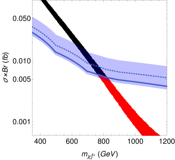
A number of different LHC searches can be used to set limits on the various particles of our example models. The simplest search, and currently the most stringent LHC limit for our models, comes from a recent ATLAS search for doubly charged particles decaying to either , or final states [26]. Results of our calculation, compared to the experimental limit are shown in fig. (7) for the final state.
The two-body decay with of the doubly charged scalar is approximately given by:
| (15) |
Since the Yukawa coupling does not enter the neutrino mass calculation, the exact value and flavour composition of this decay can not be predicted. However, enters our neutrino mass fit. The observed large neutrino angles require that all entries in the vector are different from zero and of similar order. Typically, from the fit we find numerically ratios in the range , but the exact ratios depend on the allowed range of neutrino angles. Scanning over the allowed neutrino parameters then leads to a variation of the branching ratios of the into the different lepton generations. This explains the spread of the numerically calculated points in fig. (7). Combined with the experimental limit from ATLAS, lower mass limits in the range of (600-800) GeV result. Note that in this plot, we allow all three neutrino angles to float within the 3 regions of the global fit [39].


The CMS collaboration has recently published a search based on multi-lepton final states [30]. The original motivation for this search is the expectation that the fermions of the seesaw type-III lead to final states containing multiple charged leptons and missing momentum. For example, from the associated production of the fermionic triplet . The analysis [30] requires than at least three charged leptons plus missing energy and takes into account both, electrons and muons.
In our models, these final states can occur in various decay chains. Consider for example . Once produced, it can decay into a , which further decays to a doubly charged scalar and . The doubly charged scalar decays to either leptons or ’s. The missing energy is then produced in the leptonic decays of the ’s. Here, all intermediate particles can be either on-shell or off-shell, depending on the unknown mass hierarchies. Constraints can then be derived from the results of [30], scanning over the allowed ranges of the branching ratios, which lead to a least three charged leptons plus at least one in the final state.
In fig. (8) we show results of this procedure for the examples of , and . The lower limits, derived from this exercise, have a rather large uncertainty, due to the unknown branching ratios. For example, the lower mass limit for is in the range of (550-850) GeV. Note that could decay, in principle to four charged leptons with a branching ratio close to 100 %. The final state from pair production of would then contain eight charged leptons and missing momentum would appear only from the decays of the ’s. In this case, our simple-minded recasting of the multi-lepton search [30] ceases to be valid and the lower limit on the mass of , mentioned above does not apply. As fig. (8) shows, the lower limit on the mass of is more stringent than the one for . This simply reflects the larger production cross sections for fermions, compare to fig. (6).
IV.2 New LNV searches
| Multiplicity | LNV Signal | Particles | Model | Mass range |
|---|---|---|---|---|
| 4 | , , | Q | TeV | |
| 6 | , | Q | TeV | |
| 6 | Q | TeV | ||
| 8 | - | - | ||
| 8 | Q | TeV | ||
| 8 | T | TeV |
We now turn to a discussion of possible LNV signals at the LHC. Table 1 shows examples of different LNV final states from pair production of scalars or fermions in the two models under consideration. This list is not complete since (a) associated producion of particles is not considered; (b) the table gives only “symmetric” LNV states, see below, and (c) we do not give LNV final states with neutrinos, since such states do not allow to establish LNV experimentally.
The table gives in column 1 the multiplicity of the final state and in column 2 the LNV signal. In that column, the two possible final states from the decay of the particle given in column 3 are given seperately. The invariant masses of both separate subsystems in column 2, should therefore give peaks in the mass of the particle in column 3.
Particles in column 3 are quoted as gauge eigenstates. However, scalars in our models are, in general, admixtures of different gauge eigenstates. Consider, for example, the simplest final state . can decay to , via the coupling , while can decay to via the induced vev (or, equivalently proportional to ). The doubly charged scalars mix via the entries in the mass matrices proportional to , (and ), see eq. (9). Whether the lightest doubly charged mass eigenstate is mostly , or depends on the choice of parameters, but the results are qualitatively very similar in all cases. We therefore show in fig. (9) only the results for the case where is mostly .


Fig. (9) (left) shows the ratio of branching ratios of the doubly charged scalar, decaying to divided by the decay to as a function of for some fixed choice of the other model parameters and three different values of . Observation of LNV is only possible, if is of similar order than , since both final states are needed to establish that LNV is indeed taking place. One can see from the figure that equality of partial widths is possible for different choices of parameters. However, since the decay to two charged leptons is proportional to (the square of) a Yukawa coupling that is not fixed by our neutrino mass fit, the relative ratio of branching ratios can not be predicted from current data.
Similarly, also for all other decays to LNV final states, the two competing final states have to have similar branching ratios. Fig. (9) to the right show results for the decay of of the triplet model. Depending on the parameter equality of branching ratio can occur in a large range of values of the parameter . Note that the rate of LNV final states is not suppressed by the smallness of neutrino masses. Neutrino masses require the product of to be small, see eq. (11). For a fixed neutrino mass, smaller values of require larger Yukawa couplings . Depending on the ratio between and , either the final state or the final state can dominate. Whether LNV rates are observable, therefore, does not depend so much on absolute values of some (supposedly small) parameters, but on certain ratios of these parameters.
Table 1 is ordered with respect to increasing multiplicity of the final state. Note that, as discussed in the last subsection, cross sections at the LHC increase with electric charge and decrease (strongly) with increasing mass. Which of the possible signals has the largest rate, can not be predicted because of the unknown mass spectrum. However, if the different members of the scalar (or fermion) multiplets have similar masses, final states with larger multiplicities have actually larger rates at the LHC. Since large multiplicity final states also have lower backgrounds, searches for such states should give stronger bounds.
The last column in table 1 gives our estimate for the reach of the LHC. The numbers for the mass reach quoted in that column are simply based on the cross section calculation, discussed in the last subsection. Since in particular for the high multiplicity final states we expect no SM backgrounds, we simply take the cross section for which 3 events for a luminosity of 300 are produced as the approximate limit, that maybe achieved in a dedicated search. In fact, with supposedly no backgrounds even slightly lower masses than those quoted in the table would lead to 5 or more events, sufficient for a discovery.
On the other hand, our calculation does not include any cuts and thus, should be taken only as a rough estimate. In particular, for the simpler signal , the number given in the table should be taken with a grain of salt. Currently for dilepton searches with luminosity of 36 there are no background events in the bins above TeV in the invariant mass distribution , see [26]. This in turns implies for a luminosity of 300 in the most pessimistic case an upper limit of roughly 8 background events for the signal . Our estimate of 3 signal events would then correspond only a 1 c.l. limit.
We mention that the final state with 2 and ’s and LNV signals with 10 or more particles are also possible in 1-loop models, but do not occur within our two example models. This is simply due to the fact that scalars or fermions with 5 units of charge are needed for such states. Thus, such signals can appear in versions of the 1-loop type models, that include larger representations, such as quintuplets, or with particles with a larger hypercharge.
Finally, the table considers only “symmetric” LNV final states. Here, by symmetric we define that both branches of the decay contain the same number of final states particles. For example, for the quadruplet model, we have included the LNV signal with ”symmetric” final states , but we have not considered the possible LNV signal with asymmetric final states . The reason for this choice is simply that we consider “asymmetric” LNV signals, although in principle possible, are less likely to occur. This can be understood simply from phase space considerations: A two-body final state has a prefactor of in the partial width, while a four-body phase space is smaller by a factor . Naturally one than expects that the ratio of branching ratios for these asymmetric cases is never close to one, unless there is a corresponding hierarchy in the couplings involved.
Decay widths for the lightest particle in our models are often very small numerically. This opens up the possibility that some particle decays might occur with a displaced vertex. Displaced vertices are more likely to occur in the triplet model, so we concentrate in our discussion on this case. The two-body decay width of is estimated in eq. (15). For the decay of , assuming is the lightest particle, one can estimate:
| (16) |
Here, is the mixing angle between the states and . Eq. (16) contains three parameters related to the smallness of the observed neutrino masses: , and . Assuming all mass parameters roughly equal this leads to the estimate:
| (17) |
Here, the choice for the Yukawa couplings being order is motivated by the upper limits on the CLFV branching ratios, discussed in the last section. Eq. (17) represents only a very rough estimate, but it is worth pointing out that more stringent upper limits from charged LFV would result in smaller values for the Yukawa couplings, leading to correspondingly large decay lengths. Note also that smaller values of would lead to quadratically large lengths. Eq. (17) shows that displaced vertices can occur easily in the decay of .
Similarly, one can estimate roughly the order of magnitude of the decay length for . The result is:
| (18) |
The width of is smaller than the corresponding one for due to the phase space suppression for a 4-body final state. Eq. (18) shows that within the triplet model a displaced vertex for the decay of is actually expected.
V Discussion and conclusions
In this paper we have discussed the phenomenology of 1-loop neutrino mass models. Models in this class are far from the simplest variants of BSM models that can fit existing neutrino data, but are interesting in their own right, since they predict that new physics must exist below roughly 2 TeV. If neutrino masses were indeed generated by one of the models in this class, one can thus expect that the LHC will find signatures of new resonances. Searches for doubly charged scalars and multi-lepton final states already put some bounds on these models. However, for the most interesting aspect of 1-loop models, namely lepton number violating final states, no LHC search exists so far. In particular, final states with large multiplicites are predicted to occur (multiple and multiple leptons) for which we expect standard model backgrounds to be negligible.
In our discussion, we have limited ourselves to just two simple example models. Our motivation to do so is that all 1-loop neutrino mass models, which are genuine in the sense that they give the leading contribution to neutrino mass without invoking new symmetries, predict similar LHC signals. The two models which we considered have either a triplet or a quadruplet as the largest representations. Other models will contain even larger multiplets and thus also particles with multiple electric charges, to which very similar constraints than those analysed here will apply.
Finally, we mention that there exist variants of 1-loop models, in which the internal scalars and fermions carry non-trivial colour charges. These variants are not fully covered by our analysis. While the neutrino mass fit and the constraints from LFV searches will be qualitatively very similar to what we have discussed here, additional color factors in the calculations will lead to some quantitative changes. The resulting bounds will, in general be somewhat more stringent than the numbers we give in this paper. More important, however, are the changes in the LHC phenomenology. For example, in the colour-singlet models, which we analyzed in this paper, the lightest doubly charged scalar will decay to two charged leptons. In the coloured variants of the model, the corresponding lightest scalar will behave like a leptoquark, decaying to , instead. Thus, different LHC searches will apply to the coloured models. More interesting, however, is that for coloured models also the LNV final states, which we discussed, will change, since at the end of the decay chain instead of two charged lepton, one lepton plus jet will appear. Although this variety of signals will be interesting in their own rights, we have concentraged here on the colour singlet variants of the model, because di-leptons are cleaner (and thus more easy to probe) in the challenging experimental environment that is the LHC.
Acknowledgements
This work was supported by the Spanish MICINN grants FPA2014-58183-P, FPU15/03158 (MECD) and PROMETEOII/2014/084 (Generalitat Valenciana). J.C.H. is supported by Chile grants Fondecyt No. 1161463, Conicyt PIA/ACT 1406 and Basal FB0821.
References
- [1] F. F. Deppisch, M. Hirsch, and H. Päs, J.Phys. G39, 124007 (2012), arXiv:1208.0727.
- [2] I. Avignone, Frank T., S. R. Elliott, and J. Engel, Rev.Mod.Phys. 80, 481 (2008), arXiv:0708.1033.
- [3] P. Minkowski, Phys.Lett. B67, 421 (1977).
- [4] T. Yanagida, Conf.Proc. C7902131, 95 (1979).
- [5] R. N. Mohapatra and G. Senjanovic, Phys. Rev. Lett. 44, 912 (1980).
- [6] Y. Cai, J. Herrero-García, M. A. Schmidt, A. Vicente, and R. R. Volkas, (2017), arXiv:1706.08524.
- [7] F. Bonnet, M. Hirsch, T. Ota, and W. Winter, JHEP 1207, 153 (2012), arXiv:1204.5862.
- [8] D. Aristizabal Sierra, A. Degee, L. Dorame, and M. Hirsch, JHEP 1503, 040 (2015), arXiv:1411.7038.
- [9] F. Bonnet, D. Hernandez, T. Ota, and W. Winter, JHEP 0910, 076 (2009), arXiv:0907.3143.
- [10] K. S. Babu, S. Nandi, and Z. Tavartkiladze, Phys. Rev. D80, 071702 (2009), arXiv:0905.2710.
- [11] R. Cepedello, M. Hirsch, and J. C. Helo, (2017), arXiv:1705.01489.
- [12] J. Helo, M. Hirsch, S. Kovalenko, and H. Päs, Phys.Rev. D88, 011901 (2013), arXiv:1303.0899.
- [13] J. Helo, M. Hirsch, H. Päs, and S. Kovalenko, Phys.Rev. D88, 073011 (2013), arXiv:1307.4849.
- [14] W.-Y. Keung and G. Senjanovic, Phys.Rev.Lett. 50, 1427 (1983).
- [15] CMS Collaboration, CMS-PAS-EXO-16-045 (2017).
- [16] CMS, V. Khachatryan et al., Eur. Phys. J. C74, 3149 (2014), arXiv:1407.3683.
- [17] CMS, A. M. Sirunyan et al., (2017), arXiv:1703.03995.
- [18] CMS, V. Khachatryan et al., JHEP 04, 169 (2016), arXiv:1603.02248.
- [19] ATLAS, G. Aad et al., JHEP 07, 162 (2015), arXiv:1506.06020.
- [20] J. Schechter and J. Valle, Phys. Rev. D22, 2227 (1980).
- [21] G. Azuelos, K. Benslama, and J. Ferland, J. Phys. G32, 73 (2006), arXiv:hep-ph/0503096.
- [22] P. Fileviez Perez, T. Han, G.-y. Huang, T. Li, and K. Wang, Phys. Rev. D78, 015018 (2008), arXiv:0805.3536.
- [23] A. Melfo, M. Nemevsek, F. Nesti, G. Senjanovic, and Y. Zhang, Phys. Rev. D85, 055018 (2012), arXiv:1108.4416.
- [24] ATLAS, G. Aad et al., JHEP 03, 041 (2015), arXiv:1412.0237.
- [25] ATLAS, ATLAS-CONF-2016-051 (2016).
- [26] ATLAS, ATLAS-CONF-2017-053 (2017).
- [27] CMS, CMS-PAS-HIG-14-039 (2016).
- [28] F. del Aguila, M. Chala, A. Santamaria, and J. Wudka, Phys. Lett. B725, 310 (2013), arXiv:1305.3904.
- [29] K. Ghosh, S. Jana, and S. Nandi, (2017), arXiv:1705.01121.
- [30] CMS, A. M. Sirunyan et al., (2017), arXiv:1708.07962.
- [31] S. Weinberg, Phys. Rev. Lett. 43, 1566 (1979).
- [32] E. Ma, Phys.Rev.Lett. 81, 1171 (1998), arXiv:hep-ph/9805219.
- [33] F. Staub, Comput.Phys.Commun. 184, pp. 1792 (2013), arXiv:1207.0906.
- [34] F. Staub, Comput.Phys.Commun. 185, 1773 (2014), arXiv:1309.7223.
- [35] F. Staub, T. Ohl, W. Porod, and C. Speckner, Comput.Phys.Commun. 183, 2165 (2012), arXiv:1109.5147.
- [36] W. Porod, Comput.Phys.Commun. 153, 275 (2003), arXiv:hep-ph/0301101.
- [37] W. Porod and F. Staub, Comput.Phys.Commun. 183, 2458 (2012), arXiv:1104.1573.
- [38] W. Porod, F. Staub, and A. Vicente, Eur. Phys. J. C74, 2992 (2014), arXiv:1405.1434.
- [39] D. Forero, M. Tortola, and J. Valle, Phys.Rev. D90, 093006 (2014), arXiv:1405.7540.
- [40] A. Vicente, Adv. High Energy Phys. 2015, 686572 (2015), arXiv:1503.08622.
- [41] MEG, A. M. Baldini et al., Eur. Phys. J. C76, 434 (2016), arXiv:1605.05081.
- [42] SINDRUM, U. Bellgardt et al., Nucl. Phys. B299, 1 (1988).
- [43] SINDRUM II, C. Dohmen et al., Phys. Lett. B317, 631 (1993).
- [44] A. M. Baldini et al., (2013), arXiv:1301.7225.
- [45] A. Blondel et al., (2013), arXiv:1301.6113.
- [46] The PRIME working group collaboration, S. Machida et al., (2003), LOI to JPARC, http://www-ps.kek.jp/jhf-np/LOIlist/pdf/L25.pdf.
- [47] Mu2e, G. Pezzullo, Nucl. Part. Phys. Proc. 285-286, 3 (2017), arXiv:1705.06461.
- [48] J. Alwall et al., JHEP 0709, 028 (2007), arXiv:0706.2334.
- [49] J. Alwall, M. Herquet, F. Maltoni, O. Mattelaer, and T. Stelzer, JHEP 1106, 128 (2011), arXiv:1106.0522.