跳到论文正文
W Papers独立论文阅读器 arXiv:1709.03116 论文正文 计算阅读时间 · 0%
引用这篇论文根据当前论文元数据生成,正式投稿前建议核对。


License: CC BY 4.0
arXiv:1709.03116v5 [math.GT] 07 Jul 2021

Computing twisted Alexander polynomials for Montesinos links

Haimiao Chen Note: Email: chenhm@math.pku.edu.cn Affiliation: Beijing Technology and Business University, Beijing, China
Abstract

In recent years, twisted Alexander polynomial has been playing an important role in low-dimensional topology. For Montesinos links, we develop an efficient method to compute the twisted Alexander polynomial associated to any linear representation. In particular, formulas for multi-variable Alexander polynomials of these links can be easily derived.

Keywords: linear representation, twisted Alexander polynomial, multi-variable Alexander polynomial, Montesinos link
MSC2020: 57K14

1 Introduction

Twisted Alexander polynomial (TAP for short) was first proposed by Lin [17] and Wada [24] independently. Given a link L⊂S3L\subset S^{3}. To each linear representation ρ\rho of π⁡(L):=π1​(S3−L)\pi(L):=\pi_{1}(S^{3}-L) is associated the TAP ΔL,ρ\Delta_{L,\rho}. People have found TAP to be extremely useful in low-dimensional topology.

Friedl and Vidussi [7] showed that TAP can detect the unknot and the Hopf link. They also constructed a pair of knots with the same HOMFLY polynomial, Khovanov and knot Floer homology, but distinguished by TAP.

As a classical result of Fox and Milnor [6], if KK is slice, then the ordinary Alexander polynomial can be written as f⁡(t)​f​(t−1)f(t)f(t^{-1}) for some ff. Generalized to TAP, more slice obstructions of such kind were obtained. Kirk and Livingston [14] showed that some knots (e.g. 8178_{17}) are not concordant to their inverses. Herald, Kirk and Livingston [11] showed that 16 of the knots with no more than 12 crossings are not slice; this could not be done before.

Fibredness can also be detected via TAP. Kitano and Morifuji [15] proved that if KK is fibered, then ΔK,ρ\Delta_{K,\rho} is monic of degree 4​g​(K)−24g(K)-2 (where g⁡(K)g(K) is the genus of KK) for any nonabelian ρ:π⁡(K)→SL⁡(2,𝔽)\rho:\pi(K)\to{\rm SL}(2,\mathbb{F}) for any field 𝔽\mathbb{F}. Closely related is the following

Conjecture 1.1 (Dunfield, Friedl and Jackson, 2012).

If KK is a hyperbolic knot and ρholo:π⁡(K)→SL⁡(2,ℂ)\rho_{\rm holo}:\pi(K)\to{\rm SL}(2,\mathbb{C}) is a lift of the discrete and faithful representation defining the hyperbolic metric, then deg⁡ΔK,ρholo=4​g​(K)−2\deg\Delta_{K,\rho_{\rm holo}}=4g(K)-2. Furthermore, KK is fibered if and only if ΔK,ρholo\Delta_{K,\rho_{\rm holo}} is monic.

The following result of Friedl and Vidussi [9] is remarkable: a knot KK is fibered if and only if there exist integers a,ba,b (which can be expressed in terms of invariants of KK) such that deg⁡ΔK,ρ=a​|G|+b\deg\Delta_{K,\rho}=a|G|+b for any representation ρ\rho factoring through a finite group GG.

Another topic attracting much attention is the relation K≥K′K\geq K^{\prime} defined by the existence of epimorphisms π⁡(K)↠π⁡(K′)\pi(K)\twoheadrightarrow\pi(K^{\prime}), which was known to be a partial order among prime knots. As shown in [16], if φ:π⁡(K)↠π⁡(K′)\varphi:\pi(K)\twoheadrightarrow\pi(K^{\prime}) is an epimorphism, then ΔK,ρ∘φ/ΔK′,ρ∈R⁡[t±1]\Delta_{K,\rho\circ\varphi}/\Delta_{K^{\prime},\rho}\in R[t^{\pm 1}] for any ρ:π⁡(K′)→GL⁡(d,R)\rho:\pi(K^{\prime})\to{\rm GL}(d,R).

For more applications of TAP, see [5, 8, 10, 12, 23] and the references therein.

TAP can be thought of as a non-abelian, yet manageable invariant. TAPs of twist knots for nonabelian SL⁡(2,ℂ){\rm SL}(2,\mathbb{C})-representations were computed in [18] and interesting applications were found. Hoste and Shanahan [13] computed ΔK,ρ\Delta_{K,\rho} for a class of 2-bridge knots KK and for ρ\rho factorizing through a dihedral group. Morifuji and Tran [19] computed TAPs associated to parabolic SL⁡(2,ℂ){\rm SL}(2,\mathbb{C})-representations of double twist knots and verified Conjecture 1.1. Tran [22] derived formulas for ΔK,ρ\Delta_{K,\rho}, when KK is a torus knot or a twist knot, and ρ\rho is the adjoint representation associated to an SL⁡(2,ℂ){\rm SL}(2,\mathbb{C})-representation. Besides these works, in the literature there are few computations for families of links or families of representations. Indeed, unlike the ordinary Alexander polynomial, in general there is no “skein relation” to use. For a link with mm crossings and a dd-dimensional linear representation, to obtain TAP by definition, one needs to compute the determinant of a matrix of size (m−1)​d×(m−1)​d(m-1)d\times(m-1)d, which is a tremendous job.

However, when restricted to Montesinos links LL, the situation is different. We shall develop an efficient method for deriving a “universal” formula for the TAP associated to any linear representation. For a dd-dimensional linear representation ρ\rho, we may reduce the computation of ΔL,ρ\Delta_{L,\rho} to those among d×dd\times d-matrices. This method will be useful for knot theorists to do computations. After all, Montesinos links, especially double twist links and pretzel links, are usually taken as examples to support general results, sometimes a new conjecture, as done in [1, 19, 20]. Specialized to the trivial representation, multi-variable Alexander polynomials are quickly computed, which will be beneficial to the realization problem of Alexander polynomials (see [21] Section 9). Furthermore, till now the relation ≥\geq between Montesinos knots is not well understood, neither is “1-domination” which is an enhance of ≥\geq (see [2]); we expect TAP to promote studying these relations.

The content is organized as follows. Section 2 is a preliminary, introducing some basic notions and recalling TAP. In Section 3 we present the method, and in Section 4 we give several practical examples for illustration.

Acknowledgement
This work is supported by NSFC-11401014, NSFC-11501014, NSFC-11771042.

2 Preliminary

Notation 2.1.

For a (not necessarily commutative) ring RR, let R×R^{\times} denote the set of invertible elements. For positive integers d,d′d,d^{\prime}, let ℳdd′​(R)\mathcal{M}^{d^{\prime}}_{d}(R) denote the set of d×d′d\times d^{\prime} matrices with entries in RR. Let ℳd​(R)=ℳdd​(R)\mathcal{M}_{d}(R)=\mathcal{M}^{d}_{d}(R).

Given A∈ℳdd′​(R)A\in\mathcal{M}^{d^{\prime}}_{d}(R). Let A¬i∈ℳd−1d′​(R)A_{\neg i}\in\mathcal{M}^{d^{\prime}}_{d-1}(R) (resp. A¬j∈ℳdd′−1​(R)A^{\neg j}\in\mathcal{M}^{d^{\prime}-1}_{d}(R)) be the matrix obtained by deleting the ii-th row (resp. jj-th column) of AA. For a ring homomorphism ψ:R→R′\psi:R\to R^{\prime} and A∈ℳdd′​(R)A\in\mathcal{M}^{d^{\prime}}_{d}(R), let ψ⁡(A)∈ℳdd′​(R′)\psi(A)\in\mathcal{M}^{d^{\prime}}_{d}(R^{\prime}) denote the matrix obtained from AA by replacing each entry with its image under ψ\psi.

For k∈ℤk\in\mathbb{Z} and a∈R×a\in R^{\times}, put

[k]a={1+a+⋯+ak−1,k>0,0,k=0,−ak​(1+a+⋯+a|k|−1),k<0.[k]_{a}=\begin{cases}1+a+\cdots+a^{k-1},&k>0,\\ 0,&k=0,\\ -a^{k}(1+a+\cdots+a^{|k|-1}),&k<0.\end{cases}

Given a group homomorphism σ:G→H\sigma:G\to H, let σˇ:ℤ​G→ℤ​H\check{\sigma}:\mathbb{Z}G\to\mathbb{Z}H denote the canonical linear extension, which is a ring homomorphism.

For two elements g,hg,h of a group, let g.h=g​h​g−1g.h=ghg^{-1}.

2.1 Twisted Alexander polynomial

Suppose LL is an oriented link with nn components. Take a planar diagram for LL. Numerating arbitrarily, let x1,…,xmx_{1},\ldots,x_{m} be the directed arcs, and κ1,…,κm\kappa_{1},\ldots,\kappa_{m} the crossings. Let FmF_{m} be the free group on the letters x~1,…,x~m\tilde{x}_{1},\ldots,\tilde{x}_{m}, with x~j\tilde{x}_{j} corresponding to xjx_{j}. With the “over presentation” (see [4] Chapter VI) for π=π1​(L)\pi=\pi_{1}(L), each positive crossing as in Figure 1 (a) gives rise to a relator x~j​x~k​x~j−1​x~ℓ−1\tilde{x}_{j}\tilde{x}_{k}\tilde{x}_{j}^{-1}\tilde{x}_{\ell}^{-1}, and each negative crossing as in Figure 1 (b) gives rise to a relator x~j−1​x~k​x~j​x~ℓ−1\tilde{x}_{j}^{-1}\tilde{x}_{k}\tilde{x}_{j}\tilde{x}_{\ell}^{-1}. By abuse of notation, we always denote the element of π\pi represented by a directed arc xx also by xx. Let ϕ:Fm↠π\phi:F_{m}\twoheadrightarrow\pi be the quotient map sending x~j\tilde{x}_{j} to xjx_{j}. Let M~∈ℳm​(ℤ​Fm)\widetilde{M}\in\mathcal{M}_{m}(\mathbb{Z}F_{m}) be the matrix whose (i,j)(i,j)-entry is ∂r~i/∂x~j\partial\tilde{r}_{i}/\partial\tilde{x}_{j} (the Fox derivative), and let M=ϕˇ​(M~)∈ℳm​(ℤ​π)M=\check{\phi}(\widetilde{M})\in\mathcal{M}_{m}(\mathbb{Z}\pi). Let

α:π↠H1​(S3−L)≅ℤn=⟨t1,…,tn⟩\alpha:\pi\twoheadrightarrow H_{1}(S^{3}-L)\cong\mathbb{Z}^{n}=\langle t_{1},\ldots,t_{n}\rangle

denote the abelianzation, with tkt_{k} the image of the kk-th meridian.

Refer to caption
Figure 1: (a) a positive crossing (xj,xk,xℓ)(x_{j},x_{k},x_{\ell}); (b) a negative crossing (xj,xk,xℓ)(x_{j},x_{k},x_{\ell})

Suppose RR is an integral domain. Let R⁡[𝐭±]=R⁡[t1±1,…,tn±1]R[\mathbf{t}^{\pm}]=R[t_{1}^{\pm 1},\ldots,t_{n}^{\pm 1}], and let R⁡(𝐭±)R(\mathbf{t}^{\pm}) denote its fraction field. For f1,f2∈R⁡(𝐭±)f_{1},f_{2}\in R(\mathbf{t}^{\pm}), denote f1≐f2f_{1}\doteq f_{2} if f2=ϵt1e1⋯tnenf1f_{2}=\epsilon t_{1}^{e_{1}}\cdots t_{n}^{e_{n}}f_{1} for some ϵ∈R×\epsilon\in R^{\times} and e1,…,en∈ℤe_{1},\ldots,e_{n}\in\mathbb{Z}; clearly ≐\doteq is an equivalence relation. Given a representation ρ:π→GL⁡(d,R)\rho:\pi\to{\rm GL}(d,R), the obvious map

π⟶α×ρℤn×GL⁡(d,R)↪R⁡[𝐭±1]×ℳd​(R)→ℳd​(R⁡[𝐭±])\pi\stackrel{{\scriptstyle\alpha\times\rho}}{{\longrightarrow}}\mathbb{Z}^{n}\times{\rm GL}(d,R)\hookrightarrow R[\mathbf{t}^{\pm 1}]\times\mathcal{M}_{d}(R)\to\mathcal{M}_{d}(R[\mathbf{t}^{\pm}])

can be extended by linearity to a ring homomorphism

ℤ​π→ℳd​(R⁡[𝐭±]),c↦c¯,\displaystyle\mathbb{Z}\pi\to\mathcal{M}_{d}(R[\mathbf{t}^{\pm}]),\qquad c\mapsto\overline{c}, (1)

Following [24], define the twisted Alexander polynomial by

ΔL,ρ≐det(M¬i¬j¯)det(1−xj¯)∈R⁡(𝐭±),\Delta_{L,\rho}\doteq\frac{\det\left(\overline{M_{\neg i}^{\neg j}}\right)}{\det(1-\overline{x_{j}})}\in R(\mathbf{t}^{\pm}),

with the understanding that, up to equivalence, the right-hand-side of ≐\doteq is independent of all the choices.

Let 𝟏\mathbf{1} denote the (1-dimensional) trivial representation. It is known that

ΔL,𝟏≐{ΔL/(t−1),n=1,ΔL,n≥2,\displaystyle\Delta_{L,\mathbf{1}}\doteq\begin{cases}\Delta_{L}/(t-1),&n=1,\\ \Delta_{L},&n\geq 2,\end{cases} (2)

where ΔL\Delta_{L} is the ordinary Alexander polynomial if n=1n=1, and is the multi-variable Alexander polynomial if n≥2n\geq 2.

2.2 Montesinos tangle and Montesinos link

Refer to caption
Figure 2: A tangle diagram with four ends
Refer to caption
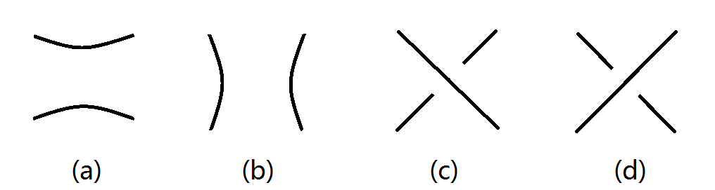
Figure 3: Four tangles in 𝒯22\mathcal{T}_{2}^{2}: (a) [0][0], (b) [∞][\infty], (c) [1][1], (d) [−1][-1]
Refer to caption
Figure 4: (a) T1+T2T_{1}+T_{2}; (b) T1∗T2T_{1}\ast T_{2}

Let 𝒯22\mathcal{T}_{2}^{2} denote the set of tangles TT with four ends Tnw,Tne,Tsw,TseT^{\rm nw},T^{\rm ne},T^{\rm sw},T^{\rm se}; see Figure 2. The simplest tangles in 𝒯22\mathcal{T}_{2}^{2} are shown in Figure 3. Defined on 𝒯22\mathcal{T}_{2}^{2} are horizontal composition ++ and vertical composition ∗\ast, as illustrated in Figure 4.

For k≠0k\neq 0, the horizontal composite of |k||k| copies of [1][1] (resp. [−1][-1]) is denoted by [k][k] if k>0k>0 (resp. k<0k<0), and the vertical composite of |k||k| copies of [1][1] (resp. [−1][-1]) is denoted by [1/k][1/k] if k>0k>0 (resp. k<0k<0). For k1,…,kr∈ℤk_{1},\ldots,k_{r}\in\mathbb{Z}, the rational tangle [[k1],…,[kr]][[k_{1}],\ldots,[k_{r}]] by definition is

{[k1]∗[1/k2]+⋯+[kr],if ​2∤r,[1/k1]+[k2]∗⋯+[kr],if ​2|r.\begin{cases}[k_{1}]\ast[1/k_{2}]+\cdots+[k_{r}],&\text{if\ \ }2\nmid r,\\ [1/k_{1}]+[k_{2}]\ast\cdots+[k_{r}],&\text{if\ \ }2\mid r.\end{cases}

Its fraction is given by the continued fraction [[k1,…,kr]]∈ℚ[[k_{1},\ldots,k_{r}]]\in\mathbb{Q}, which is defined inductively as

[[k1]]=k1;[[k1,…,kj]]=kj+1/[[k1,…,kj−1]],j≥2.[[k_{1}]]=k_{1};\qquad[[k_{1},\ldots,k_{j}]]=k_{j}+1/[[k_{1},\ldots,k_{j-1}]],\quad j\geq 2.

Denote [[k1],…,[kr]][[k_{1}],\ldots,[k_{r}]] as [p/q][p/q] when its fraction equals p/qp/q.

Refer to caption
Figure 5: (a) the numerator N⁡(T)N(T); (b) a tangle TT; (c) the denominator D⁡(T)D(T)

A Montesinos tangle is one of the form [p1/q1]∗⋯∗[pr/qr][p_{1}/q_{1}]\ast\cdots\ast[p_{r}/q_{r}].

Each T∈𝒯22T\in\mathcal{T}_{2}^{2} gives rise to two links: the numerator N⁡(T)N(T) and the denominator D⁡(T)D(T); see Figure 5. For p/q∈ℚp/q\in\mathbb{Q}, the link N⁡([p/q])N([p/q]) is called a rational link or 2-bridge link. In particular, N⁡([[k1],[k2]])N([[k_{1}],[k_{2}]]) is called a double twist link, and N⁡([[k1],[k2],[k3]])N([[k_{1}],[k_{2}],[k_{3}]]) is called a triple twist link. A link of the form D([p1/q1]∗⋯∗[ps/qs])D([p_{1}/q_{1}]\ast\cdots\ast[p_{s}/q_{s}]) is called a Montesinos link and denoted by M⁡(p1/q1,…,ps/qs)M(p_{1}/q_{1},\ldots,p_{s}/q_{s}); in particular, M⁡(p1,…,ps)M(p_{1},\ldots,p_{s}) is a pretzel link.

3 The method

The main results are (39) and (42), which are formulas of TAPs for rational links and general Montesinos links, respectively.

Notation 3.1.

For a crossing κi=(xj,xk,xℓ)\kappa_{i}=(x_{j},x_{k},x_{\ell}) as given in Figure 1, denote j,k,ℓj,k,\ell by i¯,i¯,i′\overline{i},\underline{i},i^{\prime}, respectively.

If κi\kappa_{i} is positive so that r~i=x~i¯​x~i¯​x~i¯−1​x~i′−1\tilde{r}_{i}=\tilde{x}_{\overline{i}}\tilde{x}_{\underline{i}}\tilde{x}_{\overline{i}}^{-1}\tilde{x}_{i^{\prime}}^{-1}, then

∂r~i∂x~i¯=1−x~i¯​x~i¯​x~i¯−1,∂r~i∂x~i¯=x~i¯,∂r~i∂x~i′=−x~i¯​x~i¯​x~i¯−1​x~i′−1,\frac{\partial\tilde{r}_{i}}{\partial\tilde{x}_{\overline{i}}}=1-\tilde{x}_{\overline{i}}\tilde{x}_{\underline{i}}\tilde{x}_{\overline{i}}^{-1},\qquad\frac{\partial\tilde{r}_{i}}{\partial\tilde{x}_{\underline{i}}}=\tilde{x}_{\overline{i}},\qquad\frac{\partial\tilde{r}_{i}}{\partial\tilde{x}_{i^{\prime}}}=-\tilde{x}_{\overline{i}}\tilde{x}_{\underline{i}}\tilde{x}_{\overline{i}}^{-1}\tilde{x}_{i^{\prime}}^{-1},

hence

ϕˇ​(∂r~i∂x~i¯)=1−xi′,ϕˇ​(∂r~i∂x~i¯)=xi¯,ϕˇ​(∂r~i∂x~i′)=−1,\check{\phi}\Big(\frac{\partial\tilde{r}_{i}}{\partial\tilde{x}_{\overline{i}}}\Big)=1-x_{i^{\prime}},\qquad\check{\phi}\Big(\frac{\partial\tilde{r}_{i}}{\partial\tilde{x}_{\underline{i}}}\Big)=x_{\overline{i}},\qquad\check{\phi}\Big(\frac{\partial\tilde{r}_{i}}{\partial\tilde{x}_{i^{\prime}}}\Big)=-1,

so that, written in matrices,

ϕˇ​[∂r~i∂x~i¯,∂r~i∂x~i¯,∂r~i∂x~i′]​D​[1−xi¯,1−xi¯,1−xi′]=(1−xi′)​[1−xi¯,xi¯,−1],\check{\phi}\left[\frac{\partial\tilde{r}_{i}}{\partial\tilde{x}_{\overline{i}}},\frac{\partial\tilde{r}_{i}}{\partial\tilde{x}_{\underline{i}}},\frac{\partial\tilde{r}_{i}}{\partial\tilde{x}_{i^{\prime}}}\right]D[1-x_{\overline{i}},1-x_{\underline{i}},1-x_{i^{\prime}}]=(1-x_{i^{\prime}})[1-x_{\overline{i}},x_{\overline{i}},-1],

where D⁡[a1,a2,a3]D[a_{1},a_{2},a_{3}] denotes the 3×33\times 3 diagonal matrix with diagonal entries aia_{i}.

If κi\kappa_{i} is negative so that r~i=x~i¯−1​x~i¯​x~i¯​x~i′−1\tilde{r}_{i}=\tilde{x}_{\overline{i}}^{-1}\tilde{x}_{\underline{i}}\tilde{x}_{\overline{i}}\tilde{x}_{i^{\prime}}^{-1}, then

∂r~i∂x~i¯=−x~i¯−1+x~i¯−1​x~i¯,∂r~i∂x~i¯=x~i¯−1,∂r~i∂x~i′=−x~i¯−1​x~i¯​x~i¯​x~i′−1,\frac{\partial\tilde{r}_{i}}{\partial\tilde{x}_{\overline{i}}}=-\tilde{x}_{\overline{i}}^{-1}+\tilde{x}_{\overline{i}}^{-1}\tilde{x}_{\underline{i}},\qquad\frac{\partial\tilde{r}_{i}}{\partial\tilde{x}_{\underline{i}}}=\tilde{x}_{\overline{i}}^{-1},\qquad\frac{\partial\tilde{r}_{i}}{\partial\tilde{x}_{i^{\prime}}}=-\tilde{x}_{\overline{i}}^{-1}\tilde{x}_{\underline{i}}\tilde{x}_{\overline{i}}\tilde{x}_{i^{\prime}}^{-1},

hence

ϕˇ​(∂r~i∂x~i¯)=−xi¯−1+xi′​xi¯−1,ϕˇ​(∂r~i∂x~i¯)=xi¯−1,ϕˇ​(∂r~i∂x~i′)=−1,\check{\phi}\Big(\frac{\partial\tilde{r}_{i}}{\partial\tilde{x}_{\overline{i}}}\Big)=-x_{\overline{i}}^{-1}+x_{i^{\prime}}x_{\overline{i}}^{-1},\qquad\check{\phi}\Big(\frac{\partial\tilde{r}_{i}}{\partial\tilde{x}_{\underline{i}}}\Big)=x_{\overline{i}}^{-1},\qquad\check{\phi}\Big(\frac{\partial\tilde{r}_{i}}{\partial\tilde{x}_{i^{\prime}}}\Big)=-1,

so that

ϕˇ​[∂r~i∂x~i¯,∂r~i∂x~i¯,∂r~i∂x~i′]​D​[1−xi¯,1−xi¯,1−xi′]=(1−xi′)​[1−xi¯−1,xi¯−1,−1].\check{\phi}\left[\frac{\partial\tilde{r}_{i}}{\partial\tilde{x}_{\overline{i}}},\frac{\partial\tilde{r}_{i}}{\partial\tilde{x}_{\underline{i}}},\frac{\partial\tilde{r}_{i}}{\partial\tilde{x}_{i^{\prime}}}\right]D[1-x_{\overline{i}},1-x_{\underline{i}},1-x_{i^{\prime}}]=(1-x_{i^{\prime}})[1-x_{\overline{i}}^{-1},x_{\overline{i}}^{-1},-1].

Consequently,

M​D=D′​Q,\displaystyle MD=D^{\prime}Q, (3)

where

  1. (i)

    D∈ℳm​(ℤ​π)D\in\mathcal{M}_{m}(\mathbb{Z}\pi) is diagonal, whose jj-th diagonal entry is 1−xj1-x_{j};

  2. (ii)

    D′∈ℳm​(ℤ​π)D^{\prime}\in\mathcal{M}_{m}(\mathbb{Z}\pi) is diagonal, whose ii-th diagonal entry is 1−xi′1-x_{i^{\prime}};

  3. (iii)

    Qi,i¯=1−xi¯ϵQ_{i,\overline{i}}=1-x_{\overline{i}}^{\epsilon}, Qi,i¯=xi¯ϵQ_{i,\underline{i}}=x_{\overline{i}}^{\epsilon}, Qi,i′=−1Q_{i,i^{\prime}}=-1, where ϵ=1\epsilon=1 (resp. ϵ=−1\epsilon=-1) if κi\kappa_{i} is positive (resp. negative), and Qi,j=0Q_{i,j}=0 for j∉{i¯,i¯,i′}j\notin\{\overline{i},\underline{i},i^{\prime}\}.

As a consequence of (3), for any i,ji,j, one has M¬i¬j​D¬j¬j=(D′)¬i¬i​Q¬i¬jM_{\neg i}^{\neg j}D_{\neg j}^{\neg j}=(D^{\prime})^{\neg i}_{\neg i}Q_{\neg i}^{\neg j}, so

ΔL,ρ≐det(M¬i¬j¯)det(1−xj¯)≐det(Q¬i¬j¯)det(1−xi′¯)≐det(Q¬i¬j¯)det(1−xi¯¯),\displaystyle\Delta_{L,\rho}\doteq\frac{\det\left(\overline{M_{\neg i}^{\neg j}}\right)}{\det(1-\overline{x_{j}})}\doteq\frac{\det\left(\overline{Q_{\neg i}^{\neg j}}\right)}{\det(1-\overline{x_{i^{\prime}}})}\doteq\frac{\det\left(\overline{Q_{\neg i}^{\neg j}}\right)}{\det(1-\overline{x_{\underline{i}}})}, (4)

the last equality following from that xi′x_{i^{\prime}} is conjugate to xi¯x_{\underline{i}}.

We shall do elementary transformations to convert QQ into another matrix which is highly simplified. To speak conveniently, introduce for each direct arc zz a formal variable ξz\xi_{z}. Each row of QQ corresponds to an equation ∑j=1mQi,j​ξxj=0,\sum_{j=1}^{m}Q_{i,j}\xi_{x_{j}}=0, and doing row-transformations is equivalent to re-writing equations of such kind. Note that ξz\xi_{z} depends only on the underlying arc of zz, so ξz′\xi_{z^{\prime}} also makes sense for an un-directed arc z′z^{\prime}.

Refer to caption
Figure 6: Four possibilities of a positive crossing
Refer to caption
Figure 7: Four possibilities of a negative crossing

For each crossing, let ξnw\xi_{\rm nw} denote the variable associated to the northwest arc, and so on. Adopt the following abbreviations:

ξ𝐰=[ξnwξsw],ξ𝐞=[ξneξse],ξ𝐧=[ξnwξne],ξ𝐬=[ξswξse].\xi_{\mathbf{w}}=\left[\begin{array}[]{cc}\xi_{\rm nw}\\ \xi_{\rm sw}\end{array}\right],\quad\xi_{\mathbf{e}}=\left[\begin{array}[]{cc}\xi_{\rm ne}\\ \xi_{\rm se}\end{array}\right],\quad\xi_{\mathbf{n}}=\left[\begin{array}[]{cc}\xi_{\rm nw}\\ \xi_{\rm ne}\end{array}\right],\quad\xi_{\mathbf{s}}=\left[\begin{array}[]{cc}\xi_{\rm sw}\\ \xi_{\rm se}\end{array}\right].

For a positive crossing shown in Figure 6, ξℓ=(1−xj)​ξj+xj​ξk\xi_{\ell}=(1-x_{j})\xi_{j}+x_{j}\xi_{k}, so in case (a), (b), (c), (d), respectively,

ξ𝐞=[1−xjxj10]​ξ𝐰,\displaystyle\xi_{\mathbf{e}}=\left[\begin{array}[]{cc}1-x_{j}&x_{j}\\ 1&0\end{array}\right]\xi_{\mathbf{w}}, ξ𝐬=[1−xj−1xj−110]​ξ𝐧,\displaystyle\xi_{\mathbf{s}}=\left[\begin{array}[]{cc}1-x_{j}^{-1}&x_{j}^{-1}\\ 1&0\end{array}\right]\xi_{\mathbf{n}},
ξ𝐞=[1−xj−1xj−110]​ξ𝐰,\displaystyle\xi_{\mathbf{e}}=\left[\begin{array}[]{cc}1-x_{j}^{-1}&x_{j}^{-1}\\ 1&0\end{array}\right]\xi_{\mathbf{w}}, ξ𝐬=[1−xjxj10]​ξ𝐧,\displaystyle\xi_{\mathbf{s}}=\left[\begin{array}[]{cc}1-x_{j}&x_{j}\\ 1&0\end{array}\right]\xi_{\mathbf{n}},
ξ𝐞=[01xj−11−xj−1]​ξ𝐰,\displaystyle\xi_{\mathbf{e}}=\left[\begin{array}[]{cc}0&1\\ x_{j}^{-1}&1-x_{j}^{-1}\end{array}\right]\xi_{\mathbf{w}}, ξ𝐬=[01xj−11−xj−1]​ξ𝐧,\displaystyle\xi_{\mathbf{s}}=\left[\begin{array}[]{cc}0&1\\ x_{j}^{-1}&1-x_{j}^{-1}\end{array}\right]\xi_{\mathbf{n}},
ξ𝐞=[01xj1−xj]​ξ𝐰,\displaystyle\xi_{\mathbf{e}}=\left[\begin{array}[]{cc}0&1\\ x_{j}&1-x_{j}\end{array}\right]\xi_{\mathbf{w}}, ξ𝐬=[01xj1−xj]​ξ𝐧.\displaystyle\xi_{\mathbf{s}}=\left[\begin{array}[]{cc}0&1\\ x_{j}&1-x_{j}\end{array}\right]\xi_{\mathbf{n}}.

For a negative crossing shown in Figure 7, ξℓ=(1−xj−1)​ξj+xj−1​ξk\xi_{\ell}=(1-x_{j}^{-1})\xi_{j}+x_{j}^{-1}\xi_{k}, so in case (a), (b), (c), (d), respectively,

ξ𝐞=[1−xj−1xj−110]​ξ𝐰,\displaystyle\xi_{\mathbf{e}}=\left[\begin{array}[]{cc}1-x_{j}^{-1}&x_{j}^{-1}\\ 1&0\end{array}\right]\xi_{\mathbf{w}}, ξ𝐬=[1−xjxj10]​ξ𝐧,\displaystyle\xi_{\mathbf{s}}=\left[\begin{array}[]{cc}1-x_{j}&x_{j}\\ 1&0\end{array}\right]\xi_{\mathbf{n}},
ξ𝐞=[1−xjxj10]​ξ𝐰,\displaystyle\xi_{\mathbf{e}}=\left[\begin{array}[]{cc}1-x_{j}&x_{j}\\ 1&0\end{array}\right]\xi_{\mathbf{w}}, ξ𝐬=[1−xj−1xj−110]​ξ𝐧,\displaystyle\xi_{\mathbf{s}}=\left[\begin{array}[]{cc}1-x_{j}^{-1}&x_{j}^{-1}\\ 1&0\end{array}\right]\xi_{\mathbf{n}},
ξ𝐞=[01xj1−xj]​ξ𝐰,\displaystyle\xi_{\mathbf{e}}=\left[\begin{array}[]{cc}0&1\\ x_{j}&1-x_{j}\end{array}\right]\xi_{\mathbf{w}}, ξ𝐬=[01xj1−xj]​ξ𝐧,\displaystyle\xi_{\mathbf{s}}=\left[\begin{array}[]{cc}0&1\\ x_{j}&1-x_{j}\end{array}\right]\xi_{\mathbf{n}},
ξ𝐞=[01xj−11−xj−1]​ξ𝐰,\displaystyle\xi_{\mathbf{e}}=\left[\begin{array}[]{cc}0&1\\ x_{j}^{-1}&1-x_{j}^{-1}\end{array}\right]\xi_{\mathbf{w}}, ξ𝐬=[01xj−11−xj−1]​ξ𝐧.\displaystyle\xi_{\mathbf{s}}=\left[\begin{array}[]{cc}0&1\\ x_{j}^{-1}&1-x_{j}^{-1}\end{array}\right]\xi_{\mathbf{n}}.
Notation 3.2.

For a rational tangle T=[[k1],…,[kr]]T=[[k_{1}],\ldots,[k_{r}]], introduce the “convenient labeling” for some of its directed arcs; see Figure 8.

Refer to caption
Figure 8: The “convenient labeling” of a rational tangle: (a) rr is odd; (b) rr is even

For k∈ℤk\in\mathbb{Z} and a,b∈πa,b\in\pi, put

uk​(a,b)\displaystyle u_{k}(a,b) ={[h]a​b​a​(1−b),k=2​h,[h+1]a​b​a−[h]a​b​a​b,k=2​h+1,\displaystyle=\begin{cases}[h]_{ab}a(1-b),&k=2h,\\ [h+1]_{ab}a-[h]_{ab}ab,&k=2h+1,\end{cases}
Gk​(a,b)\displaystyle G_{k}(a,b) =[1−uk​(a,b)uk​(a,b)1−uk−1​(a,b)uk−1​(a,b)].\displaystyle=\left[\begin{array}[]{cc}1-u_{k}(a,b)&u_{k}(a,b)\\ 1-u_{k-1}(a,b)&u_{k-1}(a,b)\\ \end{array}\right].

More explicitly,

G2​h​(a,b)\displaystyle G_{2h}(a,b) =[1−[h]a​b​(a−a​b)[h]a​b​(a−a​b)−[h]a​b​(a−1)1+[h]a​b​(a−1)],\displaystyle=\left[\begin{array}[]{cc}1-[h]_{ab}(a-ab)&[h]_{ab}(a-ab)\\ -[h]_{ab}(a-1)&1+[h]_{ab}(a-1)\\ \end{array}\right],
G2​h+1​(a,b)\displaystyle G_{2h+1}(a,b) =[−[h+1]a​b​(a−1)1+[h+1]a​b​(a−1)1−[h]a​b​(a−a​b)[h]a​b​(a−a​b)].\displaystyle=\left[\begin{array}[]{cc}-[h+1]_{ab}(a-1)&1+[h+1]_{ab}(a-1)\\ 1-[h]_{ab}(a-ab)&[h]_{ab}(a-ab)\\ \end{array}\right].

Using (3)–(3) iteratively, we obtain

[ξy(j)ξx(j)]=Gkj​(y(j−2),x(j−1))​[ξy(j−2)ξx(j−1)],\left[\begin{array}[]{cc}\xi_{y^{(j)}}\\ \xi_{x^{(j)}}\end{array}\right]=G_{k_{j}}(y^{(j-2)},x^{(j-1)})\left[\begin{array}[]{cc}\xi_{y^{(j-2)}}\\ \xi_{x^{(j-1)}}\end{array}\right],

The following is tautological:

Lemma 3.3.

Suppose T=[[k1],…,[kr]]T=[[k_{1}],\ldots,[k_{r}]]. Let ξ′=ξx(0),ξ′′=ξy(0)\xi^{\prime}=\xi_{x^{(0)}},\xi^{\prime\prime}=\xi_{y^{(0)}}. Then

ξTne=(1−bne)​ξ′+bne​ξ′′,ξTsw=(1−bsw)​ξ′+bsw​ξ′′,ξTse=(1−bse)​ξ′+bse​ξ′′,\xi_{T^{\rm ne}}=(1-b^{\rm ne})\xi^{\prime}+b^{\rm ne}\xi^{\prime\prime},\quad\xi_{T^{\rm sw}}=(1-b^{\rm sw})\xi^{\prime}+b^{\rm sw}\xi^{\prime\prime},\quad\xi_{T^{\rm se}}=(1-b^{\rm se})\xi^{\prime}+b^{\rm se}\xi^{\prime\prime},

with bne=ηy(r),bsw=ηy(r−1),bse=ηx(r)b^{\rm ne}=\eta_{y^{(r)}},b^{\rm sw}=\eta_{y^{(r-1)}},b^{\rm se}=\eta_{x^{(r)}}, where ηx(j),ηy(j)\eta_{x^{(j)}},\eta_{y^{(j)}} are recursively given by ηy(0)=1\eta_{y^{(0)}}=1, ηy(1)=uk1​(x(0),y(0))\eta_{y^{(1)}}=u_{k_{1}}(x^{(0)},y^{(0)}), ηx(1)=uk1−1​(x(0),y(0))\eta_{x^{(1)}}=u_{k_{1}-1}(x^{(0)},y^{(0)}), and

[ηy(j)ηx(j)]=Gkj​(y(j−2),x(j−1))​[ηy(j−2)ηx(j−1)],j≥2.\left[\begin{array}[]{cc}\eta_{y^{(j)}}\\ \eta_{x^{(j)}}\end{array}\right]=G_{k_{j}}(y^{(j-2)},x^{(j-1)})\left[\begin{array}[]{cc}\eta_{y^{(j-2)}}\\ \eta_{x^{(j-1)}}\end{array}\right],\qquad j\geq 2.

Suppose L=N⁡(T)L=N(T), with T=[[k1],…,[kr]]T=[[k_{1}],\ldots,[k_{r}]]. Let m=|k1|+⋯+|kr|m=|k_{1}|+\cdots+|k_{r}|. Define QT∈ℳmm+2​(ℤ​π)Q_{T}\in\mathcal{M}_{m}^{m+2}(\mathbb{Z}\pi) by setting each row to fit the condition (iii) following (3). Then each ξxj\xi_{x_{j}} can be written as (1−bj)​ξ′+bj​ξ′′(1-b_{j})\xi^{\prime}+b_{j}\xi^{\prime\prime} for some bj∈ℤ​πb_{j}\in\mathbb{Z}\pi. As effects on matrices, re-numbering columns beforehand if necessary, QTQ_{T} can be converted via a series of row transformations into

U​QT=[1−b1b1−1⋮⋮⋱1−bmbm−1],\displaystyle UQ_{T}=\left[\begin{array}[]{ccccc}1-b_{1}&b_{1}&-1&&\\ \vdots&\vdots&&\ddots&\\ 1-b_{m}&b_{m}&&&-1\\ \end{array}\right],

where bine=bne,bisw=bsw,bise=bseb_{i^{\rm ne}}=b^{\rm ne},b_{i^{\rm sw}}=b^{\rm sw},b_{i^{\rm se}}=b^{\rm se} for some ine,isw,ise∈{1,…,m}i^{\rm ne},i^{\rm sw},i^{\rm se}\in\{1,\ldots,m\}.

More precisely, as seen from (3)–(3), each of the row transformations used is or can be decomposed into special transformations, by which we mean those belong to the following:

  1. 1)

    multiplying the ii-th row by −xi′±1-x_{i^{\prime}}^{\pm 1}, for some ii;

  2. 2)

    adding (1−xi¯±1)(1-x_{\overline{i}}^{\pm 1}) times the ii-th row to or subtracting (1−xi¯±1)(1-x_{\overline{i}}^{\pm 1}) times the ii-th row from another row, for some ii.

Lemma 3.4.

Suppose f∈R⁡[𝐭±1]f\in R[\mathbf{t}^{\pm 1}], and suppose P∈GL⁡(m,ℤ​π)P\in{\rm GL}(m,\mathbb{Z}\pi) satisfies

det(P¬i¬j¯)≐det(1−xi′¯)​f\det\Big(\overline{P_{\neg i}^{\neg j}}\Big)\doteq\det(1-\overline{x_{i^{\prime}}})f

for all i,ji,j, then so does V​PVP, for any elementary matrix VV representing a special row transformation.

Proof.

It suffices to show that det((V​P)¬i¬j¯)\det\big(\overline{(VP)_{\neg i}^{\neg j}}\big) can be divided by det(1−xi′¯)​f\det(1-\overline{x_{i^{\prime}}})f, which can be verified directly. ∎

Note that U​QUQ can be obtained from U​QTUQ_{T} by deleting the columns corresponding to TneT^{\rm ne}, TseT^{\rm se}, and modifying the inei^{\rm ne}-th and isei^{\rm se}-th rows respectively according to ξTne=ξ′\xi_{T^{\rm ne}}=\xi^{\prime} and ξTse=ξTsw\xi_{T^{\rm se}}=\xi_{T^{\rm sw}}. Precisely, the inei^{\rm ne}-th row of U​QUQ is (−bne,bne,0,…,0)(-b^{\rm ne},b^{\rm ne},0,\ldots,0), and the isei^{\rm se}-th row is (bsw−bse,bse−bsw,0,…,0)(b^{\rm sw}-b^{\rm se},b^{\rm se}-b^{\rm sw},0,\ldots,0). This shows

det((U​Q)¬ise¬1¯)≐det(bne¯).\displaystyle\det\big(\overline{(UQ)_{\neg i^{\rm se}}^{\neg 1}}\big)\doteq\det\big(\overline{b^{\rm ne}}\big). (37)

We already know (retaining (4)) that det(Q¬i¬j¯)≐det(1−xi′¯)​ΔL,ρ\det\big(\overline{Q_{\neg i}^{\neg j}}\big)\doteq\det(1-\overline{x_{i^{\prime}}})\Delta_{L,\rho} for all i,ji,j, hence by Lemma 3.4,

det(Q¬ise¬1¯)≐det((U​Q)¬ise¬1¯)≐det(bne¯).\displaystyle\det\big(\overline{Q_{\neg i^{\rm se}}^{\neg 1}}\big)\doteq\det\big(\overline{(UQ)_{\neg i^{\rm se}}^{\neg 1}}\big)\doteq\det\big(\overline{b^{\rm ne}}\big). (38)

Thus by (4),

ΔN⁡(T),ρ≐det(bne¯)det(1−xse¯),\displaystyle\Delta_{N(T),\rho}\doteq\frac{\det\big(\overline{b^{\rm ne}}\big)}{\det(1-\overline{x^{\rm se}})}, (39)

where xsex^{\rm se} is the directed arc whose underlying arc is TseT^{\rm se}.

Now suppose L=D⁡(T)L=D(T), with T=T1∗⋯∗TsT=T_{1}\ast\cdots\ast T_{s}, (s≥2s\geq 2), each TkT_{k} being a rational tangle. Let mkm_{k} be the number of crossings in TkT_{k}, and let m=m1+⋯+msm=m_{1}+\cdots+m_{s}.

For each kk, similarly as above, set up QTkQ_{T_{k}} and bkneb_{k}^{\rm ne}, etc. Apply (1) to everything. To conveniently talk about row-transformations on QTk¯\overline{Q_{T_{k}}}, we introduce formal variables ξ¯xj,ξ¯k′,ξ¯k′′\overline{\xi}_{x_{j}},\overline{\xi}^{\prime}_{k},\overline{\xi}^{\prime\prime}_{k}, ξ¯Tkne\overline{\xi}_{T_{k}^{\rm ne}} and so on; abbreviate ξ¯Tkne\overline{\xi}_{T_{k}^{\rm ne}} to ξ¯kne\overline{\xi}_{k}^{\rm ne}, etc.

Suppose b1ne¯,…,bsne¯\overline{b_{1}^{\rm ne}},\ldots,\overline{b_{s}^{\rm ne}} are all invertible, i.e., det(bkne¯)≢0\det(\overline{b_{k}^{\rm ne}})\not\equiv 0 as elements of R⁡[𝐭±1]R[\mathbf{t}^{\pm 1}]. Re-write ξ¯kne=(1−bkne¯)​ξ¯k′+bkne¯​ξ¯k′′\overline{\xi}_{k}^{\rm ne}=(1-\overline{b_{k}^{\rm ne}})\overline{\xi}^{\prime}_{k}+\overline{b_{k}^{\rm ne}}\overline{\xi}^{\prime\prime}_{k} as

ξ¯k′′=(1−bkne¯−1)​ξ¯k′+bkne¯−1​ξ¯kne.\displaystyle\overline{\xi}^{\prime\prime}_{k}=(1-\overline{b_{k}^{\rm ne}}^{-1})\overline{\xi}^{\prime}_{k}+\overline{b_{k}^{\rm ne}}^{-1}\overline{\xi}_{k}^{\rm ne}. (40)

With ξ¯k′′\overline{\xi}^{\prime\prime}_{k} substituted, ξ¯xj\overline{\xi}_{x_{j}} for each xjx_{j} in TkT_{k} can be expressed as a linear combination of ξ¯k′\overline{\xi}^{\prime}_{k} and ξ¯kne\overline{\xi}_{k}^{\rm ne}; in particular,

[ξ¯kswξ¯kse]=[1−bksw¯​bkne¯−1bksw¯​bkne¯−11−bkse¯​bkne¯−1bkse¯​bkne¯−1]​[ξ¯k′ξ¯kne].\left[\begin{array}[]{cc}\overline{\xi}_{k}^{\rm sw}\\ \overline{\xi}_{k}^{\rm se}\end{array}\right]=\left[\begin{array}[]{cc}1-\overline{b_{k}^{\rm sw}}\overline{b_{k}^{\rm ne}}^{-1}&\overline{b_{k}^{\rm sw}}\overline{b_{k}^{\rm ne}}^{-1}\\ 1-\overline{b_{k}^{\rm se}}\overline{b_{k}^{\rm ne}}^{-1}&\overline{b_{k}^{\rm se}}\overline{b_{k}^{\rm ne}}^{-1}\end{array}\right]\left[\begin{array}[]{cc}\overline{\xi}^{\prime}_{k}\\ \overline{\xi}_{k}^{\rm ne}\end{array}\right].

The effect on QTk¯\overline{Q_{T_{k}}} is to multiply some U¯k∈GL⁡(mk,ℳ⁡(d,R⁡(𝐭±)))\overline{U}_{k}\in{\rm GL}(m_{k},\mathcal{M}(d,R(\mathbf{t}^{\pm}))) on the left. Note that det(U¯k)≐det(bkne¯)−1\det(\overline{U}_{k})\doteq\det(\overline{b_{k}^{\rm ne}})^{-1}, as we have multiplied bkne¯−1\overline{b_{k}^{\rm ne}}^{-1} to derive (40).

Since ξ¯k′=ξ¯k−1sw\overline{\xi}^{\prime}_{k}=\overline{\xi}_{k-1}^{\rm sw} and ξ¯kne=ξ¯k−1se\overline{\xi}_{k}^{\rm ne}=\overline{\xi}_{k-1}^{\rm se} for k=2,…,sk=2,\ldots,s, by further substituting, we can re-write each ξ¯xj\overline{\xi}_{x_{j}} as a linear combination of ξ¯1′\overline{\xi}^{\prime}_{1} and ξ¯1ne\overline{\xi}_{1}^{\rm ne}. What has been shown is that, re-numbering columns beforehand if necessary, we may take U¯∈GL⁡(m,ℳ⁡(d,R⁡(𝐭±)))\overline{U}\in{\rm GL}(m,\mathcal{M}(d,R(\mathbf{t}^{\pm}))) such that

det(U¯)≐∏k=1sdet(bkne¯)−1,U¯​Q¯=[⋆−I⁡(m−2)B−I⁡(2)].\det(\overline{U})\doteq\prod_{k=1}^{s}\det(\overline{b_{k}^{\rm ne}})^{-1},\qquad\overline{U}\overline{Q}=\left[\begin{array}[]{ccc}\star&-I(m-2)&\\ B&&-I(2)\end{array}\right].

The last two rows of U¯​Q¯\overline{U}\overline{Q} respectively express ξ¯ssw\overline{\xi}_{s}^{\rm sw} and ξ¯sse\overline{\xi}_{s}^{\rm se} as a linear combination of ξ¯1′\overline{\xi}^{\prime}_{1} and ξ¯1ne\overline{\xi}_{1}^{\rm ne}, i.e., [ξ¯sswξ¯sse]=B⁡[ξ¯1′ξ¯1ne]\left[\begin{array}[]{cc}\overline{\xi}_{s}^{\rm sw}\\ \overline{\xi}_{s}^{\rm se}\end{array}\right]=B\left[\begin{array}[]{cc}\overline{\xi}^{\prime}_{1}\\ \overline{\xi}_{1}^{\rm ne}\end{array}\right], with

B=[1−bssw¯​bsne¯−1bssw¯​bsne¯−11−bsse¯​bsne¯−1bsse¯​bsne¯−1]⋯[1−b1sw¯​b1ne¯−1b1sw¯​b1ne¯−11−b1se¯​b1ne¯−1b1se¯​b1ne¯−1]=[1−c¯c¯⋆⋆],B=\left[\begin{array}[]{cc}1-\overline{b_{s}^{\rm sw}}\overline{b_{s}^{\rm ne}}^{-1}&\overline{b_{s}^{\rm sw}}\overline{b_{s}^{\rm ne}}^{-1}\\ 1-\overline{b_{s}^{\rm se}}\overline{b_{s}^{\rm ne}}^{-1}&\overline{b_{s}^{\rm se}}\overline{b_{s}^{\rm ne}}^{-1}\end{array}\right]\cdots\left[\begin{array}[]{cc}1-\overline{b_{1}^{\rm sw}}\overline{b_{1}^{\rm ne}}^{-1}&\overline{b_{1}^{\rm sw}}\overline{b_{1}^{\rm ne}}^{-1}\\ 1-\overline{b_{1}^{\rm se}}\overline{b_{1}^{\rm ne}}^{-1}&\overline{b_{1}^{\rm se}}\overline{b_{1}^{\rm ne}}^{-1}\end{array}\right]=\left[\begin{array}[]{cc}1-\overline{c}&\overline{c}\\ \star&\star\end{array}\right],

where c¯=p¯1+p¯2q¯1+⋯+p¯sq¯s−1⋯q¯1\overline{c}=\overline{p}_{1}+\overline{p}_{2}\overline{q}_{1}+\cdots+\overline{p}_{s}\overline{q}_{s-1}\cdots\overline{q}_{1}, and

p¯k=bksw¯​bkne¯−1,q¯k=(bkse¯−bksw¯)​bkne¯−1.\overline{p}_{k}=\overline{b_{k}^{\rm sw}}\overline{b_{k}^{\rm ne}}^{-1},\qquad\overline{q}_{k}=(\overline{b_{k}^{\rm se}}-\overline{b_{k}^{\rm sw}})\overline{b_{k}^{\rm ne}}^{-1}.

Equating ξ¯ssw\overline{\xi}_{s}^{\rm sw}, ξ¯sse\overline{\xi}_{s}^{\rm se} with ξ¯1′\overline{\xi}^{\prime}_{1}, ξ¯1ne\overline{\xi}_{1}^{\rm ne}, respectively, similarly as (37), we obtain

det((U​Q)¬m¬1¯)≐det(c¯)⋅∏k=1sdet(bkne¯).\det(\overline{(UQ)_{\neg m}^{\neg 1}})\doteq\det(\overline{c})\cdot\prod\limits_{k=1}^{s}\det(\overline{b^{\rm ne}_{k}}).

Note that in above, each of row transformations other than multiplying via bkne¯−1\overline{b_{k}^{\rm ne}}^{-1} can be decomposed into special ones. Similarly as (38), by Lemma 3.4,

det(Q¬m¬1¯)≐det((U​Q)¬m¬1¯)≐det(c¯)⋅∏k=1sdet(bkne¯).\displaystyle\det(\overline{Q_{\neg m}^{\neg 1}})\doteq\det(\overline{(UQ)_{\neg m}^{\neg 1}})\doteq\det(\overline{c})\cdot\prod\limits_{k=1}^{s}\det(\overline{b^{\rm ne}_{k}}). (41)

Therefore, letting xssex_{s}^{\rm se} denote the directed arc whose underlying arc is TsseT_{s}^{\rm se},

ΔL,ρ≐∏k=1sdet(bkne¯)det(1−xsse¯)det(p¯1+p¯2q¯1+⋯+p¯sq¯s−1⋯q¯1).\displaystyle\Delta_{L,\rho}\doteq\frac{\prod_{k=1}^{s}\det(\overline{b^{\rm ne}_{k}})}{\det(1-\overline{x_{s}^{\rm se}})}\det(\overline{p}_{1}+\overline{p}_{2}\overline{q}_{1}+\cdots+\overline{p}_{s}\overline{q}_{s-1}\cdots\overline{q}_{1}). (42)

In particular, when s=3s=3,

ΔL,ρ≐det(b2ne¯)​det(b3ne¯)det(1−x3se¯)​det(b1sw¯+(b2sw¯+b3sw¯​b3ne¯−1​(b2se¯−b2sw¯))​b2ne¯−1​(b1se¯−b1sw¯)).\displaystyle\Delta_{L,\rho}\doteq\frac{\det(\overline{b_{2}^{\rm ne}})\det(\overline{b_{3}^{\rm ne}})}{\det(1-\overline{x_{3}^{\rm se}})}\det\Big(\overline{b_{1}^{\rm sw}}+\big(\overline{b_{2}^{\rm sw}}+\overline{b_{3}^{\rm sw}}\overline{b_{3}^{\rm ne}}^{-1}(\overline{b_{2}^{\rm se}}-\overline{b_{2}^{\rm sw}})\big)\overline{b_{2}^{\rm ne}}^{-1}(\overline{b_{1}^{\rm se}}-\overline{b_{1}^{\rm sw}})\Big). (43)

To deal with the “degenerate” case when det(bkne¯)≡0\det(\overline{b^{\rm ne}_{k}})\equiv 0 for some kk, we introduce auxiliary variables εk\varepsilon_{k} that commute with everything, replace bkne¯\overline{b^{\rm ne}_{k}} by bkne¯+εk​I\overline{b^{\rm ne}_{k}}+\varepsilon_{k}I, and run the process from (40) to (41). Then we arrive at

det(c¯′)⋅∏k=1sdet(bkne¯+εk​I),\displaystyle\det(\overline{c}^{\prime})\cdot\prod\limits_{k=1}^{s}\det(\overline{b^{\rm ne}_{k}}+\varepsilon_{k}I), (44)

(where c¯′\overline{c}^{\prime} is obtained from c¯\overline{c} via replacing bkne¯\overline{b^{\rm ne}_{k}} by bkne¯+εk​I\overline{b^{\rm ne}_{k}}+\varepsilon_{k}I), which can be expanded as a polynomial in ε1,…,εn\varepsilon_{1},\ldots,\varepsilon_{n}, since what is being computed is the determinant of some matrix whose entries are all such polynomials. Setting ε1=⋯=εn=0\varepsilon_{1}=\cdots=\varepsilon_{n}=0 in (44) and dividing by det(1−xsse¯)\det(1-\overline{x_{s}^{\rm se}}), we will obtain an expression for ΔL,ρ\Delta_{L,\rho}.

Remark 3.5.

We believe that each bkne¯\overline{b^{\rm ne}_{k}} is actually always invertible, but temporarily cannot prove this.

Remark 3.6.

Note that D(T1∗⋯∗Ts)D(T_{1}\ast\cdots\ast T_{s}) is the same as D(T2∗⋯∗Ts∗T1)D(T_{2}\ast\cdots\ast T_{s}\ast T_{1}), so the sub-indices in (42), (43) can be cyclically permuted.

In particular, if bisw=1b_{i}^{\rm sw}=1 for some i∈{1,2,3}i\in\{1,2,3\}, then with cyclical notations adopted, (43) can be simplified into

ΔL,ρ≐det(bi−1ne¯)det(1−xi−1se¯)​det(bi+1ne¯+(bise¯−1)​(bi+1sw¯+bi−1sw¯​bi−1ne¯−1​(bi+1se¯−bi+1sw¯))).\displaystyle\Delta_{L,\rho}\doteq\frac{\det(\overline{b_{i-1}^{\rm ne}})}{\det(1-\overline{x_{i-1}^{\rm se}})}\det\Big(\overline{b_{i+1}^{\rm ne}}+(\overline{b_{i}^{\rm se}}-1)\big(\overline{b_{i+1}^{\rm sw}}+\overline{b_{i-1}^{\rm sw}}\overline{b_{i-1}^{\rm ne}}^{-1}(\overline{b_{i+1}^{\rm se}}-\overline{b_{i+1}^{\rm sw}})\big)\Big). (45)

This will be useful in practical computations, as done in the next section.

4 Computations

Example 4.1.

Let KK be the triple twist knot N⁡([[2​h1],[2​h2],[2​h3+1]])N([[2h_{1}],[2h_{2}],[2h_{3}+1]]) given in Figure 9 (a). Apply Lemma 3.3 to compute ηy(0)=1\eta_{y^{(0)}}=1,

ηy(1)=u2​h1​(x,y)=[h1]x​y​(x−x​y),ηx(1)=u2​h1−1​(x,y)=w1+1,\displaystyle\eta_{y^{(1)}}=u_{2h_{1}}(x,y)=[h_{1}]_{xy}(x-xy),\qquad\eta_{x^{(1)}}=u_{2h_{1}-1}(x,y)=w_{1}+1,
[ηy(2)ηx(2)]=G2​h2​(y,x1−1)​[ηy(0)ηx(1)]=[1+[h2]y​x1−1​(y−y​x1−1)​w11+(w2+1)​w1],\displaystyle\left[\begin{array}[]{cc}\eta_{y^{(2)}}\\ \eta_{x^{(2)}}\end{array}\right]=G_{2h_{2}}(y,x_{1}^{-1})\left[\begin{array}[]{cc}\eta_{y^{(0)}}\\ \eta_{x^{(1)}}\end{array}\right]=\left[\begin{array}[]{cc}1+[h_{2}]_{yx_{1}^{-1}}(y-yx_{1}^{-1})w_{1}\\ 1+(w_{2}+1)w_{1}\end{array}\right],
[ηy(3)ηx(3)]=G2​h3+1​(y1,x2)​[ηy(1)ηx(2)]=[z⁡(w2​w1+(x​y)h1)+[h1]x​y​(x−x​y)⋆].\displaystyle\left[\begin{array}[]{cc}\eta_{y^{(3)}}\\ \eta_{x^{(3)}}\end{array}\right]=G_{2h_{3}+1}(y_{1},x_{2})\left[\begin{array}[]{cc}\eta_{y^{(1)}}\\ \eta_{x^{(2)}}\end{array}\right]=\left[\begin{array}[]{cc}z(w_{2}w_{1}+(xy)^{h_{1}})+[h_{1}]_{xy}(x-xy)\\ \star\\ \end{array}\right].

where

w1=[h1]x​y​(x−1),w2=[h2]y​x1−1​(y−1),z=[h3+1]y1​x2​y1−[h3]y1​x2​y1​x2,w_{1}=[h_{1}]_{xy}(x-1),\qquad w_{2}=[h_{2}]_{yx_{1}^{-1}}(y-1),\qquad z=[h_{3}+1]_{y_{1}x_{2}}y_{1}-[h_{3}]_{y_{1}x_{2}}y_{1}x_{2},

and ⋆\star denotes something irrelevant to us. By (39),

ΔL,ρ≐det(ηy3¯)det(1−xse¯)=det(z¯​(w2​w1¯+(x​y¯)h1)+[h1]x​y¯​(x¯−x​y¯))det(1−x¯)≐\displaystyle\Delta_{L,\rho}\doteq\frac{\det(\overline{\eta_{y_{3}}})}{\det(1-\overline{x^{\rm se}})}=\frac{\det(\overline{z}(\overline{w_{2}w_{1}}+(\overline{xy})^{h_{1}})+[h_{1}]_{\overline{xy}}(\overline{x}-\overline{xy}))}{\det(1-\overline{x})}\doteq
det(([h3+1]y1​x2¯​y1¯−[h3]y1​x2¯​y1​x2¯)​([h2]y¯​x1¯−1​(y¯−1)​[h1]x¯​y¯​(x¯−1)+(x¯​y¯)h1)+[h1]x¯​y¯​(x¯−x¯​y¯))det(1−x¯).\displaystyle\frac{\det\big(([h_{3}+1]_{\overline{y_{1}x_{2}}}\overline{y_{1}}-[h_{3}]_{\overline{y_{1}x_{2}}}\overline{y_{1}x_{2}})([h_{2}]_{\overline{y}\overline{x_{1}}^{-1}}(\overline{y}-1)[h_{1}]_{\overline{x}\overline{y}}(\overline{x}-1)+(\overline{x}\overline{y})^{h_{1}})+[h_{1}]_{\overline{x}\overline{y}}(\overline{x}-\overline{x}\overline{y})\big)}{\det(1-\overline{x})}.

In particular, when ρ=𝟏\rho=\mathbf{1} (the trivial representation), x¯=x1¯=x2¯=y¯=y1¯=t\overline{x}=\overline{x_{1}}=\overline{x_{2}}=\overline{y}=\overline{y_{1}}=t, and the ordinary Alexander polynomial is easily found (referring to (2)):

ΔK≐([h3+1]t2−t​[h3]t2)​(h2​(t−1)2​[h1]t2+t2​h1)+(1−t)​[h1]t2.\Delta_{K}\doteq([h_{3}+1]_{t^{2}}-t[h_{3}]_{t^{2}})(h_{2}(t-1)^{2}[h_{1}]_{t^{2}}+t^{2h_{1}})+(1-t)[h_{1}]_{t^{2}}.
Refer to caption
Figure 9: (a) The triple twist knot N⁡([[2​h1],[2​h2],[2​h3+1]])N([[2h_{1}],[2h_{2}],[2h_{3}+1]]); (b) The triple twist link N⁡([[2​h1],[2​h2],[2​h3]])N([[2h_{1}],[2h_{2}],[2h_{3}]])

As a special case, N⁡([2],[2],[3])N([2],[2],[3]) (with h1=h2=h3=1h_{1}=h_{2}=h_{3}=1) is the knot 757_{5}, so

Δ75,ρ≐det(y1¯​(1+x2​y1¯−x2¯)​(1−x¯−y¯+y¯​x¯+x¯​y¯)+x¯​(1−y¯))det(1−x¯).\displaystyle\Delta_{7_{5},\rho}\doteq\frac{\det\big(\overline{y_{1}}(1+\overline{x_{2}y_{1}}-\overline{x_{2}})(1-\overline{x}-\overline{y}+\overline{y}\overline{x}+\overline{x}\overline{y})+\overline{x}(1-\overline{y})\big)}{\det(1-\overline{x})}. (46)

In particular, the ordinary Alexander polynomial

Δ75≐2​t4−4​t3+5​t2−4​t+2.\Delta_{7_{5}}\doteq 2t^{4}-4t^{3}+5t^{2}-4t+2.

It is easy to see that π(75)=⟨x,y∣(x2y1)2=yx2y1x2⟩\pi(7_{5})=\langle x,y\mid(x_{2}y_{1})^{2}=yx_{2}y_{1}x_{2}\rangle, with y1=(x​y).xy_{1}=(xy).x, x2=(y​x).yx_{2}=(yx).y. Due to Δ75​(2)≡0(mod7)\Delta_{7_{5}}(2)\equiv 0\pmod{7}, there are homomorphisms

τϵ:π(75)→ℤ7⋊2ℤ3=⟨α,β∣α7=β3=1,βα=α2β⟩,ϵ∈{±1},\tau_{\epsilon}:\pi(7_{5})\to\mathbb{Z}_{7}\rtimes_{2}\mathbb{Z}_{3}=\langle\alpha,\beta\mid\alpha^{7}=\beta^{3}=1,\ \beta\alpha=\alpha^{2}\beta\rangle,\qquad\epsilon\in\{\pm 1\},

sending xx to βϵ\beta^{\epsilon} and yy to α​βϵ\alpha\beta^{\epsilon}. Let ζ=e2​π​i/7\zeta=e^{2\pi i/7}, and let ψ:ℤ7⋊2ℤ3→SL⁡(3,ℂ)\psi:\mathbb{Z}_{7}\rtimes_{2}\mathbb{Z}_{3}\to{\rm SL}(3,\mathbb{C}) denote the representation sending α,β\alpha,\beta to A,BA,B, respectively, where

A=[ζ000ζ2000ζ4],B=[010001100].A=\left[\begin{array}[]{ccc}\zeta&0&0\\ 0&\zeta^{2}&0\\ 0&0&\zeta^{4}\end{array}\right],\qquad B=\left[\begin{array}[]{ccc}0&1&0\\ 0&0&1\\ 1&0&0\end{array}\right].

Let ρϵ75:π⁡(75)→SL⁡(3,ℂ)\rho^{7_{5}}_{\epsilon}:\pi(7_{5})\to{\rm SL}(3,\mathbb{C}) be the composite ψ∘τϵ\psi\circ\tau_{\epsilon}. We can compute y1¯=t​A−2​ϵ​Bϵ\overline{y_{1}}=tA^{-2\epsilon}B^{\epsilon}, x2¯=t​A1+2​ϵ​Bϵ\overline{x_{2}}=tA^{1+2\epsilon}B^{\epsilon}, and then by (46),

Δ75,ρϵ75≐t9−5​t6+5​t3−1.\displaystyle\Delta_{7_{5},\rho^{7_{5}}_{\epsilon}}\doteq t^{9}-5t^{6}+5t^{3}-1. (47)
Example 4.2.

Let LL be the triple twist link N⁡([[2​h1],[2​h2],[2​h3]])N([[2h_{1}],[2h_{2}],[2h_{3}]]) given in Figure 9 (b). Similarly as in the previous Example,

ΔL,ρ≐det([h3]y1​x2¯​(y1¯−y1​x2¯)​(w2​w1¯+(x​y¯)h1)+[h1]x​y¯​(x¯−x​y¯))det(1−x3¯)≐\displaystyle\Delta_{L,\rho}\doteq\frac{\det([h_{3}]_{\overline{y_{1}x_{2}}}(\overline{y_{1}}-\overline{y_{1}x_{2}})(\overline{w_{2}w_{1}}+(\overline{xy})^{h_{1}})+[h_{1}]_{\overline{xy}}(\overline{x}-\overline{xy}))}{\det(1-\overline{x_{3}})}\doteq
det([h3]y1¯​x2¯​(y1¯−y1¯​x2¯)​([h2]y¯​x1¯−1​(y¯−1)​[h1]x¯​y¯​(x¯−1)+(x¯​y¯)h1)+[h1]x¯​y¯​(x¯−x¯​y¯))det(1−y¯).\displaystyle\frac{\det\big([h_{3}]_{\overline{y_{1}}\overline{x_{2}}}(\overline{y_{1}}-\overline{y_{1}}\overline{x_{2}})([h_{2}]_{\overline{y}\overline{x_{1}}^{-1}}(\overline{y}-1)[h_{1}]_{\overline{x}\overline{y}}(\overline{x}-1)+(\overline{x}\overline{y})^{h_{1}})+[h_{1}]_{\overline{x}\overline{y}}(\overline{x}-\overline{x}\overline{y})\big)}{\det(1-\overline{y})}.

The multi-variable Alexander polynomial can be easily found by setting x¯=y1¯=t1\overline{x}=\overline{y_{1}}=t_{1} and y¯=x1¯=x2¯=t2\overline{y}=\overline{x_{1}}=\overline{x_{2}}=t_{2}:

OPENΔL≐[h1]t1​t2​[h3]t1​t2​(h2​(t1−1)​(t2−1)+t1​t2−1)+[h1]t1​t2+[h3]t1​t2).\Delta_{L}\doteq[h_{1}]_{t_{1}t_{2}}[h_{3}]_{t_{1}t_{2}}(h_{2}(t_{1}-1)(t_{2}-1)+t_{1}t_{2}-1)+[h_{1}]_{t_{1}t_{2}}+[h_{3}]_{t_{1}t_{2}}).
Example 4.3.
Refer to caption
Figure 10: The pretzel knot P⁡(2​k1+1,2​k2+1,2​k3+1)P(2k_{1}+1,2k_{2}+1,2k_{3}+1)

Let K=P⁡(2​k1+1,2​k2+1,2​k3+1)K=P(2k_{1}+1,2k_{2}+1,2k_{3}+1). It is easy to see that

b1se=u2​k1​(x2,x3−1),b2se=u2​k2​(x3,x1−1),b2ne=u2​k2+1​(x3,x1−1),b_{1}^{\rm se}=u_{2k_{1}}(x_{2},x_{3}^{-1}),\qquad b_{2}^{\rm se}=u_{2k_{2}}(x_{3},x_{1}^{-1}),\qquad b_{2}^{\rm ne}=u_{2k_{2}+1}(x_{3},x_{1}^{-1}),

and bisw=1b_{i}^{\rm sw}=1, i=1,2,3i=1,2,3. Let

zi=[ki]xi+1​xi−1−1​xi+1​(1−xi−1−1)−1,wi=[ki+1]xi+1​xi−1−1​(xi+1−1)+1.z_{i}=[k_{i}]_{x_{i+1}x_{i-1}^{-1}}x_{i+1}(1-x_{i-1}^{-1})-1,\qquad w_{i}=[k_{i}+1]_{x_{i+1}x_{i-1}^{-1}}(x_{i+1}-1)+1.

Then by (45),

ΔK,ρ≐det(w3¯)det(1−x1¯)​det(w2¯+z1¯​(1+w3¯−1​z2¯)).\displaystyle\Delta_{K,\rho}\doteq\frac{\det(\overline{w_{3}})}{\det(1-\overline{x_{1}})}\det\big(\overline{w_{2}}+\overline{z_{1}}(1+\overline{w_{3}}^{-1}\overline{z_{2}})\big). (48)

In particular, the ordinary Alexander polynomial is

ΔK≐1+(1+k1+k2+k3+k1​k2+k2​k3+k1​k3)​(t+t−1−2).\Delta_{K}\doteq 1+(1+k_{1}+k_{2}+k_{3}+k_{1}k_{2}+k_{2}k_{3}+k_{1}k_{3})(t+t^{-1}-2).

Consider the case k1=k2=k3=1k_{1}=k_{2}=k_{3}=1. We have

z1¯\displaystyle\overline{z_{1}} =t​ρ​(x2)−ρ⁡(x2​x3−1)−1,\displaystyle=t\rho(x_{2})-\rho(x_{2}x_{3}^{-1})-1, (49)
z2¯\displaystyle\overline{z_{2}} =t​ρ​(x3)+t​ρ​(x3​x1−1)−1,\displaystyle=t\rho(x_{3})+t\rho(x_{3}x_{1}^{-1})-1, (50)
w2¯\displaystyle\overline{w_{2}} =t​ρ​(x3)+t​ρ​(x3​x1−1​x3)+ρ⁡(x3​x1−1),\displaystyle=t\rho(x_{3})+t\rho(x_{3}x_{1}^{-1}x_{3})+\rho(x_{3}x_{1}^{-1}), (51)
w3¯\displaystyle\overline{w_{3}} =t​ρ​(x1)+t​ρ​(x1​x2−1​x1)−ρ⁡(x1​x2−1).\displaystyle=t\rho(x_{1})+t\rho(x_{1}x_{2}^{-1}x_{1})-\rho(x_{1}x_{2}^{-1}). (52)

The results of [3] enable us to easily construct irreducible 2-dimensional representations of π⁡(K)\pi(K). For instance, the assignment

x1↦[1101],x2↦[10−31],x3↦[21−10]x_{1}\mapsto\left[\begin{array}[]{cc}1&1\\ 0&1\end{array}\right],\qquad x_{2}\mapsto\left[\begin{array}[]{cc}1&0\\ -3&1\end{array}\right],\qquad x_{3}\mapsto\left[\begin{array}[]{cc}2&1\\ -1&0\end{array}\right]

defines a representation ρ:π⁡(K)→SL⁡(2,𝔽11)\rho:\pi(K)\to{\rm SL}(2,\mathbb{F}_{11}), as can be checked using (16)–(18) of [3]. By (48) and (49)–(52), we can compute

ΔP⁡(3,3,3),ρ≐(t+2)​(t+4)​(t2+3​t−2)(t−1)2∈𝔽11​(t).\Delta_{P(3,3,3),\rho}\doteq\frac{(t+2)(t+4)(t^{2}+3t-2)}{(t-1)^{2}}\in\mathbb{F}_{11}(t).
Example 4.4.

Let LL be the 3-component pretzel link P⁡(2​k1,2​k2,2​k3)P(2k_{1},2k_{2},2k_{3}).

Refer to caption
Figure 11: The pretzel link P⁡(2​k1,2​k2,2​k3)P(2k_{1},2k_{2},2k_{3})

For i=1,2,3i=1,2,3, let yi=xi+1​xi−1−1y_{i}=x_{i+1}x_{i-1}^{-1}, and vi=[ki]yiv_{i}=[k_{i}]_{y_{i}}, then bisw=1b_{i}^{\rm sw}=1, bine=vi​(xi+1−yi)b_{i}^{\rm ne}=v_{i}(x_{i+1}-y_{i}), bise=vi​(xi+1−1)+1b_{i}^{\rm se}=v_{i}(x_{i+1}-1)+1. By (45),

ΔL,ρ≐det(v3¯​(x1¯−y3¯))det(1−x2¯)​det(v2¯​(x3¯−y2¯)+v1¯​(x2¯−1)+v1¯​(v3¯​y3¯)−1​v2¯​(x3¯−1)).\Delta_{L,\rho}\doteq\frac{\det(\overline{v_{3}}(\overline{x_{1}}-\overline{y_{3}}))}{\det(1-\overline{x_{2}})}\det\Big(\overline{v_{2}}(\overline{x_{3}}-\overline{y_{2}})+\overline{v_{1}}(\overline{x_{2}}-1)+\overline{v_{1}}(\overline{v_{3}}\overline{y_{3}})^{-1}\overline{v_{2}}(\overline{x_{3}}-1)\Big).

Specialized to ρ=𝟏\rho=\mathbf{1} so that xi¯=ti\overline{x_{i}}=t_{i}, the multi-variable Alexander polynomial is easily found:

ΔL≐∑i=13ti−1​(ti−1)​[ki+1]ti−1​ti−1​[ki−1]ti​ti+1−1.\Delta_{L}\doteq\sum\limits_{i=1}^{3}t_{i-1}(t_{i}-1)[k_{i+1}]_{t_{i-1}t_{i}^{-1}}[k_{i-1}]_{t_{i}t_{i+1}^{-1}}.

As a special case when k1=k2=k3=1k_{1}=k_{2}=k_{3}=1, L=P⁡(2,2,2)L=P(2,2,2) is the 3-chain link, a very interesting link whose complement in S3S^{3} is named the “magic manifold”. The formula can be simplified into

ΔP⁡(2,2,2),ρ≐det((x2¯−1+x1¯−1)​(x3¯−1)−x2¯−1​x3¯​x1¯−1+1).\Delta_{P(2,2,2),\rho}\doteq\det((\overline{x_{2}}^{-1}+\overline{x_{1}}^{-1})(\overline{x_{3}}-1)-\overline{x_{2}}^{-1}\overline{x_{3}}\overline{x_{1}}^{-1}+1).
Example 4.5.

Let K=M⁡(7/3,2,7/2)K=M(7/3,2,7/2), which is the mirror of 12​a​_​042312a\_0423 in the knot table. Write K=D⁡(T1∗T2∗T3)K=D(T_{1}\ast T_{2}\ast T_{3}), with T1=[[3],[2]]T_{1}=[[3],[2]], T2=[2]T_{2}=[2], T3=[[2],[3]]T_{3}=[[2],[3]]. Use x,y,zx,y,z to express other elements:

x′=z−1.x,y′=(x​y−1​x).y,z′=(x​z)−1.z,w=(x​y−1).x.\displaystyle x^{\prime}=z^{-1}.x,\qquad y^{\prime}=(xy^{-1}x).y,\qquad z^{\prime}=(xz)^{-1}.z,\qquad w=(xy^{-1}).x.
Refer to caption
Figure 12: The knot M⁡(7/3,2,7/2)M(7/3,2,7/2)

Computing routinely,

b1sw\displaystyle b_{1}^{\rm sw} =u3​(x,y−1)=x⁡(1+y−1​x−y−1),\displaystyle=u_{3}(x,y^{-1})=x(1+y^{-1}x-y^{-1}),
[b1neb1se]\displaystyle\left[\begin{array}[]{cc}b_{1}^{\rm ne}\\ b_{1}^{\rm se}\end{array}\right] =G2​(y−1,w−1)​[1u2​(x,y−1)]=[1+y−1​(1−w−1)​(x−x​y−1−1)⋆],\displaystyle=G_{2}(y^{-1},w^{-1})\left[\begin{array}[]{cc}1\\ u_{2}(x,y^{-1})\end{array}\right]=\left[\begin{array}[]{cc}1+y^{-1}(1-w^{-1})(x-xy^{-1}-1)\\ \star\end{array}\right],
b2se\displaystyle b_{2}^{\rm se} =y′,\displaystyle=y^{\prime},
b3sw\displaystyle b_{3}^{\rm sw} =u2​(x′,z′)=x′​(1−z′),\displaystyle=u_{2}(x^{\prime},z^{\prime})=x^{\prime}(1-z^{\prime}),
[b3neb3se]\displaystyle\left[\begin{array}[]{cc}b_{3}^{\rm ne}\\ b_{3}^{\rm se}\end{array}\right] =G3​(z′,z−1)​[1x′]=[1+z′​(1+z−1​z′−z−1)​(x′−1)1+z′​(1−z−1)​(x′−1)].\displaystyle=G_{3}(z^{\prime},z^{-1})\left[\begin{array}[]{cc}1\\ x^{\prime}\end{array}\right]=\left[\begin{array}[]{cc}1+z^{\prime}(1+z^{-1}z^{\prime}-z^{-1})(x^{\prime}-1)\\ 1+z^{\prime}(1-z^{-1})(x^{\prime}-1)\end{array}\right].

Then ΔK,ρ\Delta_{K,\rho} can be obtained via (45) by plugging in these.

Specialized to ρ=𝟏\rho=\mathbf{1},

b1sw¯=2​t−1,b2se¯=t,b3sw¯=t−t2,t2​b1ne¯=b3ne¯=b3se¯−b3sw¯=2​t2−3​t+2,\overline{b_{1}^{\rm sw}}=2t-1,\quad\overline{b_{2}^{\rm se}}=t,\quad\overline{b_{3}^{\rm sw}}=t-t^{2},\qquad t^{2}\overline{b_{1}^{\rm ne}}=\overline{b_{3}^{\rm ne}}=\overline{b_{3}^{\rm se}}-\overline{b_{3}^{\rm sw}}=2t^{2}-3t+2,

leading us to

ΔK≐(2​t2−3​t+2)​(2​t4−4​t3+5​t2−4​t+2)≐(2​t2−3​t+2)​Δ75.\Delta_{K}\doteq(2t^{2}-3t+2)(2t^{4}-4t^{3}+5t^{2}-4t+2)\doteq(2t^{2}-3t+2)\Delta_{7_{5}}.

Similarly as in Example 4.1, we can consider representations π⁡(K)→ℤ7⋊2ℤ3\pi(K)\to\mathbb{Z}_{7}\rtimes_{2}\mathbb{Z}_{3}. The relations of π⁡(K)\pi(K) are

(w​y)−1.y=(z′​z−1).z′,y−1.w=(y′​x′).y′,(wy)^{-1}.y=(z^{\prime}z^{-1}).z^{\prime},\qquad y^{-1}.w=(y^{\prime}x^{\prime}).y^{\prime},

from which it follows that the assignment x↦βx\mapsto\beta, y↦αa​βy\mapsto\alpha^{a}\beta, z↦αb​βz\mapsto\alpha^{b}\beta defines a nonabelian representation π⁡(K)→ℤ7⋊2ℤ3\pi(K)\to\mathbb{Z}_{7}\rtimes_{2}\mathbb{Z}_{3} if and only if b≡a≢0(mod7)b\equiv a\not\equiv 0\pmod{7}. Let ρaK:π⁡(K)→SL⁡(3,ℂ)\rho^{K}_{a}:\pi(K)\to{\rm SL}(3,\mathbb{C}) denote the composite of this representation with ψ\psi (given in Example 4.1). With the help of Mathematica, we compute

ΔK,ρaK≐\displaystyle\Delta_{K,\rho^{K}_{a}}\doteq 1t3−1​(t18−(2​ζ5​a+3​ζ4​a+ζ3​a+4​ζ2​a+3​ζa+5)​t15+(11​ζ5​a+2​ζ4​aCLOSECLOSE\displaystyle\ \frac{1}{t^{3}-1}\Big(t^{18}-(2\zeta^{5a}+3\zeta^{4a}+\zeta^{3a}+4\zeta^{2a}+3\zeta^{a}+5)t^{15}+(11\zeta^{5a}+2\zeta^{4a}
OPEN+10​ζ3​a+10​ζ2​a+7​ζa+8)​t12−(4​ζ5​a+3​ζ4​a+8​ζ3​a+6​ζ2​a−ζa)​t9−\displaystyle+10\zeta^{3a}+10\zeta^{2a}+7\zeta^{a}+8)t^{12}-(4\zeta^{5a}+3\zeta^{4a}+8\zeta^{3a}+6\zeta^{2a}-\zeta^{a})t^{9}-
OPEN(4​ζ5​a+ζ3​a+5​ζ2​a+3​ζa+9)​t6+(ζ5​a+2​ζ3​a+3​ζ2​a+2​ζa+2)​t3+1).\displaystyle(4\zeta^{5a}+\zeta^{3a}+5\zeta^{2a}+3\zeta^{a}+9)t^{6}+(\zeta^{5a}+2\zeta^{3a}+3\zeta^{2a}+2\zeta^{a}+2)t^{3}+1\Big).

Assume there exists an epimorphism ϕ:π⁡(K)↠π⁡(75)\phi:\pi(K)\twoheadrightarrow\pi(7_{5}). Then ρε75∘ϕ\rho^{7_{5}}_{\varepsilon}\circ\phi is conjugate to ρaK\rho^{K}_{a} for some aa and ε∈{±1}\varepsilon\in\{\pm 1\}. However, looking back to (47), we see that Δ75,ρ±175∤ΔK,ρaK\Delta_{7_{5},\rho^{7_{5}}_{\pm 1}}\nmid\Delta_{K,\rho^{K}_{a}}. Thus, while the ordinary Alexander polynomial does not detect K⩾̸75K\ngeqslant 7_{5}, TAP does.

References

  • [1] A. Aso, Twisted Alexander polynomials of (−2,3,2​n+1)(-2,3,2n+1)-pretzel knots, arXiv: 1803.06470.
  • [2] M. Boileau, S. Boyer, D. Rolfsen, S.-C. Wang, 1-domination of knots, Illinois J. Math. 60 (2016), no. 1, 117–139.
  • [3] H.-M. Chen, Character varieties of odd classical pretzel knots, Int. J. Math. 29 (2018), no. 9, 1850060 (15 pages).
  • [4] R.H. Crowell, R. Fox, Introduction to knot theory. Graduate Texts in Mathematics 57, Springer-Verlag, New York, Heidelberg, Berlin, 1977.
  • [5] J. Dubois, S. Friedl, W. Lück, Three flavors of twisted invariants of knots, (English summary) Introduction to modern mathematics, 143–169, Adv. Lect. Math. (ALM), 33, Int. Press, Somerville, MA, 2015.
  • [6] R.H. Fox, J.W. Milnor, Singularities of 2-spheres in 4-space and cobordism of knots, Osaka J. Math. 3 (1966), 257–267.
  • [7] S. Friedl, S. Vidussi, Nontrivial Alexander polynomials of knots and links, Bull. Lond. Math. Soc. 39 (2007), 614–622.
  • [8] S. Friedl, S. Vidussi, A survey of twisted Alexander polynomials, Proceedings of the conference ‘The mathematics of knots: theory and application’, Heidelberg, December, 2008.
  • [9] S. Friedl, S. Vidussi, Twisted Alexander polynomials detect fibered 3-manifolds, Ann. Math. 173 (2011), 1587–1643.
  • [10] H. Goda, Twisted Alexander invariants and hyperbolic volume, Proc. Japan Acad. Ser. A 93 (2017), no. 7, 61–66.
  • [11] C. Herald, P. Kirk, C. Livingston, Metabelian representations, twisted Alexander polynomials, knot slicing, and mutation, Math. Z. 265 (2010), no. 4, 925–949.
  • [12] J.A. Hillman, C. Livinston, S. Naik, Twisted Alexander polynomials of periodic knots, Algebr. Geom. Topol. 6 (2006), 145–169.
  • [13] J. Hoste, P.D. Shanahan, Twisted Alexander polynomials of 2-bridge knots, J. Knot Theor. Ramif. 22 (2013), no. 1, 1250138 (29 pages).
  • [14] P. Kirk, C. Livingston, Twisted knot polynomials: inversion, mutation and concordance, Topology 38 (1999), no. 3, 663–671.
  • [15] T. Kitano, T. Morifuji, Divisibility of twisted Alexander polynomials and fibered knots, Ann. Scuola Norm. Sup. Pisa CI. Sci. (5) 4 (2005), 179–186.
  • [16] T. Kitano, M. Suzuki, M. Wada, Twisted Alexander polynomials and surjectivity of a group homomorphism, Algebr. Geom. Topol. 5 (2005), 1315–1324.
  • [17] X.-S. Lin, Representations of knot groups and twisted Alexander polynomials, Acta Math. Sin (Engl. Ser.) 17 (2001), 361–380.
  • [18] T. Morifuji, Twisted Alexander polynomials of twist knots for nonabelian representations, Bull. Sci. Math. 132 (2008), 439–453.
  • [19] T. Morifuji, A.T. Tran, Twisted Alexander polynomial of 2-bridge knots for parabolic representations, Pacific J. Math. 269 (2014), no. 2, 433–451.
  • [20] T. Morifuji, A.T. Tran, Twisted Alexander polynomials of hyperbolic links, Publ. Res. Inst. Math. Sci. 53 (2017), no. 3, 395–418.
  • [21] A. Stoimenow, Realizing Alexander polynomials by hyperbolic links, Expo. Math. 28 (2010), 133–178.
  • [22] A.T. Tran, Twisted Alexander polynomials with the adjoint action for some classes of knots, J. Knot Theor. Ramif. 23 (2014), no. 10, 1450051 (10 pages).
  • [23] A.T. Tran, Y. Yamaguchi, Higher dimensional twisted Alexander polynomials for metabelian representations, Topology Appl. 229 (2017), 42–54.
  • [24] M. Wada, Twisted Alexander polynomial for finitely presentable groups, Topology 33 (1994), no. 2, 241–256.