Robustness of Interdependent Random Geometric Networks
Abstract
We propose an interdependent random geometric graph (RGG) model for interdependent networks. Based on this model, we study the robustness of two interdependent spatially embedded networks where interdependence exists between geographically nearby nodes in the two networks. We study the emergence of the giant mutual component in two interdependent RGGs as node densities increase, and define the percolation threshold as a pair of node densities above which the giant mutual component first appears. In contrast to the case for a single RGG, where the percolation threshold is a unique scalar for a given connection distance, for two interdependent RGGs, multiple pairs of percolation thresholds may exist, given that a smaller node density in one RGG may increase the minimum node density in the other RGG in order for a giant mutual component to exist. We derive analytical upper bounds on the percolation thresholds of two interdependent RGGs by discretization, and obtain confidence intervals for the percolation thresholds by simulation. Based on these results, we derive conditions for the interdependent RGGs to be robust under random failures and geographical attacks.
Index Terms:
Interdependent networks, percolation, random geometric graph (RGG), robustness.I Introduction
Cyber-physical systems such as smart power grids and smart transportation networks are being deployed towards the design of smart cities. The integration of communication networks and physical networks facilitates network operation and control. In these integrated networks, one network depends on another for information, power, or other supplies in order to properly operate, leading to interdependence. For example, in smart grids, communication networks rely on the electric power from power grids, and simultaneously control power generators [1, 2]. Failures in one network may cascade to another network, which potentially make the interdependent networks vulnerable.
Cascading failures in interdependent networks have been extensively studied in the statistical physics literature since the seminal work in [3], where each of the two interdependent networks is modeled as a random graph. A node is functional if both itself and its interdependent node are in the giant components of their respective random graphs. After initial node failures in the first graph, their interdependent nodes in the second graph fail. Thus, a connected component in the second graph may become disconnected, and the failures of the disconnected nodes cascade back to (their interdependent) nodes in the first graph. As a result of the cascading failures, removing a small fraction of nodes in the first random graph destroys the giant components of both graphs.
To model spatially embedded networks, an interdependent lattice model was studied in [4]. Under this model, geographical attacks may cause significantly more severe cascading failures than random attacks. Removing nodes in a finite region (i.e., a zero fraction of nodes) may destroy the infinite clusters in both lattices [5].
If every node in one network is interdependent with multiple nodes in the other network, and a node is content to have at least one interdependent node, failures are less likely to cascade [6, 7]. Although the one-to-multiple interdependence exists in real-world spatially embedded interdependent networks (e.g., a control center can be supported by the electric power generated by more than one power generator), it has not been previously studied using spatial graph models.
We use a random geometric graph (RGG) to model each of the two interdependent networks. RGG has been widely used to model communication networks [8]. For example, in a wireless network where the communication distance is limited by the signal to noise ratio requirement, under fixed transmission power, two users can communicate if and only if they are within a given distance. Percolation theory for RGG has been applied to study information flow in wireless networks and the robustness of networks under failures [9, 10]. In this paper, we extend percolation theory to interdependent RGGs.
The two RGGs representing two interdependent networks are allowed to have different connection distances and node densities, which can represent two networks that have different average link lengths and scales. These network properties were not captured by the lattice model in the previous literature. Moreover, the interdependent RGG model is able to capture the one-to-multiple interdependence in spatially embedded networks, and provides a more versatile framework for studying interdependent networks.
Robustness is a key design objective for interdependent networks. We study the conditions under which a positive fraction of nodes are functional in interdependent RGGs as the number of nodes approaches infinity. In this case, the interdependent RGGs percolate. Consistent with previous research [3, 4, 6], the robustness of interdependent RGGs under failures is measured by whether percolation exists after failures. To the best of our knowledge, our paper is the first to study the percolation of interdependent spatial network models using a mathematically rigorous approach.
The main contributions of this paper are as follows.
- 1.
We propose an interdependent RGG model for two interdependent networks, which captures the differences in the scales of the two networks as well as the one-to-multiple interdependence in spatially embedded networks.
- 2.
We derive the first analytical upper bounds on the percolation thresholds of the interdependent RGGs, above which a positive fraction of nodes are functional.
- 3.
We obtain confidence intervals for the percolation thresholds, by mapping the percolation of interdependent RGGs to the percolation of a square lattice where the probability that a bond in the square lattice is open is evaluated by simulation.
- 4.
We characterize sufficient conditions for the interdependent RGGs to percolate under random failures and geographical attacks. In particular, if the node densities are above any upper bound on the percolation threshold obtained in this paper, the interdependent RGGs remain percolated after a geographical attack. This is in contrast with the cascading failures after a geographical attack, observed in the interdependent lattice model with one-to-one interdependence [5].
- 5.
We extend our techniques to study models with more general interdependence requirement (e.g., a node in one network requires more than one supply node from the other network).
The rest of the paper is organized as follows. We state the model and preliminaries in Section II. We derive analytical upper bounds on percolation thresholds in Section III, and obtain confidence intervals for percolation thresholds in Section IV. In Section V, we study the robustness of interdependent RGGs under random failures and geographical attacks. In Section VI, we extend the techniques to study graphs with more general interdependence. Section VII concludes the paper.
II Model
II-A Preliminaries on RGG and percolation
An RGG in a two-dimensional square consists of nodes generated by a Poisson point process and links connecting nodes within a given connection distance [11]. Let denote an RGG with node density and connection distance in an square. The studies on RGG focus on the regime where the expected number of nodes is large. We first present some preliminaries which are useful for developing our model. The giant component of an RGG is a connected component that contains nodes. A node belongs to the giant component with a positive probability if the giant component exists. For a given connection distance, the percolation threshold is a node density above which a node belongs to the giant component with a positive probability (i.e., a giant component exists) and below which the probability is zero (i.e., no giant component exists). By scaling, if the percolation threshold is under connection distance , then the percolation threshold is under connection distance . Therefore, without loss of generality, in this paper, we study the percolation thresholds represented by node densities, for given connection distances.
The RGG is closely related to the Poisson boolean model [12], where nodes are generated by a Poisson point process on an infinite plane. Let denote a Poisson boolean model with node density and connection distance . The difference between and is that the number of nodes in is infinite while the expected number of nodes in is large but finite. The Poisson boolean model can be viewed as a limit of the RGG as the number of nodes approaches infinity. The percolation threshold of under a given is defined as the node density above which a node belongs to the infinite component with a positive probability and below which the probability is zero. It has been shown that a node belongs to the infinite component with a positive probability if and only if an infinite component exists, and thus the percolation of can be equivalently defined as the existence of the infinite component [12]. Moreover, the percolation threshold of is identical with the percolation threshold of [11, 13].
II-B Interdependent RGGs
Two interdependent networks are modeled by two RGGs and on the same square. A node in one graph is interdependent with all the nodes in the other graph within the interdependent distance . See Fig. 1 for an illustration. Nodes in one graph are supply nodes for nodes in the other graph within . The physical interpretation of supply can be either electric power or information that is essential for proper operation. A node can receive supply from nearby nodes within the interdependent distance. Larger interdependent distance leads to more robust interdependent networks. The geographical nature of interdependence is observed in physical networks [1, 4].

Most analysis in this paper is given in the context of two interdependent Poisson boolean models , which is the limit of two interdependent RGGs as the numbers of nodes in both graphs approach infinity.
We define a mutual component and an infinite mutual component in , in the same way as one defines a connected component and an infinite component in .
Definition 1.
Let denote nodes in a connected component in , . If each node in has at least one supply node in within , , then nodes and form a mutual component of .
If, in addition, contains an infinite number of nodes, , then and form an infinite mutual component.
A mutual component can be viewed as an autonomous system in the sense that nodes in a mutual component have supply nodes in the same mutual component, and in each graph, nodes that belong to a mutual component are connected regardless of the existence of nodes outside the mutual component. Note that a node can receive supply from any of its supply nodes in the same mutual component, and thus is content if it has at least one supply node. Nodes in an infinite mutual component are functional, since they constitute two large connected interdependent networks and can perform a given network function (e.g., data communication or power transmission to a large number of clients). This definition of functional is consistent with previous research on interdependent networks based on random graph models [3].
For a fixed , if an infinite mutual component exists in , then an infinite mutual component exists in , where . This can be explained by coupling with as follows. By removing each node in independently with probability , the density of the remaining nodes in is , and an infinite mutual component exists in the interdependent graphs that consist of and the graph formed by the remaining nodes in . Since adding nodes to a graph does not disconnect any mutual component, an infinite mutual component exists in . By the same analysis, an infinite mutual component also exists in , if .
We define a percolation threshold of as follows.
Definition 2.
A pair of node densities is a percolation threshold of , given connection distances and the interdependent distance , if an infinite mutual component exists in for and , and no infinite mutual component exists otherwise.
For fixed , and , there may exist multiple percolation thresholds. We show that, in most cases, the larger the node density is in one graph, the smaller the required node density is in the other graph in order for the infinite mutual component to exist. This is in contrast with the situation for a single graph where there is a unique percolation threshold for a fixed .
There is a non-trivial phase transition in . If is smaller than the percolation threshold of a single graph , there is no infinite component in , and therefore there is no infinite mutual component in . Thus, , . As we will see in the next section, there exist percolation thresholds , , which concludes the non-trivial phase transition.
Given that the conditions for the percolation of a random geometric graph and a Poisson boolean model are the same, the above definitions can be naturally extended to interdependent RGGs. Consider nodes and that form a mutual component. If contains nodes, where , , then and form a giant mutual component in interdependent RGGs. The percolation of interdependent RGGs is defined as the existence of a giant mutual component. In the rest of the paper, we sometimes use to denote both and . The model that it refers to will be clear from the context.
II-C Related work
In the interdependent networks literature, the model which is closest to ours is the interdependent lattice model, first proposed in [14] and further studied in [4, 5]. In the lattice model, nodes in a network are represented by the open sites (nodes) of a square lattice, where every site is open independently with probability . Network links are represented by the bonds (edges) between adjacent open sites. Every node in one lattice is interdependent with one randomly chosen node within distance in the other lattice. The distance indicates the geographical proximity of the interdependence. The percolation threshold of the interdependent lattice model is characterized as a function of , assuming the same in both lattices [14]. Percolation of the model where some nodes do not need to have supply nodes was studied in [4]. The analysis relies on quantities estimated by simulation and extrapolation, such as the fraction of nodes in the infinite component of a lattice for any fixed , which cannot be computed rigorously. In contrast, we study the percolation of the interdependent RGG model using a mathematically rigorous approach.
The percolation of a single RGG (or a Poisson boolean model) has been studied in the previous literature [15, 12, 16]. The techniques employed therein involves inferring the percolation of the continuous model from the percolation of a discrete lattice model. The key is obtaining a lattice whose percolation condition is known and is related to the percolation of the original model, by discretization. The study of the percolation conditions of discrete lattice models can be found in [17, 18]. We extend the previous techniques to discretize , and obtain bounds on the percolation thresholds.
III Analytical upper bounds on percolation thresholds
In this section, we study sufficient conditions for the percolation of . We provide closed-form formulas for , which depend on , such that there exists an infinite mutual component in . The formulas provide guidelines for node densities in deploying physical interdependent networks, in order for a large number of nodes to be connected.
In , nodes in the infinite mutual component are viewed as functional while all the other nodes are not. Thus, a node is functional only if it is in the infinite component of its own graph, and it depends on at least one node in the infinite component of the other graph. For any node in , although the number of nodes in within the interdependent distance from follows a Poisson distribution, the number of functional nodes is hard to calculate, since the probability that a node in is in the infinite component is unknown. Moreover, the nodes in the infinite component of are clustered, and thus the thinning of the nodes in due to a lack of supply nodes in is inhomogeneous. To overcome these difficulties, we consider the percolation of two graphs jointly, instead of studying the percolation of one graph with reduced node density due to a lack of supply nodes.
We now give an overview of our approach. We develop mapping techniques (discretizations) to characterize the percolation of by the percolation of a discrete model. Mappings from a model whose percolation threshold is unknown to a model with known percolation threshold are commonly employed in the study of continuum percolation. For example, one can study the percolation threshold of the Poisson boolean model by mapping it to a triangle lattice and relating the state of a site in the triangle lattice to the point process of . By the mapping, the percolation of the triangle lattice implies the percolation of . Consequently, an upper bound on the percolation threshold of is given by for which the triangle lattice percolates, a known quantity [15, 12]. In general, more than one mapping can be applied, and the key is to find a mapping that gives a good (smaller) upper bound. Following this idea, we propose different mappings that fit different conditions to obtain upper bounds on the percolation thresholds of .
In the rest of this section, we first study an example, in which the connection distances of the two graphs are the same, to understand the tradeoff between the two node densities in order for to percolate. We then develop two upper bounds on the percolation thresholds. The first bound is tighter when the ratio of the two connection distances is small, and is obtained by mapping to a square lattice with independent bond open probabilities. The second bound is tighter when the ratio of the two connection distances is large, and is obtained by mapping to a square lattice with correlated bond open probabilities.
III-A A motivating example
To see the impact of varying the node density in one graph on the minimum node density in the other graph in order for to percolate, consider an example where . We apply a mapping similar to what is used to obtain an upper bound on the percolation threshold of in [15], to obtain upper bounds on the percolation thresholds of .
Consider a triangle lattice where each site is surrounded by a cell. The lattice bond length is determined such that any two points in adjacent cells have distance smaller than , where . The boundary of the cell consists of arcs of radius centered at the middle of the bonds in the triangle lattice. See Fig. 2 for an illustration. The area of the cell is . A site in the triangle lattice is either open or closed. If the probability that a site is open is strictly larger than , open sites form an infinite component, and the triangle lattice percolates [15].

To study the percolation of , we declare a site in the triangle lattice to be open if there is at least one node in its cell from and at least one node in its cell from . If the triangle lattice percolates, then also percolates. To see this, consider two adjacent open sites in the triangle lattice. Nodes from in the two adjacent cells that contain the two open sites are connected, because they are within distance (). If the open sites in the triangle lattice form an infinite component, then nodes from in the corresponding cells form an infinite component (). Moreover, given that any pair of nodes in a cell are within distance , each node in has at least one supply node in within the same cell ().
Since is the probability that there is at least one node in the cell from and the point processes in and are independent, an upper bound on the percolation thresholds of is given by satisfying
If is large, the percolation threshold approaches the threshold of a single graph . Intuitively, if is above the percolation threshold of , disks of radius centered at nodes in form a connected infinite-size region. Since is large, nodes in in this region are connected and form an infinite component. Moreover, since , all the nodes in this region have supply nodes, and they form an infinite mutual component.
The above upper bounds on percolation thresholds are still valid if , because each node can depend on a larger set of nodes by increasing and it is easier for to percolate under the same node densities and connection distances. However, if , the bond length of the triangle lattice should be adjusted to in order for any pair of nodes in a cell to be within . The percolation threshold curve would shift upward. Intuitively, if decreases, the node density in one network should increase to provide enough supply for the other network.
III-B Small ratio
Given , without loss of generality we assume that . Moreover, we assume that (see the remark at the end of the section for comments on this assumption). Let . For small , we study the percolation of by mapping it to an independent bond percolation of a square lattice, and prove the following result.
Theorem 1.
If satisfies
then percolates, where , , and .
Theorem 1 provides a sufficient condition for the percolation of . For node densities that satisfy the inequality, an infinite mutual component exists in . For the deployment of interdependent networks, if the node densities in the two networks are sufficiently large (characterized by Theorem 1), then a large number of nodes in the interdependent networks are functional.
Proof of Theorem 1.
We first construct a square lattice as follows. Partition the plane into small squares of side length . A large square consists of small squares and has side length . The diagonals of the large squares form the bonds of a square lattice , illustrated by the thick line segments in Fig. 3.
The state of a bond in is determined by the point process of in the large square that contains the bond. A bond is open if the following conditions are both satisfied.
- 1.
There is at least one node from in each of the two small squares that contain the ends ( and ) of the bond, and they are connected through nodes from , all within the large square of side length .
- 2.
There is at least one node from in the large square that contains the bond.

The first condition is satisfied if there exists a sequence of adjacent small squares, each of which contains at least one node in , from the small square that contains to the small square that contains . (Each small square is adjacent to its eight immediate neighbors.) In the example of Fig. 3, these sequences include 3-5-7, 3-2-4-7, and 3-6-8-7.
To obtain a closed-form formula, instead of computing the exact probability, we compute a lower bound on the probability that the first condition is satisfied. The probability is lower bounded by the probability that the small squares that intersect the bond each contain at least one node from , given by
The probability that the second condition is satisfied is
Given that the two Poisson point processes in and are independent, the probability that a bond is open is .
It remains to prove that the percolation of implies the percolation of . Consider two adjacent open bonds in . Let and denote the two adjacent large squares of side length that contain the two open bonds. Let and denote two adjacent small squares of side length that contains , within and , respectively. See Fig. 3 for an illustration. Since are open, under the second condition, nodes of exist in and and they are connected, because they are within distance . Under the first condition, nodes of form a connected path from the small square (within , marked as 7 in Fig. 3) containing to , and another path from the small square (within ) containing to . Moreover, the two paths are joined, because any pair of nodes in and are within distance . Given that any pair of nodes within a large square have distance at most , all the nodes have at least one supply node inside the large square that contains an open bond. To conclude, if the open bonds in form an infinite component, then the nodes in form an infinite mutual component.
The event that a bond is open depends on the point processes in the large square that contains the bond, and is independent of whether any other bonds are open. As long as the probability that a bond is open, , is larger than , which is the threshold for independent bond percolation in a square lattice [18], percolates. ∎
The bound can be made tighter for any given , by computing more precisely the probability that the first condition is satisfied. We provide an example to illustrate the computation of an improved upper bound.
Example: Consider an example where . The probability that there is at least one node from in the large square of side length is
The probability that a small square of side length contains at least one node from is The probability that the first condition is satisfied is
| (1) |
obtained by considering all the sequences of adjacent small squares. For node densities that satisfy , percolates. Since computed by Eq. (1) is larger than for any fixed , the bound on is smaller for any fixed .
III-C Large ratio
In the mapping from to the square lattice , the condition for a bond to be open becomes overly restrictive as increases. A path crossing the two large squares that contain two adjacent bonds does not have to cross the small squares that contain the common end of the two bonds. In the following theorem, we give another upper bound on the percolation threshold of . This result provides an alternative sufficient condition for the existence of an infinite mutual component in . This upper bound is tighter than the bound in Theorem 1 for larger values of .
Theorem 2.
If satisfies
then percolates, where , , , , and .
This upper bound is obtained by mapping to a dependent bond percolation model . The mapping from the Poisson boolean model to was first proposed in [16] to study the percolation threshold of , and later applied to the study of a random geometric graph under non-uniform node removals [10]. We briefly describe the method in the previous literature that uses to study the percolation of , and then prove Theorem 2 based on a similar method.
III-C1 1-dependent bond percolation model
In the standard bond percolation model on a square lattice , the event that a bond is open is independent of the event that any other bond is open. If in a square lattice , the event that a bond is open may depend on the event that its adjacent bond is open, but is independent of the event that any non-adjacent bond is open, then is a 1-dependent bond percolation model on a square lattice. With the additional restriction that each bond is open with an identical probability, an upper bound on the percolation threshold of is 0.8639 [16].
The 1-dependent bond percolation model can be used to study the percolation of where the points are generated by homogeneous Poisson point processes. To construct a mapping from to , consider two adjacent squares and and let be the rectangle formed by the two squares. A bond that connects the centers of and is associated with . Figure 4 illustrates the square lattice formed by the bonds, represented by thick line segments.

Lemma 3.
Let the state of a bond be determined by the homogeneous Poisson point processes of inside , and the conditions for a bond to be open be identical for all bonds. Then the bonds form a 1-dependent bond percolation model with identical bond open probabilities.
Proof.
The event that a bond is open is not independent of the event that its adjacent bond is open, since the two events both depend on the point process in an overlapping square. However, the event that a bond is open is independent of the event that any non-adjacent bond is open, since their associated rectangles do not overlap and the point processes in the two rectangles are independent.
Moreover, a Poisson point process is invariant under translation and rotation. Given that the points in are generated by homogeneous Poisson point processes and the conditions for a bond to be open are identical, the probability that a bond is open is identical for all bonds. ∎
By properly setting the conditions for a bond to be open, the percolation of can imply the percolation of . We first look at an example in [18] that studies the percolation of , and then extend the technique to study .
Example [18]: Let a bond be open if a path in crosses11 1 A path crosses a rectangle horizontally if the path consists of a sequence of connected nodes , and are in , , , where is the -coordinate of and is the -coordinate of . A path crosses a rectangle vertically is defined analogously. horizontally and another path in crosses vertically, where is a rectangle that has the same center as , and is a square that has the same center as . The reason for considering and is that the existence of the two crossing paths over and is determined by the point process within , while the existence of links within distance from the boundaries (and thus the crossings over ) may depend on nodes outside .
If two adjacent bonds are open, the paths in in the two rectangles are joined. To see this, note that in Fig. 5, if the black and blue bonds (same direction) are both open, the crossings 1 and 2 intersect. If the black and red bonds (perpendicular) are both open, the crossings 1 and 3 intersect.

If the square lattice percolates, open bonds form an infinite component. Paths in across the rectangles associated with the open bonds are connected and form an infinite component. Therefore, a node density above which percolates is an upper bound on the percolation threshold of .
III-C2 Proof of Theorem 2
We map to by letting a bond in be open if the following three conditions are satisfied in its associated rectangle . The size of the rectangle satisfies .
- 1.
A path from crosses horizontally, where is a rectangle that has the same center as .
- 2.
A path from crosses vertically, where is a square that has the same center as .
- 3.
There is at least one node from in .
To see that the percolation of implies the percolation of , consider any two adjacent open bonds in . In the two rectangles associated with the bonds, 1) paths from that cross one rectangle are joined with paths from that cross the other rectangle; 2) at least two nodes from , one in each rectangle, are connected by a link in , because any two nodes in adjacent rectangles are within distance ; 3) every node in has at least one supply node in inside the rectangle (), in which the distance between two nodes is no larger than .
If the probability that a bond is open is above 0.8639, then percolates and also percolates. An upper bound on the percolation threshold of is a pair of node densities that yields . In the remainder of the proof, we compute as a function of .
To determine the probability that the first and the second conditions are satisfied, we consider a discrete square lattice represented by Fig. 6. Bonds of length form a square lattice in a finite region, where . Let a bond in be open if there is at least one node from in the square that contains the bond (the small square that has dashed boundaries in the figure), which occurs with probability . It is clear that if the open bonds form a horizontal crossing22 2 A horizontal crossing of open bonds over a rectangle consists of a sequence of adjacent open bonds in the rectangle such that at least one bond has an endpoint with -coordinate and at least one bond has an endpoint with -coordinate . A vertical crossing of open bonds is defined analogously. over , then nodes in form a horizontal crossing path over .

Let denote the probability that there exists a horizontal crossing over the square lattice given that each bond is open independently with probability . A lower bound on , Eq. (2), can be derived by a standard technique in percolation theory (e.g., an extension of Proposition 2 in [9]).
| (2) |
The probability that the crossing exists is close to 1 if is large and .
Finally, the probability that the first condition is satisfied is . The probability that the second condition is satisfied is . Given that the existence of the two crossings are positively correlated, by the FKG inequality [18], the probability that both conditions are satisfied is lower bounded by:
The probability that there is at least one node from in (i.e., the third condition is satisfied) is . Given that the point processes in and are independent, the probability that a bond is open is . As long as , percolates. This completes the proof.
III-C3 An example of two RGGs with large
We study two interdependent RGGs and , which have a finite number of nodes, in order to quantify as a function of the number of nodes in the graph. If , and , then , where is the expected number of nodes in . As approaches infinity, the probability approaches 1 if , by Eq. 2.
Applying Theorem 2, by solving , and we obtain an upper bound on percolation threshold , . The bounds suggest that if the ratio between the connection distances of two RGGs is very large, the node density in one RGG may not affect the minimum node density in the other RGG in order for the giant mutual component to exist in the interdependent RGGs.
We conjecture that as long as the node density of each individual RGG is above the percolation threshold of the single graph, then the interdependent RGGs percolate, if and for . This can be intuitively explained as below. Let denote the nodes in the giant component of a single graph without considering the interdependence. Disks of radius centered at nodes in are connected. Disks of radius centered at nodes in are also connected, and this region contains nodes in that have functional supply nodes. Each disk of radius is so large compared with , that the probability that there is a crossing formed by connected nodes in along any direction across the disk approaches one33 3 If nodes are generated by a Poisson point process with density above the percolation threshold, the probability that there is a horizontal path across a rectangle approaches one for any as [12].. Moreover, the disks of radius have overlaps with width and height at least , which are sufficiently large to join the paths in across two overlapping disks. Thus, a giant component of exists near the giant component of . Nodes in the two components are interdependent and form a giant mutual component.
III-D Numerical results
We verify the bounds in Theorem 1 by simulating in a square. Table I illustrates the fraction of nodes from that belong to the largest mutual component, denoted by , (). The fractions are averaged over 5 instances of simulations for each combination of that satisfies the condition in Theorem 1. To verify the bounds in Theorem 2, we simulate in a square (to simulate a sufficiently large under small node densities). Table II illustrates the average fraction of nodes in the largest mutual component, for given by Theorem 2. We observe that most nodes in and belong to the largest mutual component, which implies that percolates.
| 15 | 1.54 | 1 | 3 | 1.5 | 1.00 | 1.00 |
| 20 | 0.92 | 1 | 3 | 1.5 | 0.99 | 1.00 |
| 25 | 0.75 | 1 | 3 | 1.5 | 0.98 | 1.00 |
| 15 | 2.39 | 1 | 2 | 1 | 0.99 | 1.00 |
| 20 | 1.80 | 1 | 2 | 1 | 1.00 | 1.00 |
| 25 | 1.58 | 1 | 2 | 1 | 0.97 | 1.00 |
| 16 | 0.190 | 1 | 10 | 7.07 | 1.00 | 1.00 |
| 17 | 0.123 | 1 | 10 | 7.07 | 1.00 | 1.00 |
| 25 | 0.100 | 1 | 10 | 7.07 | 1.00 | 1.00 |
| 17 | 0.385 | 1 | 8 | 5.66 | 1.00 | 1.00 |
| 18 | 0.207 | 1 | 8 | 5.66 | 1.00 | 1.00 |
| 25 | 0.156 | 1 | 8 | 5.66 | 0.99 | 1.00 |
Remark: We have assumed that throughout this section. To see that this is a reasonable assumption, note that nodes in that have at least one functional supply node are restricted in the region , where is the union of disks with radius centered at nodes in the infinite component of . If is fragmented, it is not likely for disks of radius centered at random locations within to overlap, and it is not likely that a functional infinite component will exist in , unless the node density in is large. Therefore, the interdependent distance should be large enough so that is a connected region, to avoid a large minimum node density in . The region can be made larger by increasing either or . Setting avoids increasing high above the percolation threshold of , in order for to be connected. In Section IV, we develop a more general approach that does not require this assumption.
IV Confidence intervals for percolation thresholds
In this section, we compute confidence intervals for percolation thresholds. The confidence intervals provide interval estimates for the percolation thresholds. If the node densities in are below the lower confidence bounds, then there does not exist an infinite mutual component in with high confidence. On the other hand, if the node densities are above the upper confidence bounds, then there exists an infinite mutual component in with high confidence. Compared with the analytical upper bounds in Section III, the numerical upper confidence bounds are much tighter. Moreover, the techniques in this section apply to with general .
The mapping to compute confidence intervals is related to the mapping from to the 1-dependent bond percolation model in Section III-C. Both mappings satisfy the following properties: 1) the percolation of implies the percolation of ; 2) the event that determines the state of a bond depends only on the point process within its associated rectangle, thus preserving the 1-dependent property. The probability that the event occurs can be computed or bounded analytically in the previous section. In contrast, in this section, we consider events whose probabilities are larger under the same point processes but can only be evaluated by simulation. Since the events that we consider in this section are more likely to occur under the same point processes, the mappings yield tighter bounds.
Our mappings from to extend the mappings from to proposed in [16]. For completeness, we first briefly summarize the mappings in [16] that compute upper and lower bounds on the percolation threshold of .
Upper bound for [16]: Recall Fig. 4. The event that a bond is open is determined by the point process of in the rectangle , where and are squares. Let denote the largest component formed by the points of in . If is the unique largest component in () and and are connected, then the bond is open. Otherwise, the bond is closed.
If percolates, open bonds form an infinite component. As a result, the largest components in the squares that intersect the open bonds are connected in and they form an infinite component. Therefore, a node density , above which the probability that a bond is open is larger than 0.8639, is an upper bound on the percolation threshold of .
Lower bound for [16]: Let the connection process of be the union of nodes and links in . Let the complement of the connection process be the union of the empty space that does not intersect nodes or links. If the complement of the connection process form a connected infinite region, then all the connected components in have finite sizes and does not percolate [16, 19]. Consider the complement of the connection process in rectangle . Let a bond (in ) associated with rectangle be open if the complement process forms a horizontal crossing44 4 The complement of a connection process forms a horizontal crossing over a rectangle if a curve in the rectangle touches the left and right boundaries of the rectangle and the curve does not intersect any nodes or links. The vertical crossing of the complement process is defined analogously. over the rectangle and a vertical crossing over the square . Recall that rectangle is the rectangle that has the same center as , and square is the square that has the same center as , the left square in . For example, in Fig. 7, the two crossings that do not intersect any nodes or links are plotted.

If percolates, the complement process forms an infinite region and does not percolate. To conclude, a node density, under which the probability that the complement process forms the two crossings is above 0.8639, is a lower bound on the percolation threshold for .
IV-A Upper bounds for
In , the largest connected component that contains a node can be computed efficiently by contracting the links (or using a breadth-first-search) starting from . Two components are connected and form one component if there exists two nodes within distance , one in each component. We next extend these notions to .
Let and denote the two graphs in . Let and denote two nodes within the interdependent distance . Algorithm 1 computes the largest mutual component that contains and . The correctness follows from the definition of mutual component.
- 1.
Find all the nodes that are connected to (either directly or through a sequence of links) in ().
- 2.
Remove nodes in that do not have any supply nodes in (). Among the remaining nodes, find the nodes that are connected to ().
- 3.
Repeat step 2 until (). Let .
Two mutual components and form one mutual component if and only if and are connected in (). The necessity of the condition is obvious. To see that this condition is sufficient, note that every node in the connected component formed by and has at least one supply node that belongs to the connected component formed by and (). The condition can be generalized naturally for more than two mutual components to form one mutual component.
The method of obtaining an upper bound on the percolation threshold of can be modified to obtain an upper bound on the percolation threshold of , by declaring a bond to be open if the unique largest mutual components in the two adjacent squares and are connected. However, computing the largest mutual component of in is not as straightforward as computing the largest component of in . In , a node belongs to exactly one (maximal) connected component. All the components can be obtained by contracting the links, and the largest component can be obtained by comparing the sizes of the components. However, in , a node may belong to multiple mutual components. For example, let and be two isolated nodes in , and let and be two connected nodes in . If both and are within the interdependent distance from and , and are two mutual components. An algorithm that computes the largest mutual component of in a square 1) selects a pair of nodes, one from each graph, and computes the largest mutual component that contains the two nodes by Algorithm 1, and then 2) chooses the largest mutual component over all pairs of nodes in the square within the interdependent distance. Thus, it requires much more computation than finding the largest component of in a square.
Instead of optimizing the algorithm and obtaining the largest mutual component in square , a mutual component can be computed by Algorithm 2. This algorithm has good performance in finding a large mutual component when the square size is large. In particular, if the square had infinite size, this algorithm would find an infinite mutual component if one exists.
- 1.
Find the largest connected component in , where consists of the nodes and links of in region . If there is more than one largest connected component, apply any deterministic tie-breaking rule (e.g., choose the component that contains a nodes with the smallest -coordinate).
- 2.
Remove nodes in that do not have supply nodes in (). Find the largest connected component formed by the remaining nodes in (), and apply the same tie-breaking rule.
- 3.
Repeat step 2 until (). Let .
Let a bond in be open if the two components and form one mutual component. Since is unique in any square , a connected component in implies that form one mutual component in , where are the squares that intersect the open bonds in the connected component in . If the probability that a bond is open is larger than 0.8639, percolates and also percolates.
An alternative condition for a bond to be open is that nodes in form a horizontal crossing over rectangle and a vertical crossing over square in both graphs (recall Fig. 5 and the condition for two mutual components to form one mutual component). In order for the existence of the two crossings to only depend on the point processes in , in the definition of the rectangle and the square , .
An upper bound on the percolation threshold can be obtained by either approach. The smaller bound obtained by the two approaches is a better upper bound on the percolation threshold for .
IV-B Lower bounds for
In , the connection process consists of nodes and links in mutual components. To avoid the heavy computation of mutual components, we study another model in which the connection process of in the new model dominates55 5 One connection process dominates another if the nodes and links in the first process form a superset of the nodes and links in the second process, for any realization of . the connection process of in (). As a consequence, the complement of the connection process of in the new model is dominated by (). If percolates, then percolates and does not percolate (i.e., all the components in have finite sizes). If either or does not percolate, then does not percolate. Thus, node densities under which at least one of and percolates are lower bounds on the percolation thresholds of .
The new model can be viewed to have a relaxed supply requirement. In this model, every node (as opposed to nodes in the same mutual component) is viewed as a valid supply node for nodes in the other graph. A node in is removed if and only if there is no node in within the interdependent distance from (). After all such nodes are removed, the remaining nodes in are connected if their distances are within the connection distance . The computation of the connection process is efficient and avoids the computation of mutual components in through multiple iterations.
The connection process in the new model dominates in the original model . On the one hand, for any realization, all the links in are present in , because all the nodes in a mutual component have supply nodes, and links between these nodes are present in the new model as well. On the other hand, in the new model, nodes in a connected component in may depend on nodes in multiple components in . In contrast, in , the nodes in may be divided into several mutual components, and links do not exist between two disjoint mutual components.
An algorithm that computes a lower bound on the percolation threshold of is as follows. First, compute the connection process in the new model. Next, in the rectangle , consider the complement of the connection process . Let denote the probability that there is a horizontal crossing over and a vertical crossing over in the complement process , where and are the same as before. A lower bound on the percolation threshold of is given by node densities under which .
IV-C Confidence intervals
The probability that a bond is open can be represented by an integral that depends on the point processes in the rectangle . However, direct calculation of the integral is intractable; so instead the integral is evaluated by simulation. In every trial of the simulation, nodes in and are randomly generated by the Poisson point processes with densities and , respectively. The events that a bond is open are independent in different trials. Let the probability that a bond is open be given . The probability that a bond is closed in out of trials follows a binomial distribution. The interval is a confidence interval [20] for , given that and . If , with a higher confidence. This suggests that if , with confidence, and the 1-dependent bond percolation model percolates given .
Based on this method, with confidence, an upper bound on the percolation threshold of can be obtained by declaring a bond to be open using the method in Section IV-A, and a lower bound can be obtained by declaring a bond to be open using the method in Section IV-B. For a fixed , a confidence interval for is given by the interval between the upper and lower bounds. Confidence intervals for different percolation thresholds can be obtained by changing the value of and repeating the computation. We make a similar remark as in [16]. The confidence intervals are rigorous, and the only uncertainty is caused by the stochastic point processes in the rectangle. This is in contrast with the confidence intervals obtained by estimating whether percolates based on extrapolating the observations of simulations in a finite region (which is usually not very large because of limited computational power).
IV-D Numerical results
The simulation-based confidence intervals are much tighter than the analytical bounds. Given that , and , the upper and lower bounds on are 2.25 and 1.80, respectively, both with confidence. In contrast, even if , the analytical upper bound on is no less than 3.372, which is the best available analytical upper bound for a single [15]. Confidence intervals for the percolation thresholds are plotted in Fig. 8, where the intervals between bars are confidence intervals.

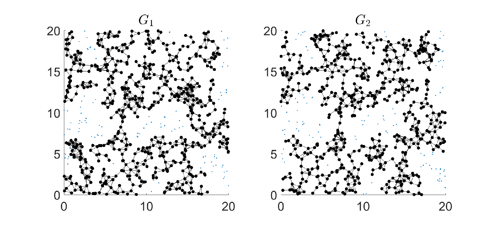
To verify the confidence intervals, we simulate within a square, for . Nodes in the largest mutual component are colored black, while the remaining nodes are colored blue. In Fig. 9, the node densities are at the upper confidence bound (), and there exists a mutual component that consists of a large fraction of nodes. In Fig. 10, the node densities are at the lower confidence bound (), and the size of the largest mutual component is small.

We next study the impact of interdependent distance on the percolation thresholds. Given , a smaller leads to a higher , since the probability that a node in has at least one supply nodes from decreases for a smaller . The effect is more significant when the number of nodes in is small. This is consistent with Fig. 11, where the increase of is more significant as decreases when is small.
The confidence intervals confirm that the reduced node density due to a lack of supply nodes is not sufficient to characterize the percolation of one of the interdependent graphs. The average density of nodes in that have at least one node within in is , given that is the probability that there is no node in within a disk area . If , with confidence, when , and when . We observe that the ranges of are different: when , and when . Intuitively, nodes in that have at least one supply nodes are clustered around the nodes in , smaller leads to a more clustered point process. The critical node density of a clustered point process is not the same as the critical node density of the homogeneous Poisson point process for percolation. More detailed study on the percolation of a clustered point process can be found in [21].

V Robustness of interdependent RGGs under random and geographical failures
Removing nodes independently at random with the same probability in one graph is equivalent to reducing the node density of the Poisson point process. To study the robustness of under random failures, the first step is to obtain the upper and lower bounds on percolation thresholds. With the bounds, we can determine which graph is able to resist more random node removals, by comparing the gap between the node density and the percolation threshold given (). The graph that can resist a smaller fraction of node removals is the bottleneck for the robustness of . Moreover, we are able to compute the maximum fraction of nodes that can be randomly removed from two graphs while guaranteeing to be percolated.
We next show that still percolates after a geographical attack that removes nodes in a finite connected region, if the node densities of the two graphs before the attack are above any upper bound on the percolation thresholds obtained in this paper (either analytical or simulation-based). Recall that we obtained upper bounds on the percolation thresholds of by mapping the percolation of to either the independent bond percolation on a square lattice or the 1-dependent bond percolation on a square lattice . Under both mappings, the event that a bond is open is entirely determined by the point processes in a finite region that contains the bond. After removing nodes of in a connected finite geographical region, the state of a bond may change from open to closed only if intersects the attack region. Let be the union of that intersects the attack region. The region is also a connected finite region. As long as or still percolates after setting bonds in to be closed, percolates.
Results from the percolation theory indeed indicate that setting all the bonds in a finite region to be closed does not affect the percolation of or . For any percolated , the probability that there exists a horizontal crossing of open bonds over a rectangle approaches 1 for any integer , as (Lemma 8 on Page 64 of [18]). The percolation of (after setting all bonds in to be closed) is justified by the fact that the connected open bonds across rectangles form a square annulus that does not intersect (shown in Fig. 12), which is a standard approach to prove the percolation of [18]. Moreover, the percolation of after all bonds in are set closed can be proved in the same approach, by noting that the probability that open bonds of form a horizontal crossing over a rectangle approaches 1 as the rectangle size increases to infinity [16].
If the rectangle is large but finite, the probability that a horizontal crossing formed by open bonds exists is close to 1 if or percolates. Therefore, the same analysis demonstrates the robustness of two finite interdependent RGGs under a geographical attack that removes the nodes in a disk region of size , where .

The robustness of interdependent RGGs under geographical failures is illustrated in Fig. 13. Nodes and links in the giant mutual component are colored black. The interdependent RGGs still percolate after all the nodes in a disk region are removed. This is in contrast with the cascading failures observed in [5] in the interdependent lattice model after an initial disk attack. One reason may be that every node can have more than one supply node in our model, while every node has only one supply node in [5]. The multiple localized interdependence helps the interdependent RGGs to resist geographical attacks.

VI Extensions to more general interdependence
In the previous sections, we studied a model where every node in is content to have at least one supply node in in the same mutual component (). The techniques can be extended to study models where every node in must have at least supply nodes from to receive enough supply, where can be either a constant or a random variable (). We briefly discuss the extensions to models with more general supply requirement using the example in Section III-A, where .
VI-A Deterministic supply requirement
The extension is straightforward if is a constant, . By the same discretization technique, the state of a site in the triangle lattice is determined by the point processes in a cell of area (recall Fig. 2). Declare a site to be open if there are at least nodes from in the cell that contains the site (). For each open site, every node from in the cell has at least supply nodes from in the same cell, satisfying the supply requirement. Following the same analysis as that in Section III-A, the percolation of the triangle lattice implies the percolation of .
For a Poisson point process of density , the probability that there are at least nodes in a cell of area is . An upper bound on the percolation thresholds is given by that satisfies:
VI-B Random supply requirement
Some extra work is necessary if is a random variable, . For simplicity, we first consider the case where is a constant and is a discrete random variable with a cumulative distribution function , . Furthermore, we assume that the number of supply nodes needed by every node in is independent. After the discretization, a site in the triangle lattice is open if the following two conditions are satisfied for at least one integer-valued .
- 1.
There are exactly nodes from in the cell.
- 2.
There are at least nodes from in the cell, each of which needs no more than supply nodes.
If both conditions are satisfied, at least nodes from and the nodes from each have enough supply. It is easy to see that the percolation of the triangle lattice still implies the percolation of .
Next we compute the probability that the two conditions are satisfied. The probability that there are nodes from in the cell is:
The probability that there are nodes from in the cell is:
The probability that a node in needs no more than supply nodes is . Since the number of supply nodes needed by every node in is independent, the probability that at least out of the nodes in each need no more than supply nodes is:
for , and for . By the law of total probability, for a given , the probability that there exist at least nodes from in the cell that each need no more than supply nodes is:
Since the events that there are exactly nodes from in the cell are mutually exclusive for distinct values of , using the law of total probability again, the probability that both conditions are satisfied is:
Any that satisfies is an upper bound on the percolation threshold of .
Finally, we consider the case where both and are discrete random variables. Suppose that nodes from are in the cell of area . If there exist integers , such that at least nodes from each need no more than supply nodes, then the nodes from all have enough supply (). However, it is difficult to obtain a clean formula of the probability that exists (to satisfy the condition). The events that exists are not mutually exclusive for distinct values of and . While it is possible to compute this probability using the inclusion-exclusion formula, the computation is expensive, since the number of choices of can be large and each term in the inclusion-exclusion formula requires the computation of order statistics.
A practical approach to estimate the probability that nodes have enough supply is by simulation. In each trial of the simulation, nodes are randomly generated in area , where follows a Poisson distribution of rate (). Then, each of the nodes is tagged with a realization of the random variable , which indicates the number of required supply nodes (). Let indicate whether there exist such that at least nodes among the nodes all have tags no more than (). The value of can be computed by Algorithm 3.
Initialization:
Sort the realizations of the random variable in the ascending order. Let be the sorted list (). Let .
Main loop:
We now prove the correctness of Algorithm 3. For easy presentation, the nodes are referred to as nodes in (). Initially, among the nodes in , the algorithm chooses one node that needs the smallest number of supply nodes. To support this node, at least nodes need to be in . If and , one node from and one node from suffice to support each other. Otherwise, if , at least nodes need to be in . The nodes must be supported by nodes from . If is larger than the total number of nodes in , then there are not enough supporting nodes in and . If and , then nodes from support nodes from , and vise versa. Note that and never decrease in the iterations, and at least one of them strictly increases in an iteration where is not determined. If there exists at least one pair , the algorithm terminates with at the smallest pair for both coordinates, which can be easily shown by contradiction. If no such pair exists, the algorithm terminates with .
Given , by repeating a sufficiently large number of trials, the probability that can be estimated within a small multiplicative error with high confidence using Monte Carlo simulation. As long as this probability is at least , percolates with high confidence.
VII Conclusion
We developed an interdependent RGG model for interdependent spatially embedded networks. We obtained analytical upper bounds and confidence intervals for the percolation thresholds. The percolation thresholds of two interdependent RGGs form a curve, which shows the tradeoff between the two node densities in order for the interdependent RGGs to percolate. The curve can be used to study the robustness of interdependent RGGs to random failures. Moreover, if the node densities are above any upper bound on the percolation thresholds obtained in this paper, then the interdependent RGGs remain percolated after a geographical attack. Finally, we extended the techniques to models with more general interdependence. The study of percolation thresholds in this paper can be used to design robust interdependent networks.
References
- [1] V. Rosato, L. Issacharoff, F. Tiriticco, S. Meloni, S. Porcellinis, and R. Setola, “Modelling interdependent infrastructures using interacting dynamical models,” International Journal of Critical Infrastructures, vol. 4, no. 1-2, pp. 63–79, 2008.
- [2] M. Parandehgheibi, K. Turitsyn, and E. Modiano, “Modeling the impact of communication loss on the power grid under emergency control,” in IEEE SmartGridComm, 2015.
- [3] S. V. Buldyrev, R. Parshani, G. Paul, H. E. Stanley, and S. Havlin, “Catastrophic cascade of failures in interdependent networks,” Nature, vol. 464, no. 7291, pp. 1025–1028, 2010.
- [4] A. Bashan, Y. Berezin, S. V. Buldyrev, and S. Havlin, “The extreme vulnerability of interdependent spatially embedded networks,” Nature Physics, vol. 9, no. 10, pp. 667–672, 2013.
- [5] Y. Berezin, A. Bashan, M. M. Danziger, D. Li, and S. Havlin, “Localized attacks on spatially embedded networks with dependencies,” Scientific reports, vol. 5, 2015.
- [6] J. Shao, S. V. Buldyrev, S. Havlin, and H. E. Stanley, “Cascade of failures in coupled network systems with multiple support-dependence relations,” Phys. Rev. E, vol. 83, p. 036116, Mar 2011.
- [7] O. Yağan, D. Qian, J. Zhang, and D. Cochran, “Optimal allocation of interconnecting links in cyber-physical systems: Interdependence, cascading failures, and robustness,” IEEE Transactions on Parallel and Distributed Systems, vol. 23, no. 9, pp. 1708–1720, 2012.
- [8] M. Franceschetti and R. Meester, Random networks for communication: from statistical physics to information systems. Cambridge University Press, 2008, vol. 24.
- [9] M. Franceschetti, O. Dousse, D. Tse, and P. Thiran, “Closing the gap in the capacity of wireless networks via percolation theory,” IEEE Trans. Inform. Theory, vol. 53, no. 3, pp. 1009–1018, March 2007.
- [10] Z. Kong and E. M. Yeh, “Resilience to degree-dependent and cascading node failures in random geometric networks,” IEEE Trans. Inform. Theory, vol. 56, no. 11, pp. 5533–5546, 2010.
- [11] M. Penrose, Random geometric graphs. Oxford Univ. Press, 2003.
- [12] R. Meester and R. Roy, Continuum percolation. Cambridge Univ. Press, 1996.
- [13] P. Balister, A. Sarkar, and B. Bollobás, “Percolation, connectivity, coverage and colouring of random geometric graphs,” in Handbook of Large-Scale Random Networks. Springer, 2008, pp. 117–142.
- [14] W. Li, A. Bashan, S. V. Buldyrev, H. E. Stanley, and S. Havlin, “Cascading failures in interdependent lattice networks: The critical role of the length of dependency links,” Physical review letters, vol. 108, no. 22, p. 228702, 2012.
- [15] P. Hall, “On continuum percolation,” The Annals of Probability, pp. 1250–1266, 1985.
- [16] P. Balister, B. Bollobás, and M. Walters, “Continuum percolation with steps in the square or the disc,” Random Structures and Algorithms, vol. 26, no. 4, pp. 392–403, 2005.
- [17] G. R. Grimmett, Percolation. Springer-Verlag Berlin Heidelberg, 1999.
- [18] B. Bollobás and O. Riordan, Percolation. Cambridge Univ. Press, 2006.
- [19] R. Roy, “The Russo-Seymour-Welsh theorem and the equality of critical densities and the “dual” critical densities for continuum percolation on ,” The Annals of Probability, pp. 1563–1575, 1990.
- [20] G. Casella and R. L. Berger, Statistical inference. Duxbury Pacific Grove, CA, 2002, vol. 2.
- [21] B. Błaszczyszyn and D. Yogeshwaran, “On comparison of clustering properties of point processes,” Advances in Applied Probability, vol. 46, no. 1, pp. 1–20, 2014.
![[Uncaptioned image]](1709.03032v2/jianan.png) |
Jianan Zhang received his B.E. degree in Electronic Engineering from Tsinghua University, Beijing, China, in 2012, and M.S. degree from Massachusetts Institute of Technology, Cambridge, MA, USA, in 2014. He is currently pursuing the Ph.D. degree at the Laboratory for Information and Decision Systems, Massachusetts Institute of Technology. His research interests include network robustness, optimization and interdependent networks. |
![[Uncaptioned image]](1709.03032v2/eyeh.png) |
Edmund M. Yeh (SM’12) received his B.S. in Electrical Engineering with Distinction and Phi Beta Kappa from Stanford University in 1994. He then studied at Cambridge University on the Winston Churchill Scholarship, obtaining his M.Phil in Engineering in 1995. He received his Ph.D. in Electrical Engineering and Computer Science from MIT in 2001. He is currently Professor of Electrical and Computer Engineering at Northeastern University. He was previously Assistant and Associate Professor of Electrical Engineering, Computer Science, and Statistics at Yale University. Professor Yeh has held visiting positions at MIT, Stanford, Princeton, University of California at Berkeley, New York University, Swiss Federal Institute of Technology Lausanne (EPFL), and Technical University of Munich. He has been on the technical staff at the Mathematical Sciences Research Center, Bell Laboratories, Lucent Technologies, Signal Processing Research Department, ATT Bell Laboratories, and Space and Communications Group, Hughes Electronics Corporation. Professor Yeh is the recipient of the Alexander von Humboldt Research Fellowship, the Army Research Office Young Investigator Award, the Winston Churchill Scholarship, the National Science Foundation and Office of Naval Research Graduate Fellowships, the Barry M. Goldwater Scholarship, the Frederick Emmons Terman Engineering Scholastic Award, and the President’s Award for Academic Excellence (Stanford University). He received Best Paper Awards at the ACM Conference on Information Centric Networking, Berlin, September 2017, at the IEEE International Conference on Communications (ICC), London, June 2015, and at the IEEE International Conference on Ubiquitous and Future Networks (ICUFN), Phuket, July 2012. |
![[Uncaptioned image]](1709.03032v2/eytan.png) |
Eytan Modiano received his B.S. degree in Electrical Engineering and Computer Science from the University of Connecticut at Storrs in 1986 and his M.S. and PhD degrees, both in Electrical Engineering, from the University of Maryland, College Park, MD, in 1989 and 1992 respectively. He was a Naval Research Laboratory Fellow between 1987 and 1992 and a National Research Council Post Doctoral Fellow during 1992-1993. Between 1993 and 1999 he was with MIT Lincoln Laboratory. Since 1999 he has been on the faculty at MIT, where he is a Professor and Associate Department Head in the Department of Aeronautics and Astronautics, and Associate Director of the Laboratory for Information and Decision Systems (LIDS). His research is on communication networks and protocols with emphasis on satellite, wireless, and optical networks. He is the co-recipient of the MobiHoc 2016 best paper award, the Wiopt 2013 best paper award, and the Sigmetrics 2006 Best paper award. He is the Editor-in-Chief for IEEE/ACM Transactions on Networking, and served as Associate Editor for IEEE Transactions on Information Theory and IEEE/ACM Transactions on Networking. He was the Technical Program co-chair for IEEE Wiopt 2006, IEEE Infocom 2007, ACM MobiHoc 2007, and DRCN 2015. He is a Fellow of the IEEE and an Associate Fellow of the AIAA, and served on the IEEE Fellows committee. |