跳到论文正文
W Papers独立论文阅读器 arXiv:1709.02604 论文正文 计算阅读时间 · 0%
引用这篇论文根据当前论文元数据生成,正式投稿前建议核对。


License: arXiv.org perpetual non-exclusive license
arXiv:1709.02604v1 [math.OC] 08 Sep 2017

Consensus under Misaligned Orientations

Hyo-Sung Ahn    Minh Hoang Trinh & Byung-Hun Lee ††thanks: $ˆ†$School of Mechanical Engineering, Gwangju Institute of Science and Technology (GIST), 123 Cheomdan-gwagiro, Buk-gu, Gwangju, Republic of Korea. E-mails: hyosung@gist.ac.kr,trinhhoangminh@gist.ac.kr, bhlee@gist.ac.kr
Abstract

This paper presents a consensus algorithm under misaligned orientations, which is defined as (i) misalignment to global coordinate frame of local coordinate frames, (ii) biases in control direction or sensing direction, or (iii) misaligned virtual global coordinate frames. After providing a mathematical formulation, we provide some sufficient conditions for consensus or for divergence. Besides the stability analysis, we also conduct some analysis for convergence characteristics in terms of locations of eigenvalues. Through a number of numerical simulations, we would attempt to understand the behaviors of misaligned consensus dynamics.

I Introduction

Consensus for multi-agent systems has been so widely studied for the last two decades [1, 2]. The consensus algorithms have been shown to be useful for various engineering applications such as mobile dispatch [3], energy coordination in smart building [4], smart grid [5], and so on. There also have been so various research efforts in terms of theoretical developments. According to dynamic models, there are a number of different analyses for continuous time, discrete-time, cluster consensus, homogeneous, heterogeneous systems, stochastic, lower-order, high-order systems, etc. Meanwhile, according to the network topologies, directed, undirected, switching, and balanced graphs have been studied. Depending upon characteristics of sampling, synchronous, asynchronous, event-triggered, and quantized-based consensus algorithms also have been investigated.

Given a network system, that is described by a graph 𝒢=(𝒱,ℰ)\mathcal{G}=(\mathcal{V},\mathcal{E}) where 𝒱={1,…,n}\mathcal{V}=\{1,\ldots,n\} is the set of agents and ℰ\mathcal{E} is the set of connectivities, however, the majority of existing consensus algorithms uses state information directly for control update. That is, when agent is modeled as p˙i=ui​(pi,pj),j∈𝒩i\dot{p}_{i}=u_{i}(p_{i},p_{j}),~j\in\mathcal{N}_{i}, where 𝒩i\mathcal{N}_{i} is the set of neighboring agents of agent ii, for the control update ui​(pi,pj)u_{i}(p_{i},p_{j}), the agent ii uses the state information pip_{i} and pjp_{j}. Since the agent ii uses only its own state information pip_{i} along with neighboring information pjp_{j}, the consensus update ui​(pi,pj)u_{i}(p_{i},p_{j}) may be considered as decentralized. However, observing that the states p1,p2,…,pnp_{1},p_{2},\ldots,p_{n} are all defined in a common global coordinate frame, we can notice that the control updates u1,u2,…,unu_{1},u_{2},\ldots,u_{n} are all defined in a common global coordinate frame. Thus, in this sense, most of existing consensus algorithms have been developed under the assumption of available global state information pip_{i} and pjp_{j}, or diffusively-coupling state information pi−pjp_{i}-p_{j}. Note that the diffusive coupling state information pi−pjp_{i}-p_{j}, where (i,j)∈ℰ(i,j)\in\mathcal{E}, are defined in a common direction in general setups although it can be transformed into local frames (see (2) in Section II).

In this paper, we would like to study a consensus problem under the setup of misaligned information of pi−pjp_{i}-p_{j} that has been rarely examined in existing works. That is, in this paper, it is supposed that the common directions representing pi−pjp_{i}-p_{j} may be different according to the sensing or control capability of agents. We are mainly motivated to consider certain situations where agents’ coordinate frames are misaligned, or sensing or control directions have been biased. In typical consensus algorithm given in (1), the summed diffusive coupling information −∑j∈𝒩iai​j(pi−pj)-\sum_{j\in\mathcal{N}_{i}}a_{ij}(p_{i}-p_{j}) are represented in a common direction, in ideal situations. However, it may be possible to imagine a circumstance where −∑j∈𝒩iai​j(pi−pj)-\sum_{j\in\mathcal{N}_{i}}a_{ij}(p_{i}-p_{j}) may be implemented in a wrong direction or biased direction, or the measurement pi−pjp_{i}-p_{j} may be biased. This paper seeks to find a consensus condition and attempts to understand the convergence characteristics under this circumstance. From literature search, it is observed that the consensus problem aforementioned has not been investigated directly; but some similar works have been studied. For examples, in [6, 7], the author studied a Cartesian coordinate coupling problem with a common coupling matrix CC, and in [8], they also studied a consensus problem with coupling multiplied by rotation matrix in 33-D for cyclic formations. However, in [6, 8], they did not consider a general case when agents have different misaligned orientation angles. In distributed formation control, the orientation alignment problem has been key issues [9, 10]. It was shown that when orientations of agents are aligned, the desired formation could be achieved. Related with the orientation misalignment, a consensus with pursuit weight [11], i.e., ki​j​ej​αi​jk_{ij}e^{j\alpha_{ij}}, may have some relevance. But, the pursuit system studied in [11] updates the control law after collecting the pursuit angles at each agent. In a different setup, which can be considered as orientation misalignment, rotation matrices were combined into the coupling terms in [12]. However, the ideas used in [11, 12] do not consider the misalignment of control actions. Thus, since the misalignment angle is defined as the same one for each agent in our problem, the problems studied in [11, 12] are different from our current work.

Consequently, the main contributions of this paper can be summarized as follows. First, we formulate a consensus problem with misaligned orientation angles in which agents may implement control actions into misaligned directions, or update the consensus algorithms with misaligned measurements. We provide some conditions for consensus. Second, we also further conduct an analysis to estimate the locations of eigenvalues that are closely related with the convergence characteristics. Then, based on analyses, we conduct numerical simulations to understand the behaviors of agents in a better way. As far as the authors are concerned, even though there have been some related works, there has been no direct research for consensus under misaligned orientations.

This paper consists of as follows. In Section II, we would like to formulate the consensus problem under misaligned orientations in a clear way. Then, in Section III, we provide analyses for consensus conditions and some related convergence characteristics. We present numerical illustrations in Section IV to validate the analyses and provide further discussions in Section V. Conclusions will be presented in Section VI.

II Problem Formulation

Let the global coordinate frame be denoted as Σg{}^{g}\Sigma and the ii-th local coordinate frame as Σi{}^{i}\Sigma. The position of agent ii is represented as pi∈ℝ2p_{i}\in\mathbb{R}^{2} in the global coordinate frame Σg{}^{g}\Sigma, where i∈{1,…,n}i\in\{1,\ldots,n\}. Given two position vectors pip_{i} and pjp_{j}, the displacement vector between pip_{i} and pjp_{j} is denoted as zi​j=pi−pjz_{ij}=p_{i}-p_{j}. The consensus algorithm for continuous-time linear systems is given as:

p˙i\displaystyle\dot{p}_{i} =−∑j∈𝒩iai​j(pi−pj)=−∑j∈𝒩iai​jzi​j\displaystyle=-\sum_{j\in\mathcal{N}_{i}}a_{ij}(p_{i}-p_{j})=-\sum_{j\in\mathcal{N}_{i}}a_{ij}z_{ij} (1)

where ai​j=aj​i∈{0,1}a_{ij}=a_{ji}\in\{0,1\} depending upon the connectivity of undirected graphs. The consensus problem (1) can be rewritten as

p˙ii\displaystyle{{}^{i}\dot{p}}_{i} =−∑j∈𝒩iai​j(pii−pji)=∑j∈𝒩iai​jpji\displaystyle=-\sum_{j\in\mathcal{N}_{i}}a_{ij}({{}^{i}p}_{i}-{{}^{i}p}_{j})=\sum_{j\in\mathcal{N}_{i}}a_{ij}{{}^{i}p}_{j} (2)

which controls the movement of agent in its own local coordinate frame Σi{}^{i}\Sigma. Obviously, the convergence property and stability of (1) and (2) are equivalent. However, the vector zi​jz_{ij} is expressed in the global coordinate frame Σg{}^{g}\Sigma, while the vector pji{{}^{i}p}_{j} is expressed in the local coordinate frame Σi{}^{i}\Sigma. Hence, the update of consensus algorithm could be done in two different scenarios. The first scenario, described in (1), is to use the vector zi​jz_{ij} in orientation aligned coordinate frame, which is the local coordinate frame aligned to the global frame. In Fig. 1, the orientation aligned coordinate frames are denoted as Σgi{{}^{g^{i}}\Sigma} (i.e., in this figure, they are Σg1{}^{g^{1}}\Sigma, Σg2{}^{g^{2}}\Sigma, and Σg3{}^{g^{3}}\Sigma in red color). Thus, in the first approach, the orientation needs to be aligned. The second scenario, described in (2), is to use pji{{}^{i}p}_{j} in the local coordinate frame Σi{}^{i}\Sigma, whose orientation is not aligned to the global frame. In Fig. 1, the local coordinate frames are denoted as Σ1{}^{1}\Sigma, Σ2{}^{2}\Sigma, and Σ3{}^{3}\Sigma in blue color. The first scenario (1) requires a constraint of alignment, while the second scenario (2) is free from this constraint. Thus, the second scenario is considered to be of more distributed in the sense that the vector pji{{}^{i}p}_{j} can be defined in local coordinate frames directly. It may be worthy of considering another scenario as follows: the local coordinate frames are not aligned; but agents have measured the positions pip_{i} in global coordinate frame (ex. using GPS information). In such case, they have to use zi​jz_{ij} in the global coordinate frame; but since the orientations are not aligned to Σg{}^{g}\Sigma, they need to sense the orientation angles or they need to find the direction of Σg{}^{g}\Sigma to calculate the orientation angles. In Fig. 1, the orientations are denoted as ϕi\phi_{i}. Then, using the obtained orientation angles ϕi\phi_{i}, agents can virtually rotate its local coordinate frame to global coordinate frame. Under this scenario, the coordinate frames Σgi{{}^{g^{i}}\Sigma} in Fig. 1 can be considered virtually aligned global coordinate frame.11 1 Note that with available orientation angles ϕi\phi_{i}, the vectors zi​jz_{ij} and pji{{}^{i}p}_{j} are related by pii−pji=D⁡(−ϕi)​(pi−pj)=D⁡(−ϕi)​zi​j=−pji\displaystyle{{}^{i}p}_{i}-{{}^{i}p}_{j}=D(-\phi_{i})(p_{i}-p_{j})=D(-\phi_{i})z_{ij}=-{{}^{i}p}_{j} (3) where D⁡(−ϕi)D(-\phi_{i}) is the rotation matrix. Thus, in terms of analysis, the three scenarios are equivalent. Then, the agent can implement the measurement pi−pj=zi​jp_{i}-p_{j}=z_{ij} into the virtual coordinate frame Σgi{{}^{g^{i}}\Sigma} for updating the consensus algorithm in global coordinate frame. This scenario may be considered the third scenario. Once again, note that the three scenarios have the same convergence and stability properties. In literature, there have been no distinctions between these three scenarios; however, in terms of sensing or in terms of implementation, they are essentially different and should be distinguished.

Refer to caption
Fig. 1: Global coordinate frame Σg{}^{g}\Sigma, local coordinate frames Σi{}^{i}\Sigma, virtually aligned global coordinate frames Σgi{{}^{g^{i}}\Sigma}, and orientation angles ϕi\phi_{i}.

As the main motivation of this paper, let us suppose that there are some errors in the orientation alignment, or orientation estimation in these three scenarios. Under the first scenario, the orientations of aligned local coordinate frames Σgi{}^{g^{i}}\Sigma, which are supposed to be aligned to the global frame Σg{}^{g}\Sigma, may be not aligned as illustrated in Fig. 2(a). That is, the local coordinate frame Σgi{}^{g^{i}}\Sigma, which is supposed to be aligned to Σg{}^{g}\Sigma, has in fact misalignment error as much as θi\theta_{i}. Under the second scenario, the agent ii may measure the direction of neighboring agent jj with angle error θi\theta_{i}. In Fig. 2(b), the agent 11 measures the agent 22 with direction error θ1\theta_{1}. This can be interpreted as an error in control direction. Even though the displacement measurement is correct, during the implementation process, the agent may provide control command to wrong direction with orientation bias θi\theta_{i}. Under the third scenario, it can be assumed that the virtually aligned global coordinate frames have misalignment errors as θi\theta_{i} as also illustrated in Fig. 2(c). Then, the third scenario would have the same alignment problem as the first scenario.

Refer to caption
(a) Misalignment orientation errors in scenario 11.
Refer to caption
(b) Misaligned orientation biases in scenario 22.
Refer to caption
(c) Misalignment orientation errors in scenario 33.
Fig. 2: Misalignment errors in three scenarios.

Without notational confusion, the orientation errors or biases considered in the above three scenarios are called misaligned orientation errors. The misaligned orientation errors may be due to errors in alignment to the global coordinate frame, biases in local sensing or in control direction, or errors in virtual alignment. With the presence of the error θi\theta_{i}, during the implementation, it can be represented in wrong directions. For example, it may be represented in the misaligned virtual coordinate frames as depicted in Fig. 2(c). Thus, the control inputs transformed to the global coordinate frame Σg{}^{g}\Sigma would be defined as

p˙i\displaystyle\dot{p}_{i} =−D(θi)∑j∈𝒩iai​j(pi−pj)\displaystyle=-D(\theta_{i})\sum_{j\in\mathcal{N}_{i}}a_{ij}(p_{i}-p_{j})
=−∑j∈𝒩iai​jD(θi)(pi−pj)\displaystyle=-\sum_{j\in\mathcal{N}_{i}}a_{ij}D(\theta_{i})(p_{i}-p_{j}) (4)

Note that in the above equation, D⁡(θi)D(\theta_{i}) is a S​O​(2)SO(2) rotation matrix and the graph can be considered as directed, although the neighboring agents ii and jj mutually sense each other and exchange the information, since the weights for edges have the relationship ai​j​D​(θi)≠aj​i​D​(θj)a_{ij}D(\theta_{i})\neq a_{ji}D(\theta_{j}) even though ai​j=aj​ia_{ij}=a_{ji}. Then if we consider ai​j​D​(θi)a_{ij}D(\theta_{i}) as edge weighing, it is a matrix-weighted directed graph [13, 14]. Let us define adjacency edge-matrix as Ai​j=ai​j​D​(θi)A_{ij}=a_{ij}D(\theta_{i}). Then, the adjacency matrix is given as

𝒜\displaystyle\mathcal{A} =[Ai​j]\displaystyle=[A_{ij}]
=[0a12​D​(θ1)a13​D​(θ1)⋯a1​n​D​(θ1)a21​D​(θ2)0a23​D​(θ2)⋯a2​n​D​(θ2)⋮⋮an​1​D​(θn)⋯0]∈ℝ2​n×2​n\displaystyle=\left[\begin{array}[]{ccccc}0&a_{12}D(\theta_{1})&a_{13}D(\theta_{1})&\cdots&a_{1n}D(\theta_{1})\\ a_{21}D(\theta_{2})&0&a_{23}D(\theta_{2})&\cdots&a_{2n}D(\theta_{2})\\ \vdots&&&&\vdots\\ a_{n1}D(\theta_{n})&\cdots&&&0\end{array}\right]\in\mathbb{R}^{2n\times 2n}

For agent ii, we define out-degree matrix as Dio​u​t=∑j∈𝒩iai​j​D​(θi)D_{i}^{out}=\sum_{j\in\mathcal{N}_{i}}a_{ij}D(\theta_{i}) and in-degree matrix as Dii​n=∑j∈𝒩iaj​i​D​(θj)D_{i}^{in}=\sum_{j\in\mathcal{N}_{i}}a_{ji}D(\theta_{j}). Sincerely it is clear that Dio​u​t≠Dii​n{D}_{i}^{out}\neq{D}_{i}^{in}, it is not balanced. Then, we can define a block out-degree matrix of 𝒢\mathcal{G} as 𝒟o​u​t=blkdiag​[Dio​u​t]\mathcal{D}^{out}=\text{blkdiag}[D_{i}^{out}]. Then, the SO(2)-weighted Laplacian matrix can be generated as

ℒo​u​t=𝒟o​u​t−𝒜\displaystyle\mathcal{L}^{out}=\mathcal{D}^{out}-\mathcal{A} (9)

Using the above Laplacian matrix, we can have the state propagation as

p˙=−ℒo​u​t​p​(t)\displaystyle\dot{p}=-\mathcal{L}^{out}p(t) (10)

where p=(p1T,p2T,…,pnT)T∈ℝ2​np=(p_{1}^{T},p_{2}^{T},\ldots,p_{n}^{T})^{T}\in\mathbb{R}^{2n}.

III Convergence and stability analysis

This section is dedicated to the convergence and stability analysis of the system (10). The following lemmas are developed for convergence analysis.

Lemma 1

The Laplacian matrix ℒo​u​t\mathcal{L}^{out} has rank as rank​(ℒo​u​t)=2​n−2\text{rank}(\mathcal{L}^{out})=2n-2, and the null space is given as 𝒩⁡(ℒo​u​t)=span​{[1,0,1,0,⋯,1,0]⏟≜1e∈ℝ2​nT,[0,1,0,1,⋯,0,1]⏟≜1o∈ℝ2​nT}\mathcal{N}(\mathcal{L}^{out})=\text{span}\{{\underbrace{[1,0,1,0,\cdots,1,0]}_{\triangleq{\bf}{1}^{e}\in\mathbb{R}^{2n}}}^{T},{\underbrace{[0,1,0,1,\cdots,0,1]}_{\triangleq{\bf}{1}^{o}\in\mathbb{R}^{2n}}}^{T}\}.

Proof:

Defining q=c1​1e+c2​1o≜qe+qoq=c_{1}{\bf}{1}^{e}+c_{2}{\bf}{1}^{o}\triangleq q^{e}+q_{o}, where c1c_{1} and c2c_{2} are constants, we have ℒo​u​t​q=0\mathcal{L}^{out}q=0. Let us examine the converse. From (4), equalizing p˙i=0\dot{p}_{i}=0, we will show that ∑j∈𝒩iai​j​D​(θi)​(pi−pj)=0\sum_{j\in\mathcal{N}_{i}}a_{ij}D(\theta_{i})(p_{i}-p_{j})=0 only when pi=pjp_{i}=p_{j}. Denoting pi=(xi,yi)Tp_{i}=(x_{i},y_{i})^{T}, we can write

∑j∈𝒩iai​j​D​(θi)​(pi−pj)\displaystyle\sum_{j\in\mathcal{N}_{i}}a_{ij}D(\theta_{i})(p_{i}-p_{j}) =[cos⁡θi−sin⁡θisin⁡θicos⁡θi]​∑j∈𝒩iai​j​[xi−xjyi−yj]\displaystyle=\left[\begin{array}[]{cc}\cos\theta_{i}&-\sin\theta_{i}\\ \sin\theta_{i}&\cos\theta_{i}\end{array}\right]\sum_{j\in\mathcal{N}_{i}}a_{ij}\left[\begin{array}[]{c}x_{i}-x_{j}\\ y_{i}-y_{j}\end{array}\right]
=[cos⁡θi−sin⁡θisin⁡θicos⁡θi]​[∑j∈𝒩iai​j​(xi−xj)∑j∈𝒩iai​j​(yi−yj)]\displaystyle=\left[\begin{array}[]{cc}\cos\theta_{i}&-\sin\theta_{i}\\ \sin\theta_{i}&\cos\theta_{i}\end{array}\right]\left[\begin{array}[]{c}\sum_{j\in\mathcal{N}_{i}}a_{ij}(x_{i}-x_{j})\\ \sum_{j\in\mathcal{N}_{i}}a_{ij}(y_{i}-y_{j})\end{array}\right]

Since the matrix D⁡(θi)D(\theta_{i}) is non-singular, in order to get p˙i=0\dot{p}_{i}=0, we only need to have ∑j∈𝒩iai​j​(xi−xj)=0\sum_{j\in\mathcal{N}_{i}}a_{ij}(x_{i}-x_{j})=0 and ∑j∈𝒩iai​j​(yi−yj)=0\sum_{j\in\mathcal{N}_{i}}a_{ij}(y_{i}-y_{j})=0, which is the consensus in xx-component and yy-component respectively. Consequently, it proves that rank​(ℒo​u​t)=2​n−2\text{rank}(\mathcal{L}^{out})=2n-2. ∎

Lemma 2

The set of eigenvalues of ℒo​u​t\mathcal{L}^{out} contains only two zero eigenvalues corresponding to eigenvectors span​{1e}\text{span}\{{\bf}{1}^{e}\} and span​{1o}\text{span}\{{\bf}{1}^{o}\} respectively.

Proof:

The Laplacian matrix is given as

ℒo​u​t\displaystyle\mathcal{L}^{out} =[∑j∈𝒩1a1​j​D​(θ1)−a12​D​(θ1)−a13​D​(θ1)⋯−a1​n​D​(θ1)−a21​D​(θ2)∑j∈𝒩2a2​j​D​(θ2)−a23​D​(θ2)⋯−a2​n​D​(θ2)⋮⋮−an​1​D​(θn)⋯∑j∈𝒩nan​j​D​(θn)]\displaystyle=\left[\begin{array}[]{ccccc}\sum_{j\in\mathcal{N}_{1}}a_{1j}D(\theta_{1})&-a_{12}D(\theta_{1})&-a_{13}D(\theta_{1})&\cdots&-a_{1n}D(\theta_{1})\\ -a_{21}D(\theta_{2})&\sum_{j\in\mathcal{N}_{2}}a_{2j}D(\theta_{2})&-a_{23}D(\theta_{2})&\cdots&-a_{2n}D(\theta_{2})\\ \vdots&&&&\vdots\\ -a_{n1}D(\theta_{n})&\cdots&&&\sum_{j\in\mathcal{N}_{n}}a_{nj}D(\theta_{n})\end{array}\right]

Defining mi=∑j=1nai​jm_{i}=\sum_{j=1}^{n}a_{ij}, we can see that for each row vector, it has its diagonal component as micosθim_{i}\cos\theta_{i} and off diagonal components as −misinθi-m_{i}\sin\theta_{i}, ai​jsinθi,a_{ij}\sin\theta_{i}, and −ai​jcosθi-a_{ij}\cos\theta_{i}, ∀j∈𝒩i\forall j\in\mathcal{N}_{i}, or misinθim_{i}\sin\theta_{i}, −ai​jsinθi,-a_{ij}\sin\theta_{i}, and ai​jcosθia_{ij}\cos\theta_{i}, ∀j∈𝒩i\forall j\in\mathcal{N}_{i}. Thus, the summation of elements of each row vector is zero, which completes the proof. ∎

It seems to be not trivial to show that all the eigenvalues of ℒo​u​t\mathcal{L}^{out} are on the right-half plane (RHP) except two zero eigenvalues when 0<cos⁡θi≤10<\cos\theta_{i}\leq 1. The following discussion and theorem are for this result. Let us decompose ℒo​u​t\mathcal{L}^{out} as

ℒo​u​t\displaystyle\mathcal{L}^{out} =[D⁡(θ1)00⋯00D⁡(θ2)0⋯0⋮⋱⋮0⋯D⁡(θn)]\displaystyle=\left[\begin{array}[]{ccccc}D(\theta_{1})&0&0&\cdots&0\\ 0&D(\theta_{2})&0&\cdots&0\\ \vdots&&\ddots&&\vdots\\ 0&\cdots&&&D(\theta_{n})\end{array}\right]
×[∑j∈𝒩1a1​j​I2−a12​I2−a13​I2⋯−a1​n​I2−a21​I2∑j∈𝒩2a2​j​I2−a23​I2⋯−a2​n​I2⋮⋱⋮−an​1​I2⋯∑j∈𝒩nan​j​I2]\displaystyle\times\left[\begin{array}[]{ccccc}\sum_{j\in\mathcal{N}_{1}}a_{1j}I_{2}&-a_{12}I_{2}&-a_{13}I_{2}&\cdots&-a_{1n}I_{2}\\ -a_{21}I_{2}&\sum_{j\in\mathcal{N}_{2}}a_{2j}I_{2}&-a_{23}I_{2}&\cdots&-a_{2n}I_{2}\\ \vdots&&\ddots&&\vdots\\ -a_{n1}I_{2}&\cdots&&&\sum_{j\in\mathcal{N}_{n}}a_{nj}I_{2}\end{array}\right]
≜blkdiag​[D⁡(θi)]⋅ℒo≜DD⁡(θi)⋅ℒo\displaystyle\triangleq\text{blkdiag}[D(\theta_{i})]\cdot\mathcal{L}^{o}\triangleq D_{D(\theta_{i})}\cdot\mathcal{L}^{o} (31)

where DD⁡(θi)D_{D(\theta_{i})} is a block diagonal matrix and ℒo=ℒoT\mathcal{L}^{o}={\mathcal{L}^{o}}^{T} is the Laplacian matrix characterizing the topology only (let us call it topology Laplacian matrix). With the above decomposition, the dynamics (10) is rewritten as

p˙=−(DD⁡(θi)​ℒo)​p​(t)\displaystyle\dot{p}=-(D_{D(\theta_{i})}\mathcal{L}^{o})p(t) (32)
Theorem 1

Let 0<cos⁡θi≤10<\cos\theta_{i}\leq 1. Then, the system described by (10) is globally asymptotically stable to a consensus value and eigenvalues of ℒo​u​t\mathcal{L}^{out} have positive-real parts except two zero eigenvalues.

Proof:

It is clear that the topology Laplacian matrix ℒo\mathcal{L}^{o} has two eigenvectors u1u_{1} and u2u_{2} correspoding to two zero eigenvalues. Let the topology Laplacian matrix ℒo\mathcal{L}^{o} be decomposed as UT​ℒo​U=diag​(λ1,λ2,…,λ2​n)U^{T}\mathcal{L}^{o}U=\text{diag}(\lambda_{1},\lambda_{2},\ldots,\lambda_{2n}) where λ1=λ2=0<λ3=λ4≤…​λ2​k−1=λ2​k​…≤λ2​n−1=λ2​n\lambda_{1}=\lambda_{2}=0<\lambda_{3}=\lambda_{4}\leq\ldots\lambda_{2k-1}=\lambda_{2k}\ldots\leq\lambda_{2n-1}=\lambda_{2n} and U=[u1,u2,u3,…,u2​n−1,u2​n]∈ℝ2​n×2​nU=[u_{1},u_{2},u_{3},\ldots,u_{2n-1},u_{2n}]\in\mathbb{R}^{2n\times 2n} is the orthogonal matrix composed of eigenvectors of ℒo\mathcal{L}^{o}. Thus, we have u1=c3​qeu_{1}=c_{3}q^{e} and u2=c4​qou_{2}=c_{4}q^{o} where c3c_{3} and c4c_{4} are constants, and U−1=UTU^{-1}=U^{T}. Let us define another matrix U′=[u3,…,u2​n−1,u2​n]∈ℝ2​n×(2​n−2)U^{\prime}=[u_{3},\ldots,u_{2n-1},u_{2n}]\in\mathbb{R}^{2n\times(2n-2)}. Then, we can have

UT​ℒo​U=[02×202×2​n−202​n−2×2(U′)T​ℒo​U′]\displaystyle U^{T}\mathcal{L}^{o}U=\left[\begin{array}[]{cc}0_{2\times 2}&0_{2\times{2n-2}}\\ 0_{{2n-2}\times 2}&(U^{\prime})^{T}\mathcal{L}^{o}U^{\prime}\\ \end{array}\right]

It is clear that (U′)T​ℒo​U′(U^{\prime})^{T}\mathcal{L}^{o}U^{\prime} is positive definite. Let p′=(U′)T​p∈ℝ2​n−2p^{\prime}=(U^{\prime})^{T}p\in\mathbb{R}^{2n-2}. Next, let us select a Lyapunov candidate as

V=(p′)T​(U′)T​ℒo​U′​p′\displaystyle V=(p^{\prime})^{T}(U^{\prime})^{T}\mathcal{L}^{o}U^{\prime}p^{\prime} (35)

The derivative is obtained as V˙=−(p˙′)T​(U′)T​ℒo​U′​p′−(p′)T​(U′)T​ℒo​U′​p˙′=−(p˙)T​U′​(U′)T​ℒo​U′​(U′)T​p\dot{V}=-(\dot{p}^{\prime})^{T}(U^{\prime})^{T}\mathcal{L}^{o}U^{\prime}p^{\prime}-({p}^{\prime})^{T}(U^{\prime})^{T}\mathcal{L}^{o}U^{\prime}\dot{p}^{\prime}=-(\dot{p})^{T}U^{\prime}(U^{\prime})^{T}\mathcal{L}^{o}U^{\prime}(U^{\prime})^{T}p −(p)T​U′​(U′)T​ℒo​U′​(U′)T​p˙-({p})^{T}U^{\prime}(U^{\prime})^{T}\mathcal{L}^{o}U^{\prime}(U^{\prime})^{T}\dot{p}. It can be shown that U′​(U′)T​ℒo​U′​(U′)T=ℒoU^{\prime}(U^{\prime})^{T}\mathcal{L}^{o}U^{\prime}(U^{\prime})^{T}=\mathcal{L}^{o}. Let [u1,u2]=z[u_{1},u_{2}]=z and [u1,u2]T=zT[u_{1},u_{2}]^{T}=z^{T}. Then, from U=[z,U′]U=[z,U^{\prime}], we have U​UT=z​zT+U′​U′T=I2​n×2​nUU^{T}=zz^{T}+U^{\prime}{U^{\prime}}^{T}=I_{2n\times 2n}, which means that U′​U′T=I2​n×2​n−z​zTU^{\prime}{U^{\prime}}^{T}=I_{2n\times 2n}-zz^{T}. Hence U′​(U′)T​ℒo​U′​(U′)T=(I2​n×2​n−z​zT)​ℒo​(I2​n×2​n−z​zT)=(I2​n×2​n−z​zT)​(ℒo−ℒo​z​zT)=(I2​n×2​n−z​zT)​ℒo=ℒo−z​zT​ℒo=ℒoU^{\prime}(U^{\prime})^{T}\mathcal{L}^{o}U^{\prime}(U^{\prime})^{T}=(I_{2n\times 2n}-zz^{T})\mathcal{L}^{o}(I_{2n\times 2n}-zz^{T})=(I_{2n\times 2n}-zz^{T})(\mathcal{L}^{o}-\mathcal{L}^{o}zz^{T})=(I_{2n\times 2n}-zz^{T})\mathcal{L}^{o}=\mathcal{L}^{o}-zz^{T}\mathcal{L}^{o}=\mathcal{L}^{o} due to ℒo​z=0\mathcal{L}^{o}z=0 and zT​ℒo=0z^{T}\mathcal{L}^{o}=0. Therefore, we obtain

V˙\displaystyle\dot{V} =−(p˙)T​ℒo​p−(p)T​ℒo​p˙\displaystyle=-(\dot{p})^{T}\mathcal{L}^{o}p-({p})^{T}\mathcal{L}^{o}\dot{p}
=−pT​ℒoT​DD⁡(θi)T​ℒo​p−(p)T​ℒo​DD⁡(θi)​ℒo​p\displaystyle=-p^{T}{\mathcal{L}^{o}}^{T}D_{D(\theta_{i})}^{T}\mathcal{L}^{o}p-({p})^{T}\mathcal{L}^{o}D_{D(\theta_{i})}\mathcal{L}^{o}p
=−(ℒo​p)T​[DD⁡(θi)T+DD⁡(θi)]​(ℒo​p)≤0\displaystyle=-(\mathcal{L}^{o}p)^{T}\left[D_{D(\theta_{i})}^{T}+D_{D(\theta_{i})}\right](\mathcal{L}^{o}p)\leq 0 (36)

The last inequality holds since DD⁡(θi)T+D⁡(θi)>0D_{D(\theta_{i})}^{T}+{D(\theta_{i})}>0 if 0<cos⁡θi≤10<\cos\theta_{i}\leq 1. It is now clear that (ℒo​p)T​(DD⁡(θi)T+DD⁡(θi))​(ℒo​p)=0(\mathcal{L}^{o}p)^{T}(D_{D(\theta_{i})}^{T}+D_{D(\theta_{i})})(\mathcal{L}^{o}p)=0 if and only if ℒo​p=0\mathcal{L}^{o}p=0, which implies that pp converges to a consensus and does not diverge because of p˙=0\dot{p}=0. ∎

The above Theorem 1 provides the condition for the consensus when 0<cos⁡θi≤10<\cos\theta_{i}\leq 1. Let some θi\theta_{i} be negative as θi<0\theta_{i}<0. Then some diagonal elements of DD⁡(θi)T+DD⁡(θi)D_{D(\theta_{i})}^{T}+D_{D(\theta_{i})} will be negative. However, even with some negative diagonal elements of DD⁡(θi)T+DD⁡(θi)D_{D(\theta_{i})}^{T}+D_{D(\theta_{i})}, V˙>0\dot{V}>0 is not ensured. Thus, even with some negative θi\theta_{i}, the instability is not ensured. Also, the Theorem 1 does not provide the locations of eigenvalues, which is related with the convergence characteristics. To evaluate the location of eigenvalues, we use Gershgorin circle for block matrix [15, 16], which is summarized as follows:

Lemma 3

Given a block matrix A=[Ai​j]A=[A_{ij}], all eigenvalues of AA are contained in the set G=∑i=1n∪GiG=\sum_{i=1}^{n}\cup G_{i} where GiG_{i} is the set of all λ∈ℂ\lambda\in\mathbb{C} satisfying

‖(Ai​i−λ​I2)−1‖−1≤∑j=1,j≠in‖Ai​j‖\displaystyle\|(A_{ii}-\lambda I_{2})^{-1}\|^{-1}\leq\sum_{j=1,j\neq i}^{n}\|A_{ij}\| (37)
Theorem 2

If agent ii is misaligned as cos⁡θi<1\cos\theta_{i}<1, then its eigenvalues are within the circles with center (micosθi,±misinθi)(m_{i}\cos\theta_{i},\pm m_{i}\sin\theta_{i}) and with radius mim_{i} in the complex domain, where mim_{i} is the cardinality of 𝒩i\mathcal{N}_{i}.

Proof:

From Lemma 3, we know that eigenvalues λi\lambda_{i} of each row block matrix satisfy the following inequality:

‖(∑j∈𝒩iai​j​D​(θi)−λi​I2)−1‖−1\displaystyle\left\|\left(\sum_{j\in\mathcal{N}_{i}}a_{ij}D(\theta_{i})-\lambda_{i}I_{2}\right)^{-1}\right\|^{-1} ≤∑j∈𝒩i,j≠in‖ai​j​D​(θi)‖\displaystyle\leq\sum_{j\in\mathcal{N}_{i},j\neq i}^{n}\|a_{ij}D(\theta_{i})\|
⟺‖(mi​D​(θi)−λi​I2)−1‖−1\displaystyle\Longleftrightarrow\left\|\left(m_{i}D(\theta_{i})-\lambda_{i}I_{2}\right)^{-1}\right\|^{-1} ≤mi​‖D⁡(θi)‖\displaystyle\leq m_{i}\|D(\theta_{i})\| (38)

Since singular value of a SO(2) matrix is 11, we can change the above inequality as

‖(D⁡(θi)−λimi​I2)−1‖−1\displaystyle\left\|\left(D(\theta_{i})-\frac{\lambda_{i}}{m_{i}}I_{2}\right)^{-1}\right\|^{-1} ≤1\displaystyle\leq 1
⟺‖(D⁡(θi)−λimi​I2)−1‖\displaystyle\Longleftrightarrow\left\|\left(D(\theta_{i})-\frac{\lambda_{i}}{m_{i}}I_{2}\right)^{-1}\right\| ≥1\displaystyle\geq 1 (39)

The inverse of the left-hand side can be obtained as:

(D⁡(θi)−λimi​I2)−1=11mi2​λi2−2cosθimi​λi+1​[cos⁡θi−λimisin⁡θi−sin⁡θicos⁡θi−λimi]⏟≜P\displaystyle\left(D(\theta_{i})-\frac{\lambda_{i}}{m_{i}}I_{2}\right)^{-1}=\underbrace{\frac{1}{\frac{1}{m_{i}^{2}}\lambda_{i}^{2}-\frac{2\cos\theta_{i}}{m_{i}}\lambda_{i}+1}\left[\begin{array}[]{cc}\cos\theta_{i}-\frac{\lambda_{i}}{m_{i}}&\sin\theta_{i}\\ -\sin\theta_{i}&\cos\theta_{i}-\frac{\lambda_{i}}{m_{i}}\end{array}\right]}_{\triangleq P}

Denote λimi≜κi=αi+j​βi\frac{\lambda_{i}}{m_{i}}\triangleq\kappa_{i}=\alpha_{i}+j\beta_{i} and λi∗mi≜κi∗=αi−j​βi\frac{\lambda_{i}^{\ast}}{m_{i}}\triangleq\kappa_{i}^{\ast}=\alpha_{i}-j\beta_{i}, where λi∗\lambda_{i}^{\ast} is the conjugate of λi\lambda_{i}. Then, in order to use the relationship ‖P‖=λm​a​x​(P∗​P)\|P\|=\sqrt{\lambda_{max}(P^{\ast}P)}, where P∗P^{\ast} is a complex conjugate of PP, P∗​PP^{\ast}P can be obtained as:

P∗​P\displaystyle P^{\ast}P =1(κ∗i2−2cosθiκi∗+1)(κi2−2cosθiκi+1)\displaystyle=\frac{1}{({\kappa^{\ast}}_{i}^{2}-2\cos\theta_{i}{\kappa}_{i}^{\ast}+1)({\kappa}_{i}^{2}-2\cos\theta_{i}{\kappa}_{i}+1)}
×[cos⁡θi−κi∗−sin⁡θisin⁡θicos⁡θi−κi∗]​[cos⁡θi−κisin⁡θi−sin⁡θicos⁡θi−κi]⏟≜𝐓\displaystyle\times\underbrace{\left[\begin{array}[]{cc}\cos\theta_{i}-\kappa_{i}^{\ast}&-\sin\theta_{i}\\ \sin\theta_{i}&\cos\theta_{i}-\kappa_{i}^{\ast}\end{array}\right]\left[\begin{array}[]{cc}\cos\theta_{i}-\kappa_{i}&\sin\theta_{i}\\ -\sin\theta_{i}&\cos\theta_{i}-\kappa_{i}\end{array}\right]}_{\triangleq\mathbf{T}}

It is noticeable that κi∗2−2cosθiκi∗+1{\kappa_{i}^{\ast}}^{2}-2\cos\theta_{i}\kappa_{i}^{\ast}+1 and κi2−2cosθiκi+1{\kappa}_{i}^{2}-2\cos\theta_{i}{\kappa}_{i}+1 can be decomposed as

κi∗2−2cosθiκi∗+1\displaystyle{\kappa_{i}^{\ast}}^{2}-2\cos\theta_{i}\kappa_{i}^{\ast}+1 =(κi∗−cosθi−jsinθi)(κi∗−cosθi+jsinθi)\displaystyle=(\kappa_{i}^{\ast}-\cos\theta_{i}-j\sin\theta_{i})({\kappa}_{i}^{\ast}-\cos\theta_{i}+j\sin\theta_{i})
κi2−2cosθiκi+1\displaystyle{\kappa}_{i}^{2}-2\cos\theta_{i}{\kappa}_{i}+1 =(κi−cosθi+jsinθi)(κi−cosθi−jsinθi)\displaystyle=({\kappa}_{i}-\cos\theta_{i}+j\sin\theta_{i})({\kappa}_{i}-\cos\theta_{i}-j\sin\theta_{i})

Then, (κi∗2−2cosθiκi∗+1)(κi2−2cosθiκi+1)({\kappa_{i}^{\ast}}^{2}-2\cos\theta_{i}\kappa_{i}^{\ast}+1)({\kappa}_{i}^{2}-2\cos\theta_{i}{\kappa}_{i}+1) can be rewritten as

(κi∗2−2cosθiκi∗+1)(κi2−2cosθiκi+1)\displaystyle({\kappa_{i}^{\ast}}^{2}-2\cos\theta_{i}{\kappa_{i}^{\ast}}+1)({\kappa}_{i}^{2}-2\cos\theta_{i}{\kappa}_{i}+1)
=(κi∗−cosθi−jsinθi)(κi∗−cosθi+jsinθi)\displaystyle~~~~~=({\kappa_{i}^{\ast}}-\cos\theta_{i}-j\sin\theta_{i})({\kappa_{i}^{\ast}}-\cos\theta_{i}+j\sin\theta_{i})
×(κi−cosθi+jsinθi)(κi−cosθi−jsinθi)\displaystyle~~~~~~~~~~\times({\kappa}_{i}-\cos\theta_{i}+j\sin\theta_{i})({\kappa}_{i}-\cos\theta_{i}-j\sin\theta_{i})
=(κi∗−cosθi−jsinθi)(κi−cosθi+jsinθi)\displaystyle~~~~~=({\kappa_{i}^{\ast}}-\cos\theta_{i}-j\sin\theta_{i})({\kappa}_{i}-\cos\theta_{i}+j\sin\theta_{i})
×(κi∗−cosθi+jsinθi)(κi−cosθi−jsinθi)\displaystyle~~~~~~~~~~\times({\kappa_{i}^{\ast}}-\cos\theta_{i}+j\sin\theta_{i})({\kappa}_{i}-\cos\theta_{i}-j\sin\theta_{i})
=(κi∗κi−κi∗cosθi+jκi∗sinθi−κicosθi−jκisinθi+1)⏟≜ξi∗\displaystyle~~~~~=\underbrace{({\kappa_{i}^{\ast}}\kappa_{i}-{\kappa_{i}^{\ast}}\cos\theta_{i}+j{\kappa_{i}^{\ast}}\sin\theta_{i}-\kappa_{i}\cos\theta_{i}-j\kappa_{i}\sin\theta_{i}+1)}_{\triangleq\xi_{i}^{\ast}}
×(κi∗κi−κi∗cosθi−jκi∗sinθi−κicosθi+jκisinθi+1)⏟≜ξi\displaystyle~~~~~~~~~~\times\underbrace{({\kappa_{i}^{\ast}}\kappa_{i}-{\kappa_{i}^{\ast}}\cos\theta_{i}-j{\kappa_{i}^{\ast}}\sin\theta_{i}-\kappa_{i}\cos\theta_{i}+j\kappa_{i}\sin\theta_{i}+1)}_{\triangleq\xi_{i}} (46)

Meanwhile the eigenvalues of 𝐓\mathbf{T} are obtained as 1−κicosθi−κi∗cosθi+κi∗κi±j(κisinθi−κi∗sinθi)1-\kappa_{i}\cos\theta_{i}-{\kappa_{i}^{\ast}}\cos\theta_{i}+{\kappa_{i}^{\ast}}\kappa_{i}\pm j(\kappa_{i}\sin\theta_{i}-{\kappa_{i}^{\ast}}\sin\theta_{i}), which are conjugate pair and equivalent to ξi\xi_{i} or ξi∗\xi_{i}^{\ast}. Furthermore, we can see that 1−κicosθi−κi∗cosθi+κi∗κi±j(κisinθi−κi∗sinθi)=1−2αicosθi+αi2+βi2±2βisinθi=(αi−cosθi)2+(βi±sinθi)2≥01-\kappa_{i}\cos\theta_{i}-{\kappa_{i}^{\ast}}\cos\theta_{i}+{\kappa_{i}^{\ast}}\kappa_{i}\pm j(\kappa_{i}\sin\theta_{i}-{\kappa_{i}^{\ast}}\sin\theta_{i})=1-2\alpha_{i}\cos\theta_{i}+\alpha_{i}^{2}+\beta_{i}^{2}\pm 2\beta_{i}\sin\theta_{i}=(\alpha_{i}-\cos\theta_{i})^{2}+(\beta_{i}\pm\sin\theta_{i})^{2}\geq 0. Thus, when λi=micosθi∓jmisinθi\lambda_{i}=m_{i}\cos\theta_{i}\mp jm_{i}\sin\theta_{i}, ξi∗=0\xi_{i}^{\ast}=0 and ξi=0\xi_{i}=0. Hence, except these cases, we have ξi∗>0\xi_{i}^{\ast}>0 and ξi>0\xi_{i}>0. Consequently, λm​a​x​(P∗​P)\lambda_{max}(P^{\ast}P) can be either 1ξi\frac{1}{\xi_{i}} or 1ξi∗\frac{1}{\xi_{i}^{\ast}} because the eigenvalues of TT are the conjugate pair. To satisfy the condition ‖P‖≥1\|P\|\geq 1, it is now required to have ξi≤1\xi_{i}\leq 1 or ξi∗≤1\xi_{i}^{\ast}\leq 1.

Since ξi=(αi−cos⁡θi)2+(βi+sin⁡θi)2\xi_{i}=(\alpha_{i}-\cos\theta_{i})^{2}+(\beta_{i}+\sin\theta_{i})^{2} and ξi∗=(αi−cos⁡θi)2+(βi−sin⁡θi)2\xi_{i}^{\ast}=(\alpha_{i}-\cos\theta_{i})^{2}+(\beta_{i}-\sin\theta_{i})^{2}, the eigenvalues λi\lambda_{i} of (38) need to satisfy (αi−cos⁡θi)2+(βi+sin⁡θi)2≤1(\alpha_{i}-\cos\theta_{i})^{2}+(\beta_{i}+\sin\theta_{i})^{2}\leq 1 or (αi−cos⁡θi)2+(βi−sin⁡θi)2≤1(\alpha_{i}-\cos\theta_{i})^{2}+(\beta_{i}-\sin\theta_{i})^{2}\leq 1. From λimi=κi=αi+j​βi\frac{\lambda_{i}}{m_{i}}=\kappa_{i}=\alpha_{i}+j\beta_{i}, replacing λi=Re​λi+j​Im​λi\lambda_{i}=\text{Re}\lambda_{i}+j\text{Im}\lambda_{i}, where Re​λi\text{Re}\lambda_{i} is the real part of λi\lambda_{i} and Im​λi\text{Im}\lambda_{i} is the imaginary part of λi\lambda_{i}, we can have the following region for λi\lambda_{i}:

λi∈ℛc\displaystyle\lambda_{i}\in\mathcal{R}^{c} ≜{λ:(Re​λ/mi−cos⁡θi)2+(Im​λ/mi+sin⁡θi)2≤1}\displaystyle\triangleq\left\{\lambda:(\text{Re}\lambda/m_{i}-\cos\theta_{i})^{2}+(\text{Im}\lambda/m_{i}+\sin\theta_{i})^{2}\leq 1\right\}
⋃{λ:(Re​λ/mi−cos⁡θi)2+(Im​λ/mi−sin⁡θi)2≤1}\displaystyle~~~~~\bigcup\left\{\lambda:(\text{Re}\lambda/m_{i}-\cos\theta_{i})^{2}+(\text{Im}\lambda/m_{i}-\sin\theta_{i})^{2}\leq 1\right\}
={λ:(Reλ−micosθi)2+(Imλ+misinθi)2≤mi2}\displaystyle=\left\{\lambda:(\text{Re}\lambda-m_{i}\cos\theta_{i})^{2}+(\text{Im}\lambda+m_{i}\sin\theta_{i})^{2}\leq m_{i}^{2}\right\}
⋃{λ:(Reλ−micosθi)2+(Imλ−misinθi)2≤mi2}\displaystyle~~~~~\bigcup\left\{\lambda:(\text{Re}\lambda-m_{i}\cos\theta_{i})^{2}+(\text{Im}\lambda-m_{i}\sin\theta_{i})^{2}\leq m_{i}^{2}\right\} (47)

which completes the proof. ∎

Corollary 1

If cos⁡θi=1\cos\theta_{i}=1, then all the eigenvalues of ℒo​u​t\mathcal{L}^{out} are not negative, while if cos⁡θi=−1\cos\theta_{i}=-1, all the eigenvalues of ℒo​u​t\mathcal{L}^{out} are not positive.

Proof:

When cos⁡θi=1\cos\theta_{i}=1, the center of the circle defined by (47) is (mi,0)(m_{i},0) with radius mim_{i}. While, with cos⁡θi=−1\cos\theta_{i}=-1 the center of the circle is (0,±mi)(0,\pm m_{i}) with radius mim_{i}. ∎

It is noticeable that when cos⁡θi=1\cos\theta_{i}=1 (i.e., θi=0\theta_{i}=0), the condition (38) can be changed as

‖(mi​I2−λi​I2)−1‖−1\displaystyle\left\|\left(m_{i}I_{2}-\lambda_{i}I_{2}\right)^{-1}\right\|^{-1} ≤mi​‖I2‖\displaystyle\leq m_{i}\|I_{2}\| (48)

As clear by the above inequality and also by Corollary 1, λi\lambda_{i} should be ranged as 0≤λi≤2​mi0\leq\lambda_{i}\leq 2m_{i} with real part only. Using the above result, we may find more precise region for eigenvalues when 0≤cos⁡θi≤10\leq\cos\theta_{i}\leq 1, which is summarized in the following theorem. For the theorem, we use some properties of matrix norm such as

‖D⁡(θi)​A‖\displaystyle\|D(\theta_{i})A\| =λm​a​x​(A∗​D​(θi)∗​D​(θi)​A)=λm​a​x​(A∗​A)\displaystyle=\sqrt{\lambda_{max}(A^{\ast}D(\theta_{i})^{\ast}D(\theta_{i})A)}=\sqrt{\lambda_{max}(A^{\ast}A)}
=‖A‖=‖D⁡(θi)‖|A|and​‖D⁡(θi)‖−1=‖D​(θi)−1‖\displaystyle~~~~~=\|A\|=\|D(\theta_{i})\|\|A\|~\text{and}~\|D(\theta_{i})\|^{-1}=\|D(\theta_{i})^{-1}\| (49)

where D⁡(θi)∈S​O​(2)D(\theta_{i})\in SO(2).

Corollary 2

The condition (48), which is for θi=0\theta_{i}=0, is satisfied if ‖(mi​D​(θi)−D⁡(θi)​λi​I2)−1‖−1≤mi​‖D⁡(θi)‖\left\|\left(m_{i}D(\theta_{i})-D(\theta_{i})\lambda_{i}I_{2}\right)^{-1}\right\|^{-1}\leq m_{i}\|D(\theta_{i})\| with 0≤λi≤2​mi0\leq\lambda_{i}\leq 2m_{i}.

Proof:

From the following relationship, the if condition is direct.

‖(mi​D​(θi)−D⁡(θi)​λi​I2)−1‖−1≤mi​‖D⁡(θi)‖\displaystyle\left\|\left(m_{i}D(\theta_{i})-D(\theta_{i})\lambda_{i}I_{2}\right)^{-1}\right\|^{-1}\leq m_{i}\|D(\theta_{i})\|
⟹‖D​(θi)−1​(mi​I2−λi​I2)−1‖−1≤mi​‖D⁡(θi)‖\displaystyle\Longrightarrow\left\|D(\theta_{i})^{-1}\left(m_{i}I_{2}-\lambda_{i}I_{2}\right)^{-1}\right\|^{-1}\leq m_{i}\|D(\theta_{i})\|
⟹‖D​(θi)−1‖−1​‖(mi​I2−λi​I2)−1‖−1≤mi​‖D⁡(θi)‖\displaystyle\Longrightarrow\|D(\theta_{i})^{-1}\|^{-1}\left\|\left(m_{i}I_{2}-\lambda_{i}I_{2}\right)^{-1}\right\|^{-1}\leq m_{i}\|D(\theta_{i})\|
⟹‖D⁡(θi)‖​‖(mi​I2−λi​I2)−1‖−1≤mi​‖D⁡(θi)‖\displaystyle\Longrightarrow\|D(\theta_{i})\|\left\|\left(m_{i}I_{2}-\lambda_{i}I_{2}\right)^{-1}\right\|^{-1}\leq m_{i}\|D(\theta_{i})\|
⟹‖(mi​I2−λi​I2)−1‖−1≤mi​‖I2‖\displaystyle\Longrightarrow\left\|\left(m_{i}I_{2}-\lambda_{i}I_{2}\right)^{-1}\right\|^{-1}\leq m_{i}\|I_{2}\|

∎However, unfortunately, the only if condition is not satisfied due to the following relationship, with ψi≠θi\psi_{i}\neq\theta_{i}:

‖(mi​D​(ψi)−D⁡(ψi)​λi​I2)−1‖−1≤mi​‖D⁡(θi)‖\displaystyle\left\|\left(m_{i}D(\psi_{i})-D(\psi_{i})\lambda_{i}I_{2}\right)^{-1}\right\|^{-1}\leq m_{i}\|D(\theta_{i})\|
⟹‖D​(ψi)−1​(mi​I2−λi​I2)−1‖−1≤mi​‖D⁡(θi)‖\displaystyle\Longrightarrow\left\|D(\psi_{i})^{-1}\left(m_{i}I_{2}-\lambda_{i}I_{2}\right)^{-1}\right\|^{-1}\leq m_{i}\|D(\theta_{i})\|
⟹‖(mi​I2−D⁡(ψi)​λi​I2)−1‖−1≤mi​‖I2‖\displaystyle\Longrightarrow\left\|\left(m_{i}I_{2}-D(\psi_{i})\lambda_{i}I_{2}\right)^{-1}\right\|^{-1}\leq m_{i}\|I_{2}\|

From Theorem 1, it is now confirmed that the eigenvalues of ℒo​u​t\mathcal{L}^{out} are on the right-half plane except two zero eigenvalues when 0<cos⁡θi≤1,∀i∈𝒱0<\cos\theta_{i}\leq 1,~\forall i\in\mathcal{V} . Thus, by combining Theorem 1 and Theorem 2, we can make the following theorem:

Theorem 3

When 0<cos⁡θi≤1,∀i∈𝒱0<\cos\theta_{i}\leq 1,~\forall i\in\mathcal{V}, the eigenvalues of ℒo​u​t\mathcal{L}^{out}, i.e., λi\lambda_{i}, are placed as

λi∈ℛc​⋂{λ:Re​(λ)>0}\displaystyle\lambda_{i}\in\mathcal{R}^{c}\bigcap\{\lambda:\text{Re}(\lambda)>0\} (50)

while, when −1≤cos⁡θi<0,∀i∈𝒱-1\leq\cos\theta_{i}<0,~\forall i\in\mathcal{V}, the eigenvalues are placed as

λi∈ℛc​⋂{λ:Re​(λ)<0}\displaystyle\lambda_{i}\in\mathcal{R}^{c}\bigcap\{\lambda:\text{Re}(\lambda)<0\} (51)

Furthermore, when cos⁡θi=0,∀i∈𝒱\cos\theta_{i}=0,~\forall i\in\mathcal{V}, all the eigenvalues are located on the imaginary axis.

Proof:

The case of (50) is direct by Theorem 1 and Theorem 2. For the case of (51), let π2<θi≤π\frac{\pi}{2}<\theta_{i}\leq\pi. Then, θi=π2+θ′\theta_{i}=\frac{\pi}{2}+\theta^{\prime}, where 0<θ′≤π20<\theta^{\prime}\leq\frac{\pi}{2}. Thus, we can have

D⁡(θi)=D⁡(π/2+θ′)\displaystyle D(\theta_{i})=D({\pi}/{2}+\theta^{\prime}) =[cos⁡(π/2+θ′)−sin⁡(π/2+θ′)sin⁡(π/2+θ′)cos⁡(π/2+θ′)]\displaystyle=\left[\begin{array}[]{cc}\cos({\pi}/{2}+\theta^{\prime})&-\sin({\pi}/{2}+\theta^{\prime})\\ \sin({\pi}/{2}+\theta^{\prime})&\cos({\pi}/{2}+\theta^{\prime})\end{array}\right]
=[−sin⁡(θ′)−cos⁡(θ′)cos⁡(θ′)−sin⁡(θ′)]=−[sin⁡(θ′)cos⁡(θ′)−cos⁡(θ′)sin⁡(θ′)]\displaystyle=\left[\begin{array}[]{cc}-\sin(\theta^{\prime})&-\cos(\theta^{\prime})\\ \cos(\theta^{\prime})&-\sin(\theta^{\prime})\end{array}\right]=-\left[\begin{array}[]{cc}\sin(\theta^{\prime})&\cos(\theta^{\prime})\\ -\cos(\theta^{\prime})&\sin(\theta^{\prime})\end{array}\right]

Likewise, when −π≤θi<−π2-\pi\leq\theta_{i}<-\frac{\pi}{2}, we have θi=−π2+θ′\theta_{i}=-\frac{\pi}{2}+\theta^{\prime}, where −π2≤θ′<0-\frac{\pi}{2}\leq\theta^{\prime}<0. Thus, we have D(θi)=D(−π/2+θ′)=[sin⁡(θ′)cos⁡(θ′)−cos⁡(θ′)sin⁡(θ′)]D(\theta_{i})=D(-{\pi}/{2}+\theta^{\prime})=\left[\begin{array}[]{cc}\sin(\theta^{\prime})&\cos(\theta^{\prime})\\ -\cos(\theta^{\prime})&\sin(\theta^{\prime})\end{array}\right]. Thus, based on the analysis of Theorem 1, we can see that the signs of real parts of eigenvalues when −1≤cos⁡θi<0,∀i∈𝒱-1\leq\cos\theta_{i}<0,~\forall i\in\mathcal{V} are reversed from the signs of real parts of eigenvalues when 0<cos⁡θi≤1,∀i∈𝒱0<\cos\theta_{i}\leq 1,~\forall i\in\mathcal{V}. Lastly, when cos⁡θi=0,∀i∈𝒱\cos\theta_{i}=0,~\forall i\in\mathcal{V}, due to D⁡(θi=π/2)=D⁡(θj=π/2),∀i,j∈𝒱D(\theta_{i}=\pi/2)=D(\theta_{j}=\pi/2),~\forall i,j\in\mathcal{V}, we can have ℒo​u​t=D⁡(π/2)⊗ℒo\mathcal{L}^{out}=D(\pi/2)\otimes\mathcal{L}^{o}, where ⊗\otimes is the Kronecker product. Using the eigenvalue property of Kronecker product, we can see that all of the eigenvalues of ℒo\mathcal{L}^{o} are rotated by ±π/2\pm\pi/2. Thus, when cos⁡θi=0,∀i∈𝒱\cos\theta_{i}=0,~\forall i\in\mathcal{V}, eigenvalues are placed on the imaginary axis. ∎

Remark 1

Let us divide the nodes as 𝒱=𝒱+​⋃𝒱−\mathcal{V}=\mathcal{V}_{+}\bigcup\mathcal{V}_{-}, in which it holds 0<cos⁡θi≤1,∀i∈𝒱+0<\cos\theta_{i}\leq 1,~\forall i\in\mathcal{V}_{+} and −1≤cos⁡θi≤0-1\leq\cos\theta_{i}\leq 0 ∀i∈𝒱−\forall i\in\mathcal{V}_{-}. Let us suppose that 𝒱+\mathcal{V}_{+} is a non-empty set and 𝒱−\mathcal{V}_{-} is also a non-empty set. In this case, it is hard to estimate the locations of eigenvalues analytically. From a number of numerical tests, in certain conditions, all the eigenvalues still could be located in the RHP, while in most cases, there were eigenvalues located in the LHP.

As a special case of Theorem 3, when the misaligned orientation angles are equivalent as θi=θj=θ,i≠j\theta_{i}=\theta_{j}=\theta,~i\neq j and 0<cos⁡θi=cos⁡θ0<\cos\theta_{i}=\cos\theta, we can have the following result, which was also studied in Corollary 3.3 of [6],

Corollary 3

When θi=θj=θ,i≠j\theta_{i}=\theta_{j}=\theta,~i\neq j and 0<cos⁡θi,∀i0<\cos\theta_{i},~\forall i, the consensus is achieved, with eigenvalues of ℒo\mathcal{L}^{o} rotated by angles θ\theta and −θ-\theta respectively.

Remark 2

When θi≠0\theta_{i}\neq 0, the Laplacian matrix ℒo​u​t\mathcal{L}^{out} has complex eigenvalues; so the trajectories of agents may exhibit behaviors of stable or unstable focus, which requires more complicated convergence behaviors. Also the average consensus is no more ensured due to ∑i=1np˙i=∑i=1n[∑j∈𝒩iai​j​D​(θi)​(pi−pj)]≠0\sum_{i=1}^{n}\dot{p}_{i}=\sum_{i=1}^{n}\left[\sum_{j\in\mathcal{N}_{i}}a_{ij}D(\theta_{i})(p_{i}-p_{j})\right]\neq 0 before converging to a common value.

Related with Remark 2, we can see that the consensus point is a function of rotated initial positions of agents and magnitudes of rotation angles θi\theta_{i}. Let the topology Laplacian matrix be changed as ℒo=ℒ⊗I2\mathcal{L}^{o}=\mathcal{L}\otimes I_{2}, where ℒ\mathcal{L} is the normal Laplacian matrix for a connected graph. Then, (32) is changed as

p˙=−DD⁡(θi)​(ℒ⊗I2)​p​(t)\displaystyle\dot{p}=-D_{D(\theta_{i})}(\mathcal{L}\otimes I_{2})p(t) (58)

The Laplacian matrix ℒ\mathcal{L} satisfies vT​ℒ=0v^{T}\mathcal{L}=0, where v=(1,1,…,1)T∈ℝnv=(1,1,\ldots,1)^{T}\in\mathbb{R}^{n} is the vector with all elements being 11. Now, we can have the following theorem.

Theorem 4

Let 0<cos⁡θi0<\cos\theta_{i} for all i∈𝒱i\in\mathcal{V}, and let the initial positions be denoted as pi​(0){p}_{i}(0) and the final consensus point as p⁡(tf){p}(t_{f}). Then, p⁡(tf){p}(t_{f}) is computed as pf​i​n​a​l=Y⁡(θ1,…,θn)​∑i=1nD​(θi)T​pi​(0)p^{final}=Y(\theta_{1},\ldots,\theta_{n})\sum_{i=1}^{n}D(\theta_{i})^{T}{p}_{i}(0) where Y⁡(θ1,…,θn)Y(\theta_{1},\ldots,\theta_{n}) is a 2×22\times 2 matrix that is a function of θi\theta_{i}.

Proof:

From (58), it follows that

(vT⊗I2)​DD⁡(θi)T​p˙\displaystyle(v^{T}\otimes I_{2})D_{D(\theta_{i})}^{T}\dot{p} =−(vT⊗I2)​DD⁡(θi)T​DD⁡(θi)​(ℒ⊗I2)​p​(t)\displaystyle=-(v^{T}\otimes I_{2})D_{D(\theta_{i})}^{T}D_{D(\theta_{i})}(\mathcal{L}\otimes I_{2})p(t)
=−(vT​ℒ⊗I2)​p​(t)=0\displaystyle=-(v^{T}\mathcal{L}\otimes I_{2})p(t)=0 (59)

which means that (vT⊗I2)​DD⁡(θi)T​p​(tf)=(vT⊗I2)​DD⁡(θi)T​p​(0)=∑i=1nD​(θi)T​pi​(0)(v^{T}\otimes I_{2})D_{D(\theta_{i})}^{T}{p}(t_{f})=(v^{T}\otimes I_{2})D_{D(\theta_{i})}^{T}{p}(0)=\sum_{i=1}^{n}D(\theta_{i})^{T}{p}_{i}(0). When a consensus is achieved as pf​i​n​a​lp^{final} at t=tft=t_{f}, we have p⁡(tf)=(pf​i​n​a​lT,pf​i​n​a​lT,…,pf​i​n​a​lT)Tp(t_{f})=({p^{final}}^{T},{p^{final}}^{T},\ldots,{p^{final}}^{T})^{T}. Let W≜(vT⊗I2)​DD⁡(θi)T∈ℝ2×2​nW\triangleq(v^{T}\otimes I_{2})D_{D(\theta_{i})}^{T}\in\mathbb{R}^{2\times 2n}. Then, we can write (vT⊗I2)​DD⁡(θi)T​p​(tf)(v^{T}\otimes I_{2})D_{D(\theta_{i})}^{T}{p}(t_{f}) at consensus as (∑i=1nW1:2,2​i−1:2​i)pf​i​n​a​l(\sum_{i=1}^{n}W_{1:2,2i-1:2i})p^{final}, where W1:2,2​i−1:2​iW_{1:2,2i-1:2i} is the 2×22\times 2 matrix composing of (2​i−1)(2i-1)-th and 2​i2i-th column vectors. Thus, the consensus value is obtained as pf​i​n​a​l=(∑i=1nW1:2,2​i−1:2​i)−1∑i=1nD(θi)Tpi(0)p^{final}=(\sum_{i=1}^{n}W_{1:2,2i-1:2i})^{-1}\sum_{i=1}^{n}D(\theta_{i})^{T}{p}_{i}(0), where ∑i=1nW1:2,2​i−1:2​i\sum_{i=1}^{n}W_{1:2,2i-1:2i} is nonsingular if 0<cos⁡θi0<\cos\theta_{i} for all i∈𝒱i\in\mathcal{V}. Note that Y(θ1,…,θn)=(∑i=1nW1:2,2​i−1:2​i)−1Y(\theta_{1},\ldots,\theta_{n})=(\sum_{i=1}^{n}W_{1:2,2i-1:2i})^{-1}, which completes the proof. ∎

IV Examples

IV-A Example 11: Two agents

Refer to caption
Fig. 3: Four case of example 11: According to angles θ1\theta_{1} and θ2\theta_{2}, the consensus may be not achieved; or the average consensus cannot be ensured.

IV-A1 Case 11: With θ1=θ2=0\theta_{1}=\theta_{2}=0

Let us consider the traditional consensus with θ1=θ2=0\theta_{1}=\theta_{2}=0. Agents may try to reach each other along the line connecting two agents. This case is depicted in Fig. 3(a). The eigenvalues of ℒo​u​t\mathcal{L}^{out} are 0,0,2,20,0,2,2. Fig. 4 shows the simulation results. As expected, the agents are approaching directly.

Fig. 4: Example 11: Case 11. The circles are initial positions and the triangles are final positions.

IV-A2 Case 22: With 0<|θ1|,|θ2|<π/20<|\theta_{1}|,|\theta_{2}|<\pi/2

Let us consider the case depicted in Fig. 3(b). With θ1=π/4\theta_{1}=\pi/4 and θ2=π/4\theta_{2}=\pi/4, we have eigenvalues as 0,0,1.414±j​1.4140,0,1.414\pm j1.414. Thus, the consensus will be achieved well. However, due to the pair of the complex conjugate eigenvalues, the convergence property would be more complicated. Meanwhile, with θ1=π/4\theta_{1}=\pi/4 and θ2=−π/4\theta_{2}=-\pi/4, the eigenvalues are obtained as 0,0,1.414213562373095,1.4142135623730950,0,1.414213562373095,1.414213562373095. In this case, since we have only real eigenvalues, the movements may be on the straight lines. But as expected in Fig. 3(b), the average consensus may be not achieved because agents do not move toward the center of the initial positions. As shown in the right-top of Fig. 5, although a consensus is achieved, it is not average. Similarly, with θ1=π/4\theta_{1}=\pi/4 and θ2=−π/3\theta_{2}=-\pi/3, we have the eigenvalues as 0,0,1.207106781186548±j​0.1589186225978910,0,1.207106781186548\pm j0.158918622597891. But, due to θ1≠θ2\theta_{1}\neq\theta_{2}, the average consensus is not achieved as shown in the left-bottom of Fig. 5. Likewise, with θ1=π/2.5\theta_{1}=\pi/2.5 and θ2=−π/2.2\theta_{2}=-\pi/2.2 that gives the eigenvalues as 0,0,0.451331832648233±j​0.0387649255857790,0,0.451331832648233\pm j0.038764925585779, the consensus point is far away from the initial positions. It is drawn in the right-bottom of Fig. 5.

Fig. 5: Example 11: Case 22. Left-top: θ1=π/4\theta_{1}=\pi/4 and θ2=π/4\theta_{2}=\pi/4. Right-top: θ1=π/4\theta_{1}=\pi/4 and θ2=−π/4\theta_{2}=-\pi/4. Left-bottom: θ1=π/4\theta_{1}=\pi/4 and θ2=−π/3\theta_{2}=-\pi/3. Right-bottom: θ1=π/2.5\theta_{1}=\pi/2.5 and θ2=−π/2.2\theta_{2}=-\pi/2.2

IV-A3 Case 33: With π/2≤θ1<π\pi/2\leq\theta_{1}<\pi and 0<θ2≤π/20<\theta_{2}\leq\pi/2

It is the case depicted in Fig. 3(c). Let us first simulate with θ1=π/2\theta_{1}=\pi/2 and θ2=−π/2\theta_{2}=-\pi/2. Since the agents are forced to the same direction, as expected, they are moving in parallel (see the left-top of Fig. 6). With θ1=π/2+π/4\theta_{1}=\pi/2+\pi/4 and θ2=−π/2\theta_{2}=-\pi/2, we have the eigenvalues as 0,0,−0.707106781186547±j​0.2928932188134520,0,-0.707106781186547\pm j0.292893218813452. Since it is unstable, the agents may diverge as shown in the right-top of Fig. 6. Similarly, with θ1=π/2+π/4\theta_{1}=\pi/2+\pi/4 and θ2=π/2\theta_{2}=\pi/2, we have the eigenvalues as 0,0,−0.707106781186547±j​1.7071067811865470,0,-0.707106781186547\pm j1.707106781186547. Thus, agents diverge as shown in the left-bottom of Fig. 6. But, with θ1=π/2+π/18\theta_{1}=\pi/2+\pi/18 and θ2=−π/18\theta_{2}=-\pi/18, the eigenvalues are 0,0,0.811159575345278±j​0.8111595753452780,0,0.811159575345278\pm j0.811159575345278. In this case, the agents converge to a common value; but it is not average consensus as shown in the right-bottom of Fig. 6.

Fig. 6: Example 11: Case 33. Left-top: θ1=π/2\theta_{1}=\pi/2 and θ2=−π/2\theta_{2}=-\pi/2. Right-top: θ1=π/2+π/4\theta_{1}=\pi/2+\pi/4 and θ2=−π/2\theta_{2}=-\pi/2. Left-bottom: θ1=π/2+π/4\theta_{1}=\pi/2+\pi/4 and θ2=π/2\theta_{2}=\pi/2. Right-bottom: θ1=π/2+π/18\theta_{1}=\pi/2+\pi/18 and θ2=−π/18\theta_{2}=-\pi/18

IV-A4 Case 44: With π/2<θ1<π\pi/2<\theta_{1}<\pi and π/2<θ2<π\pi/2<\theta_{2}<\pi

It is the case depicted in Fig. 3(d). As indicated in Fig. 3(d), agents do not approach each other. So, as expected, an agent is moving far away from other as drawn in Fig. 7. We conduct simulations with θ1=π/2+π/4\theta_{1}=\pi/2+\pi/4 and θ2=π/2+π/4\theta_{2}=\pi/2+\pi/4, which has the eigenvalues 0.0,−1.414213562373094±j​1.4142135623730950.0,-1.414213562373094\pm j1.414213562373095, and with θ1=π/2+π/4\theta_{1}=\pi/2+\pi/4 and θ2=−π/2−π/4\theta_{2}=-\pi/2-\pi/4, which has eigenvalues 0.0,−1.414213562373095,−1.4142135623730950.0,-1.414213562373095,-1.414213562373095. It is clear that agents do not approach each other, and they are diverging.

Fig. 7: Example 11: Case 44. Left: θ1=π/2+π/4\theta_{1}=\pi/2+\pi/4 and θ2=π/2+π/4\theta_{2}=\pi/2+\pi/4. Right: θ1=π/2+π/4\theta_{1}=\pi/2+\pi/4 and θ2=−π/2−π/4\theta_{2}=-\pi/2-\pi/4

IV-B Example 22: Five agents

As the second example, we consider five agents 1,2,3,4,51,2,3,4,5, with connectivities a1,2=a1,3=a1,4=a1,5=a2,3=a3,5=a4,5=1a_{1,2}=a_{1,3}=a_{1,4}=a_{1,5}=a_{2,3}=a_{3,5}=a_{4,5}=1, while with other connectivities of ai,j=0,∀i,j,i<ja_{i,j}=0,\forall i,j,~i<j. Table I shows eigenvalues for the following six cases without two zero eigenvalues.

IV-B1 Case 1

With θi=0\theta_{i}=0, it is a traditional consensus, with eigenvalues as shown in Table I. As shown in the left-top of Fig. 8, the normal average consensus is achieved.

IV-B2 Case 2

With θ1=π/6\theta_{1}=\pi/6, θ2=−π/8\theta_{2}=-\pi/8, θ3=π/9\theta_{3}=\pi/9, θ4=−π/18\theta_{4}=-\pi/18, θ5=π/25\theta_{5}=\pi/25, all the eigenvalues have positive real parts except two zero eigenvalues. As depicted in the right-top of Fig. 8, a consensus is achieved; but the achieved consensus is not average.

IV-B3 Case 3

θ1=π/2.1\theta_{1}=\pi/2.1, θ2=−π/2.2\theta_{2}=-\pi/2.2, θ3=π/2.1\theta_{3}=\pi/2.1, θ4=−π/2.05\theta_{4}=-\pi/2.05, θ5=−π/4\theta_{5}=-\pi/4. The eigenvalues have positive real parts; but the magnitude of imaginary values is bigger than the magnitude of real parts. Due to these large imaginary values, the convergence behavior is quite complicated, with a consensus value different from the average value.

IV-B4 Case 4

θ1=π/6\theta_{1}=\pi/6, θ2=−π/2−π/10\theta_{2}=-\pi/2-\pi/10, θ3=π/9\theta_{3}=\pi/9, θ4=−π/18\theta_{4}=-\pi/18, θ5=π/2+π/10\theta_{5}=\pi/2+\pi/10. There are a pair of eigenvalues located in LHP (see λ3,λ4\lambda_{3},\lambda_{4}). Due to this unstable eigenvalue, one agent is moving away from the consensus value (see the right-middle of Fig. 8).

IV-B5 Case 5

θ1=π/1.8\theta_{1}=\pi/1.8, θ2=π/18\theta_{2}=\pi/18, θ3=0\theta_{3}=0, θ4=−π/18\theta_{4}=-\pi/18, θ5=−π/8\theta_{5}=-\pi/8. The eigenvalues have positive real parts. But, all the eigenvalues have imaginary values. So, the convergence may take a time and the transient behaviors are quite complicated. See the left-bottom of Fig. 8.

IV-B6 Case 6

θ1=π/2+π/8\theta_{1}=\pi/2+\pi/8, θ2=0\theta_{2}=0, θ3=0\theta_{3}=0, θ4=0\theta_{4}=0, θ5=0\theta_{5}=0. Although most of eigenvalues are positive real, when an agent that has large connections is misaligned to unstable region, the overall system becomes easily unstable as drawn in right-bottom of Fig. 8.

TABLE I: Eigenvalues of example 22
Case λ3,λ4\lambda_{3},\lambda_{4} λ5,λ6\lambda_{5},\lambda_{6} λ7,λ8\lambda_{7},\lambda_{8} λ9,λ10\lambda_{9},\lambda_{10}
Case 11 1.5857, 1.5857 3.0, 3.0 4.4142, 4.4142 4.9999, 4.9999
Case 22 1.6200 ±\pm j0.3811 2.9079 ±\pm j0.0925 4.1838 ±\pm j0.6911 4.3651 ±\pm j2.0720
Case 33 0.2450 ±\pm j1.7599 0.3534 ±\pm j4.4676 0.7608 ±\pm j0.7615 1.6463 ±\pm j2.5883
Case 44 -0.0459 ±\pm j1.4534 0.1489 ±\pm j2.9940 2.3166 ±\pm j0.1147 4.2881 ±\pm j1.9744
Case 55 0.2908 ±\pm j3.8587 1.5750 ±\pm j0.0556 3.2627 ±\pm j0.2168 3.8875 ±\pm j0.7951
Case 66 -0.5307 ±\pm j3.6955 1.5857, 1.5857 3.0, 3.0 4.4142, 4.4142
Fig. 8: Example 22: Left-top (Case -11): θi=0\theta_{i}=0. Right-top (Case -22): θ1=π/6\theta_{1}=\pi/6, θ2=−π/8\theta_{2}=-\pi/8, θ3=π/9\theta_{3}=\pi/9, θ4=−π/18\theta_{4}=-\pi/18, θ5=π/25\theta_{5}=\pi/25. Left-middle (Case -33): θ1=π/2.1\theta_{1}=\pi/2.1, θ2=−π/2.2\theta_{2}=-\pi/2.2, θ3=π/2.1\theta_{3}=\pi/2.1, θ4=−π/2.05\theta_{4}=-\pi/2.05, θ5=−π/4\theta_{5}=-\pi/4. Right-middle (Case -44): θ1=π/6\theta_{1}=\pi/6, θ2=−π/2−π/10\theta_{2}=-\pi/2-\pi/10, θ3=π/9\theta_{3}=\pi/9, θ4=−π/18\theta_{4}=-\pi/18, θ5=π/2+π/10\theta_{5}=\pi/2+\pi/10. Left-bottom (Case -55): θ1=π/1.8\theta_{1}=\pi/1.8, θ2=π/18\theta_{2}=\pi/18, θ3=0\theta_{3}=0, θ4=−π/18\theta_{4}=-\pi/18, θ5=−π/8\theta_{5}=-\pi/8. Right-bottom (Case -66): θ1=π/2+π/8\theta_{1}=\pi/2+\pi/8, θ2=0\theta_{2}=0, θ3=0\theta_{3}=0, θ4=0\theta_{4}=0, θ5=0\theta_{5}=0.

IV-C Example 33: Three agents under complete graph

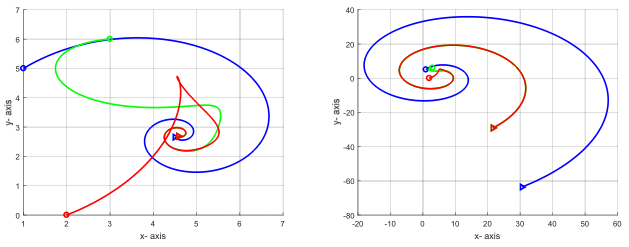
We consider the three agents under complete graph. But for a simplicity, we suppose that agent 11 has misaligned orientation as θ1\theta_{1} and agents 22 and 33 have the same misalignment angles as θ2=θ3\theta_{2}=\theta_{3}. Let us first consider θ1=π/1.9\theta_{1}=\pi/1.9 and θ2=θ3=−π/3\theta_{2}=\theta_{3}=-\pi/3. As shown in the left plots of Fig. 9, the agents converge to a common point although cos⁡θ1<0\cos\theta_{1}<0. But the converged point is not a average value of initial positions. Next, we slightly change θ1\theta_{1} as θ1=π/1.6\theta_{1}=\pi/1.6 with the same θ2=θ3=−π/3\theta_{2}=\theta_{3}=-\pi/3. The right plots of Fig. 9 show the trajectories of agents; but in this case, the agents diverge.
Refer to caption
Fig. 9: Example 33: Left: θ1=π/1.9\theta_{1}=\pi/1.9 and θ2=θ3=−π/3\theta_{2}=\theta_{3}=-\pi/3. Right: θ1=π/1.6\theta_{1}=\pi/1.6 and θ2=θ3=−π/3\theta_{2}=\theta_{3}=-\pi/3

V Discussions

As analyzed in Section III, even with orientation misalignments, the consensus could be achieved if −π/2<θi<π/2-\pi/2<\theta_{i}<\pi/2 and the consensus cannot be achieved if cos⁡θi<0,∀i∈𝒱\cos\theta_{i}<0,~\forall i\in\mathcal{V}. Also it was shown that the average consensus is no more ensured when some agents have the orientation misalignments. As remarked in Remark 1, when some agents have θi≤0\theta_{i}\leq 0 and some agents have θi≥0\theta_{i}\geq 0, it is difficult to develop a general result for consensus or non-consensus. With only two agents, as shown in Fig. 6, when θ1=π/2\theta_{1}=\pi/2 and θ2=−π/2\theta_{2}=-\pi/2, the agents diverge to infinity. Also with θ1=3​π/4\theta_{1}=3\pi/4 and θ2=−π/2\theta_{2}=-\pi/2, or θ1=3​π/4\theta_{1}=3\pi/4 and θ2=π/2\theta_{2}=\pi/2, agents diverge. But, with θ1=π/2+π/18\theta_{1}=\pi/2+\pi/18 and θ2=−π/18\theta_{2}=-\pi/18, a consensus was achieved. From these illustrations, it is now observed that when two control input vectors, i.e., −D⁡(θ1)​(p1−p2)-D(\theta_{1})(p_{1}-p_{2}) and −D⁡(θ2)​(p2−p1)-D(\theta_{2})(p_{2}-p_{1}), are directing opposite directions, the consensus is not achieved (also shown in Fig. 7). But, it is still hard to generalize the results. From the example with five agents, it was also confirmed that the consensus could be achieved if −π/2<θi<π/2-\pi/2<\theta_{i}<\pi/2 as illustrated in example 22-case 22 and example 22-case 33. But, in example 22-case 44, when agents 22 and 55 have θ2<0\theta_{2}<0 and θ5<0\theta_{5}<0, respectively, the consensus is not achieved. But, even when again 11 in example 22-case 55 has θ1<0\theta_{1}<0, the consensus is achieved, although in case 66, the consensus was not achieved. Thus, it is clear that the conditions developed in Theorem 3 are sufficient conditions.

Obviously the exact condition for a consensus can be achieved by examining eigenvalues of ℒo​u​t\mathcal{L}^{out} directly. Since the Laplacian matrix ℒo​u​t\mathcal{L}^{out} is a function of network topology and misaligned orientation angles θi\theta_{i}, it seems difficult to find the exact locations of eigenvalues (i.e., exact consensus condition) for general graphs. So, for general graphs, the regions defined by Theorem 3 seem to be best in terms of designing a consensus controller. For example, for two agents, the Laplacian matrix ℒo​u​t\mathcal{L}^{out} has eigenvalues as 0,0,(cos⁡θ1+cos⁡θ2)±j⁡(sin⁡θ1+sin⁡θ2)0,0,(\cos\theta_{1}+\cos\theta_{2})\pm j(\sin\theta_{1}+\sin\theta_{2}). Thus, a consensus is achieved if and only if 0<cos⁡θ1+cos⁡θ20<\cos\theta_{1}+\cos\theta_{2}, which is well coincident with the example 11 of Subsection IV-A. For three agents under a complete graph in Subsection IV-C, let us suppose that agent 11 has misaligned orientation as θ1\theta_{1} and agents 22 and 33 have the same misalignment angles as θ2=θ3\theta_{2}=\theta_{3}. Then, the eigenvalues of ℒo​u​t\mathcal{L}^{out} are 0,0,3cosθ2±3jsinθ2,2cosθ1+cosθ2±j(2sinθ1+sinθ2)0,0,3\cos\theta_{2}\pm 3j\sin\theta_{2},2\cos\theta_{1}+\cos\theta_{2}\pm j(2\sin\theta_{1}+\sin\theta_{2}). So, if and only if −π/2<θ2<π/2-\pi/2<\theta_{2}<\pi/2 and 2cosθ1+cosθ2>02\cos\theta_{1}+\cos\theta_{2}>0, the consensus could be achieved. This analysis is well matched to the simulations given in Subsection IV-C. However, it is hard to estimate the locations of eigenvalues of general graphs. Hence, it would be recommended to use the sufficient conditions developed in Theorem 3 for a designing purpose. That is, it is highly recommended to ensure the orientation misalignment errors as −π/2<θi<π/2-\pi/2<\theta_{i}<\pi/2.

VI Conclusion

This paper has presented a consensus problem under misalignments of orientations of agents. The three scenarios motivating the misalignment problems, depicted in Fig. 2, are misaligned orientation errors of local frames, biases in control directions or in sensing directions, and misalignment errors of virtually aligned coordinate frames. We have provided conditions for consensus and added some more analysis related with stability. The locations of eigenvalues have been roughly evaluated by using Gershgorin circle for a block matrix. From the existence of complex eigenvalues locating closely to the imaginary axis, the behaviors of agents are shown to be quite complicated. Also, it was illustrated that the converged consensus point could be quite away from the average of initial positions. Thus, it is highly required to have small misalignment errors; otherwise, the convergence time could be huge and the trajectories of agents become quite complicated. It seems difficult to find exact consensus condition for general graphs. Although we have presented only sufficient conditions, we believe that the conditions could be utilized for a design purpose nicely. In our future efforts, we would be focused on estimating the locations of eigenvalues more tightly in a distributed way.

References

  • [1] A. Jadbabaie, J. Lin, and A. S. Morse, “Coordination of groups of mobile autonomous agents using nearest neighbor rules,” IEEE Transactions on Automatic Control, vol. 48, no. 6, pp. 988–1001, 2003.
  • [2] J. A. Olfati-Saber, R. Fax and R. M. Murray, “Consensus and cooperation in networked multi-agent systems,” Proceedings of the IEEE, vol. 95, no. 1, pp. 215–233, 2007.
  • [3] T. Wongpiromsarn, K. You, and L. Xie, “A consensus approach to the assignment problem: Application to mobile sensor dispatch,” in Proc. of the 8th IEEE International Conference on Control and Automation. IEEE, June 2010, pp. 2024–2029.
  • [4] B.-Y. Kim and H.-S. Ahn, “Consensus-based coordination and control for building automation systems,” IEEE Trans. on Control Systems Technology, vol. 23, no. 1, pp. 364–371, 2015.
  • [5] Z. Zhang and M.-Y. Chow, “Convergence Analysis of the Incremental Cost Consensus Algorithm Under Different Communication Network Topologies in a Smart Grid,” IEEE Trans. Power Systems, vol. 27, no. 4, pp. 1761–1768, 2012.
  • [6] W. Ren, “Collective motion from consensus with cartesian coordinate coupling - Part I: Single-integrator kinematics,” in Proc. of the 47th IEEE Conference on Decision and Control. IEEE, Dec. 2008, pp. 1006–1011.
  • [7] ——, “Collective motion from consensus with cartesian coordinate coupling,” IEEE Trans. on Automatic Control, vol. 54, no. 6, pp. 1330–1335, 2009.
  • [8] J. L. Ramirez-Riberos, M. Pavone, E. Frazzoli, and D. W. Miller, “Distributed control of spacecraft formations via cyclic pursuit: Theory and experiments,” Journal of Guidance, Control, and Dynamics, vol. 33, no. 5, pp. 1655–1669, 2010.
  • [9] K.-K. Oh and H.-S. Ahn, “Formation control and network localization via orientation alignment,” IEEE Trans. on Automatic Control, vol. 59, no. 2, pp. 540–545, 2014.
  • [10] B.-H. Lee and H.-S. Ahn, “Distributed formation control via global orientation estimation,” Automatica, vol. 73, no. November, pp. 125–129, 2016.
  • [11] W. Ding, G. Yan, and Z. Lin, “Collective motions and formations under pursuit strategies on directed acyclic graphs,” Automatica, vol. 46, no. 1, pp. 174–181, 2010.
  • [12] B.-H. Lee and H.-S. Ahn, “Distributed estimation for the unknown orientation of the local reference frames in nn-dimensional,” in Proc. of the 14th International Conference on Control, Automation, Robotics & Vision, Nov., 2016, pp. 1–6.
  • [13] M. H. Trinh and H.-S. Ahn, “Theory and applications of matrix-weighted consensus,” arXiv:1703.00129v2 [math.OC], pp. 1–21, 2017.
  • [14] M. H. Trinh, C. V. Nguyen, Y.-H. Lim, and H.-S. Ahn, “Matrix-weighted consensus,” submitted for a publication, pp. –, 2017.
  • [15] D. G. Feingold and R. S. Varga, “Block diagonally dominant matrices and generalizations of the Gershgorin circle theorem,” Pacific Journal of Mathematics, vol. 12, no. 4, pp. 1241–1250, 1962.
  • [16] A. van der Sluis, “Gershgorln domains for partitioned matrices,” Linear Algebra and Its Applications, no. 26, pp. 265–280, 1979.