Cartan symmetries and global dynamical systems analysis in a higher-order modified teleparallel theory

L. Karpathopoulos Affiliation: Faculty of Physics, Department of Astronomy-Astrophysics-Mechanics University of Athens, Panepistemiopolis, Athens 157 83, Greece S. Basilakos Email: svasil@academyofathens.gr Affiliation: Academy of Athens, Research Center for Astronomy and Applied Mathematics, Soranou Efesiou 4, 11527, Athens, Greece G. Leon Email: genly.leon@ucn.cl Affiliation: Departamento de Matemáticas, Universidad Católica del Norte, Avda. Angamos 0610, Casilla 1280 Antofagasta, Chile A. Paliathanasis Email: anpaliat@phys.uoa.gr Affiliation: Instituto de Ciencias Físicas y Matemáticas, Universidad Austral de Chile, Valdivia, Chile Affiliation: Department of Mathematics and Natural Sciences, Core Curriculum Program, Prince Mohammad Bin Fahd University, Al Khobar 31952, Kingdom of Saudi Arabia Affiliation: Institute of Systems Science, Durban University of Technology, PO Box 1334, Durban 4000, Republic of South Africa M. Tsamparlis Email: mtsampa@phys.uoa.gr Affiliation: Faculty of Physics, Department of Astronomy-Astrophysics-Mechanics University of Athens, Panepistemiopolis, Athens 157 83, Greece

Abstract

In a higher-order modified teleparallel theory cosmological we present analytical cosmological solutions. In particular we determine forms of the unknown potential which drives the scalar field such that the field equations form a Liouville integrable system. For the determination of the conservation laws we apply the Cartan symmetries. Furthermore, inspired from our solutions, a toy model is studied and it is shown that it can describe the Supernova data, while at the same time introduces dark matter components in the Hubble function. When the extra matter source is a stiff fluid then we show how analytical solutions for Bianchi I universes can be constructed from our analysis. Finally, we perform a global dynamical analysis of the field equations by using variables different from that of the Hubble-normalization.

Keywords:

Cosmology; Symmetries; Cartan symmetries; Teleparallel; Critical Points

pacs

98.80.-k, 95.35.+d, 95.36.+x

August 24, 2026

I Introduction

A plethora of mechanisms has been introduced in order to explain the recent cosmological observations [1, 2, 3, 4]. In particular, the observed late-time acceleration of the universe has been attributed to a new matter source which has been called dark energy. Several models have been proposed for the dark energy among which scalar fields (quintessence, phantom fields, k-essence), fluids with time-varying equation of state parameters (Chaplygin gases) and the list goes on [6, 7, 8, 9, 10, 11, 12, 13, 14, 15, 16, 17, 18, 19, 20, 21, 22].

However, there is a large body of dark energy models which have geometric origin. In this class of scenarios the dark energy components correspond to the new degrees of freedom in the field equations, which are introduced by the modification of Einstein’s General Relativity. For instance, the introduction of quantum corrections in the Einstein’s General Relativity is performed with the use of higher-order invariants, such as polynomial terms involving the Ricci scalar, the Gauss Bonnet term and many others. These considerations have lead to the so called $f-$ theories, in which a function $f\left(X\right)$ is introduced in the Einstein-Hilbert action where $X$ is a geometric invariant [23, 24, 25, 26, 27, 28, 29, 30, 31, 32, 33, 34, 35, 36, 37, 38, 39, 40].

The Einstein-Hilbert action is not the unique action which provides the field equations of General Relativity. The Palatini formalism [41] and the teleparallel equivalent of GR (TEGR) [42] are two alternative variations which also under certain constraints lead again to General Relativity (for more details see [43, 44]). In TEGR the scalar invariant $T$ of the Weitzenböck connection is considered as the Lagrangian density of the field equations, while in the Palatini formalism the metric and the connection are varied independently.

In this article, we work in the context of the TEGR by considering a higher-order theory of gravity which introduces a scalar field with a noncanonical kinetic term as a dark-energy component [45, 46]¹¹ 1 In the following, with the term “canonical” scalar field we refer to the quintessence scalar field with a canonical kinetic term, that is, with Lagrangian $L_{\phi}=K-V$ .. Another well-known scalar field which is related with a modified theory is the field in the O’Hanlon theory which describes the geometrodynamic degrees of freedom in $f\left(R\right)-$ gravity. More details are given below.

We show that the field equations can be written with the use of a point-like Lagrangian. Which describes the classical analogue for the motion of two particles under an interaction between them, that is under the existence of an effective potential. The kinetic term of the point-like Lagrangian describes the degrees of freedom which concern the spacetime and the field, while the effective potential is related to those which drive the evolution of the new (noncanonical) scalar field.

We determine the special forms of this effective potential by requiring that the field equations are Liouville integrable and the solution of the Hamilton-Jacobi equation can be written in a closed-form expression. In order the latter to be possible, constraints on the action have to be determined which are equivalent to the existence of conservation laws. We derive these conservation laws and prove the Liouville integrability of the corresponding models by using the method of symmetries.

The symmetries, that is, the transformations which leave invariant a set of differential equations is a powerful method for the determination of conservation laws and exact solutions. The simplest type of symmetries are the Lie point symmetries which have been applied in various problems for the determination of new exact solutions either in the classical or at the quantum level [55, 56, 57, 58, 59, 60, 61]. For the gravitational models described by a point Lagrangian a special type of Lie point symmetries are those which in addition leave invariant the action integral. These Lie symmetries are called Noether symmetries which by means of Noether’s theorem allow the determination of conservation laws, for instance see [62, 63, 64, 65, 66, 67, 68, 69, 70, 71, 72, 73, 74, 75, 76, 77, 78, 79, 80]. In the present work we choose to work with the Cartan’s method in order to study the symmetries of our field equations. The Cartan symmetries are based on the invariance of the Cartan 1-form which is defined directly from the Lagrangian under point transformations with generators in the tangent bundle [81, 82, 83, 84]. It can be shown that for holonomic dynamical systems the Cartan symmetries are equivalent to the so-called generalized Noether symmetries [85], whereas for nonholonomic dynamical systems the situation is different [86].

Moreover, we perform a global dynamical analysis for that modified theory by using a different set of variables from the Hubble normalization. We see that the results of [45] are recovered; however new critical points are derived while we show that there can be physical processes which were not derived before. For instance, we show that it is possible the universe to pass from an accelerate phase to a decelerate phase and vice verca. Furthermore, we apply the results of the dynamical analysis to study the physical properties of the theories which followed from the symmetry analysis while the field equations are Liouville integrable. The plan of the paper is as follows.

In Section II, we present the cosmological model of our study. The field equations and the Lagrangian description in the minisuperspace approach are derived for a spatially flat Friedmann-Lemaître-Robertson-Walker (FLRW) universe with an ideal gas as an extra matter source. Furthermore, we consider the Lagrangian for the case of Bianchi I models and show that the field equations are reduced to that of FLRW when the ideal gas is a stiff fluid. In Section III we discuss briefly the Cartan formalism which we use in the determination of the conservation laws. In Section IV, we determine the specific forms of the unknown parameters of our model by requiring that the field equations admit Cartan symmetries. Moreover, the method of Hamilton-Jacobi is applied in order to reduce the field equations to a system of two first-order ordinary differential equations and when it is feasible to write the closed-form solution of the system. The dynamical system analysis is performed in Section V. We see that there is a specific potential for which the dimension of the dynamical system is reduced. The critical points are derived for all the possible families of theories as also their stability conditions. In Section VI we consider a closed-form solution from the previous section as a toy model and we perform a likelihood analysis with the SNIa data. We find that the model fits the SNIa data while at the same time the theory provides the dark matter components in the Hubble function. In Appendix A we give the critical points of the Hubble normalization and in Appendix B the critical points in the state space of observable quantities. In the Section VII, we investigate the evolution of the observables, the so called age parameter $\alpha=tH$ , the deceleration parameter $q$ , and the fractional energy of scalar field and Hubble-normalized kinetic term in a phase space. Imposing observational constraints on the current values of $\alpha_{0}=\alpha(\mathbf{y}_{0})$ , and the matter parameter $\Omega_{0}=1-\Omega_{\phi}(\mathbf{y}_{0})$ , restrict the location of the present state of the universe, $\mathbf{y}_{0}$ , in state space. Finally in Section VIII we draw our conclusions and discuss further possible extensions.

II Field equations

In the teleparallel equivalence of general relativity one introduces a non-holonomic frame by means of the functions $h_{i}^{\mu}$ so that the tangent vectors to the new coordinates are the vectors $e_{i}=h_{i}^{\mu}\left(x\right)\partial_{i}$ whose Lie bracket is $[e_{i},e_{j}]=c_{ij}^{...k}e_{k}$ where $c_{(ij)}^{...k}=0.$ In the nonholonomic coordinates the connection is not symmetric and it is given by the expression

\chi_{jk}^{i}=\{_{jk}^{i}\}+\frac{1}{2}g^{ir}(c_{rj,k}+c_{rk,j}-c_{ij,r})

(1)

where $c_{ijr}=g_{rk}c_{ij}^{...k}$ and $\{_{jk}^{i}\}$ is the standard Riemannian connection. In case the vectors $e_{i}$ are orthonormal then they form a vierbein field ${\mathbf{e}(x^{\mu})~}$ the metric becomes $\eta_{ij},~$ i.e. the Minkowski metric, while the connection coefficients reduce as follows

\chi_{jk}^{i}=\frac{1}{2}\eta^{ir}(c_{rj,k}+c_{rk,j}-c_{ij,r}).

(2)

In this case, the connection coefficients $\chi_{jk}^{i}$ are called the Ricci rotation coefficients, also known as the Weitzenböck connection [49]. Defining $\chi_{ijk}=\eta_{ir}\chi_{jk}^{r}$ we find that connection coefficients (2) have the property $\chi_{ijk}=-\chi_{jik};$ that is, they are antisymmetric in the first two indices.

The latter antisymmetric connection lead to the definition of the torsion tensor

T_{ijk}=\chi_{ijk}-\chi_{jik},

(3)

and subsequently the quantities are defined

K_{~~~\beta}^{\mu\nu}=-\frac{1}{2}({T^{\mu\nu}}_{\beta}-{T^{\nu\mu}}_{\beta}-{T_{\beta}}^{\mu\nu}),

(4)

The quantities $K_{~~~\beta}^{\mu\nu}~$ correspond to the contorsion tensor in the case of torsion.

Assuming that the non-holonomic frame is inherent in the structure of spacetime we have at our disposal $n^{2}$ new parameters $h_{i}^{\mu}$ which can be used for the definition of dark energy. We associate with dark energy the scalar field of geometric origin and noncanonical kinetic term with energy momentum tensor [45, 46]

4\pi Ge\mathcal{T}_{a}^{\left(\phi\right)}{}^{\lambda}=\frac{1}{2}e\left(h_{a}^{\sigma}\phi_{;\sigma}^{~~~;\lambda}-h_{a}^{\lambda}\phi^{;\mu\nu}g_{\mu\nu}\right)-e\phi_{;\mu}S_{a}{}^{\mu\lambda}-\frac{1}{4}eV\left(\phi\right)h_{a}^{\lambda}.

(5)

where the geometric object ${S_{\beta}}^{\mu\nu}$ is defined as

{S_{\beta}}^{\mu\nu}=\frac{1}{2}({K^{\mu\nu}}_{\beta}+\delta_{\beta}^{\mu}{T^{\theta\nu}}_{\theta}-\delta_{\beta}^{\nu}{T^{\theta\mu}}_{\theta}).

If $\mathcal{T}_{a}^{\left(m\right)}{}^{\lambda}$ is the energy momentum tensor which describes the usual matter source then the gravitational field equations of teleparallel gravity are of second-order and are given by the expression

eG_{a}^{\lambda}=4\pi Ge\left(\mathcal{T}_{a}^{\left(m\right)}{}^{\lambda}+\mathcal{T}_{a}^{\left(\phi\right)}{}^{\lambda}\right),

(6)

where $~G_{a}^{\lambda}$ is the Einstein-Tensor, where can be written with the use of teleparallel quantities as

eG_{i}^{\rho}\mathbf{=}2\left(e^{-1}\partial_{\mu}(ee_{i}^{\phantom{i}\rho}S_{\rho}{}^{\mu\nu})+e_{i}^{\phantom{i}\lambda}T^{\rho}{}_{\mu\lambda}S_{\rho}{}^{\nu\mu}+\frac{1}{4}e_{i}^{\phantom{i}\rho}T\right)

(7)

in which the scalar $T$ is defined as $T={S_{\beta}}^{\mu\nu}{T^{\beta}}_{\mu\nu}$ .

Furthermore, we assume that the additional matter source is minimally coupled with the scalar field the conservation equation (Bianchi identity) gives

\left(\mathcal{T}^{\left(m\right)a}{}^{\lambda}+\mathcal{T}^{\left(\phi\right)a}{}^{\lambda}\right)_{;\lambda}=0\rightarrow\left(\mathcal{T}^{\left(m\right)a}{}^{\lambda}\right)_{;\lambda}=0\text{ ~and ~}\left(\mathcal{T}^{\left(\phi\right)a}{}^{\lambda}\right)_{;\lambda}=0.

(8)

From (6) we observe that the field equations are written in the Einstein frame. Furthermore, as far as the origin of $\phi$ is concerned, that can have geometric origin and describe the higher-order terms of an extended $f-$ gravitational theory, for more details see [45, 46] and [47, 48].

A well known analogue is the Brans-Dicke scalar field [50]. Indeed the latter when the Brans-Dicke parameter is zero, which corresponds to the so-called O’Hanlon theory [51], is equivalent with the $f\left(R\right)$ -gravity in the metric formalism [24]. In particular the Brans-Dicke field attributes the higher-order derivatives of $f\left(R\right)$ gravity and the fourth-order theory can be written as second-order theory by increasing at the same time the number of degrees of freedom. Hence, in that explicitly analogue the energy momentum tensor (5) attributes the higher-order terms of a fourth-order $f-$ theory in which the invariant which is used for the modification of the Einstein-Hilbert action is the boundary term which relates the Ricci scalar and the invariant $T$ of the two connections in the holonomic and unholonomic frame, more details can be found in [45, 46].

II.1 Fourth-order theory of gravity

Let us now discuss the variational problem which describes the gravitational field equations (6), where $\mathcal{T}_{a}^{\left(\phi\right)}{}^{\lambda}$ is defined by (5).

Consider now the gravitational Action Integral to be

S\equiv\frac{1}{16\pi G}\int d^{4}xe\left[f(T,R+T)\right]+S_{m}\equiv\frac{1}{16\pi G}\int d^{4}xe\left[f(T,B)\right]+S_{m},

(9)

in which $e=\det(e_{\mu}^{i})=\sqrt{-g},~S_{m}$ is the Action Integral for the matter source and $B$ is the boundary term $B=2e_{\nu}^{-1}\partial_{\nu}\left(eT_{\rho}^{~\rho\nu}\right)$ which defined as

B=T+R

(10)

where $R$ is the Ricciscalar. Gravitational actions of the form of (9) have bee considered previously in [47] and [48]. As has been shown in [48] Action (9) generalize $f\left(T\right)$ -gravity while $f\left(R\right)$ gravity can be recovered. Moreover, because of the second-derivative terms which are included in the boundary $B$ , the resulting gravitational field equations of (9) are of fourth-order [45].

Indeed, variation with respect to the vierbein field provides the field equations [48]

	$\displaystyle 4\pi Ge\mathcal{T}_{a}^{\left(m\right)}{}^{\lambda}$	$\displaystyle=\frac{1}{2}ee_{a}^{\lambda}\left(f_{,B}\right)^{;\mu\nu}g_{\mu\nu}-\frac{1}{2}ee_{a}^{\sigma}\left(f_{,B}\right)_{;\sigma}^{~~~;\lambda}+\frac{1}{4}e\left(Bf_{,B}-\frac{1}{4}f\right)e_{a}^{\lambda}\,+(eS_{a}{}^{\mu\lambda})_{,\mu}f_{,T}$
		$\displaystyle~\ ~+e\left((f_{,B})_{,\mu}+(f_{,T})_{,\mu}\right)S_{a}{}^{\mu\lambda}~-ef_{,T}T^{\sigma}{}_{\mu a}S_{\sigma}{}^{\lambda\mu},$		(11)

where $\mathcal{T}_{a}^{\left(m\right)}{}^{\lambda}$ is the energy-momentum tensor of the matter source.

We follow the analysis described in [46] and we rewrite the field equations (11) as follows

eG_{a}^{\lambda}=G_{eff}e\left(\mathcal{T}_{a}^{\left(m\right)}{}^{\lambda}+\mathcal{T}_{a}^{\left(DE\right)}{}^{\lambda}\right),

(12)

in which $G_{eff}=\frac{4\pi G}{f_{,T}}$ denotes the effective varying “gravitational constant”, and the energy-momentum tensor $\mathcal{T}_{a}^{\left(DE\right)}{}^{\lambda}$ is defined as [46]

	$\displaystyle 4\pi Ge\mathcal{T}_{a}^{\left(DE\right)}{}^{\lambda}$	$\displaystyle=-\left[\frac{1}{4}\left(Tf_{,T}-f\right)eh_{a}^{\lambda}+e(f_{,T})_{,\mu}S_{a}{}^{\mu\lambda}\right]+$		(13)
		$\displaystyle-\left[e(f_{,B})_{,\mu}S_{a}{}^{\mu\lambda}-\frac{1}{2}e\left(e_{a}^{\sigma}\left(f_{,B}\right)_{;\sigma}^{~~~;\lambda}-e_{a}^{\lambda}\left(f_{,B}\right)^{;\mu\nu}g_{\mu\nu}\right)+\frac{1}{4}eBe_{a}^{\lambda}f_{,B}\right],$

which includes the fourth-order derivatives of the theory.

The latter energy-momentum tensor can be seen as the geometric dark-energy source which drives the dynamics of the universe in order to explain the acceleration phases of the universe, for discussions on geometric dark-energy models see [52, 53] and references therein.

As we saw, in general the “gravitational constant” is varying with a function of $f^{-1}\left(T\right)$ . However, if we assume now that $f\left(T,B\right)$ is a linear function on $T$ , that is $f_{,T}=const$ , that is $f\left(T,B\right)=T+F\left(B\right)$ , then we derive that $G_{eff}=4\pi G$ . That simplest scenario was studied for the first time in [45].

Moreover, in $T+F\left(B\right)$ theory, the geometric dark-energy momentum tensor (13) is simplified as [46]

4\pi Ge\mathcal{T}_{a}^{\left(B\right)}{}^{\lambda}=-\left[e(F_{,BB})B_{;\mu}S_{a}{}^{\mu\lambda}-\frac{1}{2}e\left(e_{a}^{\sigma}\left(F_{,B}\right)_{;\sigma}^{~~~;\lambda}-e_{a}^{\lambda}\left(F_{,B}\right)^{;\mu\nu}g_{\mu\nu}\right)+\frac{1}{4}e\left(BF_{,B}-F\right)e_{a}^{\lambda}\right]

(14)

or equivalently is written in the form of (5) where now the field $\phi$ describes second-order terms, that is, $\phi=F\left(B\right)_{,B}$ , with $V\left(\phi\right)=$ $\left(F-BF_{,B}\right).$ Therefore, the geometric origin for the field $\phi$ is obvious. However, because $G_{eff}=4\pi G=const$ . we can say that the field $\phi$ is defined in the Einstein frame, in contrary to the Scalar-tensor theories defined in the Jordan frame.

That specific form of $f\left(T,B\right)$ -theory it is possible to provides cosmological eras which describes the two acceleration phases of our universe, the inflation and the late-time acceleration [45], while an epoch where the geometric dark-energy fluid mimics an ideal gas can be recovered [46]. Another special property of the $T+F\left(B\right)$ theory is that when $B$ is constant, then the gravitational field equations (11) are those of General Relativity with cosmological constant.

Furthermore, as we shall below for the $T+F\left(B\right)~$ theory in a FLRW and in a Bianchi I background it is possible to describe the field equations by using the minisuperspace approach. Such a description is important in order to apply mathematical methods from analytical mechanics and derive analytical solutions for the field equations.

II.2 FLRW

In the case of an isotropic and homogeneous spacetime with zero spatial curvature the line element is

ds^{2}=-N^{2}\left(t\right)dt^{2}+a^{2}\left(t\right)\left(dx^{2}+dy^{2}+dz^{2}\right),

(15)

where $a\left(t\right)$ is the scale-factor of the three dimensional Euclidean space and $N\left(t\right)$ is the lapse function. The commoving observers are $u^{\mu}=\frac{1}{N}\delta_{t}^{\mu}.$ For the vierbein we considered the quantities

h_{\mu}^{i}(t)=\mathrm{diag}\left(N\left(t\right),a\left(t\right),a\left(t\right),a\left(t\right)\right).

(16)

We assume that the matter source for the comoving observer is that of a perfect fluid with matter density $\rho_{m}$ and pressure $p_{m};$ the energy momentum tensor for the comoving observers is given by the expression

\mathcal{T}_{a\lambda}^{\left(m\right)}{}=\left(\rho_{m}+p_{m}\right)u_{a}u_{\lambda}+p_{m}g_{\alpha\lambda},

(17)

while the Bianchi identity provides

\dot{\rho}_{m}+3\frac{\dot{a}}{a}\left(\rho_{m}+p_{m}\right)=0.

(18)

Furthermore, we consider that the equation of state parameter of the matter source is constant, such that $p_{m}=w_{m}\rho_{m}$ , and we impose the restriction $w_{m}\in[-1,1]$ ; hence from (18) it follows $\rho_{m}\left(t\right)=\rho_{m0}a\left(t\right)^{-3\left(w_{m}+1\right)}.$

For the frame (16) from expression (5) we calculate that the nonzero components of the energy momentum tensor $\mathcal{T}_{a}^{\left(\phi\right)}{}^{\lambda}$ are

4\pi Ge\mathcal{T}_{t}^{\left(\phi\right)}{}^{t}=-\left(3\frac{\dot{a}\dot{\phi}}{aN^{2}}+\frac{1}{2}V\left(\phi\right)\right)

(19)

and

4\pi Ge\mathcal{T}_{x}^{\left(\phi\right)}{}^{x}=4\pi Ge\mathcal{T}_{y}^{\left(\phi\right)}{}^{y}=4\pi Ge\mathcal{T}_{z}^{\left(\phi\right)}{}^{z}=-\left(\frac{\ddot{\phi}}{N^{2}}-\frac{\dot{\phi}\dot{N}}{N^{3}}+\frac{1}{2}V\left(\phi\right)\right).

(20)

The nonzero components of the Einstein tensor are calculated to be

G_{0}^{0}=-3\left(\frac{\dot{a}}{aN}\right)^{2}~,~G_{x}^{x}=G_{y}^{y}=G_{z}^{z}=-\left(2\frac{\ddot{a}}{aN^{2}}+\left(\frac{\dot{a}}{aN}\right)^{2}-2\frac{\dot{a}\dot{N}}{aN^{3}}\right).

(21)

From expressions (19) and (20) for the comoving observer $u^{\mu}$ we compute the energy density and the pressure of the field $\phi$ as follows

\rho_{\phi}=3\frac{\dot{a}\dot{\phi}}{aN^{2}}+\frac{1}{2}V\left(\phi\right)~,~p_{\phi}=-\left(\frac{\ddot{\phi}}{N^{2}}-\frac{\dot{\phi}\dot{N}}{N^{3}}+\frac{1}{2}V\left(\phi\right)\right)

and the equation of state parameter is

w_{DE}=\frac{p_{\phi}}{\rho_{\phi}}=-\frac{N\ddot{\phi}-\dot{\phi}\dot{N}+\frac{1}{2}N^{3}V\left(\phi\right)}{3N\frac{\dot{a}}{a}\dot{\phi}+\frac{1}{2}N^{3}V\left(\phi\right)}.

(22)

Finally, the conservation equation (8) for the field $\phi$ gives

\frac{1}{6}V_{,\phi}+\frac{\ddot{a}}{\dot{a}N^{2}}+2\left(\frac{\dot{a}}{aN}\right)^{2}-\frac{\dot{a}\dot{N}}{aN^{3}}=0.

(23)

In the case where the lapse function $N\left(t\right)$ is constant, i.e. $N\left(t\right)=1$ , the gravitational field equations (6) take the following simple form

3H^{2}=3H\dot{\phi}+\frac{1}{2}V\left(\phi\right)+\rho_{m},

(24)

2\dot{H}+3H^{2}=\ddot{\phi}+\frac{1}{2}V\left(\phi\right)-p_{m},

(25)

and the constraint equations are

\frac{1}{6}V_{,\phi}+\dot{H}+3H^{2}=0,

(26)

\dot{\rho}_{m}+3H\left(\rho_{m}+p_{m}\right)=0,

(27)

where $H=\frac{\dot{a}}{a}$ is the Hubble function. Recall, that for arbitrary lapse function the Hubble function is defined as $H\left(t\right)=\frac{\dot{a}}{aN}$ .

II.3 Minisuperspace description

Following [45] we construct a point-like Lagrange so that the field equations are derived from the Hamiltonian variational principle of least action. The corresponding Lagrange function is

\mathcal{L}\left(N,a,\dot{a},\phi,\dot{\phi}\right)=-\frac{6}{N}a\dot{a}^{2}+\frac{6}{N}a^{2}\dot{a}\dot{\phi}-Na^{3}V\left(\phi\right)-2\rho_{m0}Na^{-3w_{m}},

(28)

which is a singular Lagrangian in the sense that the Hessian matrix $\frac{\partial^{2}\mathcal{L}}{\partial\dot{a}\partial\dot{\phi}}$ vanishes. This is to be expected because the field equations admit second-order derivatives of the variables $\left(a,\phi\right)$ , while the variable $N$ provides the constraint equation $G_{0}^{0}=T_{0}^{0}$ .

Without loss of generality we may consider that $N=N\left(a,\phi\right).$ Then the field equations describe the evolution of a canonical particle moving in a two dimensional space under the action of an effective potential. From the kinetic term of (28) we construct the minisuperspace metric $\chi_{ij}=\frac{\partial^{2}\mathcal{L}}{\partial\dot{a}\partial\dot{\phi}}=\frac{\partial^{2}L}{\partial\dot{q}^{i}\partial\dot{q}^{j}}$ , while the effective potential is

V_{eff}\left(a,\phi\right)=Na^{3}V\left(\phi\right)+2\rho_{m0}Na^{-3w_{m}}.

(29)

Finally the constraint equation (24) is the Hamiltonian invariant, because the field equations are autonomous, which has a specific value. Specifically, because of the constraint the Hamiltonian vanishes.

In the case in which $w_{m}=1$ the matter source is called stiff fluid of the spacetime can it can be attributed to an extra degree of freedom, that is, it corresponds to additional free scalar fields. That property is used to extend our analysis in the case of the vacuum Bianchi I model.

In the following, we derive the field equations for the case of the vacuum Bianchi I universe and we show explicity how Lagrangian (28) describes the field equations for the Bianchi I universe when $\rho_{m0}$ is related with the integration constants for the anisotropic parameters of the inhomogeneous spacetime.

II.4 Bianchi I

In Bianchi I spacetime the line element in the Misner variables is written as follows,

ds^{2}=-N^{2}\left(t\right)dt^{2}+a^{2}\left(t\right)\left(e^{-2\beta_{+}\left(t\right)}dx^{2}+e^{\beta_{+}\left(t\right)+\sqrt{3}\beta_{-}\left(t\right)}dy^{2}+e^{\beta_{+}\left(t\right)-\sqrt{3}\beta_{-}\left(t\right)}dy^{2}\right).

(30)

The latter line element admits a three dimensional abelian Killing group. Functions $\beta_{+},~\beta_{-}$ are called the anisotropic parameters [54].

We consider the diagonal frame

h_{\mu}^{i}(t)=\mathrm{diag}(N\left(t\right),a(t)e^{-\beta_{+}\left(t\right)},a(t)e^{\frac{1}{2}\left(\beta_{+}\left(t\right)+\sqrt{3}\beta_{-}\left(t\right)\right)},a(t)e^{\frac{1}{2}\left(\beta_{+}\left(t\right)-\sqrt{3}\beta_{-}\left(t\right)\right)}),

(31)

from where we calculate the invariant

T=\left(-6\left(\frac{\dot{a}}{aN}\right)^{2}+\frac{3}{2}\left(\frac{\dot{\beta}_{+}}{N}\right)^{2}+\frac{3}{2}\left(\frac{\dot{\beta}_{-}}{N}\right)^{2}\right)

(32)

and the corresponding Lagrangian of the field equations (6) in the case of the vacuum is derived to be

\mathcal{L}\left(N,a,\dot{a},\phi,\dot{\phi}\right)=-\frac{6}{N}a\dot{a}^{2}+\frac{3}{2}Na^{-3}\left(\frac{a^{3}\dot{\beta}_{+}}{N}\right)^{2}+\frac{3}{2}Na^{-3}\left(\frac{a^{3}\dot{\beta}_{-}}{N}\right)^{2}+\frac{6}{N}a^{2}\dot{a}\dot{\phi}-Na^{3}V\left(\phi\right).

(33)

For the Lagrangian (33) we observe that the quantities

\Phi_{+}=\left(\frac{a^{3}\dot{\beta}_{+}}{N}\right)\text{ and }\Phi_{-}=\left(\frac{a^{3}\dot{\beta}_{-}}{N}\right)

(34)

are conservation laws, that is $\frac{d\Phi_{\pm}}{dt}=0$ , which means that with the application of the conservation laws the dynamical system can be reduced to that of FLRW Lagrangian (28) where $\rho_{m0}=\rho_{m0}\left(\Phi_{+},\Phi_{-}\right)$ and $w_{m}=1$ .

III Cartan formalism and symmetries

In this section we briefly discuss the method of Cartan for the study of symmetries of Lagrange equations and consequently of the admitted conservation laws. Because we are interested on systems of differential equations of second-order we consider Lagrangians of the form $\mathcal{L}=\mathcal{L}\left(t,x^{j},\dot{x}^{j}\right)$ where $t$ is the independent variable, $x^{i}\left(t\right)$ are the dependent variables and a dot denotes total derivative with respect to $t$ .

From the variation of the action $S=\int Ldt$ , follows the Euler Lagrange equations $E_{L}\left(L\right)=0$ where $E_{\mathcal{L}}=\frac{d}{dt}\frac{\partial}{\partial\dot{x}^{i}}-\frac{\partial}{\partial x^{i}}~$ is the Euler-operator. Assume that the field equations are written in the form

\ddot{x}^{i}=\Lambda^{i}\left(t,x^{j},u^{j}\right)

where $u^{i}=\dot{x}^{j}.$ We define the associated vector field $A$ to the Lagrangian system, called the Hamiltonian flow, as follows

A=\partial_{t}+u^{i}\partial_{i}+\Lambda^{i}\partial_{u^{i}}

where $\Lambda^{i}=\Lambda^{i}\left(t,x^{j},u^{j}\right)$ is defined by the condition

\frac{\partial^{2}\mathcal{L}}{\partial u^{i}\partial u^{j}}\Lambda^{j}=\frac{\partial\mathcal{L}}{\partial x^{i}}-\frac{\partial^{2}\mathcal{L}}{\partial u^{i}\partial x^{j}}u^{j}-\frac{\partial^{2}\mathcal{L}}{\partial u^{i}\partial t}.

(35)

In the cotangent space we consider the basis

\left(de^{1},de^{2},de^{3}\right)=\left(dx^{i}-u^{i}dt~,~du^{i}-\Lambda^{i}dt~,~dt\right),

(36)

We note that the vector field $A=\partial_{t}+u^{i}\partial_{i}+\Lambda^{i}\partial_{u^{i}}$ has the property²² 2 The operator $i_{A}$ denotes the left-hook or antiderivation with respect the Hamiltonian flow. $i_{A}\left(de^{1},de^{2},de^{3}\right)=\left(0,0,0\right).$ It is easy to show that every closed differential form $df$ in that basis is expressed as follows

df=\frac{\partial f}{\partial x^{i}}\left(dx^{i}-u^{i}dt\right)+\frac{\partial f}{\partial u^{i}}\left(du^{i}-\Lambda^{i}dt\right)+A\left(f\right)dt.

(37)

We introduce the Cartan 1-form $\theta$ [84]

\theta=\mathcal{L}dt+\frac{\partial\mathcal{L}}{\partial u^{i}}\left(dx^{i}-u^{i}dt\right).

(38)

$\theta$ is the the pullback under the Legendre transform of the fundamental one form $u_{i}dx^{i}-Hdt$ in Hamiltonian mechanics where $H\$ is the Hamiltonian. In terms of $\theta$ the equations of motions are

i_{A}\left(d\theta\right)=0.

(39)

$d\theta$ is a 2-form called the second Cartan form which in basis (36) is expressed as follows

d\theta=\frac{\partial\mathcal{L}}{\partial u^{i}\partial u^{j}}\left[\left(dx^{j}-u^{j}dt\right)\curlywedge\left(dx^{i}-u^{i}dt\right)+\left(du^{i}-\Lambda^{i}dt\right)\curlywedge\left(dx^{j}-u^{j}dt\right)\right],

(40)

where $\curlywedge$ denotes the wedge product.

Therefore, if there exists a closed-form $f$ , such that two Cartan one forms are related such that

\bar{\theta}-\theta=df,

(41)

then $\theta$ and $\bar{\theta}$ describe the same field equations, because by definition $d\left(\bar{\theta}-\theta\right)=d^{2}f\equiv 0$ .

In the tangent space consider the point transformation

\left(\bar{t},\bar{x}^{i},\bar{u}^{i}\right)=\left(t+\varepsilon\xi\left(t,x^{j},u^{j}\right),x^{i}+\varepsilon\eta^{i}\left(t,x^{j},u^{j}\right),u^{i}+\varepsilon\zeta^{i}\left(t,x^{j},u^{j}\right)\right)

(42)

generated by the vector field

X=\xi\frac{\partial}{\partial t}+\eta^{i}\frac{\partial}{\partial x^{i}}+\zeta^{i}\frac{\partial}{\partial u^{i}}.

(43)

We say that $X$ is a Cartan symmetry of the Lagrangian $L$ if

L_{X}\left(d\theta\right)=0

(44)

where $L_{X}$ denotes the Lie derivative with respect to the vector field $X$ .

Because $L_{X}\left(d\theta\right)=d\left(L_{X}\theta\right)$ we conclude that the condition for a Cartan-symmetry is [82]

L_{X}\left(d\theta\right)=0\text{ or }L_{X}\left(\theta\right)=df.

(45)

where $f$ is a function. The latter condition describes nothing else than Noether’s first theorem in the cotangent space while it is clear that $f$ is a boundary term and inaccurately it is characterized as a gauged function. Furthermore using the identity $L_{X}\theta=i_{X}\left(d\theta\right)+d\left(i_{X}\theta\right)$ we find that if $X$ is a Cartan symmetry then $L_{X}\theta=0$ and

i_{A}d\left(f-i_{X}\theta\right)=0

(46)

which means that the quantity $\left(f-i_{X}\theta\right)$ is conserved. Expression (46) describes Noether’s second theorem. Finally, if $X$ is a Cartan symmetry then $i_{\left[A,X\right]}d\theta=i_{A}L_{X}d\theta-L_{X}\left(i_{A}d\theta\right)$ which means that $L_{X}\left(i_{A}d\theta\right)=0$ . The latter condition implies that Cartan symmetries leave invariant the field equations (as expected) and form a subalgebra of the Lie symmetries of the dynamical system.

III.1 Symmetries for point-like Lagrangians

For Lagrangian $\mathcal{L}=\frac{1}{2}g_{ij}\left(x^{j}\right)u^{i}u^{j}-V\left(x^{k}\right)$ the Cartan one-form is calculated to be

\theta=\left(\frac{1}{2}g_{ij}u^{i}u^{j}-V\right)dt+g_{ij}u^{j}\left(dx^{i}-u^{i}dt\right)

(47)

We consider the vector field $X=\xi\partial_{t}+\eta^{i}\partial_{i}+\zeta^{i}\partial_{u^{i}}$ and require it to be a Cartan symmetry. However, since $X$ is also a Lie symmetry it follows that $\zeta^{i}$ is not independent but it can expressed explicitly in terms of $\xi,~\eta^{i}$ and their derivatives³³ 3 This is possible only for holonomic dynamical systems.

\zeta^{i}=\eta_{,t}^{i}+u^{k}\eta_{,k}^{i}+\Lambda^{k}\eta_{,u^{k}}^{i}-u^{i}\left(\xi_{,t}+u^{k}\xi_{,k}+\Lambda^{k}\xi_{,u^{k}}\right).

(48)

From the symmetry condition (45) it follows

	$\displaystyle L_{X}\theta$	$\displaystyle=\left[g_{ij,k}\eta^{k}u^{j}+g_{ij}\zeta^{j}\right]dx^{i}+g_{ij}u^{j}\eta_{,k}^{i}dx^{k}-\frac{1}{2}g_{ij}u^{i}u^{j}\xi_{,k}dx^{k}+$
		$\displaystyle+\left[-g_{ij}u^{i}\zeta^{j}-\frac{1}{2}g_{ij,k}\eta^{k}u^{i}u^{j}+g_{ij}u^{j}\eta_{,t}^{i}-\frac{1}{2}g_{ij}u^{i}u^{j}\xi_{,t}-\eta^{k}V_{k}\right]dt+$
		$\displaystyle+\left[g_{ij}u^{j}\eta_{,u^{k}}^{i}-\frac{1}{2}g_{ij}u^{i}u^{j}\xi_{,u^{k}}^{i}\right]du^{k}$
		$\displaystyle=f_{,t}dt+f_{,i}dx^{i}+f_{,u^{k}}du^{k}$

from where we find the following set of equations

$\displaystyle\left[g_{ij,k}\eta^{k}u^{j}+g_{ij}\zeta^{j}\right]\delta_{r}^{i}+g_{ij}u^{j}\eta_{,k}^{i}\delta_{r}^{k}-\frac{1}{2}g_{ij}u^{i}u^{j}\xi_{,k}\delta_{r}^{k}-f_{,r}$	$\displaystyle=0.$	(49)
$\displaystyle-g_{ij}u^{i}\zeta^{j}-\frac{1}{2}g_{ij,k}\eta^{k}u^{i}u^{j}+g_{ij}u^{j}\eta_{,t}^{i}-\frac{1}{2}g_{ij}u^{i}u^{j}\xi_{,t}-f_{,t}-\eta^{k}V_{k}$	$\displaystyle=0.$	(50)
$\displaystyle g_{ij}u^{j}\eta_{,u^{k}}^{i}-\frac{1}{2}g_{ij}u^{i}u^{j}\xi_{,u^{k}}^{i}-f_{,u^{k}}$	$\displaystyle=0.$	(51)

Specific forms of the functions $\xi$ and $\eta^{i}$ reduce the above system to various special forms.

III.1.1 Point transformations

In this case both $\xi$ and $\eta$ are independent of $u^{i}$ and the resulting symmetry conditions become

	$\displaystyle V_{,k}\eta^{k}+V\xi_{,t}+f_{,t}$	$\displaystyle=0~~,~~\eta_{,t}^{i}g_{ij}-\xi_{,j}V-f_{,j}=0$		(52)
	$\displaystyle L_{\eta}g_{ij}-\xi_{,t}g_{ij}$	$\displaystyle=0~~,~~\xi_{,i}=0~~,~~f_{,u^{k}}=0$		(53)

whose general solution can be found in [87]. Finally, the corresponding conservation law is linear in the velocity $u^{i}$ .

III.1.2 Higher-order symmetries

When $\xi$ and $\eta$ are functions $u^{i}$ these symmetries are called higher-order symmetries. A particular class of higher order symmetries are the contact symmetries in which $\xi$ and $\eta^{i}$ are linear functions of $u^{i}.$ In this case it can be shown that without loss of generality one can set $\xi=0$ and $\eta^{i}=K_{~j}^{i}\left(t,x^{k}\right)u^{j}$ . If this is done then the symmetry conditions take the simple form

	$\displaystyle K_{\left(ij\right),t}$	$\displaystyle=0~~,~~K_{(is;j)}=0$		(54)
	$\displaystyle g_{ij}V^{k}K_{k}^{j}+f_{,i}$	$\displaystyle=0~~,~~f_{,t}=0~,~~f_{,u^{k}}=0.$		(55)

In a similar way the symmetry conditions can be derived for other dependence of $\eta^{i}$ on $u^{i}$ . In general it is easy to show that if $\eta^{i}$ is a polynomial of rank $n$ on $u^{i}$ then the corresponding symmetry conditions are polynomials of rank $\left(n+1\right)$ on $u^{i}$ .

	$\displaystyle K_{\left(irs;j\right)}$	$\displaystyle=0~~,~~K_{\left(irs\right),t}=0~~$		(56)
	$\displaystyle V^{k}K_{(iks)}$	$\displaystyle=0~~,~~f=0.$		(57)

While the point symmetries form a Lie algebra for the higher-order symmetries there are some differences. For instance, if $K_{\left(1\right)},~K_{\left(2\right)}$ are second-rank tensor which produce two contact symmetries with boundary terms $f_{\left(1\right)}$ and $f_{\left(2\right)}$ then it follows that

\left[K_{\left(1\right)},K_{\left(2\right)}\right]_{SN}\left(V_{k}\right)+\left[f_{\left(1\right);i},f_{\left(2\right);j}\right]=K^{ijk}V_{k}+\left[f_{\left(1\right);i},f_{\left(2\right);j}\right]

(58)

where $\left[K_{\left(1\right)},K_{\left(2\right)}\right]_{SN}$ denotes the Schouten-Nijenhuis Bracket. It follows that $K^{ijk}$ produces a quadratic higher-order symmetry if and only if $\left[f_{\left(1\right);i},f_{\left(2\right);j}\right]=0$ . Therefore the commutator of two higher order symmetries produces a higher-order symmetry of higher rank.

In the special case that the boundary terms for contact or higher symmetries are zero, that is $f_{\left(1\right)}=f_{\left(2\right)}=0~$ , or for noncontact higher-order symmetries, it follows that if the Lagrangian $\mathcal{L}$ admits the conserved quantities $I_{A}$ , $I_{B}$ , defined as

I_{A}=K_{ij_{1}...j_{a}}u^{i}u^{j_{1}}...u^{j_{a}}~,~I_{B}=T_{ij_{1}...j_{b}}u^{i}u^{j_{1}}...u^{j_{b}}

(59)

with $a,b>1,$ then also the quantity

I_{S}=S_{ij_{1}...j_{c}}u^{i}u^{j_{1}}...u^{j_{c}}~,~c=a+b-1

(60)

is a conserved quantity, where $\mathbf{S\equiv}\left[\mathbf{K,T}\right]_{SN}$ .

In the following Section, we continue with the determination of the unknown parameters of the field equations (6) so that Cartan symmetries are admitted which provide conserved quantities sufficient to prove the integrability of the field equations and when it is feasible to write the solution in closed-form.

IV Symmetries and analytic Solutions

In the Lagrangian of the field equations (28) without loss of generality we consider that $N\left(t\right)=a^{3w_{m}}$ . With that selection the fluid term has been absorbed in the minisuperspace which simplifies our calculations. Then the Cartan 1-form which describes the field equations is calculated to be

	$\displaystyle\theta$	$\displaystyle=\left(-6a^{1-3w_{m}}\dot{a}^{2}+6a^{2-3w_{m}}\dot{a}\dot{\phi}-a^{3\left(1+w_{m}\right)}V\left(\phi\right)+2\rho_{m0}\right)dt+$
		$\displaystyle+\left(-12a^{1-3w_{m}}\dot{a}+6a^{2-3w_{m}}\dot{\phi}\right)\left(da-\dot{a}dt\right)+\left(6a^{2-3w_{m}}\dot{a}\right)\left(d\phi-\dot{\phi}dt\right),$		(61)

and the corresponding Hamiltonian flow is

	$\displaystyle A$	$\displaystyle=\frac{\partial}{\partial t}+\dot{a}\frac{\partial}{\partial a}+\dot{\phi}\frac{\partial}{\partial\phi}+\left(\left(3w-2\right)\frac{\dot{a}^{2}}{a}+\frac{a^{1+6w}}{6}V_{,\phi}\right)\partial_{\dot{a}}+$
		$\displaystyle~~~~~~~~~+\left(3\left(w-1\right)\left(\frac{\dot{a}}{a}\right)^{2}+\frac{a^{6w}(3\left(w+1\right)V+2V_{,\phi})}{6}\right)\partial_{\dot{\phi}}.$		(62)

The field equations have four degrees of freedom $\left(a,\dot{a},\phi,\dot{\phi}\right)$ , with the constraint equation, the conservation law of “energy” to be zero, that is the Hamiltonian $H=0$ . Hence, the determination of a second conservation law is sufficient to prove the integrability of the field equations, as defined by Liouville⁴⁴ 4 In the following, with the term integrability we mean Liouville integrability.. Recall, that the second conservation law should be linearly independent from the Hamiltonian and in involution.

Another important question is which kind of symmetries have to be used for the determination of integrable systems. For instance there are different systems which admit point symmetries and other higher-order symmetries. However these two sets of systems are not independent and the systems which admit point symmetries are included in the systems which admit higher-order symmetries. This is easy to show by using the inverse problem to construct the symmetry vector from the conservation law.

The inverse problem says that if $\Phi$ is a constant of motion for a system with Cartan 1-form $\theta$ , then there exists a vector field $X$ such that $L_{X}\theta=d\left(F+i_{X}\theta\right)$ , that is, $X$ is a Cartan symmetry, while any vector field $Y=X+\lambda A$ is also a Cartan symmetry which produces the same conservation law. Hence, all point symmetries generate conservation laws linear in the velocities. However any function of a conservation law is also a conservation law which means that if $\Phi_{P}$ is a conservation law generated by a point symmetry then $\Phi_{C}=\left(\Phi_{P}\right)^{2}$ is a conservation law associated with a contact symmetry. Hence, we prefer to work with the higher-order symmetries and specifically with the Cartan symmetries generated by contact transformations. We omit the calculations for the derivation of Cartan symmetries and their corresponding conservation laws and we continue with the direct presentation of the results.

IV.1 Classification of Cartan symmetries

We find that there are some differences between the potentials and the conservation laws for $w_{m}\neq 1$ and $w_{m}=1$ .

IV.1.1 Non stiff fluid $w_{m}\neq 1$

In particular for $w_{m}\neq 1$ we find that the scalar field potentials for which the field equations admit Cartan symmetries generated by the contact transformations are the following

V_{A}\left(\phi\right)=V_{1}\phi+V_{0},

(63)

V_{B}\left(\phi\right)=V_{1}e^{-3(w_{m}+1)\phi}+V_{2}e^{-6w_{m}\phi}.

(64)

and

V_{C}\left(\phi\right)=V_{1}e^{-3\left(1+w_{m}\right)\phi}+V_{2}e^{-\frac{3}{2}\left(3+w_{m}\right)}

(65)

The conservation law which corresponds to the potential $V_{A}\left(\phi\right)$ is

I_{A}=a^{4-6w_{m}}\dot{a}^{2}+\frac{V_{1}}{18}a^{6}

(66)

while for the potential $V_{B}\left(\phi\right)~$ the additional conservation law is

I_{B}=\left(\frac{\dot{a}-a\dot{\phi}}{a}\right)^{2}+\frac{(w_{m}-1)}{6w_{m}}V_{2}\left(ae^{-\phi}\right)^{6w_{m}}~\text{for}~w_{m}\neq 0,

(67)

I_{B}^{0}=\left(\frac{\dot{a}}{a}-\dot{\phi}\right)^{2}-V_{2}\left(\ln a-\phi\right)~\text{\ for}~w_{m}=0.

(68)

For the potential $V_{C}\left(\phi\right)~$ the extra conservation law is

$\displaystyle I_{C}$	$\displaystyle=a^{1-3w_{m}}\left(2+3\left(1-w_{m}\right)\left(\phi-\ln a\right)\right)\dot{a}^{2}-3a^{2-3w_{m}}\left(1+\left(1-w_{m}\right)\left(\phi-\ln a\right)\right)\dot{a}\dot{\phi}+$
	$\displaystyle~+a^{3\left(1-w_{m}\right)}\dot{\phi}^{2}+\frac{V_{1}}{6\left(1+w_{m}\right)}\left(2+3\left(w_{m}^{2}-1\right)\left(\ln a-\phi\right)\right)a^{3\left(1+w_{m}\right)}e^{-3\left(1+w_{m}\right)\phi}+$
	$\displaystyle+\frac{V_{2}}{6}\left(1+3\left(1-w_{m}\right)\left(\phi-\ln a\right)\right)a^{3\left(1+w_{m}\right)}e^{-\frac{3}{2}\left(3+w_{m}\right)\phi}.$	(69)

IV.1.2 Stiff fluid $w_{m}=1$

When $w_{m}=1$ , that is, the matter source is that of stiff fluid the symmetry analysis provides us with the potential

V_{D}=V_{1}e^{-3\phi},

(70)

and $V_{A}\left(\phi\right)$ of expression (63).

The corresponding conservation laws are $I_{A}$ given by expression (66) and

I_{D}=\left(2\frac{\dot{a}}{a}-\dot{\phi}\right)^{2}-\frac{2}{3}V_{1}a^{6}e^{-3\phi},

(71)

We proceed with the construction of the analytical solutions for the field equations.

IV.2 Analytic solutions

There are various ways to describe the solution of a system of differential equations. Usually when we refer to a solution we mean that there exists an explicit formula which relates the dependent and the independent variables. If that formula admits free parameters less from the number of degrees of freedom of the system, the solution is characterized as a special solution, because it is a solution for specific families of initial conditions.

However the existence of an explicit formula, that is a closed-form solution, it is not always possible. For instance the solution of the well-known Abel equation cannot be written always in closed-form expression. Another context to express the solution of a dynamical system is to find the equivalent reduced system. If the latter system can be integrated by quadratures then we can construct the closed-form solution for the original system; however, in general this is not possible.

Concerning our problem we have to reduce the field equations to a system of two-first order equations. Indeed the constraint equation and the conservation laws that we determined are sufficient to be described as the solution of the field equations. However in order to simplify the expressions we follow the method of Hamilton-Jacobi, for more details on the Hamilton-Jacobi method of two-dimensional systems see [88, 89].

IV.2.1 Potential $V_{A}\left(\phi\right)$

For the potential $V_{A}\left(\phi\right)$ we prefer to work with the equation of motions. In order to simplify the equations we perform the coordinate transformation

a=e^{\chi}~,~\phi=\chi+\psi

(72)

and the field equations become

6e^{3\left(1-w_{m}\right)\chi}\dot{\chi}\dot{\psi}-e^{3\left(1+w_{m}\right)\chi}\left(V_{0}+V_{1}\left(\chi+\psi\right)\right)-2\rho_{m0}=0

(73)

\ddot{\chi}+3\left(1-w_{m}\right)\dot{\chi}^{2}+V_{1}e^{6w_{m}\chi}=0

(74)

\ddot{\psi}+\frac{1}{6}e^{3w_{m}\chi}\left(V_{1}+3\left(1+w_{m}\right)\left(V_{0}+V_{1}\left(\chi+\psi\right)\right)\right)=0.

(75)

We focus on equation (74) which is that of the scale factor. We see that it can be written as follows

\dot{\chi}^{2}=\frac{1}{3}e^{-6\left(1-w_{m}\right)\chi}\left(3\chi_{0}-V_{1}e^{6\chi}\right),

(76)

Hence the explicit form of the Hubble function can be calculated, that is,

H^{2}\left(a\right)=a^{-6w_{m}}\left(\frac{\dot{a}}{a}\right)^{2}=\left(\chi_{0}a^{-6}-\frac{V_{1}}{3}\right).

(77)

which means that $V_{1}$ is the cosmological constant and the integration constant $\chi_{0}$ is the energy density of the stiff fluid which is introduced by the theory. Recall that the Hubble function in general is defined as $H\left(t\right)=\frac{1}{N}\frac{\dot{a}}{a}$

IV.2.2 Potential $V_{B}\left(\phi\right)$

For the second potential, namely $V_{B}\left(\phi\right)$ , we select the new coordinates

\phi=\ln a+\psi

(78)

where the solution of the Hamilton Jacobi equation for $w_{m}\neq 0$ is given as follows

	$\displaystyle S\left(a,\psi\right)$	$\displaystyle=\frac{\sqrt{6}a^{3\left(1-w_{m}\right)}\sqrt{V_{2}\left(1-w_{m}\right)e^{-6w_{m}\psi}+6w_{m}I_{B}}}{3\sqrt{w_{m}}\left(1-w_{m}\right)}$
		$\displaystyle-\sqrt{6w_{m}}\int\frac{2\rho_{m0}e^{3w_{m}\psi}+V_{1}e^{-3\psi}}{\sqrt{6w_{m}I_{B}e^{6w_{m}\psi}+V_{2}\left(1-w_{m}\right)}}d\psi~,~w_{m}\neq 0$		(79)

which is clear that the system is supported by a Lie surface.

Furthermore in the new coordinates the reduced system is

a^{2-3w_{m}}\dot{a}=\frac{p_{\psi}}{6}~,~a^{2-3w_{m}}\dot{\psi}=\frac{p_{a}}{6a^{2}}.

(80)

In the special case in which the matter source is dust, that is, $w_{m}=0$ , the solution of the Hamilton Jacobi equation takes the simplest form

S\left(a,\psi\right)=2a^{3}\sqrt{\left(I_{B}^{0}-V_{2}\psi\right)}+\frac{4\rho_{m0}}{V_{2}}\sqrt{\left(I_{B}^{0}-V_{2}\psi\right)}+\frac{2}{\sqrt{3V_{2}}}D\left(\sqrt{\frac{3\left(I_{B}^{0}-V_{2}\psi\right)}{V_{2}}}\right)

(81)

where $D\left(x\right)$ is the Dawson function, $D\left(x\right)=e^{-x^{2}}\int e^{x^{2}}dx^{2}$ .

For $w_{m}=0$ , that is $N\left(t\right)=1$ , the reduced system (80) with the use of (81) becomes

6a^{2}\dot{a}=-\frac{2\rho_{m0}+V_{1}e^{-3\psi}}{\sqrt{\left(I_{B}^{0}-V_{2}\psi\right)}}~,~\dot{\psi}=\sqrt{\left(I_{B}^{0}-V_{2}\psi\right)}

(82)

that is

\psi\left(t\right)=\frac{I_{B}^{0}}{V_{2}}-\frac{V_{2}}{4}\left(t-t_{0}\right)^{2}

(83)

and

a^{3}=\frac{2\rho_{m0}}{\left(-V_{2}\right)}\ln t+\frac{1}{2}\frac{V_{1}e^{-3\frac{I_{B}^{0}}{V_{2}}}}{\left(-V_{2}\right)}\operatorname{Ei}\left(\frac{3}{4}\left(-V_{2}\right)t^{2}\right)

(84)

where $\operatorname{Ei}\left(t\right)$ is the exponential integral function. Finally we see that when $\operatorname{Ei}\left(t\right)$ dominates the scale factor is approximated by the term

a\left(t\right)\simeq\exp\left(a_{1}t^{2}\right).

(85)

IV.2.3 Potential $V_{C}\left(\phi\right)$

We perform the coordinate transformation

a=r^{\frac{1}{3\left(1-w_{m}\right)}}~,~\phi=\frac{1}{3\left(1-w_{m}\right)}\ln\left(r\right)+\psi

(86)

which gives the Hamilton Jacobi equation

\left(w_{m}-1\right)\left(\frac{\partial S}{\partial r}\right)\left(\frac{\partial S}{\partial\psi}\right)-4\rho_{m0}-2V_{1}e^{-3\left(1+w_{m}\right)\psi}-\frac{2V_{2}}{\sqrt{r}}e^{-\frac{3}{2}\left(3+w_{m}\right)\psi}=0.

(87)

where now it follows

\dot{r}=\frac{1}{2}\left(1-w_{m}\right)p_{\psi}~,~\dot{\psi}=\frac{1}{2}\left(1-w_{m}\right)p_{r}.

(88)

Hence, the action is calculated to be

	$\displaystyle S\left(u,v\right)$	$\displaystyle=\frac{2\sqrt{2r}e^{-\frac{3}{2}\left(1+w_{m}\right)\psi}\sqrt{V_{1}\left(1-w_{m}\right)+2e^{3\left(1+w\right)\psi}\left(1+w_{m}\right)\left(3I_{C}-\left(1-3\psi\left(w-1\right)\right)\rho_{m0}\right)}}{\sqrt{3}\sqrt{\left(1+w_{m}\right)\left(w_{m}-1\right)}}+$
		$\displaystyle+\int\frac{6V_{2}\sqrt{\left(1+w\right)}e^{\frac{3}{2}\left(1+w_{m}\right)\psi}}{\sqrt{6}\sqrt{V_{1}\left(1-w_{m}\right)+2e^{3\left(1+w\right)\psi}\left(1+w_{m}\right)\left(3I_{C}-\left(1-3\psi\left(w-1\right)\right)\rho_{m0}\right)}}d\psi.$		(89)

In the special limit in which $\rho_{m0}=0$ and $I_{BC}=0$ , the action takes the simplest form

S\left(u,v\right)=\frac{2\sqrt{2V_{1}r}e^{-\frac{3}{2}\psi\left(1+w_{m}\right)}}{3\left(1-w_{m}^{2}\right)}-\frac{\sqrt{2}\left(1+w_{m}\right)V_{2}e^{-3\psi}}{{}^{\sqrt{3V_{1}\left(1-w_{m}^{2}\right)}}}.

(90)

From the latter action and for dust fluid we take the following reduced system

\dot{r}=\frac{\sqrt{6}V_{2}}{2\sqrt{V_{1}}}e^{-3\psi}-\sqrt{6}e^{-\frac{3}{2}\psi}\sqrt{V_{1}r}~,~\dot{\psi}=\frac{\sqrt{2V_{1}}}{\sqrt{r}}e^{-\frac{3}{2}\psi}

(91)

from where we can see that for large values of $r$ , that is for large value of the scale factor $\dot{\psi}\simeq 0$ , which means that

\dot{r}\simeq c_{1}-c_{2}\sqrt{r},

(92)

that is, the Hubble function is approximated by the closed-form expression

H\left(a\right)\simeq\left(c_{1}a^{-3(1-w_{m})}-c_{2}a^{\frac{-3(1-w_{m})}{2}}\right).

(93)

IV.2.4 Potential $V_{D}\left(\phi\right)$

For the last potential and for $w_{m}=1$ , we find that the normal coordinates are

a=e^{\chi}~~,~~\phi=2\chi+\psi~

(94)

where the reduced system takes the form

\dot{\chi}=\frac{p_{\psi}}{6}~,~\dot{\psi}=\frac{p_{\chi}-2p_{\psi}}{6}.

(95)

The corresponding Hamilton-Jacobi equation is

\left(\frac{\partial S}{\partial\psi}\right)^{2}-\left(\frac{\partial S}{\partial\chi}\right)\left(\frac{\partial S}{\partial\psi}\right)-6e^{-3\psi}V_{1}-12\rho_{m0}=0,

(96)

while the conservation law

\left(\frac{\partial S}{\partial\psi}\right)^{2}=36\bar{I}_{D}.

(97)

From the above we find the action to be

	$\displaystyle S\left(\chi,\psi\right)$	$\displaystyle=\sqrt{\bar{I}_{D0}}\chi+\frac{\sqrt{\bar{I}_{D}}}{2}\psi+\frac{\sqrt{\left(\bar{I}_{D}-48\rho_{m0}\right)+24V_{1}e^{-3\psi}}}{3}+$
		$\displaystyle-\frac{\sqrt{\left(\bar{I}_{D}-48\rho_{m0}\right)}}{3}\arctan h\left(\frac{\sqrt{\left(\bar{I}_{D}-48\rho_{m0}\right)+24V_{1}e^{-3\psi}}}{\sqrt{\left(\bar{I}_{D}-48\rho_{m0}\right)}}\right).$		(98)

The solution of the field equations can be written in closed form and the scale factor is determined to be

a\left(t\right)=a_{0}e^{\omega_{0}t}\left(1-6V_{1}\omega_{1}e^{-3\omega_{1}t}\right)^{-\frac{1}{3}}

(99)

where $\omega_{0,}~\omega_{1}$ are related with $\bar{I}_{D}$ and $\rho_{m0}$ . From the above solution, we observe that at late time the solution is exponential, $a\left(t\right)\simeq a_{0}e^{\omega_{0}t}$ for $\omega_{1}>0,$ and for $N\left(t\right)=$ const., that is, $w_{m}=0$ , the future solution it corresponds to the de Sitter universe while $\Omega_{m0}=0$ .

In the case where $\omega_{0}=\omega_{1}~$ and $w_{m}=0$ , from (99) we find the closed-form expression of the Hubble function in terms of the scale factor, that is,

H\left(a\right)=\frac{1}{12\left(a_{0}\right)^{3}\left(-V_{1}\right)}+2\omega_{0}a^{-3}+\frac{\sqrt{1+24\left(a_{0}\right)^{3}\omega_{0}\left(-V_{1}\right)a^{-3}}}{12\left(a_{0}\right)^{3}\left(-V_{1}\right)}.

(100)

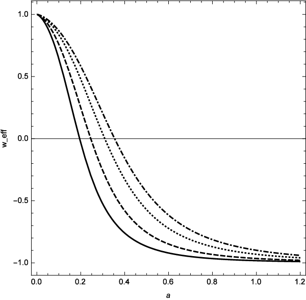
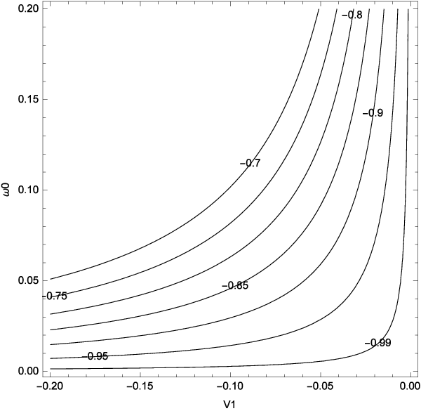
This explicitly Hubble function is used as a toy model to study the late-time acceleration of the universe. In Fig. 1, the qualitative evolution of the equation of state parameter for the solution (100) is presented for various values of the free parameters.

Refer to caption — Figure 1: Qualitative evolution of the effective equation of state parameter $w_{eff}$ for the Hubble function (100). Left fig. is the evolution with respect the scale factor for $a_{0}=1$ , $\omega_{0}=0.1$ and $V_{1}=-\frac{1}{2}10^{-3}\,\$ (solid line), $V_{1}=-10^{-2}$ (dash-dash line), $V_{1}=-2~10^{-2}$ (dot-dot line) and $V_{1}=-3$ $10^{-2}$ (dash-dot line). Right figure is the contour plot of $w_{eff}$ with respect to the free parameters $V_{1}$ and $\omega_{0}$ at the scale factor $a=1$ .

We continue our analysis with the analysis of the critical points for the field equations.

V The evolution of the flat FLRW spacetime on a phase space

From equation (24) one immediately sees that the Hubble function $H\left(t\right)$ can cross the value $H\left(t\right)=0$ , from negative to positive values, or vice-versa, since $\rho_{\phi}$ can be negative due the friction term $3H\dot{\phi}$ . Additionally, the effective potential $V(\phi)$ is not necessarily non-negative.

We introduce the new variables [90]:

x=\frac{\dot{\phi}}{\sqrt{(H^{2}+1)}},\quad y=\frac{V(\phi)}{6(H^{2}+1)},\quad z=\frac{H}{\sqrt{H^{2}+1}},

(101)

which are related through the relation

\Omega_{m}z^{2}=z(z-x)-y.

(102)

where $\Omega_{m}\equiv\frac{\rho_{m}}{3H^{2}}$ is not necessarily bounded, since $\rho_{\phi}$ and the effective potential $V(\phi)$ is not necessarily non-negative. Although, the interval $\Omega_{m}\in[0,1]$ corresponds to physically reasonable matter. We have assumed $w_{m}\in[-1,1]$ .
The evolution equations (24)-(27), are written in its autonomous form:


	$\displaystyle x^{\prime}=-3w_{m}(z(x-z)+y)-y(\lambda(xz-2)+3)+3z^{2}(xz-1),$	(103a)
	$\displaystyle y^{\prime}=y\left[6z^{3}-\lambda(x+2yz)\right],$	(103b)
	$\displaystyle z^{\prime}=\left(z^{2}-1\right)\left(3z^{2}-\lambda y\right),$	(103c)
	$\displaystyle\lambda^{\prime}=-h(\lambda)x.$	(103d)
where the prime means derivative with respect to a new time variable defined by

f^{\prime}\equiv\frac{df}{d\tau}=\frac{\dot{f}}{\sqrt{H^{2}+1}},

and $\lambda=-\frac{V_{,\phi}}{V}~,~h\left(\lambda\right)=\lambda^{2}\left(\frac{V_{,\phi\phi}}{\left(V_{,\phi}\right)^{2}}-1\right).$

For the choice $z=+1$ are recovered the equations investigated in [45]. From (103b) it follows that the sign of $y$ (i.e., the sign of $V(\phi)$ ) is invariant for the flow. Furthermore, by definition, $z$ has the same sign with $H$ , and from (103c) we have that $z^{\prime}|_{z=0}=\lambda y$ , which has not a definite sign. Observe that $z=\pm 1$ defines two invariant sets. Additionally, $z>0$ corresponds to expanding universe, whereas $z<0$ corresponds to contracting universes. Since the sign of $z$ is in general not invariant for the flow, the region of the phase space $z=0$ can be crossed which implies the existence of a transition from contracting, to expanding universes and viceversa. Furthermore, the system (103a)-(103c) is form invariant under the discrete symmetry $(x,z,\tau)\rightarrow(-x,-z,-\tau)$ . So that, the fixed points related by this symmetry have the opposite dynamical behavior. This implies that we can investigate just the dynamics in the region $x\geq 0,z\geq 0$ . However, we prefer to investigate the full region of the phase space, although, in the numerical examples we present the phase portraits for $z>0$ which corresponds to the region of cosmological interest since this leads to a phase of late accelerated expansion.
Finally, to extract some cosmological implications of the model at hand, we use the observables

\Omega_{\phi}=\frac{\rho_{\phi}}{3H^{2}},\quad q=-1-\frac{\dot{H}}{H^{2}},

(104)

which satisfy

\Omega_{\phi}=\frac{xz+y}{z^{2}},\quad q=2-\frac{\lambda y}{z^{2}},

(105)

are well-defined for $z\neq 0$ .

V.1 Exponential potential

Let us consider the model in which $\lambda^{\prime}$ is identically zero, that is $h(\lambda)=0$ , so that, we obtain the effective potential $V=V_{0}e^{-\lambda\phi}$ . We study the 3D dynamical system (103a), (103b), (103c), for $\lambda$ constant. In the following we consider $w_{m}\in\left[-1,1\right]$ . This case contains the potential $V_{D}$ given by (70) (see subsubsection IV.1.2) as the particular case $\lambda=3$ .

V.1.1 Description of the fixed points at the finite region of the phase space.

The (lines of) fixed points of the 3D dynamical system (103a), (103b), (103c), for $\lambda$ constant are the following:

1.

The line $A:(x,y,z)=\left(x_{c},0,0\right)$ , that contains the origin of coordinates. We cannot evaluate directly the expressions (105) at these points. The eigenvalues of the linearization of (103a), (103b), (103c) around the fixed point are $0,0,-\lambda x_{c}$ . Thus, it is nonhyperbolic.
2.

The point $B:(x,y,z)=\left(0,0,0\right)$ . We cannot evaluate directly the expressions (105) at this point. The eigenvalues of the linearization of (103a), (103b), (103c) around the fixed point are $0,0,0$ . Thus, it is nonhyperbolic.
3.

The line of fixed points $C(z_{c}):(x,y,z)=\left(0,z_{c}^{2},z_{c}\right)$ , $z_{c}\in[-1,1]$ , exists for $\lambda=3$ . Evaluating the expressions (105) we find $\Omega_{\phi}=1,q=-1.$ Thus, this represents a line of de-Sitter solutions. The eigenvalues of the linearization of (103a), (103b), (103c) around the line of fixed points are $0,-3z_{c},-3(w_{m}+1)z_{c}$ . Thus, it is nonhyperbolic.
1. (a)
  
  The stable manifold of $C(z_{c})$ is 2D for $0<z_{c}\leq 1,w_{m}>-1$ .
2. (b)
  
  The unstable manifold of $C(z_{c})$ is 2D for $-1\leq z_{c}<0,w_{m}>-1$ .
4.

$C(z_{c})$ contains the special point $D^{\pm}:(x,y,z)=\left(0,1,\epsilon\right),\epsilon=\pm 1$ . Evaluating the expressions (105) we find $\Omega_{\phi}=1,q=-1.$ Thus, this represents the endpoints of the previous line of de-Sitter solutions. The eigenvalues of the linearization of (103a), (103b), (103c) around the fixed point are $0,-3\epsilon,-3(w_{m}+1)\epsilon$ . Thus, it is nonhyperbolic.
1. (a)
  
  The stable manifold of $D^{+}$ is 2D for $w_{m}>-1$ .
2. (b)
  
  The unstable manifold if $D^{-}$ is 2D for $w_{m}>-1$ .
5.

The points $E^{\pm}:(x,y,z)=\left(\epsilon,0,\epsilon\right),\epsilon=\pm 1$ . Evaluating the expressions (105) we find $\Omega_{\phi}=1,q=2.$ So, they represents stiff solutions. The eigenvalues of the linearization of (103a), (103b), (103c) around the fixed point are $6\epsilon,3\epsilon(1-w_{m}),\epsilon\left[6-\lambda\right]$ .
1. (a)
  
  The points are nonhyperbolic for $w_{m}=1$ or $\lambda=6$ .
2. (b)
  
  The fixed point $E^{+}$ (respectively, $E^{-}$ ) is a source (respectively, a sink), for $w_{m}<1,\lambda<6$ .
3. (c)
  
  They are saddle otherwise.
6.

The points $F^{\pm}:(x,y,z)=\left(\epsilon\frac{3[w_{m}+1]}{{\lambda}},-\frac{3[w_{m}-1]}{2{\lambda}},\epsilon\right),\epsilon=\pm 1$ . Evaluating the expressions (105) we find $\Omega_{\phi}=\frac{3(w_{m}+3)}{2\lambda},q=\frac{1}{2}(3w_{m}+1)$ . So, they represent perfect fluid scaling solutions. The eigenvalues of the linearization of (103a), (103b), (103c) around the fixed point are $3(w_{m}+1)\epsilon,\frac{1}{4}\epsilon\left(3w_{m}-3-\sqrt{3}\sqrt{(1-w_{m})(-16\lambda+21w_{m}+75)}\right)$ ,
$\frac{1}{4}\epsilon\left(3w_{m}-3+\sqrt{3}\sqrt{(1-w_{m})(-16\lambda+21w_{m}+75)}\right)$ .
1. (a)
  
  The points are nonhyperbolic for either $w_{m}=-1$ , or $\lambda=\frac{3(w_{m}+3)}{2}$ , or $w_{m}=1$ .
2. (b)
  
  they are saddle otherwise.
7.

The points $G^{\pm}:(x,y,z)=\left(\epsilon\left[2-\frac{6}{{\lambda}}\right],\frac{6}{{\lambda}}-1,\epsilon\right),\epsilon=\pm 1$ . Evaluating the expressions (105) we find $\Omega_{\phi}=1,q=\lambda-4$ . So, they represent accelerating solutions for $\lambda<4$ . The eigenvalues of the linearization of (103a), (103b), (103c) around the fixed point are $(\lambda-6)\epsilon,2(\lambda-3)\epsilon,\epsilon(2\lambda-3w_{m}-9)$ .
1. (a)
  
  The points are nonhyperbolic for either $\lambda=6$ or $\lambda=3$ or $\lambda=\frac{3(w_{m}+3)}{2}$ .
2. (b)
  
  The fixed point $G^{+}$ (respectively, $G^{-}$ ) is a sink (respectively, a source) for $w_{m}>-1,\lambda<3$ .
3. (c)
  
  The fixed point $G^{+}$ (respectively, $G^{-}$ ) is a source (respectively, a sink) for $w_{m}\leq 1,\lambda>6$ .
4. (d)
  
  They are saddle otherwise.
  
  Figure 2: Array of phase portraits for the restriction of the dynamical system (103) for the exponential potential (i.e., $\lambda$ is a constant and $h\equiv 0$ ) on the invariant set $z=+1$ for a pressureless perfect fluid ( $w_{m}=0$ ), a radiation fluid ( $w=\frac{1}{3}$ ), and a stiff fluid ( $w_{m}=1$ ) for $\lambda=-3$ and $\lambda=1$ . The dotted (blue) line denotes the invariant set $y=0$ , whereas the region enclosed by the dot-dashed (red) line corresponds to the physical portion of the phase space.

V.1.2 Description of the fixed points at infinity.

For the description of the points at infinity we introduce the variables

x=\frac{1}{\rho}\cos\psi,\quad y=\frac{1}{\rho}\sin\psi,

(106)

and the time reescaling $f^{\prime}\rightarrow\rho f^{\prime}$ . Defining the new variables

X=\frac{x}{\sqrt{1+x^{2}+y^{2}}},\quad Y=\frac{y}{\sqrt{1+x^{2}+y^{2}}},

(107)

we obtain that the (lines of) fixed points at infinity are:

1.

The 2-parametric set $H(\psi,z_{c}):\left(X,Y,z\right)=\left(\cos\psi,\sin\psi,z_{c}\right),\quad\psi\in[0,2\pi]$ , which exist for $\lambda=0$ . The eigenvalues are $0,0,0.$ The set is nonhyperbolic.
2.

The points $I^{\pm}:\left(X,Y,z\right)=\left(\frac{\sqrt{2}}{2}\epsilon,-\frac{\sqrt{2}}{2},\epsilon\right)$ , $\epsilon=\pm 1$ . The eigenvalues are $\sqrt{2}\lambda\epsilon,-\frac{\sqrt{2}\lambda\epsilon}{2},\frac{\sqrt{2}\lambda\epsilon}{2}$ . Thus, they are saddles.
3.

The points $J^{\pm}:\left(X,Y,z\right)=\left(-\frac{\sqrt{2}}{2}\epsilon,\frac{\sqrt{2}}{2},\epsilon\right)$ , $\epsilon=\pm 1$ . The eigenvalues are $-\sqrt{2}\lambda\epsilon,-\frac{\lambda\sqrt{2}\epsilon}{2},\frac{\lambda\sqrt{2}\epsilon}{2}$ . Thus, they are saddles.
4.

The lines ${}_{\pm}K(z_{c}):\left(X,Y,z\right)=\left(\pm 1,0,z_{c}\right)$ , where the left subscript denotes de sign of $x$ . The eigenvalues are $0,0,\mp\lambda.$ Thus, these lines are nonhyperbolic.
5.

The lines $L^{\pm}:\left(X,Y,z\right)=\left(0,1,\epsilon\right)$ , $\epsilon=\pm 1$ . The eigenvalues are $-2\lambda\epsilon,\lambda\epsilon,2\lambda\epsilon$ . Thus, they are saddles.
6.

The lines $M^{\pm}:\left(X,Y,z\right)=\left(0,-1,\epsilon\right)$ , $\epsilon=\pm 1$ . The eigenvalues are $-2\lambda\epsilon,-\lambda\epsilon,2\lambda\epsilon$ . Thus, they are saddles.

We finish this section with a discussion of some numerical examples. In the figure 2 it is presented an array of phase portraits for the restriction of the dynamical system (103) for the exponential potential (i.e., $\lambda$ is a constant and $h\equiv 0$ ) on the invariant set $z=+1$ for a pressureless perfect fluid ( $w_{m}=0$ ), a radiation fluid ( $w=\frac{1}{3}$ ), and a stiff fluid ( $w_{m}=1$ ) for $\lambda=-3$ and $\lambda=1$ . The dotted (blue) line denotes the invariant set $y=0$ , whereas the region enclosed by the dot-dashed (red) line corresponds to the physical portion of the phase space. Furthermore, in Figure 3 it is presented an array of phase portraits for the restriction of the dynamical system (103) for the exponential potential (i.e., $\lambda$ is a constant and $h\equiv 0$ ) on the invariant set $z=+1$ a pressureless perfect fluid ( $w_{m}=0$ ), radiation ( $w_{m}=\frac{1}{3}$ ), and a stiff fluid ( $w_{m}=1$ ) for the bifurcation parameters $\lambda=3,\lambda=6$ . The dotted (blue) line denotes the invariant set $y=0$ , whereas the region enclosed by the dot-dashed (red) line corresponds to the physical portion of the phase space. For $\lambda=3$ the points $D^{+}$ and $G^{+}$ coincides. For $\lambda=6,w_{m}=1$ the points $D^{+}$ , $F^{+}$ and $G^{+}$ coincides.

V.2 Beyond the Exponential Potential

We continue our analysis with the case of a non-exponential potential in which the dynamical system is 4D.

V.2.1 Description of the fixed points at the finite region of the phase space.

The (lines of) fixed points of the 4D system (103) with finite coordinates are:

1.

The line $A:(x,y,z,\lambda)=\left(x_{c},0,0,0\right)$ , $h(0)=0$ . We cannot evaluate directly the expressions (105) at these points. The eigenvalues of the linearization of (103) around the line of fixed point are $0,0,0,-x_{c}h^{\prime}(0)$ . Thus, it is nonhyperbolic.
2.

The line $B:(x,y,z,\lambda)=\left(0,0,0,\lambda_{c}\right)$ . We cannot evaluate directly the expressions (105) at these points. The eigenvalues of the linearization of (103) around the line of fixed points are $0,0,0,0$ . Thus, it is nonhyperbolic.
3.

The line of fixed points $C(z_{c}):(x,y,z,\lambda)=\left(0,z_{c}^{2},z_{c},3\right)$ , $z_{c}\in[-1,1]$ . Evaluating the expressions (105) we find $\Omega_{\phi}=1,q=-1.$ Thus, this represents a line of de-Sitter solutions. The eigenvalues of the linearization of (103) around the line of fixed points are $0,-3(w_{m}+1)z_{c},-\frac{1}{2}\left(3+\sqrt{9-8h(3)}\right)z_{c},-\frac{1}{2}\left(3-\sqrt{9-8h(3)}\right)z_{c}$ .
1. (a)
  
  The stable manifold of $C(z_{c})$ is 3D for $0<z_{c}\leq 1,w_{m}>-1,h(3)>0$ .
2. (b)
  
  The unstable manifold of $C(z_{c})$ is 3D for $-1\leq z_{c}<1,w_{m}>-1,h(3)>0$ .
4.

$C(z_{c})$ contains the special point $D^{\pm}:(x,y,z,\lambda)=\left(0,1,\epsilon,3\right)$ , $\epsilon=\pm 1$ . Evaluating the expressions (105) we find $\Omega_{\phi}=1,q=-1,$ such that they are de Sitter solutions. The eigenvalues of the linearization of (103) around the fixed points are
$0,-3(w_{m}+1)\epsilon,-\frac{1}{2}\left(3+\sqrt{9-8h(3)}\right)\epsilon,-\frac{1}{2}\left(3-\sqrt{9-8h(3)}\right)\epsilon$ .
1. (a)
  
  The stable manifold of $D^{+}$ is 3D for $w_{m}>-1,h(3)>0$ .
2. (b)
  
  The unstable manifold of $D^{-}$ is 3D for $w_{m}>-1,h(3)>0$ .
5.

The points $E^{\pm}(\hat{\lambda}):(x,y,z,\lambda)=\left(\epsilon,0,\epsilon,\hat{\lambda}\right)$ , $\epsilon=\pm 1$ , and the values $\hat{\lambda}$ satisfy $h(\hat{\lambda})=0$ . Evaluating the expressions (105) we find $\Omega_{\phi}=1,q=2.$ So, they represents stiff solutions. The eigenvalues of the linearization of (103) around the fixed points are $6\epsilon,3(1-w_{m})\epsilon,\left(6-\hat{\lambda}\right)\epsilon,-\epsilon h^{\prime}(\hat{\lambda})$ .
1. (a)
  
  They are nonhyperbolic for $w_{m}=1$ , or $\hat{\lambda}=6$ , or $h^{\prime}(\hat{\lambda})=0$ .
2. (b)
  
  The fixed points $E^{+}(\hat{\lambda})$ (respectively, $E^{-}(\hat{\lambda})$ ) are sources (respectively, sinks), for $w_{m}<1,\hat{\lambda}<6,h^{\prime}(\hat{\lambda})<0$ .
3. (c)
  
  They are saddle otherwise.
6.

The points $F^{\pm}(\hat{\lambda}):(x,y,z,\lambda)=\left(\epsilon\frac{3[w_{m}+1]}{\hat{\lambda}},-\frac{3[w_{m}-1]}{2\hat{\lambda}},\epsilon,\hat{\lambda}\right)$ , $\epsilon=\pm 1$ , and the values $\hat{\lambda}\neq 0$ satisfy $h(\hat{\lambda})=0$ . Evaluating the expressions (105) we find $\Omega_{\phi}=\frac{3(w_{m}+3)}{2\hat{\lambda}},q=\frac{1}{2}(3w_{m}+1)$ . So, they represent perfect fluid scaling solutions. The eigenvalues of the linearization of (103) around the fixed points are $3(w_{m}+1)\epsilon$ ,
$-\frac{1}{4}\epsilon\left(3-3w_{m}-\sqrt{3}\sqrt{(1-w_{m})\left(-16\hat{\lambda}+21w_{m}+75\right)}\right)$ ,
$-\frac{1}{4}\epsilon\left(3-3w_{m}+\sqrt{3}\sqrt{(1-w_{m})\left(-16\hat{\lambda}+21w_{m}+75\right)}\right),$ $-\frac{3(w_{m}+1)\epsilon h^{\prime}(\hat{\lambda})}{\hat{\lambda}}$ .
1. (a)
  
  The points are nonhyperbolic for either $w_{m}=-1$ , or $\hat{\lambda}=\frac{3(w_{m}+3)}{2}$ , or $w_{m}=1$ , or $h^{\prime}(\hat{\lambda})=0$
2. (b)
  
  They are saddle otherwise.
7.

The points $G^{\pm}(\hat{\lambda}):(x,y,z,\lambda)=\left(\epsilon\left[2-\frac{6}{\hat{\lambda}}\right],\frac{6}{\hat{\lambda}}-1,\epsilon,\hat{\lambda}\right)$ , $\epsilon=\pm 1$ , and the values $\hat{\lambda}\neq 0$ satisfy $h(\hat{\lambda})=0$ . Evaluating the expressions (105) we find $\Omega_{\phi}=1,q=\hat{\lambda}-4$ . So, they represent accelerating solutions for $\hat{\lambda}<4$ . The eigenvalues of the linearization of (103) around the fixed points are $\left(\hat{\lambda}-6\right)\epsilon,2\left(\hat{\lambda}-3\right)\epsilon,\epsilon\left(2\hat{\lambda}-3w_{m}-9\right),-\frac{2\left(\hat{\lambda}-3\right)\epsilon h^{\prime}(\hat{\lambda})}{\hat{\lambda}}$ .
1. (a)
  
  The points are nonhyperbolic for either $\hat{\lambda}=6$ or $\hat{\lambda}=3$ or $\hat{\lambda}=\frac{3(w_{m}+3)}{2}$ or $h^{\prime}(\hat{\lambda})=0$ .
2. (b)
  
  The fixed point is $F^{+}$ (respectively, $F^{-}$ ) is a sink (respectively, a source) for
  1. i.
    
    $w_{m}>-1,\hat{\lambda}<0,h^{\prime}(\hat{\lambda})>0$ or
  2. ii.
    
    $w_{m}>-1,0<\hat{\lambda}<3,h^{\prime}(\hat{\lambda})<0$
3. (c)
  
  $F^{+}$ (respectively, $F^{-}$ ) is a source (respectively, a sink) for
  1. i.
    
    $w_{m}\leq 1,\hat{\lambda}>6,h^{\prime}(\hat{\lambda})<0$
4. (d)
  
  they are saddle otherwise.

V.2.2 Description of the fixed points at infinity.

For the description of the points when $x^{2}+y^{2}\rightarrow\infty$ we introduce the variables

x=\frac{1}{\rho}\cos\psi,\quad y=\frac{1}{\rho}\sin\psi,

and the time rescaling $f^{\prime}\rightarrow\rho f^{\prime}$ .

The (lines of) fixed points at infinity are:

1.

The 2-parametric set $H(\psi,z_{c}):\left(X,Y,z,\lambda\right)=\left(\cos\psi,\sin\psi,z_{c},0\right),\quad\psi\in[0,2\pi]$ , which exist for functions $h$ satisfying , $h(0)=0$ . The eigenvalues are $0,0,0,-h^{\prime}(0)\cos\psi$ .
2.

The points $I^{\pm}(\hat{\lambda}):\left(X,Y,z,\lambda\right)=\left(\frac{\sqrt{2}}{2}\epsilon,-\frac{\sqrt{2}}{2},\epsilon,\hat{\lambda}\right)$ , $\epsilon=\pm 1$ , and the values $\hat{\lambda}$ satisfy $h(\hat{\lambda})=0$ . The eigenvalues are $-\frac{\hat{\lambda}\epsilon}{\sqrt{2}},\frac{\hat{\lambda}\epsilon}{\sqrt{2}},\sqrt{2}\hat{\lambda}\epsilon,-\frac{\epsilon h^{\prime}\left(\hat{\lambda}\right)}{\sqrt{2}}$ . Thus they are saddles.
3.

The points $J^{\pm}(\hat{\lambda}):\left(X,Y,z,\lambda\right)=\left(-\frac{\sqrt{2}}{2}\epsilon,\frac{\sqrt{2}}{2},\epsilon,\hat{\lambda}\right)$ , $\epsilon=\pm 1$ , and the values $\hat{\lambda}$ satisfy $h(\hat{\lambda})=0$ . The eigenvalues are $-\frac{\hat{\lambda}\epsilon}{\sqrt{2}},\frac{\hat{\lambda}\epsilon}{\sqrt{2}},-\sqrt{2}\hat{\lambda}\epsilon,\frac{\epsilon h^{\prime}\left(\hat{\lambda}\right)}{\sqrt{2}}$ . Thus they are saddles.
4.

The lines ${}_{\pm}K(z_{c},\hat{\lambda}):\left(X,Y,z,\lambda\right)=\left(\epsilon,0,z_{c},\hat{\lambda}\right)$ , where the left subscript denotes de sign of $x$ , and the values $\hat{\lambda}$ satisfy $h(\hat{\lambda})=0$ . The eigenvalues are $0,0,\mp\hat{\lambda}\epsilon,\mp\epsilon h^{\prime}(\hat{\lambda})$ . Thus, these lines are nonhyperbolic.
5.

The lines $L^{\pm}(\lambda_{c}):\left(X,Y,z,\lambda\right)=\left(0,1,\epsilon,\lambda_{c}\right)$ , $\epsilon=\pm 1$ . These lines of fixed points exists independently of the functional form of $h$ . The eigenvalues are $-2\lambda\epsilon,\lambda\epsilon,2\lambda\epsilon,0$ . They are normally hyperbolic and behaves like saddles.
6.

The lines $M^{\pm}(\lambda_{c}):\left(X,Y,z,\lambda\right)=\left(0,-1,\epsilon,\lambda_{c}\right)$ , $\epsilon=\pm 1$ . These lines of fixed points exists independently of the functional form of $h$ . The eigenvalues are $-2\lambda\epsilon,-\lambda\epsilon,2\lambda\epsilon,0$ . They are normally hyperbolic and behaves like saddles.

V.2.3 Some specific potentials

In this section we discuss some examples.

Example 1: For the potential $V(\phi)=V_{0}e^{-\sigma\phi}+V_{1},\sigma\neq 0$ and $h\equiv-\lambda(\lambda-\sigma)$ . Observe that the system is form invariant under the discrete symmetry $(x,z,\tau)\rightarrow(-x,-z,-\tau)$ . So that, the fixed points related by this symmetry have the opposite dynamical behavior. The coordinates $(x,y,z,\lambda)$ of the fixed points and eigenvalues of Eqs. (103) with $h\equiv-\lambda(\lambda-\sigma)$ in the finite portion phase space with $x\geq 0,z\geq 0$ are the following:

1.

$A:(x,0,0,0)$ with eigenvalues $0,0,0,-x\sigma$ . They are nonhyperbolic.
2.

$A(\sigma):(x,0,0,\sigma)$ with eigenvalues $0,0,-x\sigma,x$ . They are nonhyperbolic (behaves as saddle since two eigenvalues has opposite signs).
3.

$B:(0,0,0,\lambda)$ with eigenvalues $0,0,0,0$ . Thus, they are nonhyperbolic.
4.

$B(\sigma):(0,0,0,\sigma)$ with eigenvalues $0,0,0,0$ . It is nonhyperbolic.
5.

$C(z):\left(0,z^{2},z,3\right)$ with eigenvalues $0,-3(w_{m}+1)z,-\frac{1}{2}z\left(\sqrt{81-24\sigma}+3\right)$ ,
$\frac{1}{2}z\left(\sqrt{81-24\sigma}-3\right)$ .
1. (a)
  
  The stable manifold of $C(z)$ is 3D for $0<z<1,w_{m}>-1,\sigma>3$ .
2. (b)
  
  The unstable manifold of $C(z)$ is 3D for $-1<z<0,w_{m}>-1,\sigma>3$ .
This line contains the points $D^{\pm}$ . Due the relevance of this lines in the cosmological setting (since they corresponds to de Sitter solutions), we proceed forward to analyze their stability using the Center Manifold Theory.
6.

$E^{+}(0):(1,0,1,0)$ with eigenvalues $6,6,3-3w_{m},-\sigma$ . Thus, it is
1. (a)
  
  Nonhyperbolic for $w_{m}=1$ .
2. (b)
  
  Source for $w_{m}<1,\sigma<0$ .
3. (c)
  
  Saddle otherwise.
7.

$E^{+}(\sigma):(1,0,1,\sigma)$ with eigenvalues $\{6,3-3w_{m},6-\sigma,\sigma\}$ . Thus, it is
1. (a)
  
  Nonhyperbolic for $w_{m}=1$ , or $\sigma=6$ .
2. (b)
  
  Source for $w_{m}<1,0<\sigma<6$ .
3. (c)
  
  Saddle otherwise.
8.

$F^{+}(\sigma):\left(\frac{3(w_{m}+1)}{\sigma},-\frac{3(w_{m}-1)}{2\sigma},1,\sigma\right)$ with eigenvalues $3(w_{m}+1),3(w_{m}+1)$ ,
$\frac{1}{4}\left(3w_{m}-3-\sqrt{3(1-w_{m})(21w_{m}-16\sigma+75)}\right)$ ,
$\frac{1}{4}\left(3w_{m}-3+\sqrt{3(1-w_{m})(21w_{m}-16\sigma+75)}\right)$ .
1. (a)
  
  $F^{+}(\sigma)$ is nonhyperbolic for either $w_{m}=-1$ , or $\sigma=\frac{3(w_{m}+3)}{2}$ , or $w_{m}=1$ .
2. (b)
  
  It is saddle otherwise.
9.

$G^{+}(\sigma):\left(\frac{2(\sigma-3)}{\sigma},\frac{6-\sigma}{\sigma},1,\sigma\right)$ with eigenvalues $\sigma-6,2(\sigma-3),2(\sigma-3),-3w_{m}+2\sigma-9$ . Thus, it is
1. (a)
  
  Nonhyperbolic for $\sigma\in\left(3,6,\frac{3}{2}(3+w_{m})\right)$ .
2. (b)
  
  Source for $w_{m}\leq 1,\sigma>6$ , or $w_{m}>1,\sigma>\frac{3(w_{m}+3)}{2}$ .
3. (c)
  
  Sink for $w_{m}\leq-1,\sigma<\frac{3(w_{m}+3)}{2}$ , or $w_{m}>-1,\sigma<3$ .
4. (d)
  
  Saddle otherwise.

Example 2: Power-law potential $V\left(\phi\right)=\frac{(\mu\phi)^{k}}{k}$ with $h\equiv-\frac{\lambda^{2}}{k}.$ This case contains the potential $V_{A}$ defined by (63) and discussed in subsubsection IV.1.1, for the particular choice $k=1,V_{1}=\mu,V_{0}=0$ . As before, the system is form invariant under the discrete symmetry $(x,z,\tau)\rightarrow(-x,-z,-\tau)$ , so that, we can investigate just the dynamics in the region $x\geq 0,z\geq 0$ . The coordinates $(x,y,z,\lambda)$ of the fixed points and the eigenvalues for Eqs. (103) with $h\equiv-\frac{\lambda^{2}}{k}$ in the finite portion phase space with $x\geq 0,z\geq 0$ are the following:

1.

$A:(x,0,0,0)$ with eigenvalues $0,0,0,0$ ; thus, it is nonhyperbolic.
2.

$B:(0,0,0,\lambda)$ with eigenvalues $0,0,0,0$ ; thus, it is nonhyperbolic.
3.

$C(z):\left(0,z^{2},z,3\right)$ with eigenvalues
$0,-3(w_{m}+1)z,-\frac{3\left(k+\sqrt{k(k+8)}\right)z}{2k},-\frac{3\left(k-\sqrt{k(k+8)}\right)z}{2k}$ .
1. (a)
  
  The stable manifold is 3D for $z>0,-1<w_{m}\leq 1,k\leq-8$ .
2. (b)
  
  The unstable manifold is 3D for $z<0,-1<w_{m}\leq 1,k\leq-8$ .
This line contains the points $D^{\pm}$ .
4.

$E^{+}(0):(1,0,1,0)$ with $\{6,6,0,3-3w_{m}\}$ ; thus, it is nonhyperbolic.

Since all the fixed points are nonhyperbolic we rely on numerical inspection. However, for the line of de Sitter solutions $C(z)$ we implement the Center Manifold computation.

Example 3: Hyperbolic Potential $V(\phi)=V_{0}(\cosh(\xi\phi)-1),\xi\neq 0$ , and $h\equiv-\frac{1}{2}\left(\lambda^{2}-\xi^{2}\right)$ . As before, the system is form invariant under the discrete symmetry $(x,z,\tau)\rightarrow(-x,-z,-\tau)$ , so that, we can investigate just the dynamics in the region $x\geq 0,z\geq 0$ . The coordinates $(x,y,z,\lambda)$ of the fixed points and eigenvalues for Eqs. (103) with $h\equiv-\frac{1}{2}\left(\lambda^{2}-\xi^{2}\right)$ in the finite portion phase space with $x\geq 0,z\geq 0$ are given by:

1.

$A(-\xi):(x,0,0,-\xi)$ with eigenvalues $0,0,-x\xi,x\xi$ . They are nonhyperbolic (behaves a saddles).
2.

$A(\xi):(x,0,0,\xi)$ with eigenvalues $0,0,-x\xi,x\xi$ . They are nonhyperbolic (behaves a saddles).
3.

$B:(0,0,0,\lambda)$ with eigenvalues $0,0,0,0$ . They are nonhyperbolic.
4.

$B(-\xi):(0,0,0,-\xi)$ with eigenvalues $0,0,0,0$ . It is nonhyperbolic.
5.

$B(\xi):(0,0,0,\xi)$ with eigenvalues $0,0,0,0$ . It is nonhyperbolic.
6.

$C(z):\left(0,z^{2},z,3\right)$ with eigenvalues
$0,-3(w_{m}+1)z,\frac{z}{2}\left(-3-\sqrt{45-4\xi^{2}}\right),\frac{z}{2}\left(-3+\sqrt{45-4\xi^{2}}\right)$ .
1. (a)
  
  The stable manifold is 3D for $z>0,-1<w_{m}\leq 1,-\frac{3\sqrt{5}}{2}\leq\xi<-3$ or $z>0,-1<w_{m}\leq 1,3<\xi\leq\frac{3\sqrt{5}}{2}$ .
2. (b)
  
  The unstable manifold is 3D for $z<0,-1<w_{m}\leq 1,-\frac{3\sqrt{5}}{2}\leq\xi<-3$ or $z<0,-1<w_{m}\leq 1,3<\xi\leq\frac{3\sqrt{5}}{2}$ .
This line contains the points $D^{\pm}$ .
7.

$E^{+}(-\xi):(1,0,1,-\xi)$ with eigenvalues $6,3-3w_{m},-\xi,\xi+6$ . It is
1. (a)
  
  Nonhyperbolic for $w_{m}=1$ , or $\xi=-6$ .
2. (b)
  
  source for $-6<\xi<0,w_{m}<1$ .
3. (c)
  
  saddle otherwise.
8.

$E^{+}(\xi):(1,0,1,\xi)$ with eigenvalues $6,3-3w_{m},6-\xi,\xi$ . It is
1. (a)
  
  Nonhyperbolic for $w_{m}=1$ , or $\xi=6$ .
2. (b)
  
  source for $0<\xi<6,w_{m}<1$ .
3. (c)
  
  saddle otherwise.
9.

$F^{+}(-\xi):\left(-\frac{3(w_{m}+1)}{\xi},\frac{3(w_{m}-1)}{2\xi},1,-\xi\right)$ with eigenvalues
$3(w_{m}+1),3(w_{m}+1),\frac{3(w_{m}-1)-\sqrt{3}\sqrt{-(w_{m}-1)(21w_{m}+16\xi+75)}}{4},\frac{3(w_{m}-1)+\sqrt{3}\sqrt{-(w_{m}-1)(21w_{m}+16\xi+75)}}{4}$ .
1. (a)
  
  $F^{+}(-\xi)$ is nonhyperbolic for either $w_{m}=-1$ , or $\xi=-\frac{3(w_{m}+3)}{2}$ , or $w_{m}=1$ .
2. (b)
  
  It is saddle otherwise.
10.

$F^{+}(\xi):\left(\frac{3(w_{m}+1)}{\xi},-\frac{3(w_{m}-1)}{2\xi},1,\xi\right)$ with eigenvalues
$3(w_{m}+1),3(w_{m}+1),\frac{3(w_{m}-1)-\sqrt{3}\sqrt{-(w_{m}-1)(21w_{m}-16\xi+75)}}{4},\frac{3(w_{m}-1)+\sqrt{3}\sqrt{-(w_{m}-1)(21w_{m}-16\xi+75)}}{4}$ .
1. (a)
  
  $F^{+}(\xi)$ is nonhyperbolic for either $w_{m}=-1$ , or $\xi=\frac{3(w_{m}+3)}{2}$ , or $w_{m}=1$ .
2. (b)
  
  It is saddle otherwise.
11.

$G^{+}(-\xi):\left(\frac{2(\xi+3)}{\xi},\frac{-\xi-6}{\xi},1,-\xi\right)$ with eigenvalues
$-2(\xi+3),-2(\xi+3),-3w_{m}-2\xi-9,-\xi-6$ . It is
1. (a)
  
  Nonhyperbolic for $\xi\in\left(-3,-6,-\frac{3}{2}(3+w_{m})\right)$ .
2. (b)
  
  Source for $w_{m}\leq 1,\xi<-6$ or $w_{m}>1,\xi<-\frac{3(w_{m}+3)}{2}$ .
3. (c)
  
  Sink for $w_{m}\leq-1,\xi>-\frac{3(w_{m}+3)}{2}$ or $w_{m}>-1,\xi>-3$ .
4. (d)
  
  Saddle otherwise.
12.

$G^{+}(\xi):\left(\frac{2(\xi-3)}{\xi},\frac{6-\xi}{\xi},1,\xi\right)$ with eigenvalues $\xi-6,2(\xi-3),2(\xi-3),-3w_{m}+2\xi-9$ . It is
1. (a)
  
  Nonhyperbolic for $\xi\in\left(3,6,\frac{3}{2}(3+w_{m})\right)$ .
2. (b)
  
  Source for $w_{m}\leq 1,\xi>6$ or $w_{m}>1,\xi>\frac{3(w_{m}+3)}{2}$ .
3. (c)
  
  Sink for $w_{m}\leq-1,\xi<\frac{3(w_{m}+3)}{2}$ or $w_{m}>-1,\xi<3$ .
4. (d)
  
  Saddle otherwise.

V.3 Critical points for potentials supported by Cartan symmetries

Finally, we discuss some models that were introduced by the Cartan symmetries in Section IV.
Example 4: For the potential $V_{B}\left(\phi\right)$ we calculate $h_{B}\equiv-\left(\lambda-3(w_{m}+1)\right)(\lambda-6w_{m})~$ . Due to the existence of the discrete symmetry $(x,z,\tau)\rightarrow(-x,-z,-\tau)$ , the fixed points related by this symmetry have the opposite dynamical behavior. The coordinates $(x,y,z,\lambda)$ of the fixed points and eigenvalues for Eqs. (103) with $h\equiv-(\lambda-6w_{m})\left(\lambda-3(w_{m}+1)\right)$ in the finite portion phase space with $x\geq 0,z\geq 0$ are the following.

1.

$A_{1}:(x,0,0,6w_{m})$ with eigenvalues $0,0,3(w_{m}-1)x,-6w_{m}x$ .
1. (a)
  
  The stable manifold of $A_{1}$ is 2D for $0<w_{m}<1,x>0$ .
2. (b)
  
  The unstable manifold of $A_{1}$ is 2D for $0<w_{m}<1,x<0$ .
2.

$A_{2}:(x,0,0,3(w_{m}+1))$ with eigenvalues $0,0,-3(w_{m}-1)x,-3(w_{m}+1)x$ . The nonzero eigenvalues has different signs for $-1<w_{m}<1,x\neq 0$ . Thus, it behaves as a saddle.
3.

$B:(0,0,0,\lambda)$ with eigenvalues $0,0,0,0$ . They are nonhyperbolic.
4.

$B_{1}:(0,0,0,6w_{m})$ with eigenvalues $0,0,0,0$ . It is nonhyperbolic.
5.

$B_{2}:(0,0,0,3(w_{m}+1))$ with eigenvalues $0,0,0,0$ . It is nonhyperbolic.
6.

$C(z):\left(0,z^{2},z,3\right)$ with eigenvalues $0,-6w_{m}z,-3(w_{m}+1)z,3(2w_{m}-1)z$ .
1. (a)
  
  Its stable manifold is 3D for $0<w_{m}<\frac{1}{2},z>0$ .
2. (b)
  
  Its unstable manifold is 3D for $0<w_{m}<\frac{1}{2},z<0$ .
This curve contains the points $D^{\pm}$ .
7.

$E^{+}_{1}:(1,0,1,6w_{m})$ with eigenvalues $6,3-3w_{m},6-6w_{m},3(w_{m}-1)$ .
1. (a)
  
  It is nonhyperbolic for $w_{m}=1$ .
2. (b)
  
  It is a saddle otherwise.
8.

$E^{+}_{2}:(1,0,1,3(w_{m}+1))$ with eigenvalues $6,3-3w_{m},3-3w_{m},3-3w_{m}$ .
1. (a)
  
  It is nonhyperbolic for $w_{m}=1$ .
2. (b)
  
  It is a source for $w_{m}<1$ .
9.

$F^{+}_{1}:\left(\frac{w_{m}+1}{2w_{m}},\frac{1-w_{m}}{4w_{m}},1,6w_{m}\right),w_{m}\neq 0$ , with eigenvalues $\frac{3\left(w_{m}^{2}-1\right)}{2w_{m}},3(w_{m}+1)$ ,
$3-3w_{m},\frac{9(w_{m}-1)}{2}$ .
1. (a)
  
  It is nonhyperbolic for $w_{m}\in\{-1,1\}$ .
2. (b)
  
  Saddle otherwise.
10.

$F^{+}_{2}:\left(1,\frac{1-w_{m}}{2(w_{m}+1)},1,3(w_{m}+1)\right),w_{m}\neq-1$ , with eigenvalues
$3-3w_{m},-\frac{3}{2}(w_{m}-1),3(w_{m}-1),3(w_{m}+1)$ .
1. (a)
  
  It is nonhyperbolic for $w_{m}=1$ .
2. (b)
  
  Saddle otherwise.
11.

$G^{+}_{1}:\left(\frac{2w_{m}-1}{w_{m}},\frac{1-w_{m}}{w_{m}},1,6w_{m}\right),w_{m}\neq 0$ , with eigenvalues $6w_{m}-9+\frac{3}{w_{m}}$ ,
$12w_{m}-6,6(w_{m}-1),9(w_{m}-1)$ .
1. (a)
  
  Nonhyperbolic for $w_{m}\in\left(\frac{1}{2},1\right)$
2. (b)
  
  It is a sink for $-1\leq w_{m}<0$ .
3. (c)
  
  It is a saddle otherwise.
12.

$G^{+}_{2}:\left(\frac{2w_{m}}{w_{m}+1},\frac{1-w_{m}}{w_{m}+1},1,3(w_{m}+1)\right),w_{m}\neq-1$ , with eigenvalues $-\frac{6(w_{m}-1)w_{m}}{w_{m}+1},6w_{m}$ ,
$3(w_{m}-1),3(w_{m}-1)$ .
1. (a)
  
  Nonhyperbolic for $w_{m}\in\left(0,1\right)$
2. (b)
  
  It is a sink for $-1<w_{m}<0$ .
3. (c)
  
  It is a saddle otherwise.

We have used subscripts to distinguish each particular member of a class, instead to specify $\hat{\lambda}$ , to avoid a cumbersome notation. The subscript $1$ means evaluation at $\hat{\lambda}=6w_{m}$ , whereas, the subscript $2$ means evaluation at $\hat{\lambda}=3(w_{m}+1)$ .

Example 5: For the potential $V_{C}\left(\phi\right)$ we calculate $h_{C}\equiv-\frac{1}{2}\left(\lambda-3(w_{m}+1)\right)\left(2\lambda-3(3+w_{m})\right)~$ . Due to the existence of the discrete symmetry $(x,z,\tau)\rightarrow(-x,-z,-\tau)$ , the fixed points related by this symmetry have the opposite dynamical behavior. The coordinates $(x,y,z,\lambda)$ of the fixed points and eigenvalues for Eqs. (103) with $h\equiv-\frac{1}{2}\left(\lambda-3(w_{m}+1)\right)\left(2\lambda-3(3+w_{m})\right)$ in the finite portion phase space with $x\geq 0,z\geq 0$ are the following.

1.

$A_{1}:\left(x,0,0,\frac{3(w_{m}+3)}{2}\right)$ with eigenvalues $0,0,-\frac{3}{2}(w_{m}-1)x,-\frac{3}{2}(w_{m}+3)x$ . They are nonhyperbolic (behaves as saddles for $x\neq 0$ ).
2.

$A_{2}:(x,0,0,3(w_{m}+1))$ with eigenvalues $0,0,\frac{3}{2}(w_{m}-1)x,-3(w_{m}+1)x$ . They are nonhyperbolic (behaves as saddles for $x\neq 0$ ).
3.

$B:(0,0,0,\lambda)$ with eigenvalues $0,0,0,0$ . They are nonhyperbolic.
4.

$B_{1}:\left(0,0,0,\frac{3(w_{m}+3)}{2}\right)$ with eigenvalues $0,0,0,0$ . It is nonhyperbolic.
5.

$B_{2}:(0,0,0,3(w_{m}+1))$ with eigenvalues $0,0,0,0$ . It is nonhyperbolic.
6.

$C(z):\left(0,z^{2},z,3\right)$ with eigenvalues $0,3w_{m}z,-3(w_{m}+1)z,-3(w_{m}+1)z$ .
1. (a)
  
  Its stable manifold is 3D for $-1<w_{m}<0,z>0$ .
2. (b)
  
  Its unstable manifold is 3D for $-1<w_{m}<0,z<0$ .
This curve contains the points $D^{\pm}$ .
7.

$E^{+}_{1}:\left(1,0,1,\frac{3(w_{m}+3)}{2}\right)$ with eigenvalues $6,-3(w_{m}-1),-\frac{3}{2}(w_{m}-1),-\frac{3}{2}(w_{m}-1)$ .
1. (a)
  
  It is nonhyperbolic for $w_{m}=1$ .
2. (b)
  
  It is a source for $w_{m}<1$ .
8.

$E^{+}_{2}:(1,0,1,3(w_{m}+1))$ with eigenvalues $6,-3(w_{m}-1),-3(w_{m}-1),\frac{3(w_{m}-1)}{2}$ .
1. (a)
  
  It is nonhyperbolic for $w_{m}=1$ .
2. (b)
  
  It is a saddle otherwise.
9.

$F^{+}_{1}:\left(\frac{2(w_{m}+1)}{w_{m}+3},\frac{1-w_{m}}{w_{m}+3},1,\frac{3(w_{m}+3)}{2}\right)$ with eigenvalues $0,\frac{3-3w_{m}^{2}}{w_{m}+3},3(w_{m}+1),\frac{3(w_{m}-1)}{2}$ . It is nonhyperbolic. The zero eigenvalue appears due to the bifurcation value $\hat{\lambda}$ , where $F^{+}_{1}$ and $G^{+}_{1}$ coincide. It behaves a saddle (at least two eigenvalues are of different sign).
10.

$F^{+}_{2}:\left(1,\frac{1-w_{m}}{2(w_{m}+1)},1,3(w_{m}+1)\right),w_{m}\neq-1$ , with eigenvalues
$-\frac{3}{2}(w_{m}-1),\frac{3(w_{m}-1)}{2},3(w_{m}-1),3(w_{m}+1)$ .
1. (a)
  
  It is nonhyperbolic for $w_{m}=1$ .
2. (b)
  
  It is a saddle otherwise.
11.

$G^{+}_{1}$ merges with $F^{+}_{1}$ . Thus, it behaves as saddle.
12.

$G^{+}_{2}:\left(\frac{2w_{m}}{w_{m}+1},\frac{1-w_{m}}{w_{m}+1},1,3(w_{m}+1)\right)$ with eigenvalues
$\frac{3(w_{m}-1)w_{m}}{w_{m}+1},6w_{m},3(w_{m}-1),3(w_{m}-1)$ .
1. (a)
  
  Nonhyperbolic for $w_{m}\in\left(0,1\right)$
2. (b)
  
  It is a saddle otherwise.

VI Toy model and Supernova data

Consider now the Hubble parameter

E(a)=\frac{H\left(a\right)}{H_{0}}=\Omega_{\Lambda 0}\left(1+\sqrt{1+\frac{\Omega_{s0}}{\Omega_{\Lambda 0}}a^{-3}}\right)+\Omega_{s0}a^{-3},

(108)

where if we compare it with (100) it follows that $\Omega_{\Lambda 0}=\left(12\left(a_{0}\right)^{3}\left(-V_{1}\right)H_{0}\right)^{-1}$ and $\Omega_{s0}=2\omega_{0}H_{0}^{-1}$ . It is clear that from that Hubble function, except from the cosmological constant term and the stiff fluid, there is also a term which provides a dark energy component. This is not the first time that this noncanonical scalar field provide dust terms in the cosmological solution. It has been observed before in [45, 46].

Moreover, from the constraint $H\left(a\rightarrow 1\right)=H_{0}$ , we find the algebraic relation between the two free parameters $\Omega_{\Lambda 0}$ and $\Omega_{s0}$ ,

\Omega_{\Lambda 0}=\frac{1-\Omega_{s0}}{2-\Omega_{s0}}.

(109)

which is used to reduce the free parameters of the model. It is interesting to mention that the current model contains the same number of free parameters with that of the concordance $\Lambda$ CDM model.

We continue by constraining the Hubble function (108) with some of the cosmological data. In particular we perform a joint likelihood analysis in order to constraint the one free parameter, $\Omega_{s0}$ , by using the SNIa data of the Union 2.1 collaboration [91].

The likelihood function is determined to be $\mathcal{L}\mathcal{=}e^{-\chi_{A}^{2}/2}~$ ; that is, $\chi^{2}=\chi_{SNIa}^{2}$ and the Likelihood function is maximized for the minimum parameter of $\chi^{2}$ . The Union 2.1 data set provides us with 580 SNIa distance modulus at observed redshift [91] with observed redshift in the range $z_{i}\in$ $\left[0.015,1.414\right]$ . The chi-square parameter for the diagonal covariant matrix is given by the expression

\chi_{SNIa}^{2}(\mathbf{\epsilon})=\sum\limits_{i=1}^{N_{SNIa}}\left(\frac{\mu_{obs}\left(z_{i}\right)-\mu_{th}\left(z_{i},\mathbf{\epsilon}\right)}{\sigma_{i}}\right)^{2}

(110)

where $\mathbf{\epsilon}\equiv\{H_{0},p^{1},p^{2},...\}$ denotes the statistical vector that contains the free parameters of the model, $N_{SNIa}=580$ , $z_{i}$ is the observed redshift, $\mu_{obs}$ is the observed distance modulus and $\mu_{th}$ is the theoretical distance modulus which is given by

\mu=m-M=5\log d_{L}+25=5\log D_{L}+\mu_{0},

(111)

where

d_{L}(\mathbf{\epsilon},z)=\frac{c}{H_{0}}D_{L}(p^{j},z)=\frac{c}{H_{0}}\int_{0}^{z}\frac{dx}{E(x,p^{j})}

(112)

and $\mu_{0}=42.384-5\log h$ with $h=H_{0}/100$ . Including the second equality of Eq.(111) into Eq.(110) we arrive at

\chi_{SNIa}^{2}(\mathbf{\epsilon})=A-2B\mu_{0}+\Gamma\mu_{0}^{2},

(113)

where

A(p^{j})=\sum\limits_{i=1}^{N_{SNIa}}\left(\frac{\mu_{obs}\left(z_{i}\right)-5\log D_{L}\left(z_{i},p^{j}\right)}{\sigma_{i}}\right)^{2}

(114)

B(p^{j})=\sum\limits_{i=1}^{N_{SNIa}}\frac{\mu_{obs}\left(z_{i}\right)-5\log D_{L}\left(z_{i},p^{j}\right)}{\sigma_{i}^{2}}

(115)

\Gamma=\sum\limits_{i=1}^{N_{SNIa}}\frac{1}{\sigma_{i}^{2}}\;.

(116)

Clearly, for $\mu_{0}=B/\Gamma$ , (113) has a minimum at

{\tilde{\chi}}_{SNIa}^{2}(p^{j})=A(p^{j})-\frac{\left(B(p^{j})\right)^{2}}{\Gamma}.

The latter implies that instead of using $\chi_{SNIa}^{2}(\mathbf{\epsilon})$ we now minimize ${\tilde{\chi}}_{SNIa}^{2}(p^{j})$ which is independent of $\mu_{0}$ and hence of the value of the Hubble constant. Therefore, for the current model we have only one free parameter, namely $p^{1}=\Omega_{s0}$ . The reader may find more details regarding the aforementioned statistical procedure in [92].

We compare the model (108) with that of the $\Lambda$ -cosmology whose Hubble function is

\frac{H_{\Lambda}\left(a\right)}{H_{0}}=\sqrt{\left(1-\Omega_{m0}\right)+\Omega_{m0}a^{-3}}.

(117)

In this case the free parameter of the model is $p^{1}=\Omega_{m0}$ .

From the SNIa data we found that $\left(\min\chi^{2}\right)=562.77$ while the best fit value is $\Omega_{s0}=0.0835_{-0.055}^{+0.065}.$ With the same data for the $\Lambda$ -cosmology we find that $\Omega_{m0}=0.29$ with $\left(\min\chi^{2}\right)^{\Lambda}=561.73$ .

The two models have the same number of degrees of freedom and the difference of the minimum $\chi^{2}$ is approximately one. Therefore according to the Akaike information criterion [93, 94] the two models fit the Supernova data with the same way.

Of course, model (108) has been used as a toy model in order to show that the model we proposed and the solutions which result provide parameters which allow it to fit the cosmological observations. Further extended analysis is required, which however is beyond the scope of the present study.

VII Evolution of the observables

Following the reference [108], we choose $t=0$ corresponding to the initial singularity, and denote $t_{0}$ as the age of the universe. The current value $H_{0}$ of the Hubble scalar is called the Hubble constant. For these quantities we have observable bounds. Now, we introduce the dimensionless parameters

\alpha=tH,\beta=\frac{\dot{\phi}}{H}.

(118)

The present value of $\alpha$ , denoted by $\alpha_{0}=t_{0}H_{0}$ is referred as the age parameter and it is a well-defined function in state space [108]. In an ever expanding model, where $a=a_{0}e^{N}$ , the numbers of e-foldings $N$ assume all real values, thus we can study the dynamical system


	$\displaystyle\frac{d{\Omega_{\phi}}}{dN}=(\Omega_{\phi}-1)(2q-3w_{m}-1),$	(119a)
	$\displaystyle\frac{d{\beta}}{dN}=(q(\beta-2)-3(w_{m}+1)\Omega_{\phi}+3w_{m}+4\beta+1),$	(119b)
	$\displaystyle\frac{d{\lambda}}{dN}=-\beta h(\lambda),$	(119c)
	$\displaystyle q=2+\lambda(\beta-\Omega_{\phi}),$	(119d)
and the decoupled equation

\frac{d{\alpha}}{dN}=1-(1+q)\alpha.

(120)

The latter algebraic-differential system is exactly the system (103a)-(103d) but in different variables.

Let us denote by $y$ the vector $\left(\Omega_{\phi},\beta,\lambda\right)$ . We have seen that $q$ is a function of the phase space as defined by (119d). Hence, at a fixed point $y^{\star}$ of the DE (119), $q$ is a constant, i.e., $q(y^{\star})$ , (the particular values of $q$ are summarized in the Appendix B). Given an initial point $\mathbf{y}_{0}$ - which represents our universe in the present time, let denoted by $\mathbf{y}=\Phi_{N}(\mathbf{y}_{0})$ the orbit through $\mathbf{y}_{0}$ with $\Phi_{0}(\mathbf{y}_{0})=\mathbf{y}_{0}$ , and by

\tilde{q}(N)=q(\Phi_{N}(\mathbf{y}_{0})),

(121)

the deceleration parameter along the orbit so that $\tilde{q}(0)=q(\mathbf{y}_{0})$ .

Then, are deduced the expressions [108]:


	$\displaystyle H(N)=H_{0}\exp\left[-\int_{0}^{N}\left\{1+\tilde{q}(\mu)\right\}d\mu\right],\;\text{for all}\;N\in\mathbb{R}.$	(122a)
	$\displaystyle t_{0}=\int_{-\infty}^{0}\frac{1}{H(N)}dN,$	(122b)
	$\displaystyle t_{0}H_{0}=\int_{-\infty}^{0}\exp\left[\int_{0}^{N}\left\{1+\tilde{q}(\mu)\right\}d\mu\right]dN$	(122c)
where $H_{0}$ is a freely specifiable. This arbitrariness implies that each non-singular orbit corresponds to a 1-parameter family of physical universes, which are conformally related by a constant rescaling of the metric. $t_{0}=t(0)$ , denotes the value of $t$ at $\mathbf{y}_{0}$ . The last formula implies that $\alpha_{0}=t_{0}H_{0}$ is uniquely determined by the specified initial point $\mathbf{y}_{0}$ on the phase space, such that $\alpha_{0}=t_{0}H_{0}$ is a well-defined function on state space. Furthermore, the constraints $0.87<\alpha(\mathbf{y}_{0})<1.68$ , $0.1\lesssim\Omega_{0}\lesssim 0.3$ [108], where $\Omega_{0}=1-\Omega_{\phi}(\mathbf{y}_{0})$ , will restrict the location of the present state of the universe, $\mathbf{y}_{0}$ , in state space.

Evaluating at the fixed points of (119), we have found the cosmological solutions:

		$\displaystyle(\Omega_{\phi},\alpha,\beta,\lambda)=\left(1,\frac{1}{3},1,\hat{\lambda}\right),H=\frac{1}{3t},q=2.$		(123)
		$\displaystyle F^{+}(\hat{\lambda}):\left(\frac{3\left(w_{m}+3\right)}{2\hat{\lambda}},\frac{2}{3\left(w_{m}+1\right)},\frac{3\left(w_{m}+1\right)}{\hat{\lambda}},\hat{\lambda}\right),H=\frac{2}{3\left(w_{m}+1\right)}t^{-1},q=\frac{1}{2}\left(3w_{m}+1\right).$		(124)
		$\displaystyle G^{+}(\hat{\lambda}):\left(1,\frac{1}{\hat{\lambda}-3},2-\frac{6}{\hat{\lambda}},\hat{\lambda}\right),H=\frac{1}{\hat{\lambda}-3}t^{-1},q=\hat{\lambda}-4.$		(125)

where we used the notation $\hat{\lambda}=h^{(-1)}(0)$ . Using the above normalization, the result is the “scaling away” of the effects of the overall expansion. However, in order to relate the analysis to observations, the equations that determine the evolution of $H$ , and clock time have to brought into play [108]. The equations (119) can be written as


	$\displaystyle\frac{d{\Omega_{\phi}}}{d\ln t}=\alpha(\Omega_{\phi}-1)(2q-3w_{m}-1),$	(126a)
	$\displaystyle\frac{d{\alpha}}{d\ln t}=-\alpha(\alpha+\alpha q-1),$	(126b)
	$\displaystyle\frac{d{\beta}}{d\ln t}=\alpha(q(\beta-2)-3(w_{m}+1)\Omega_{\phi}+3w_{m}+4\beta+1),$	(126c)
	$\displaystyle\frac{d{\lambda}}{d\ln t}=-\alpha\beta h(\lambda),$	(126d)
where

q=2+\lambda(\beta-\Omega_{\phi}).

(127)

Since we have assumed $0\leq t<\infty$ , then $-\infty<\ln t<+\infty$ is a good time parameter for the dynamical system. The coordinates $(\Omega_{\phi},\alpha,\beta,\lambda)$ of the fixed points of (119) can be generically written as follows:

1.

$\left(\Omega_{\phi},0,\frac{q-2}{\lambda}+\Omega_{\phi},\lambda\right)$ , eigenvalues $\left\{0,0,0,\frac{\lambda-3\lambda w_{m}\left(\Omega_{\phi}-1\right)+\lambda(q+1)\Omega_{\phi}+q(-2\lambda+q+2)-8}{\lambda}\right\}$ .
2.

$\left(1,0,\frac{q+\lambda-2}{\lambda},\lambda\right)$ , eigenvalues: $0,0,0,\frac{(q-2)(-\lambda+q+4)}{\lambda}$ .
3.

$\left(\Omega_{\phi},0,\frac{q-2}{\hat{\lambda}}+\Omega_{\phi},\hat{\lambda}\right)$ , eigenvalues: $0,0,0,\frac{\hat{\lambda}\left(\Omega_{\phi}\left(-3w_{m}+q+1\right)+3w_{m}-2q+1\right)+(q-2)(q+4)}{\hat{\lambda}}$ .
4.

$\left(\Omega_{\phi},0,\frac{2q+3w_{m}\left(\Omega_{\phi}-1\right)+3\Omega_{\phi}-1}{q+4},-\frac{(q-2)(q+4)}{q\left(\Omega_{\phi}-2\right)-3w_{m}\left(\Omega_{\phi}-1\right)+\Omega_{\phi}+1}\right)$ , eigenvalues: $0,0,0,0$ .
5.

$\left(\frac{2-q}{\lambda},0,0,\lambda\right)$ , eigenvalues: $0,0,0,\frac{\lambda+3w_{m}(\lambda+q-2)+(3-2\lambda)q-6}{\lambda}$ .
6.

$(1,0,0,2-q)$ , eigenvalues: $0,0,0,-2(1+q)$ .
7.

$\left(1,0,\frac{2(q+1)}{q+4},q+4\right)$ , eigenvalues: $0,0,0,0$ .
8.

$\left(1,0,\frac{q-2}{\hat{\lambda}}+1,\hat{\lambda}\right)$ , eigenvalues: $0,0,0,\frac{(q-2)\left(-\hat{\lambda}+q+4\right)}{\hat{\lambda}}$ .
9.

$\left(\frac{-q^{2}-2q+\hat{\lambda}\left(2q-3w_{m}-1\right)+8}{\hat{\lambda}\left(q-3w_{m}+1\right)},0,\frac{\hat{\lambda}\left(2q-3w_{m}-1\right)-3(q-2)\left(w_{m}+1\right)}{\hat{\lambda}\left(q-3w_{m}+1\right)},\hat{\lambda}\right)$ , eigenvalues: $0,0,0,0$ .
10.

$\left(1-\frac{2(q+1)}{3\left(w_{m}+1\right)},0,0,\frac{3(q-2)\left(w_{m}+1\right)}{2q-3w_{m}-1}\right)$ , eigenvalues $0,0,0,0$ .

11.

$\left(1,\frac{1}{q+1},\frac{2(q+1)}{q+4},q+4\right),\;\text{with}\;h(4+q)=0$ , eigenvalues:

		$\displaystyle-\frac{q+\sqrt{24-q(q(4q(q+1)-13)-28)}+4}{2(q+1)^{2}},-\frac{q-\sqrt{24-q(q(4q(q+1)-13)-28)}+4}{2(q+1)^{2}},$
		$\displaystyle\frac{-3w_{m}+2q-1}{q+1},-\frac{2h^{\prime}(q+4)}{q+4}.$

For the exponential potential $h\equiv 0$ and $\lambda$ becomes constant. Thus, the system is reduced to one dimension, and the coordinates $(\Omega_{\phi},\alpha,\beta)$ of the fixed points can be obtained explicitly as $\left(\Omega_{\phi},0,\beta\right)$ , $\left(1,\frac{1}{3},1\right)$ , $\left(\frac{3\left(w_{m}+3\right)}{2\lambda},\frac{2}{3\left(w_{m}+1\right)},\frac{3\left(w_{m}+1\right)}{\lambda}\right)$ , $\left(1,\frac{1}{\lambda-3},2-\frac{6}{\lambda}\right)$ (extensively studied in Appendix A). In the Figure 4 is presented the evolution of the system (119) for the exponential potential for some choices of the parameters for a pressureless perfect fluid ( $w_{m}=0$ ), a radiation fluid ( $w=\frac{1}{3}$ ), and a stiff fluid ( $w_{m}=1$ ) for $\lambda=-3$ , $\lambda=1$ , and $\lambda=3$ , and $\alpha>0$ (equivalent to $z>0$ ). In this case observe that the points $D^{+}$ and $E^{+}$ both satisfy $\Omega_{\phi}=1,\beta=1$ , this is the first indication that the variables $\Omega_{\phi},\beta$ are degenerated as phase space variables, but the diagram entails relevant physical information about the cosmological observables. The case $\lambda=6,w_{m}=1$ is not presented in this diagram (see at the figure (3) the corresponding phase space plane $(x,y),z=+1$ ) since all the points coalesce in one point which means that the diagram is highly degenerated in these variables. For the choices $\lambda=6,w_{m}=0$ , $\lambda=6,w_{m}=\frac{1}{3}$ two points are degenerated and a third one is close to them, so the dynamics on the plane $(\Omega_{\phi},\beta)$ is obscure. All together, reinforces the idea that our variables $(x,y,z)$ are more suitable for the description of the dynamics. For the other cases beyond the exponential case, the plots in the plane $(\Omega_{\phi},\beta)$ resembles many features of the exponential one, we do not present them by space.

From the Appendix B we extract that the generic solutions includes: static solutions; static stiff solutions; decelerated contracting stiff solutions; decelerated expanding stiff solutions; a line of de-Sitter solutions; contracting accelerated de-Sitter solution; expanding accelerated de-Sitter solution; ideal gas contracting scaling solutions; ideal gas expanding scaling solutions; contracting scalar field dominated solution; and expanding scalar field dominated solution. Some of these configurations corresponds to values of $\lambda$ satisfying $h(\lambda)=0$ . As shown, the model at hand resembles a rich cosmological behavior, since it admits the standard cosmological solutions and additionally it admits static solutions and both expanding and contracting solutions. All these solutions have been correlated with the fixed points of the system (103).

VIII Conclusions

The determination of analytical solutions is essential in all areas of physics. Concerning the gravitational theories, because of the nonlinearity of the field equations, solutions which include all the free parameters are difficult to be found, and for that, various methods from the analysis of nonlinear differential equations and dynamical systems have been applied.

In this article we choose to work with the Cartan formalism and apply the context of Cartan symmetries for the study of Liouville integrable systems in a gravitational theory. In our model we considered that the universe is isotropic and homogeneous where a scalar field, which attributes the degrees of freedom of a higher-order modified teleparallel theory, is assumed to describe the dark energy which drives the acceleration of the universe.

From the different kind of Cartan symmetries, which the field equations can admit, we considered those symmetries which are linear in the first derivatives. The field equations are rational in the momentum/first derivatives, therefore, conservation laws rational in the momentum are favored. Moreover, we saw that the systems which admit Cartan symmetries linear in the momentum include a big range of possible dynamical systems including those which are invariant under point transformations.

Our analysis provided four families of potentials where there exists a dependence on the parameters of the potentials with the constant equation of state parameter for the matter source. This kind of dependence has been observed before in other cosmological models [61, 79]. For those models the Cartan symmetries and the corresponding conservation laws were determined while the solution of the Hamilton-Jacobi equation has been derived. Furthermore, the field equations have been reduced to a system of two first-order differential equations which is the analytical solution. Closed-form solutions, and some exact solutions have been derived, for specific values of the integration constants, while the behaviour of the solution at late times was studied.

In particular we found that the noncanonical scalar field provides a cosmological constant term, stiff fluid components as the quintessence field but also dark matter components can be introduced like the unified dark model [16]. Last but not least, we saw that scale factors which describe the inflation era can be determined.

Furthermore, from a closed-form solution that we derived, we wrote the Hubble function in terms of the scale factor and we compared that toy model with the Supernova data. We saw that this model fits the standard candles in a similar way with that of $\Lambda$ -cosmology, since both cosmologies contain the same number of free parameters.

However in order to perform a global study for the evolution of that theory we performed an extendent critical point analysis by using coordinates different from those of the Hubble-normalization, such an analysis is important because provide results also for non-integrable models. Indeed, the Hubble function $H\left(t\right)$ can cross the value $H\left(t\right)=0$ , from negative to positive values, or vice-versa, since $\rho_{\phi}$ can be negative due the friction term $3H\dot{\phi}$ . This implies that the Hubble-normalization procedure allows only to describe just a patch of the phase space. In particular, we use more proper phase-space variables first introduced in [90].

To analyze the fixed point for arbitrary potentials, we have used the method called in our notation $h$ -devisers, which allows us to perform the whole analysis for a wide range of potentials [95, 96, 97, 98, 99, 100, 101, 102, 103, 106, 104, 105]. Using this method, we have studied the exponential potential and non- exponential potentials for which $h(\lambda)$ can be written in an explicit form, e.g, $V(\phi)=V_{0}e^{-\sigma\phi}+V_{1},\sigma\neq 0$ , $h\equiv-\lambda(\lambda-\sigma)$ ; $V\left(\phi\right)=\frac{(\mu\phi)^{k}}{k}$ with $h\equiv-\frac{\lambda^{2}}{k}$ ; $V(\phi)=V_{0}(\cosh(\xi\phi)-1),\xi\neq 0$ , with $h\equiv-\frac{1}{2}\left(\lambda^{2}-\xi^{2}\right)$ ; $V_{B}\left(\phi\right)=V_{1}e^{-3(w_{m}+1)\phi}+V_{2}e^{-6w_{m}\phi}$ , with $h_{B}\equiv-\left(\lambda-3(w_{m}+1)\right)(\lambda-6w_{m})~$ , and $V_{C}\left(\phi\right)=V_{1}e^{-3\left(1+w_{m}\right)\phi}+V_{2}e^{-\frac{3}{2}\left(3+w_{m}\right)}$ , with $h_{C}\equiv-\frac{1}{2}\left(\lambda-3(w_{m}+1)\right)\left(2\lambda-3(3+w_{m})\right)$ . The last two models were introduced by the Cartan symmetries in Section IV. We have found that there are generic solutions: static solutions; static stiff solutions; decelerated contracting stiff solutions; decelerated expanding stiff solutions; a line of de-Sitter solutions; contracting accelerated de-Sitter solution; expanding accelerated de-Sitter solution; ideal gas contracting scaling solutions; ideal gas expanding scaling solutions; contracting scalar field dominated solution; and expanding scalar field dominated solution. Some of these configurations corresponds to values of $\lambda$ satisfying $h(\lambda)=0$ . As showed, the model at hand resembles a rich cosmological behavior, since it admits the standard cosmological solutions and additionally it admits static solutions and both expanding and contracting solutions. All these solutions were correlated with the fixed points of the system (103). Finally, we have investigated the evolution of the observables, the so called age parameter $\alpha=tH$ , the deceleration parameter $q$ , and the fractional energy of scalar field and Hubble-normalized kinetic term in a phase space. Imposing observational constraints on the current values of $\alpha_{0}=\alpha(\mathbf{y}_{0})$ , and the matter parameter $\Omega_{0}=1-\Omega_{\phi}(\mathbf{y}_{0})$ , it is restricted the location of the present state of the universe, $\mathbf{y}_{0}$ , in state space.

This work extents our research program on the geometric selection rules in gravitational theories and on the determination of analytical solutions as also on the role of symmetries in the evolution of the universe.

Acknowledgements.

AP acknowledges the financial support of FONDECYT grant no. 3160121 and thanks the University of Athens for the hospitality provided while this work carried out. GL thanks to Department of Mathematics at Universidad Catolica del Norte for warm hospitality and financial support.

Appendix A Hubble-normalization

For the completness of our analysis and compare our results with that of [45]. We present the fixed point analysis for the field equations by using the Hubble-normalization, that is, by defining the new variables to be

\beta=\frac{\dot{\phi}}{H},\quad\chi=\frac{V(\phi)}{6H^{2}},

(128)

related through the constraint equations

\Omega_{m}+\beta+\chi=1,

(129)

and introducing the new time derivative

\tilde{f}:=\frac{\dot{f}}{|H|}=\frac{\dot{f}}{\left|z\right|},~z\neq 0.

This gives the lower dimensional dynamical system


	$\displaystyle\tilde{\beta}=-\epsilon\left(\chi\left(-2\lambda+3w_{m}+\lambda\beta+3\right)+3(w_{m}-1)\left(\beta-1\right)\right),$	(130a)
	$\displaystyle\tilde{\chi}=-\epsilon\chi\left(\lambda\beta+2\lambda\chi-6\right),$	(130b)
	$\displaystyle\tilde{\lambda}=-\epsilon\beta h(\lambda).$	(130c)
where $\epsilon$ is the sign of $H$ .

This system is not well defined when $z$ changes sign; however, it can describe the regions of the phase space $H<0$ or $H>0$ . Notice that the fixed points corresponding to contracting universes ( $H<0$ ) will have the reverse dynamical behavior of the analogous points with $H>0$ , such that we can restrict our attention to expanding models in the cosmological applications.

We discuss briefly on the stability of the fixed points of (130). In the notation the subscript $\epsilon=\pm 1$ corresponds to the sign of $z$ , that gives if the model corresponds to expansion ( $\epsilon=+1$ ) or to contraction ( $\epsilon=-1$ ) as in [107] (see references therein). ⁵⁵ 5 We don’t use superscripts to do not mix with the notation used in sections V.1 and V.2, but the fixed points are closely related. For the choice $\epsilon=+1$ are recovered all the results presented in [45].

For the exponential potential (for which $\lambda$ is constant) we have the fixed points

1.

$D_{\epsilon}:(\beta,\chi)=(0,1)$ . Exists for $\lambda=3$ . The eigenvalues are $-3(w_{m}+1)\epsilon,-3\epsilon$ .
1. (a)
  
  The fixed points $D_{\epsilon}$ are nonhyperbolic for $w_{m}=-1$ .
2. (b)
  
  $D_{+}$ (respectively, $D_{-}$ ) is stable (respectively, unstable) for $w_{m}>-1$ .
3. (c)
  
  They are saddles otherwise.
2.

$E_{\epsilon}:(\beta,\chi)=(1,0)$ . The eigenvalues are $-3(w_{m}-1)\epsilon,(6-\lambda)\epsilon$ .
1. (a)
  
  The points are nonhyperbolic for $w_{m}=1$ or $\lambda=6$ .
2. (b)
  
  The fixed point $E_{+}$ (respectively, $E_{-}$ ) is a source (respectively, a sink), for $w_{m}<1,\lambda<6$ .
3. (c)
  
  They are saddles otherwise.
3.

$F_{\epsilon}:(\beta,\chi)=\left(\frac{3(w_{m}+1)}{\lambda},-\frac{3(w_{m}-1)}{2\lambda}\right)$ . The eigenvalues are
$\frac{1}{4}\epsilon\left(3w_{m}-3+\sqrt{3}\sqrt{(1-w_{m})(-16\lambda+21w_{m}+75)}\right)$ ,
$\frac{1}{4}\epsilon\left(3w_{m}-3-\sqrt{3}\sqrt{(1-w_{m})(-16\lambda+21w_{m}+75)}\right)$ .
1. (a)
  
  The points are nonhyperbolic for $\lambda=\frac{3(w_{m}+3)}{2}$ , or $w_{m}=1$ .
2. (b)
  
  The fixed point $F_{+}$ (respectively, $F_{-}$ ) is a sink (respectively, a source), for $w_{m}<1,\lambda>\frac{3}{2}(w_{m}+3)$ .
3. (c)
  
  They are saddles otherwise.
4.

$G_{\epsilon}:(\beta,\chi)=\left(2-\frac{6}{\lambda},\frac{6}{\lambda}-1\right)$ . The eigenvalues are $(\lambda-6)\epsilon,\epsilon(2\lambda-3w_{m}-9)$ .
1. (a)
  
  The points are nonhyperbolic for either $\lambda=6$ or $\lambda=\frac{3(w_{m}+3)}{2}$ .
2. (b)
  
  The fixed point $G_{+}$ (respectively, $G_{-}$ ) is a sink (respectively, a source) for $w_{m}\leq 1,\lambda<\frac{3}{2}(w_{m}+3)$ .
3. (c)
  
  The fixed point $G_{+}$ (respectively, $G_{-}$ ) is a source (respectively, a sink) for $w_{m}\leq 1,\lambda>6$ .
4. (d)
  
  They are saddle otherwise.

For the arbitrary potentials we obtain the fixed points

1.

$D_{\epsilon}:(\beta,\chi,\lambda)=(0,1,3)$ . Always exists. The eigenvalues are $-3(w_{m}+1)\epsilon$ ,
$\frac{1}{2}\left(-\sqrt{9-8h(3)}-3\right)\epsilon,\frac{1}{2}\left(\sqrt{9-8h(3)}-3\right)\epsilon$ .
1. (a)
  
  The fixed points $D_{\epsilon}$ are nonhyperbolic for $w_{m}=-1$ or $h(3)=0$ .
2. (b)
  
  $D_{+}$ (respectively, $D_{-}$ ) is stable (respectively, unstable) for $w_{m}>-1,h(3)>0$ .
3. (c)
  
  They are saddles otherwise.
2.

$E_{\epsilon}(\hat{\lambda}):(\beta,\chi,\lambda)=(1,0,\hat{\lambda})$ , such that $h(\hat{\lambda})=0$ . The eigenvalues are
$-3(w_{m}-1)\epsilon,-\epsilon\left(\hat{\lambda}-6\right),-\epsilon h^{\prime}\left(\hat{\lambda}\right)$ .
1. (a)
  
  The points are nonhyperbolic for $w_{m}=1$ or $\hat{\lambda}=6$ or $h^{\prime}\left(\hat{\lambda}\right)=0$ .
2. (b)
  
  The fixed points $E_{+}(\hat{\lambda})$ (respectively, $E_{-}(\hat{\lambda})$ ) are sources (respectively, a sink), for $w_{m}<1,\hat{\lambda}<6,h^{\prime}\left(\hat{\lambda}\right)<0$ .
3. (c)
  
  They are saddles otherwise.
3.

$F_{\epsilon}(\hat{\lambda}):(\beta,\chi,\lambda)=\left(\frac{3(w_{m}+1)}{\hat{\lambda}},-\frac{3(w_{m}-1)}{2\hat{\lambda}},\hat{\lambda}\right)$ , such that $h(\hat{\lambda})=0$ . The eigenvalues are $\frac{1}{4}\epsilon\left(3w_{m}-3-\sqrt{3}\sqrt{(1-w_{m})\left(-16\hat{\lambda}+21w_{m}+75\right)}\right)$ ,
$\frac{1}{4}\epsilon\left(3w_{m}-3+\sqrt{3}\sqrt{(1-w_{m})\left(-16\hat{\lambda}+21w_{m}+75\right)}\right)$ , $-\frac{3(w_{m}+1)\epsilon h^{\prime}\left(\hat{\lambda}\right)}{\hat{\lambda}}$ .
1. (a)
  
  The points are nonhyperbolic for either $w_{m}=-1$ , or $\hat{\lambda}=\frac{3(w_{m}+3)}{2}$ , or $w_{m}=1$ , or $h^{\prime}(\hat{\lambda})=0$
2. (b)
  
  The fixed points $F_{+}(\hat{\lambda})$ (respectively, $F_{-}(\hat{\lambda})$ ) are sinks (respectively, sources) for
  1. i.
    
    $h^{\prime}\left(\hat{\lambda}\right)>0,-1<w_{m}<1,\hat{\lambda}>\frac{3}{2}(w_{m}+3)$
3. (c)
  
  They are saddle otherwise.
If we restrict the equation of state on the range $-1\leq w_{m}\leq 1$ , just the cases (a), (b)-(iv) and (d) apply.
4.

$G_{\epsilon}(\hat{\lambda}):(\beta,\chi)=\left(2-\frac{6}{\hat{\lambda}},\frac{6}{\hat{\lambda}}-1,\hat{\lambda}\right)$ . The eigenvalues are
$\left(\hat{\lambda}-6\right)\epsilon,\epsilon\left(2\hat{\lambda}-3(w_{m}+3)\right),-\frac{2\left(\hat{\lambda}-3\right)\epsilon h^{\prime}\left(\hat{\lambda}\right)}{\hat{\lambda}}$ .
1. (a)
  
  The points are nonhyperbolic for either $\hat{\lambda}=6$ or $\hat{\lambda}=3$ or $\hat{\lambda}=\frac{3(w_{m}+3)}{2}$ or $h^{\prime}(\hat{\lambda})=0$ .
2. (b)
  
  The fixed points $G_{+}(\hat{\lambda})$ (respectively, $G_{-}(\hat{\lambda})$ ) are sinks (respectively, sources) for
  1. i.
    
    $\hat{\lambda}<0,h^{\prime}\left(\hat{\lambda}\right)>0$ , or
  2. ii.
    
    $0<\hat{\lambda}<3,h^{\prime}\left(\hat{\lambda}\right)<0$ , or
  3. iii.
    
    $3<\hat{\lambda}<6,\frac{1}{3}\left(2\hat{\lambda}-9\right)<w_{m}\leq 1,h^{\prime}\left(\hat{\lambda}\right)>0$ .
3. (c)
  
  The fixed points $G_{+}(\hat{\lambda})$ (respectively, $G_{-}(\hat{\lambda})$ ) are sources (respectively, sinks) for $\hat{\lambda}>6,h^{\prime}\left(\hat{\lambda}\right)<0$ .
4. (d)
  
  they are saddle otherwise.

Appendix B Fixed points of the system (126)

The coordinates $(\Omega_{\phi},\alpha,\beta,\lambda,q)$ of the fixed points of the system (126) are:

1.

$\left(\Omega_{\phi},0,\beta,\lambda,\beta\lambda-\Omega_{\phi}\lambda+2\right).$
2.

$\left(\Omega_{\phi},0,\frac{3\left(w_{m}-1\right)}{2\lambda}+\Omega_{\phi},\lambda,\frac{1}{2}\left(3w_{m}+1\right)\right)$ .
3.

$(1,0,\beta,\lambda,(\beta-1)\lambda+2)$ .
4.

$\left(\Omega_{\phi},0,0,\lambda,2-\lambda\Omega_{\phi}\right)$ .
5.

$\left(\Omega_{\phi},0,\beta,\frac{3\left(-2\beta+w_{m}\left(\Omega_{\phi}-1\right)+\Omega_{\phi}+1\right)}{(\beta-2)\left(\beta-\Omega_{\phi}\right)},\frac{-4\beta+3w_{m}\left(\Omega_{\phi}-1\right)+3\Omega_{\phi}-1}{\beta-2}\right)$ .
6.

$\left(\Omega_{\phi},0,\beta,\hat{\lambda},\hat{\lambda}\left(\beta-\Omega_{\phi}\right)+2\right)$ .
7.

$\left(\Omega_{\phi},0,\frac{3\left(w_{m}-1\right)}{2\hat{\lambda}}+\Omega_{\phi},\hat{\lambda},\frac{1}{2}\left(3w_{m}+1\right)\right)$ .
8.

$\left(-\frac{3\left(w_{m}-1\right)}{2\lambda},0,0,\lambda,\frac{1}{2}\left(3w_{m}+1\right)\right)$ .
9.

$\left(1,0,\beta,-\frac{6}{\beta-2},-4-\frac{6}{\beta-2}\right)$ .
10.

$(1,0,0,\lambda,2-\lambda)$ .
11.

$\left(\frac{w_{m}+3}{w_{m}+1},0,2,\lambda,\frac{\lambda\left(w_{m}-1\right)}{w_{m}+1}+2\right)$ .
12.

$\left(\Omega_{\phi},0,0,\frac{3\left(w_{m}\left(\Omega_{\phi}-1\right)+\Omega_{\phi}+1\right)}{2\Omega_{\phi}},\frac{1}{2}\left(3w_{m}-3\left(w_{m}+1\right)\Omega_{\phi}+1\right)\right)$ .
13.

$\left(1,0,\beta,\hat{\lambda},(\beta-1)\hat{\lambda}+2\right)$ .
14.

$\left(\frac{(\beta-2)\hat{\lambda}\beta+6\beta+3w_{m}-3}{(\beta-2)\hat{\lambda}+3w_{m}+3},0,\beta,\hat{\lambda},\frac{6\left(w_{m}+1\right)+\hat{\lambda}\left(-\beta+3(\beta-1)w_{m}-1\right)}{(\beta-2)\hat{\lambda}+3w_{m}+3}\right)$ .
15.

$\left(\frac{\beta\left(w_{m}+3\right)}{2\left(w_{m}+1\right)},0,\beta,\frac{3\left(w_{m}+1\right)}{\beta},\frac{1}{2}\left(3w_{m}+1\right)\right)$ .
16.

$\left(1,0,0,3,-1\right)$ .
17.

$\left(1,\frac{1}{3},1,\hat{\lambda},2\right)$ .
18.

$(1,0,1,\lambda,2)$ .
19.

$\left(\frac{3\left(w_{m}+3\right)}{2\hat{\lambda}},\frac{2}{3\left(w_{m}+1\right)},\frac{3\left(w_{m}+1\right)}{\hat{\lambda}},\hat{\lambda},\frac{1}{2}\left(3w_{m}+1\right)\right)$ .
20.

$\left(\frac{3\left(w_{m}+3\right)}{2\hat{\lambda}},0,\frac{3\left(w_{m}+1\right)}{\hat{\lambda}},\hat{\lambda},\frac{1}{2}\left(3w_{m}+1\right)\right)$ .
21.

$\left(1,\frac{1}{\hat{\lambda}-3},2-\frac{6}{\hat{\lambda}},\hat{\lambda},\hat{\lambda}-4\right)$ .
22.

$\left(1,0,2-\frac{6}{\hat{\lambda}},\hat{\lambda},\hat{\lambda}-4\right)$ .

References

[1] M. Tegmark et al., Astrophys. J. 606, 702 (2004).
[2] M. Kowalski et al., Astrophys. J. 686, 749 (2008).
[3] E. Komatsu et al., Astrophys. J. Suppl. Ser. 180, 330 (2009).
[4] P. A. R. Ade et al., (Planck Collaboration), Astron. Astroph. 594, A13 (2016).
[5] T. Clifton, P.G. Ferreira, A. Padilla and C. Skordis, Phys. Rept. 513, 1 (2012).
[6] B. Ratra and P.J.E Peebles, Phys. Rev. D 37, 3406 (1988).
[7] P.G. Ferreira and M. Joyce, Phys. Rev. D 58, 023503 (1998).
[8] J.M. Overduin and F.I. Cooperstock, Phys. Rev. D 58, 043506 (1998).
[9] E.V Linder, Phys. Rev. D. 70, 023511 (2004).
[10] J.A.S. Lima, Braz. J. Phys. 34, 194 (2004).
[11] V. Sahni, Lect. Notes Phys. 653, 141 (2004).
[12] A. Yu. Kamenshchik, U. Moschella and V. Pasquier, Phys. Lett. B 511, 265 (2001).
[13] N. Chow and J. Khoury, Phys. Rev. D 80, 024037 (2009).
[14] J.D. Barrow and P. Saich, Class. Quant. Grav. 10, 279 (1993).
[15] A.W. Brookfield, C. van de Bruck, D.F. Mota and D. Tocchini-Valentini, Phys. Rev. Lett. 96, 061301 (2006).
[16] M.C. Bento, O. Bertolami and A.A. Sen, Phys. Rev. D 66, 043507 (2002).
[17] J.D. Barrow, Phys. Rev. D 85, 047503 (2012).
[18] D. Panigrahi and S. Chatterjee, JCAP 05, 052 (2016).
[19] N. Cruz, S. Lepe and F. Pena, Phys. Lett. B 663, 338 (2008).
[20] M. Cruz, N. Cruz and S. Lepe, Phys. Lett. B 769, 159 (2017).
[21] R. Lazkoz, G. Leon and I. Quiros, Phys. Lett. B 649, 103 (2007).
[22] G. Leon and E. N. Saridakis, JCAP 0911, 006 (2009).
[23] H.A. Buchdahl, Mon. Not. Roy. Astron. Soc. 150, 1 (1970).
[24] T.P. Sotiriou and V. Faraoni Rev. Mod. Phys. 82, 451 (2010).
[25] S. Nojiri and S.D. Odintsov, Phys. Rep. 505, 59 (2011).
[26] R. Ferraro and F. Fiorini, Phys. Rev. D 75, 084031 (2007).
[27] B. Li, J.D. Barrow and D.F. Mota, Phys. Rev. D 76, 044027 (2007).
[28] S. Nojiri and S.D. Odintsov, Phys. Lett. B 631, 1 (2005).
[29] G. Cognola, E. Elizalde, S. Nojiri, S.D. Odintsov and S. Zerbini, Phys. Rev. D 73, 084007 (2006).
[30] A. De Felice, J.-M. Gerard and T. Suyama, Phys. Rev. D 82, 063526 (2010).
[31] T. Harko, F.S.N. Lobo, S. Nojiri and S.D. Odintsov, Phys. Rev. D 84, 024020 (2011)
[32] T. Clifton, P.G. Ferreira, A. Padila and C. Skordis, Phys. Rep. 513, 1 (2012).
[33] T. Clifton, Class. Quant. Grav. 23, 7445 (2006).
[34] J.A. Leach, S. Carloni and P.K.S. Dunsky, Class. Quant. Grav. 23, 4915 (2006).
[35] T. Clifton, Class. Quant. Grav. 24, 5073 (2007).
[36] J.D. Barrow and T. Clifton, Class. Quantum Grav. 23 (2006) L1.
[37] T. Wang, Phys. Rev. D 84, 024042 (2011).
[38] G.J. Olmo, Int. J. Mod. Phys. D 20, 413 (2011).
[39] C. Xu, E.N. Saridakis and G. Leon, JCAP 12, 005 (2012).
[40] G. Leon, E.N. Saridakis, JCAP 15, 031 (2015).
[41] A. Palatini, Rend. Circ. Mat. Palermo. 43, 203 (1919).
[42] A. Einstein 1928, Sitz. Preuss. Akad. Wiss. p. 217; ibid p. 224.
[43] M. Tsamparlis, J. Math. Phys. 19, 555 (1978).
[44] J.W. Maluf, Annalen der Physik 525, 339 (2013).
[45] A. Paliathanasis, Phys. Rev. D 95, 064062 (2017).
[46] A. Paliathanasis, JCAP 08, 027 (2017) [arXiv:1706.02662].
[47] R. Myrzakulov, EPJC 72, 1 (2012)
[48] S. Bahamonde, C.G. Bohmer and M. Wright, Phys. Rev. D 92, 104042 (2015)
[49] M. Krššák and E.N. Saridakis, Class. Quant. Grav. 33, 115009 (2016)
[50] C. Brans and R.H. Dicke, Phys. Rev. 124, 195 (1961).
[51] J. O’Hanlon, Phys. Rev. Lett. 29 137 (1972).
[52] S. Capozziello and M. Francaviglia, Gen. Relativ. Grav. 40, 357 (2008)
[53] K. Bamba, S. Capozziello, S. Nojiri and S.D. Odintsov, Astroph. Sp. Sci. 342, 155 (2012)
[54] M.P. Jr. Rayan and L.C. Shepley, Homogeneous Relativistic Cosmologies. Princeton University Press, Princeton (1975).
[55] S.D. Maharaj, P.G.L. Leach and R. Maartens, Gen. Relativ. Gravit. 23, 261 (1991).
[56] P.G.L. Leach, R. Maartens and S.D. Maharaj, Int. J. Non. Mech. 24, 575 (1992).
[57] M.C. Kewyama, K.S. Govinder, and S.D. Maharaj, J. Math. Phys., 53 033707 (2012).
[58] T. Christodoulakis, N. Dimakis, P.A. Terzis, B. Vakili, E. Melas, Th. Grammenos, Phys. Rev. D 89, 044031 (2014).
[59] N. Dimakis, A. Karagiorgos, T. Pailas, P.A. Terzis and T. Christodoulakis, Phys. Rev. D 95, 086016 (2017).
[60] M. Tsamparlis and A. Paliathanasis, Class. Quantum Grav. 29, 015006 (2012).
[61] A. Paliathanasis, M. Tsamparlis, S. Basilakos and J.D. Barrow, Phys. Rev. D 93, 043528 (2016).
[62] K. Rosquist and C. Uggla, J. Math. Phys. 32 3412 (1991).
[63] S. Capozziello, G. Marmo, C. Rubano and P. Scudellaro, Int. J. Mod. Phys. D 6 491 (1997).
[64] B. Vakili, Phys. Lett. B 664, 16 (2008).
[65] Y. Zhang, Y.-G. Gong, Z.-H. Zhu, Phys. Lett. B 688, 13 (2010).
[66] S. Basilakos, M. Tsamparlis and A. Paliathanasis, Phys. Rev. D 83 103512 (2011).
[67] H. M. Sadjadi, Phys. Lett. B 718, 270 (2012).
[68] K. Atazadeh and F. Darabi, EPJC 72, 2016 (2012).
[69] H. Dong, J. Wang and X. Meng, EPJC 73, 2543 (2013).
[70] B. Vakili, Phys. Lett. B 738 488 (2014).
[71] A. Paliathanasis and M. Tsamparlis, Phys. Rev. D 90, 043529 (2014).
[72] A. Paliathanasis, S. Basilakos, E.N. Saridakis, S. Capozziello, K. Atazadeh, F. Darabi and M. Tsamparlis, Phys. Rev. D 89, 104042 (2014).
[73] A. Paliathanasis, M. Tsamparlis and S. Basilakos, Phys. Rev. D 90, 103524 (2014).
[74] Petros A. Terzis, N. Dimakis and T. Christodoulakis, Phys. Rev. D 90, 123543 (2014).
[75] T. Christodoulakis, N. Dimakis, P.A. Terzis and G. Doulis, Phys. Rev. D 90 024052 (2014).
[76] A. Zampeli, T. Pailas, Petros A. Terzis and T. Christodoulakis, JCAP 16, no.05 066 (2016).
[77] A. Paliathanasis, Class. Quantum Gravit. 33, 075012 (2016).
[78] N. Dimakis, A. Giacomini, S. Jamal, G. Leon and A. Paliathanasis, Phys.Rev. D 95, 064031 (2017).
[79] G. Papagiannopoulos, J.D. Barrow, S. Basilakos, A. Giacomini and A. Paliathanasis, Phys. Rev. D 95, 024021 (2017).
[80] S. Bahamonde and S. Capozziello, EPJC 77, 107 (2017).
[81] M. Crampin, Int. J. Theor. Phys. 16, 741 (1977).
[82] M. Crampin, J. Phys. A: Math. Gen. 16, 3755 (1983).
[83] M. Crampin, Phys. Lett. A 79, 138 (1980).
[84] W. Sarlet and F. Cantrijin, J. Phys. A: Math. Gen. 14, 479 (1981).
[85] G. Marmo and N. Mukunda, Nuov. Cim. B 92, 1 (1986).
[86] M. Crampin and T. Mestdag, IJGMMP 8, 897 (2011).
[87] M. Tsamparlis and A. Paliathanasis, Gen. Relativ. Gravit. 43, 1861 (2011).
[88] C. Daskaloyannis and K. Ypsilantis, J. Math. Phys. 47, 042904 (2006).
[89] A. Ankiewicz and C. Pask, J. Phys. A: Math. Gen. 16, 4203 (1983).
[90] A. Giacomini, S. Jamal, G. Leon, A. Paliathanasis and J. Saavedra, Phys. Rev. D 95, no. 12, 124060 (2017).
[91] N. Suzuki et.al, Astrophys. J. 746 85 (2012).
[92] S. Nesseris and L. Perivolaropoulos, Phys. Rev. D, 72, 123519 (2005).
[93] H. Akaike, IEEE Transactions of Automatic Control, 19, 716 (1974).
[94] N. Sugiura, Communications in Statistics A, Theory and Methods, 7, 13 (1978).
[95] W. Fang, Y. Li, K. Zhang and H. -Q. Lu, Class. Quant. Grav. 26 (2009) 155005.
[96] T. Matos, J. -R. Luevano, I. Quiros, L. A. Urena-Lopez and J. A. Vazquez, Phys. Rev. D 80 (2009) 123521.
[97] Y. Leyva, D. Gonzalez, T. Gonzalez, T. Matos and I. Quiros, Phys. Rev. D 80 (2009) 044026.
[98] L. A. Urena-Lopez, [arXiv:1108.4712 [astro-ph.CO]].
[99] E. J. Copeland, S. Mizuno and M. Shaeri, Phys. Rev. D 79 (2009) 103515.
[100] H. Farajollahi, A. Salehi, F. Tayebi and A. Ravanpak, JCAP 1105 (2011) 017.
[101] K. Xiao and J. -Y. Zhu, Phys. Rev. D 83 (2011) 083501.
[102] D. Escobar, C. R. Fadragas, G. Leon and Y. Leyva, Class. Quant. Grav. 29, 175005 (2012).
[103] D. Escobar, C. R. Fadragas, G. Leon and Y. Leyva, Class. Quant. Grav. 29, 175006 (2012).
[104] S. del Campo, C. R. Fadragas, R. Herrera, C. Leiva, G. Leon and J. Saavedra, Phys. Rev. D 88, 023532 (2013).
[105] C. R. Fadragas, G. Leon and E. N. Saridakis, Class. Quant. Grav. 31, 075018 (2014).
[106] D. Escobar, C. R. Fadragas, G. Leon and Y. Leyva, Astrophys. Space Sci. 349, 575 (2014).
[107] A. Campos and C. F. Sopuerta, Phys. Rev. D 63, 104012 (2001).
[108] J. Wainwright and G.F.R. Ellis (eds). Dynamical Systems in Cosmology. Cambridge University Press: Cambridge, UK. (1997) 343 p. Chapter 5.