Counting the number of Feynman Graphs in QCD

T. Kaneko Affiliation: Computing Research Center, Affiliation: High Energy Accelerator Research Organization (KEK), Affiliation: 1-1 Oho, Tsukuba, Ibaraki 305-0801 Japan

2018.11.12

Abstract

Information about the number of Feynman graphs for a given physical process in a given field theory is especially useful for confirming the result of a Feynman graph generator used in an automatic system of perturbative calculations. A method of counting the number of Feynman graphs with weight of symmetry factor was established based on zero-dimensional field theory, and was used in scalar theories and QED. In this article this method is generalized to more complicated models by direct calculation of generating functions on a computer algebra system. This method is applied to QCD with and without counter terms, where many higher order are being calculated automatically.

1 Introduction

A program of generating Feynman graphs is one of the fundamental components of an automatic calculating system of perturbative calculations in field theories. Such programs have been developed for QED [1, 2] and for general field theories [3, 4, 5, 6]. The number of generated graphs of a physical process increases rapidly as a function of the number of loops and the number of external particles. Although one has to check correctness of the set of generated Feynman graphs, it includes too many to perform by hands. It is desirable to have information about number of Feynman graphs calculated independently of graph generation methods.

Usually counting numbers of Feynman graphs have been limited to QED or scalar theories with one or two kinds of interactions. The aim of this article is to extend the method to various models, especially to QCD where many higher order corrections are calculated.

There are two methods known to count the number of Feynman graphs. One is a combinatorial method in graph theory [7, 3] and the other is perturbative calculation in 0-dimensional field theory [8, 9]. With the former method, the numbers of graphs in $\phi^{3}+\phi^{4}$ model are calculable for general and connected graphs. However, it seems not easy to extend to more complicated physical models, where many kinds of particles appear with many kinds of interactions.

The method based on 0-dimensional field theory, developed by F. Cvitanović et al. [8], calculates not the plain numbers of Feynman graphs but weighted numbers of Feynman graphs; the weight is defined as symmetry factor $1/S$ , where $S$ is the order of the automorphism group of the graph. This symmetry factor appears in the Feynman rules and is needed for the calculation of Feynman amplitudes. With this weight the counted numbers are no more integers but rational numbers. These weighted numbers provide more severe test for a Feynman graph generator than the plain numbers of graphs, since the symmetry factors are not trivial to calculate. As this method is based on the formulation of field theories, it has flexibility in applying to many varieties of physical models.

In Ref.[8] they constructed recursive relations among Green’s functions based on Dyson-Schwinger equation prepared for model by model. The size of the calculation became manageable with this recursion relation. However, we can now use powerful computer hardware with computer algebra systems. With these tools one will be able to calculate full generating functional of Green’s functions directly for more complicated physical models. We have tried this approach and obtained the weighted numbers of Feynman graphs in QCD with and without counter terms.

In Section 2, a brief description of the framework of the calculation is presented. Our method is introduced in Section 3 along with Appendix A, and is applied to some models in Section 4. The resulting numbers are shown in Appendix C. We discuss recursion relations among Green’s functions in Appendix B as a generalization of the method used in [8] based on Dyson-Schwinger equation. Summary and discussions are given in the Section 5.

2 Framework of the calculation

Let $F$ be a field theory in which we calculate Feynman amplitudes of physical processes. We consider another field theory $F_{0}$ in 0-dimensional space-time, in which each Feynman amplitude of a Feynman graph is 1 except for coupling constants and symmetry factor. Summing them up over Feynman graphs in $F_{0}$ , we obtain the number of Feynman graphs weighted by symmetry factor. It is noted that $F_{0}$ is not equal to $F$ in the limit of 0-dimensional space-time. In Ref.[8] the correspondence between $F$ and $F_{0}$ was shown. According to them we summarize the 0-dimensional field theory and how to construct $F_{0}$ from $F$ .

1.

All quantities do not depend on space-time coordinate nor on momenta, because the coordinate itself disappears here. Especially differentials and integrals over coordinate or momentum space disappear.
2.

Phases of coupling constants and fields are changed such that the factors of power of $i=\sqrt{-1}$ disappear in the action.
3.

Sign factors related to anti-commuting fields are changed to 1. This implies that fermions and ghosts in $F$ are treated as bosons in $F_{0}$ .
4.

Propagators in $F_{0}$ are to be equal to 1, irrespective of spins of particles, internal symmetries such as color, and whether original particles are massless or massive in $F$ (some models with internal symmetries are considered in [8].) Since the number of graphs is independent of spins and commutation rules, these characters are dropped too and all fields become scalar fields, either. Thus only neutral and charged scalar bosons appear in $F_{0}$ .
5.

Coupling constants are kept for perturbative calculations, and interactions are defined so that the factors for vertices in Feynman rules become equal to coupling constant without numerical factor. For example, $\phi^{3}$ interaction appears as $g/3!\phi^{3}$ in the Lagrangian of $F_{0}$ .

For example, the Lagrangian of $F_{0}$ for QCD with $u$ - and $d$ -quarks is given by

\begin{split}\mathcal{L}&=\frac{1}{2}A^{2}+\phi_{u}^{*}\phi_{u}+\phi_{d}^{*}\phi_{d}+\phi_{g}^{*}\phi_{g}\\ &\quad-\frac{g}{3!}A^{3}-\frac{g^{2}}{4!}A^{4}-g\phi_{u}^{*}\phi_{u}A-g\phi_{d}^{*}\phi_{d}A-g\phi_{g}^{*}\phi_{g}A,\end{split}

(1)

where $A$ is neutral scalar field corresponding to gluon, and $\phi_{u}$ , $\phi_{d}$ and $\phi_{g}$ are charged scalar fields corresponding to $u$ -quark, $d$ -quark and ghost, respectively.

Let us first consider a model consists of one self-interacting neutral scalar field $\phi$ . Generating functional $Z[J]$ with source field $J$ is defined in $F$ by:

$\displaystyle Z[J]$	$\displaystyle=\int[d\phi]e^{iS},$	(2)
$\displaystyle iS$	$\displaystyle=i\int\Bigl\{\mathcal{L}(\phi(x))+\phi(x)J(x)\Bigr\}\;dx,$	(3)
$\displaystyle\mathcal{L}(\phi)$	$\displaystyle=\frac{1}{2}\phi^{2}-V(\phi).$	(4)

It is written after path integral over $\phi$ as:

\displaystyle\begin{split}Z[J]&=\frac{Z_{1}[J]}{Z_{1}[0]},\\ Z_{0}[J]&=\exp\Bigl[-\displaystyle\frac{\displaystyle{i}}{\displaystyle{2}}\int J(x)\Delta_{F}(x-y)J(x)\;dx\,dy\Bigr],\\ Z_{1}[J]&=\exp\Bigl[i\int\mathcal{L}_{\text{int}}\Bigl(\displaystyle\frac{\displaystyle{1}}{\displaystyle{i}}\frac{\delta~}{\delta J(z)}\Bigr)\Bigr]Z_{0}[J].\end{split}

(5)

Green’s functions are calculated by:

\begin{split}\tau(x_{1},...,x_{n})&=\Bigl(\frac{1}{i}\Bigr)^{n}\frac{\delta^{n}Z[J]}{\delta J(x_{n})\cdots J(x_{1})}\Bigr|_{J=0}=\langle 0|T(\phi(x_{1})\cdots\phi(x_{n}))|0\rangle.\end{split}

(6)

In order to make the contribution of each Feynman graph to 1 in $F_{0}$ , we adjust phases of fields and coupling constants such that

\displaystyle iS

\displaystyle\rightarrow-S=-\frac{1}{2}\phi^{2}+V(\phi)-\phi J.

(7)

We have:

\displaystyle Z[J]

\displaystyle=\int[d\phi]e^{-S}=\frac{Z_{1}[J]}{Z_{1}[0]},

(8)

where

\displaystyle Z_{1}[J]=\exp\Bigl[V(\phi)\Bigr]Z_{0}[J],\qquad Z_{0}[J]=\exp\Bigl[\displaystyle\frac{\displaystyle{1}}{\displaystyle{2}}J^{2}\Bigr].

(9)

Here $J$ is no more function on coordinate space but a simple variable and $\phi$ is a differential operator:

\displaystyle\phi=\frac{d~}{dJ}.

(10)

Generating ‘functional’ becomes a function.

Potential $V(\phi)$ in the case of $\phi^{3}+\phi^{4}$ model with coupling constant $g$ becomes

\displaystyle V(\phi)=\frac{g}{3!}\phi^{3}+\frac{g^{2}}{4!}\phi^{4}.

(11)

In order also to calculate the number of vacuum graphs, we use $Z_{1}[J]$ instead of $Z[J]$ . We calculate $Z_{1}[J]$ directly as a power series with respect to $g$ , with the aid of computer algebra systems, in limiting by the maximum order of coupling constants $C_{\text{max}}$ . It implies that $g^{C_{\text{max}}+1}$ in expressions is set to 0. Thus $Z_{1}[J]$ becomes a polynomial with respect to the variable $g$ of maximum degree $C_{\text{max}}$ . Once $Z_{1}[J]$ is obtained, the weighted numbers of connected graphs and one-particle-irreducible (1PI) graphs are calculated in the usual procedure.

3 Method

For the general case, we consider arbitrary neutral and charged fields. As we will see in section 4, the calculation grows rapidly with the number of variables, and it is desirable to decrease the number of variables if possible. When particle numbers of charged fields are conserved, these fields always appear through products of pairs like $\psi^{*}\psi$ . For such fields calculation is accelerated when they are handled in pairs rather than two independent variables $\psi$ and $\psi^{*}$ . Including these situations, we take the following notation for representing field variables:

Type	Field	Source field	Indices
Neutral	$\phi_{\mu}$	$J_{\mu}$	$\mu=1,...,N_{n}$ ,
Charged	$\psi_{\nu}^{*}$	$\eta_{\nu}$	$\nu=1,...,N_{c}$ ,
	$\psi_{\nu}$	$\eta_{\nu}^{*}$
Pair	$\rho_{\xi}=\psi_{\xi}^{\prime*}\psi_{\xi}^{\prime}$	$\sigma_{\xi}=\eta_{\xi}^{\prime*}\eta_{\xi}^{\prime}$	$\xi=1,...,N_{p}$ .

As the action of the model in 0-dimensional space-time, we assume

\begin{split}S&=\frac{1}{2}\sum_{\mu}\phi_{\mu}^{2}+\sum_{\nu}\psi_{\nu}^{*}\psi_{\nu}+\sum_{\xi}\rho_{\xi}+S_{\text{int}}(\phi,\psi^{*},\psi,\rho)\\ &\quad+\sum_{\mu}\phi_{\mu}J_{\mu}+\sum_{\nu}(\psi_{\nu}^{*}\eta_{\nu}+\eta_{\nu}^{*}\psi_{\nu})+\sum_{\xi}(\psi_{\xi}^{\prime*}\eta_{\xi}^{\prime}+\eta_{\xi}^{\prime*}\psi_{\xi}^{\prime}).\end{split}

(12)

Generating function $Z_{1}$ of Feynman amplitudes, including vacuum graphs, is expressed by:

	$\displaystyle Z_{1}$	$\displaystyle=\exp(-S)=\exp(-S_{\text{int}})Z_{0},$		(13)
	$\displaystyle Z_{0}$	$\displaystyle=\exp\Bigl(\frac{1}{2}\sum_{\mu}J_{\mu}^{2}+\sum_{\nu}\eta_{\nu}^{*}\eta_{\nu}+\sum_{\xi}\sigma_{\xi}\Bigr),$		(14)

The field variables in $S_{\text{int}}$ are replaced by differential operators:

	$\displaystyle\phi_{\mu}=\frac{\partial~}{\partial J_{\mu}},$		(15)
	$\displaystyle\psi_{\nu}=\frac{\partial~}{\partial\eta_{\nu}^{}},\qquad\psi_{\nu}^{}=\frac{\partial~}{\partial\eta_{\nu}},$		(16)
	$\displaystyle\rho_{\xi}=\frac{\partial~}{\partial\eta_{\xi}^{\prime}}\frac{\partial~}{\partial\eta_{\xi}^{\prime*}}=\frac{\partial~}{\partial\sigma_{\xi}}+\sigma_{\xi}\frac{\partial^{2}~}{\partial\sigma_{\xi}^{2}}.$		(17)

We define the following function $Q$ under the rule of $g^{C_{\text{max}}+1}=0$ :

\displaystyle Q:=Z_{0}^{-1}Z_{1}-1=Z_{0}^{-1}\sum_{n=1}^{C_{\text{max}}}\frac{1}{n!}(-S_{\text{int}})^{n}Z_{0},

(18)

This function is of at least ${\cal O}(g)$ . We use vector notation of indices:

\begin{split}i&=(i_{1},...,i_{\mu},...,i_{N_{n}}),\\ j&=(j_{1},...,j_{\nu},...,j_{N_{c}}),\\ k&=(k_{1},...,k_{\nu},...,k_{N_{c}}),\\ l&=(l_{1},...,l_{\xi},...,l_{N_{p}}),\end{split}

(19)

Function $Q$ is expressed by:

\displaystyle Q=Z_{0}^{-1}\Bigl[\sum_{i,j,k,l}a_{ijkl}\prod_{\mu}\phi_{\mu}^{i_{\mu}}\prod_{\nu}\Bigl\{(\psi_{\nu}^{*})^{j_{\nu}}(\psi_{\nu})^{k_{\nu}}\Big\}\prod_{\xi}(\rho_{\xi})^{l_{\xi}}\Bigr]Z_{0}-1,

(20)

where the coefficients $a_{ijkl}$ are functions of $g$ and are ${\cal O}(g)$ except for $a_{0000}=1$ , and fields represent differential operators acting on $Z_{0}$ . We define the set of functions $P$ and $\tilde{P}$ such that:

$\displaystyle\frac{\partial^{m}~}{\partial J^{m}}e^{J^{2}/2}$	$\displaystyle=P_{m}(J)e^{J^{2}/2},$	(21)
$\displaystyle\frac{\partial^{m}~}{\partial\eta^{m}}\frac{\partial^{n}~}{\partial\eta^{n}}e^{\eta^{}\eta}$	$\displaystyle=\tilde{P}_{m,n}(\eta^{},\eta)e^{\eta^{}\eta},$	(22)
$\displaystyle\Bigl(\frac{\partial~}{\partial\eta^{\prime}}\frac{\partial~}{\partial\eta^{\prime}}\Bigr)^{m}e^{\eta^{\prime}\eta^{\prime}}$	$\displaystyle=\tilde{P}_{m}(\eta^{\prime}\eta^{\prime})e^{\eta^{\prime}\eta^{\prime}}=\tilde{P}_{m}(\sigma)e^{\sigma}.$	(23)

These functions are polynomials with respect to the source fields. Concrete forms and formulas of $P$ and $\tilde{P}$ are given in Appendix A. With these polynomials we obtain

\displaystyle Q=\sum_{i,j,k,l}a_{ijkl}\prod_{\mu}P_{i_{\mu}}(J_{\mu})\prod_{\nu}\tilde{P}_{j_{\nu}k_{\nu}}(\eta_{\nu}^{*},\eta_{\nu})\prod_{\xi}\tilde{P}_{l_{\xi}}(\sigma_{\xi})-1.

(24)

Thus we obtain $Z_{1}[J]$ explicitly and the weighted number of Feynman graphs at the same time for all possible physical processes under the limitation of order of coupling constants by $C_{\text{max}}$ .

This method, power series expansion and replacement of the monomials of field variables by $P$ and $\tilde{P}$ , can easily be done with the aid of a computer algebra system.

The weighted numbers of connected Feynman graphs are obtained by calculating $\log Z_{1}$ as usual:

\displaystyle W_{1}:=\log Z_{1}=\log(1+Q)+\frac{1}{2}\sum_{\mu}J_{\mu}^{2}+\sum_{\nu}\eta_{\nu}^{*}\eta_{\nu}+\sum_{\xi}\sigma_{\xi}.

(25)

Term $\log(1+Q)$ is calculated by power series expansion:

\displaystyle\tilde{W}:=\log(1+Q)=\sum_{k=1}^{C_{\text{max}}}\frac{(-1)^{k+1}}{k}Q^{k}.

(26)

This calculation is also performed on a computer algebra system. It is noted that function $\tilde{W}$ is at least ${\cal O}(g)$ . We calculate $\tilde{W}$ instead of $W_{1}$ ; the differences are 2-point functions of free propagation. The power series expansion of $\tilde{W}$ is written by:

\displaystyle\tilde{W}

\displaystyle=\sum_{ijkl}\frac{c_{ijkl}}{\prod_{\mu}i_{\mu}!\prod_{\nu}(j_{\nu}!k_{\nu}!)\prod_{\xi}(l_{\xi}!)^{2}}\prod_{\mu}J_{\mu}^{i_{\mu}}\prod_{\nu}(\eta_{\nu}^{*})^{j_{\nu}}(\eta_{\nu})^{k_{\nu}}\prod_{\xi}\sigma_{\xi}^{l_{\xi}}.

(27)

The coefficients $c_{ijkl}$ are the weighted numbers of Feynman graphs for a process with specified external particles. In this way we obtain the weighted numbers of Feynman graphs for all possible physical processes at the same time.

The numbers for 1PI Feynman graphs are calculated by Legendre transformation as in the usual way:

\begin{split}\Gamma_{1}&=W_{1}-\sum_{\mu}J_{\mu}\phi_{\mu}-\sum_{\nu}(\eta_{\nu}^{*}\psi_{\nu}+\psi_{\nu}^{*}\eta_{\nu})-\sum_{\xi}(\eta_{\xi}^{\prime*}\psi_{\xi}^{\prime}+\psi_{\xi}^{\prime*}\eta_{\xi}^{\prime})\\ &=\tilde{W}+\sum_{\mu}\frac{1}{2}(J_{\mu}-\phi_{\mu})^{2}+\sum_{\nu}(\eta_{\nu}^{*}-\psi_{\nu}^{*})(\eta_{\nu}-\psi_{\nu})\\ &\quad+\sum_{\xi}(\eta_{\xi}^{\prime*}-\psi_{\xi}^{\prime*})(\eta_{\xi}^{\prime}-\psi_{\xi}^{\prime})-\sum_{\mu}\frac{1}{2}\phi_{\mu}^{2}-\sum_{\nu}\psi_{\nu}^{*}\psi_{\nu}-\sum_{\xi}\psi_{\xi}^{\prime*}\psi_{\xi}^{\prime},\end{split}

(28)

where

$\displaystyle\phi_{\mu}$	$\displaystyle=J_{\mu}+\frac{\partial\tilde{W}}{\partial J_{\mu}},$	(29)
$\displaystyle\psi_{\nu}$	$\displaystyle=\eta_{\nu}+\frac{\partial\tilde{W}}{\partial\eta_{\nu}^{*}},$	(30)
$\displaystyle\psi_{\nu}^{*}$	$\displaystyle=\eta_{\nu}^{*}+\frac{\partial\tilde{W}}{\partial\eta_{\nu}},$	(31)
$\displaystyle\psi_{\xi}^{\prime}$	$\displaystyle=\eta_{\xi}^{\prime}+\frac{\partial\tilde{W}}{\partial\eta_{\xi}^{\prime*}}=\eta_{\xi}^{\prime}\Bigl(1+\frac{\partial\tilde{W}}{\partial\sigma_{\xi}}\Bigr),$	(32)
$\displaystyle\psi_{\xi}^{\prime*}$	$\displaystyle=\eta_{\xi}^{\prime}+\frac{\partial\tilde{W}}{\partial\eta_{\xi}^{\prime}}=\eta_{\xi}^{\prime}\Bigl(1+\frac{\partial\tilde{W}}{\partial\sigma_{\xi}}\Bigr),$	(33)
$\displaystyle\rho_{\xi}$	$\displaystyle=\sigma_{\xi}\Bigl(1+\frac{\partial\tilde{W}}{\partial\sigma_{\xi}}\Bigr)^{2},$	(34)

and

\displaystyle\eta_{\xi}^{\prime*}\psi_{\xi}^{\prime}+\psi_{\xi}^{\prime*}\eta_{\xi}^{\prime}

\displaystyle=2\sigma_{\xi}\Bigl(1+\frac{\partial\tilde{W}}{\partial\sigma_{\xi}}\Bigr).

(35)

Function $\Gamma_{1}$ is to be expressed as a function of $\phi$ , $\psi$ , $\psi^{*}$ and $\rho=\psi^{*}\psi$ , where source fields $J$ , $\eta$ , $\eta^{*}$ and $\sigma$ are eliminated. We use the following expressions for the elimination of source fields:

$\displaystyle J_{\mu}$	$\displaystyle=\phi_{\mu}-\frac{\partial\tilde{W}}{\partial J_{\mu}},$	(36)
$\displaystyle\eta_{\nu}$	$\displaystyle=\psi_{\nu}-\frac{\partial\tilde{W}}{\partial\eta_{\nu}^{*}},$	(37)
$\displaystyle\eta_{\nu}^{*}$	$\displaystyle=\psi_{\nu}^{*}-\frac{\partial\tilde{W}}{\partial\eta_{\nu}},$	(38)
$\displaystyle\sigma_{\xi}$	$\displaystyle=\rho_{\xi}-\sigma_{\xi}\Bigl(2+\frac{\partial\tilde{W}}{\partial\sigma_{\xi}}\Bigr)\frac{\partial\tilde{W}}{\partial\sigma_{\xi}}.$	(39)

The right-hand sides of these equations depend on source fields through derivatives of $\tilde{W}$ , which are at least ${\cal O}(g)$ . We can eliminate source fields on the right-hand sides of these expressions by repeated substitution of source fields by these equations themselves.

In order to see how it works, let us consider an example of a model of one scalar filed. Since $\tilde{W}$ is a polynomial with respect to source fields $J$ and is ${\cal O}(g)$ , the above equations is written in the following form:

\displaystyle J

\displaystyle=\phi-\tilde{W}^{\prime}(J)=\phi-g(a_{1}J+a_{2}J^{2}+\cdots+a_{n}J^{n}),

(40)

where coefficients $a_{j}$ are functions of $g$ of ${\cal O}(g^{0})$ . Replacing $J$ on the right hand side by this equation itself, we obtain

	$\displaystyle J$	$\displaystyle=\phi-\tilde{W}^{\prime}(\phi-\tilde{W}^{\prime}(J))$
		$\displaystyle=\phi-g[a_{1}(\phi-\tilde{W}^{\prime}(J))+a_{2}(\phi-\tilde{W}^{\prime}(J))^{2}+\cdots+a_{n}(\phi-\tilde{W}^{\prime}(J))^{n}]$
		$\displaystyle=\phi-\tilde{W}^{\prime}(\phi)+g\tilde{W}^{\prime}(J)[a_{1}+a_{2}(2\phi-\tilde{W}^{\prime}(J))$
		$\displaystyle\qquad+\cdots+a_{n}(n\phi+\cdots+(-\tilde{W}^{\prime}(J))^{n-1})].$

Since $\tilde{W}^{\prime}(J)$ is ${\cal O}(g)$ , the terms dependent on $J$ become of ${\cal O}(g^{2})$ . When this substitution is made once more, the terms dependent on $J$ become of ${\cal O}(g^{3})$ . Repeating this substitution, at most $C_{\text{max}}$ times in this case, the terms dependent on $J$ become of ${\cal O}(g^{C_{\text{max}}+1})$ and are set to zero. Thus we obtain the expression in which $J$ is eliminated. For general case with $n$ field variables, all source fields are eliminated by these substitution at most $n^{2}C_{\text{max}}$ times. This process is also done on a computer algebra system.

When we put $g\rightarrow 0$ in Eq.(28), we obtain

\displaystyle\Gamma_{1}

\displaystyle\longrightarrow-\sum_{\mu}\frac{1}{2}\phi_{\mu}^{2}-\sum_{\nu}\psi_{\nu}^{*}\psi_{\nu}-\sum_{\xi}\psi_{\xi}^{\prime*}\psi_{\xi}^{\prime}.

(41)

The terms on the right-hand side represent the contribution from free propagators to generating function $\Gamma_{1}$ . We put aside these terms in our calculation and define $\tilde{\Gamma}_{1}$ by:

\begin{split}\tilde{\Gamma}_{1}&=\tilde{W}+\sum_{\mu}\frac{1}{2}\Big(\frac{\partial\tilde{W}}{\partial J}\Bigr)^{2}+\sum_{\nu}\frac{\partial\tilde{W}}{\partial\eta_{\nu}}\frac{\partial\tilde{W}}{\partial\eta_{\nu}^{*}}+\sum_{\xi}\sigma\Big(\frac{\partial\tilde{W}}{\partial\sigma_{\xi}}\Bigr)^{2}.\end{split}

(42)

The weighted numbers of 1PI graphs $d_{ijkl}$ are obtained by the power series expansion of $\tilde{\Gamma}_{1}$ for each process:

\displaystyle\tilde{\Gamma}_{1}

\displaystyle=\sum_{ijkl}\frac{d_{ijkl}}{\prod_{\mu}i_{\mu}!\prod_{\nu}(j_{\nu}!k_{\nu}!)\prod_{\xi}(l_{\xi}!)^{2}}\prod_{\mu}\phi_{\mu}^{i}\prod_{\nu}\Bigl\{(\psi_{\nu}^{*})^{j_{\nu}}(\psi_{\nu})^{k_{\nu}}\Bigr\}\prod_{\xi}(\rho_{\xi})^{l_{\xi}}.

(43)

4 Models

We have prepared a program written for REDUCE system [10] to implement our algorithm. The program is applied to several models.

4.1 $\phi^{3}+\phi^{4}$ model

We have calculated the weighted number of graphs in the model which consists of one neutral scalar field defined by (11). The action is:

\displaystyle S=\frac{1}{2}\phi^{2}-\frac{g}{3!}\phi^{3}-\frac{g^{2}}{4!}\phi^{4}+\phi J

(44)

The resulting numbers of Feynman graphs are useful for testing generation of ‘topologies’ of a graph generation program for QCD, the standard model, and other renormalizable models.

It took about 9 seconds for $C_{\text{max}}=21$ on a rather old Intel machine with Intel(R) Core(TM) i5-2500 CPU. A part of resulting numbers is shown in Table 1 in Appendix C.

We have also calculated in the model with counter terms except tadpoles. The action is:

\displaystyle S=\frac{1}{2}\phi^{2}-\Bigl(\sum_{n=0}g^{2n}\Bigr)\Bigl(\frac{g^{2}}{2}\phi^{2}+\frac{g}{3!}\phi^{3}+\frac{g^{2}}{4!}\phi^{4}\Bigr)+\phi J.

(45)

The resulting numbers are also shown in the same table in Appendix C. The required CPU time is increased several percent to the case of no counter terms.

4.2 QCD

We have counted the weighted number of Feynman graphs in QCD with $N_{f}$ quark fields. The action is:

\begin{split}S&=\frac{1}{2}A^{2}+\sum_{j=1}^{N_{f}}\psi_{j}^{\prime*}\psi_{j}^{\prime}+\psi_{g}^{\prime*}\psi_{g}^{\prime}\\ &\quad-\frac{g}{3!}A^{3}-\frac{g^{2}}{4!}A^{4}-g\sum_{j=1}^{N_{f}}\psi_{j}^{\prime*}\psi_{j}^{\prime}A-g\psi_{g}^{\prime*}\psi_{g}^{\prime}A\\ &\quad+AJ+\sum_{j=1}^{N_{f}}(\psi_{j}^{\prime*}\eta_{j}^{\prime}+\eta_{j}^{\prime*}\psi_{j}^{\prime})+\psi_{g}^{\prime*}\eta_{g}^{\prime}+\eta_{g}^{\prime*}\psi_{g}^{\prime},\end{split}

(46)

where $A$ is a neutral scalar field corresponding to gluon, $\psi_{j}^{\prime}$ is the charged scalar field corresponding to $j$ -th quark, and $\psi_{g}$ to ghost. The resulting numbers are shown for the case of $N_{f}=6$ in Tables 2 in Appendix C.

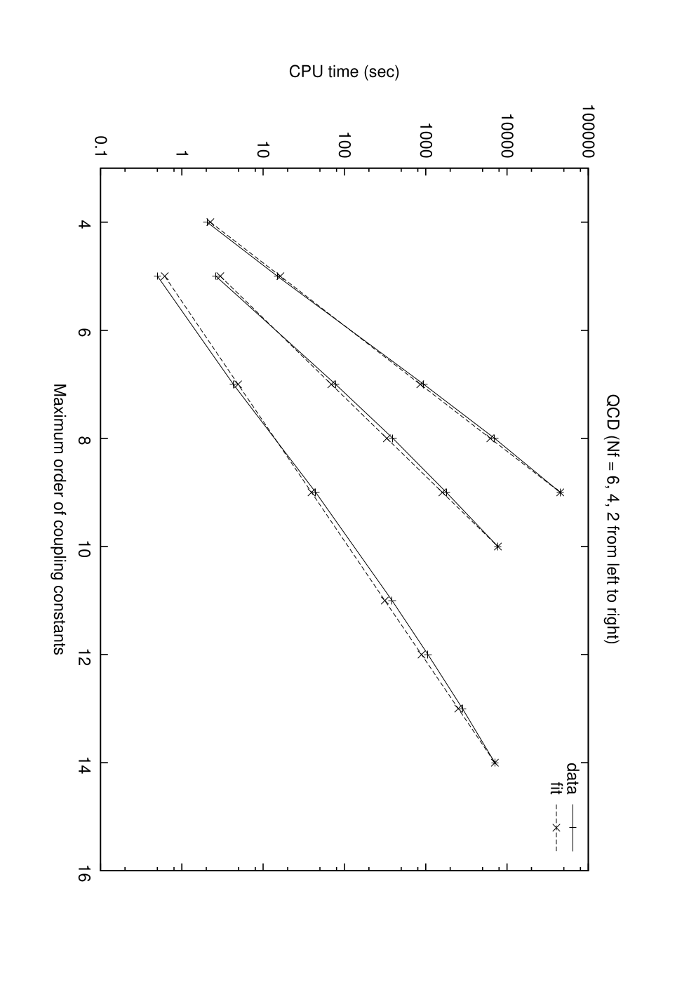
We have measured CPU time consumed for $N_{f}=2$ , $4$ , $6$ as shown in Fig. 1. It shows used CPU time grows exponentially for the order of coupling constants. The rate of the growth becomes steeper as increasing the number of fields.

Similar to the case of $\phi^{3}+\phi^{4}$ model, counter terms are included as shown in the same tables in Appendix C. The action is:

\begin{split}S&=\frac{1}{2}A^{2}+\sum_{j=1}^{N_{f}}\psi_{j}^{\prime*}\psi_{j}^{\prime}+\psi_{g}^{\prime*}\psi_{g}^{\prime}\\ &\quad-\Bigl(\sum_{n=0}g^{2n}\Bigr)\Bigl(\frac{g^{2}}{2}A^{2}+\sum_{j=1}^{N_{f}}g^{2}\psi_{j}^{\prime*}\psi_{j}^{\prime}+g^{2}\psi_{g}^{\prime*}\psi_{g}^{\prime}\\ &\qquad+\frac{g}{3!}A^{3}+\frac{g^{2}}{4!}A^{4}+g\sum_{j=1}^{N_{f}}\psi_{j}^{\prime*}\psi_{j}^{\prime}A+g\psi_{g}^{\prime*}\psi_{g}^{\prime}A\Bigr)\\ &\quad+AJ+\sum_{j=1}^{N_{f}}(\psi_{j}^{\prime*}\eta_{j}^{\prime}+\eta_{j}^{\prime*}\psi_{j}^{\prime})+\psi_{g}^{\prime*}\eta_{g}^{\prime}+\eta_{g}^{\prime*}\psi_{g}^{\prime}.\end{split}

(47)

Refer to caption — Figure 1: Comparison of CPU time for calculating the number of Feynman graphs in QCD with $N_{f}=$ 2, 4, 6 without counter terms. Dashed lines show exponential fit as functions of the order of maximum coupling constant $C_{\text{max}}$ .

4.3 QED

For QED, the formulation is to be modified to incorporate Furry’s theorem as described by Ref.[8]. It is done by replacing $Z_{1}$ of Eq.(13) by

\displaystyle Z_{1}(J,\sigma)

\displaystyle=(1-e^{2}A^{2})^{-1/2}\exp\Bigl[\frac{\sigma}{1-eA}\Bigr]e^{J^{2}/2},

where $A$ corresponds to photon field, $J$ to its source field, and $\sigma=\eta^{\prime*}\eta^{\prime}$ to the source field of electron-positron pair, and $e$ is QED coupling constant. Since electron and positron fields are already integrated out, replacement of $\rho^{m}=(\psi^{\prime*}\psi^{\prime})^{m}$ by $\tilde{P}_{m}$ is not necessary. Although the expression of $Q$ alters, the succeeding procedure of counting connected and 1PI is the same. As mentioned in [8], symmetry factors in QED equal to 1 except for vacuum graphs. Our program used about 110 seconds for $C_{\text{max}}=21$ . Results agreed with Ref.[8].

5 Summary and Discussions

A method of calculating the number of Feynman graphs weighted by symmetry factors for connected and 1PI Feynman graphs is proposed. With this method we have calculated in several models, especially in QCD, with or without counter terms. This method is to calculate generating functional directly in 0-dimensional field theory. The calculation is performed using a computer algebra system. The main technical points are the replacement of product of differential operators by polynomials $P_{m}$ , $\tilde{P}_{m,n}$ and $\tilde{P}_{m}$ , and calculation of Legendre transformation by repeated substitutions of variables.

Based on the obtained numbers, systematic testing tool is prepared in Feynman graph generator grc described in Ref.[4].

We present some comments in order:

•

This method is suitable for automatization. Once an action of a model is given, calculating procedure of $Z$ , and then the weighted number of connected graphs and 1PI graphs, is model independent.
•

As the number of particles increases, the expression grows rapidly. The calculated generating function includes all possible physical processes only limited by the maximum number of order of coupling constants.

The total number of processes grows rapidly corresponding to the growth of the number of combinations of external particles of possible processes. For this reason, the calculation in electro-weak theory, which includes 20 field variables, caused a problem of calculation size. We have succeeded to calculate up to ${\cal O}(g^{3})$ ; however, it failed for higher order calculation in REDUCE system because of memory problems.
•

It is possible to count numbers for process by process as a generalization of the method described in Ref.[8] based on Dyson-Schwinger equation. One can write down corresponding recursion relation among Green’s functions based on a differential equation satisfied by $P_{m}$ and $\tilde{P}_{m,n}$ . This method is described in Appendix B. We can calculate Green’s function one by one for connected graphs. However, it will be necessary to follow the same procedure for Legendre transformation to obtain 1PI graphs. This method will become complicated for the models with many particles such as electro-weak theory.
•

The most CPU consuming part is one of calculating Legendre transformation. Optimization of this part will be depending on computer algebra system.

Acknowledgments

The author wish to express his thanks to the members of Computing Research Center in KEK for their support in his scientific activities.

Appendix A Polynomials $P_{m}$ , $\tilde{P}_{m,n}$ and $\tilde{P}_{m}$

We look into the polynomial $P_{m}$ , $\tilde{P}_{m,n}$ and $\tilde{P}_{m}$ introduced by Eqs.(21) – (23).

A.1 $P_{m}$ : neutral scalar fields

Let $P_{m}(x)$ be polynomials defined by:

\displaystyle P_{m}(x)=e^{-x^{2}/2}\frac{d^{m}}{dx^{m}}e^{x^{2}/2}\qquad(j=0,1,2,...).

(48)

Polynomials $P_{m}$ can be expressed by Hermite polynomials:¹¹ 1 The definition of $H_{m}$ is different among textbooks. We use $H_{n}(x)=(-1)^{n}e^{x^{2}}\frac{d^{n}~}{dx^{n}}e^{-x^{2}}$ [11].

\displaystyle P_{m}(x)

\displaystyle=\Bigl(\frac{i}{\sqrt{2}}\Bigr)^{m}H_{m}\Bigl(-\frac{i}{\sqrt{2}}x\Bigr).

(49)

Generating function is

\displaystyle e^{t^{2}/2+tx}=\sum_{m=0}^{\infty}P_{m}(x)\frac{t^{m}}{m!}.

(50)

The explicit form of $P_{m}$ is

	$\displaystyle P_{2n}(x)$	$\displaystyle=\sum_{j=0}^{n}\left(\hskip-3.00003pt\begin{array}[]{c}n\\ j\end{array}\hskip-3.00003pt\right)\frac{(2n-1)!!}{(2j-1)!!}x^{2j},$
	$\displaystyle P_{2n+1}(x)$	$\displaystyle=\sum_{j=0}^{n}\left(\hskip-3.00003pt\begin{array}[]{c}n\\ j\end{array}\hskip-3.00003pt\right)\frac{(2n+1)!!}{(2j+1)!!}x^{2j+1}.$

It is easy to see that $P_{m}$ satisfies the following relations.

	$\displaystyle P_{m+2}(x)=xP_{m+1}(x)+(m+1)p_{m}(x),$		(55)
	$\displaystyle\frac{dP_{m}(x)}{dx}=mP_{m-1}(x).$		(56)

Each of them satisfies the following differential equation:

\Bigl(\frac{d^{2}~}{dx^{2}}+x\frac{d~}{dx}-m\Bigr)P_{m}(x)=0,

(57)

with initial values at $x=0$ :

\begin{split}P_{2n}(0)=\frac{(2n)!}{2^{n}n!},&\qquad P_{2n}^{\prime}(0)=0,\\ P_{2n+1}(0)=0,&\qquad P_{2n+1}^{\prime}(0)=\frac{(2n+1)!}{2^{n}n!}.\end{split}

(58)

The first several of them are as the following:

\begin{split}P_{0}(x)&=1,\\ P_{1}(x)&=x,\\ P_{2}(x)&=x^{2}+1,\\ P_{3}(x)&=x^{3}+3x,\\ P_{4}(x)&=x^{4}+6x^{2}+3,\\ P_{5}(x)&=x^{5}+10x^{3}+15x,\\ P_{6}(x)&=x^{6}+15x^{4}+45x^{2}+15.\end{split}

(59)

When $P_{j}$ is substituted to Eq.(24), the terms of $P_{j}(x)$ correspond to the same order of coupling constants and the lower degree terms contribute to the processes with less numbers of external particles. This implies that these lower degree terms correspond to the contiributions from graphs with loops.

A.2 $\tilde{P}_{m,n}$ : complex scalar fields

We define $\tilde{P}$ by:

\displaystyle\tilde{P}_{m,n}(x,y):=e^{-xy}\frac{\partial^{m}~}{\partial x^{m}}\frac{\partial^{n}~}{\partial y^{n}}e^{xy}.

(60)

These polynomials are expressed by Laguerre polynomial $L_{n}^{\alpha}$ :²² 2 We use the definition $L_{n}^{\alpha}(x)=\frac{1}{n!}e^{x}x^{-\alpha}\frac{d^{n}~}{dx^{n}}e^{-x}x^{n+\alpha}$ . This is also called Sonin polynomial.

\displaystyle\tilde{P}_{m,n}(x,y)

\displaystyle=m!\,x^{n-m}L_{m}^{n-m}(-xy)=n!\,y^{m-n}L_{n}^{m-n}(-xy).

(61)

Generating function of them is

\displaystyle e^{st+xt+ys}=\sum_{m=0}^{\infty}\sum_{n=0}^{\infty}\tilde{P}_{m,n}(x,y)\frac{s^{m}}{m!}\frac{t^{n}}{n!}.

(62)

The explicit form is:

\displaystyle\tilde{P}_{m,n}(x,y)=\sum_{k=0}^{\min(m,n)}\frac{m!n!}{k!(m-k)!(n-k)!}x^{n-k}y^{m-k}.

(63)

They satisfy the following recursion relations:

	$\displaystyle\tilde{P}_{m,n}(x,y)=\frac{\partial\tilde{P}_{m-1,n}}{\partial x}+y\tilde{P}_{m-1,n}\qquad(m\geq 1,\;n\geq 0),$		(64)
	$\displaystyle\tilde{P}_{m,n}(x,y)=\frac{\partial\tilde{P}_{m,n-1}}{\partial y}+x\tilde{P}_{m,n-1}\qquad(m\geq 0,\;n\geq 1),$		(65)

and the following differential equations:

	$\displaystyle\Bigl(\frac{\partial^{2}~}{\partial x\partial y}+x\frac{\partial~}{\partial x}-n\Bigr)\tilde{P}_{m,n}(x,y)=0,$		(66)
	$\displaystyle\Bigl(\frac{\partial^{2}~}{\partial x\partial y}+y\frac{\partial~}{\partial y}-m\Bigr)\tilde{P}_{m,n}(x,y)=0,$		(67)

with initial values at the origin:

\begin{split}\tilde{P}_{m,n}(0,0)&=m!\delta_{m,n},\\ \frac{\partial\tilde{P}_{m,n}}{\partial x}(0,0)=n!\delta_{m+1,n},&\qquad\frac{\partial\tilde{P}_{m,n}}{\partial y}(0,0)=m!\delta_{m,n+1}.\end{split}

(68)

The first several of them are shown as the following:

\begin{array}[]{|c|cccc|}\hline\cr m\backslash n&0&1&2&3\\ \hline\cr 0&1&x&x^{2}&x^{3}\\ 1&y&xy+1&x^{2}y+2x&x^{3}y+3x^{2}\\ 2&y^{2}&xy^{2}+2y&x^{2}y^{2}+4xy+2&x^{3}y^{2}+6x^{2}y+6x\\ 3&y^{3}&xy^{3}+3y^{2}&x^{2}y^{3}+6xy^{2}+6y&x^{3}y^{3}+9x^{2}y^{2}+18xy+6\\ \hline\cr\end{array}

(69)

A.3 $\tilde{P}_{m}$ : pairs of charged fields

When particle number is conserved for charged particle, $\tilde{P}_{m,n}$ appear only in the following form, in which we use $z=xy$ :

\displaystyle\tilde{P}_{m}(z)

\displaystyle:=\tilde{P}_{m,m}(x,y)=\sum_{k=0}^{m}\frac{1}{k!}\left(\frac{m!}{(m-k)!}\right)^{2}z^{m-k}.

(70)

They satisfy the following recursion relation:

\displaystyle\tilde{P}_{m+1}(z)

\displaystyle=z\frac{d^{2}\tilde{P}_{m}(z)}{dz^{2}}+(1+2z)\frac{d\tilde{P}_{m}(z)}{dz}+(1+z)\tilde{P}_{m}(z),

(71)

and differential equation

\Bigl(x\frac{d^{2}~}{dx^{2}}+(x+1)\frac{d~}{dx}-k\Bigr)\tilde{P}_{k}(x)=0,

(72)

with initial values at the origin:

\displaystyle\tilde{P}_{m}(0)=m!,

\displaystyle\qquad\tilde{P}_{m}^{\prime}(0)=m!\,m.

(73)

The first several of them are shown as the following:

\begin{split}\tilde{P}_{0}(z)&=1,\\ \tilde{P}_{1}(z)&=z+1,\\ \tilde{P}_{2}(z)&=z^{2}+4z+2,\\ \tilde{P}_{3}(z)&=z^{3}+9z^{2}+18z+6,\\ \tilde{P}_{4}(z)&=z^{4}+16z^{3}+72z^{2}+96z+24,\\ \tilde{P}_{5}(z)&=z^{5}+25z^{4}+200z^{3}+600z^{2}+600z+120,\\ \tilde{P}_{6}(z)&=z^{6}+36z^{5}+450z^{4}+2400z^{3}+5400z^{2}+4320z+720.\end{split}

(74)

Appendix B Recursion relation among Green’s functions.

Let us consider a model consists of gluon and ghost, for simplicity. The interaction part of action $S_{\text{int}}$ is

\displaystyle S_{\text{int}}

\displaystyle=-\frac{g}{3!}(rA)^{3}-\frac{g^{2}}{4!}(rA)^{4}-g(s\psi^{*}\psi)(rA),

(75)

where $A$ , $\psi$ , and $\psi^{*}$ are scalar fields corresponding to gluon, ghost, and anti-ghost fields, respectively. We use variable $\rho$ for the product of $\psi^{*}\psi$ , and $J$ for the source field of $A$ and $\sigma$ for one of $\rho$ . The variables $r$ and $s$ are introduced to count the power of $A$ and $\rho$ , respectively. The generating function becomes

	$\displaystyle Z_{1}=e^{-S_{\text{int}}}Z_{0}=(1+Q)Z_{0},\qquad Z_{0}=\exp\Bigl(\frac{1}{2}J^{2}+\sigma\Bigr),$		(76)
	$\displaystyle W=\log Z_{1}=\log(1+Q)+\frac{1}{2}J^{2}+\sigma.$		(77)

Expanding $e^{-S_{\text{int}}}$ we obtain

	$\displaystyle Q$	$\displaystyle=\sum_{l=0}\sum_{m=0}\sum_{n=0}\frac{g^{l+2m+n}r^{3l+4m+n}s^{n}}{(3!)^{l}l!(4!)^{m}m!n!}Z_{0}^{-1}A^{3l+4m+n}\rho^{l}Z_{0}-1$		(78)
		$\displaystyle=\sum_{l=0}\sum_{m=0}\sum_{n=0}\frac{g^{l+2m+n}r^{3l+4m+n}s^{n}}{(3!)^{l}l!(4!)^{m}m!n!}P_{3l+4m+n}(J)\tilde{P}_{n}(\sigma)-1.$		(79)

Using Eqs.(57) and (72) we obtain the following differential equations for $Q$ :

	$\displaystyle\Bigl(\frac{\partial^{2}~}{\partial J^{2}}+J\frac{\partial~}{\partial J}-r\frac{\partial~}{\partial r}\Bigr)Q=0,$		(80)
	$\displaystyle\Bigl(\sigma\frac{\partial^{2}~}{\partial\sigma^{2}}+(\sigma+1)\frac{\partial~}{\partial\sigma}-s\frac{\partial~}{\partial s}\Bigr)Q=0.$		(81)

From these equations one can obtain differential equations for $Z_{1}$ . They correspond to a generalization of Dyson-Schwinger equation described in Ref.[8]. We also obtain differential equations satisfied by the generating function $W$ for connected graphs:

	$\displaystyle\frac{\partial^{2}W}{\partial J^{2}}+\Bigl(\frac{\partial W}{\partial J}\Bigr)^{2}-J\frac{\partial W}{\partial J}-r\frac{\partial W}{\partial r}-1=0,$		(82)
	$\displaystyle\sigma\frac{\partial^{2}W}{\partial\sigma^{2}}+\sigma\Bigl(\frac{\partial W}{\partial\sigma}\Bigr)^{2}+(1-\sigma)\frac{\partial W}{\partial\sigma}-s\frac{\partial W}{\partial s}-1=0.$		(83)

Let us define the following functions of $r$ and $s$ :

\displaystyle W^{(j,k)}:=\frac{\partial^{j+k+k}W}{\partial J^{j}\partial\psi^{*k}\partial\psi^{k}}\Bigr|_{J=\sigma=0}=k!\frac{\partial^{j+k}W}{\partial J^{j}\partial\sigma^{k}}\Bigr|_{J=\sigma=0}.

(84)

They become Green’s functions of connected graphs when $r=s=1$ . We obtain recursion relation between $W^{(j,k)}$ from the differential equation of $W$ :

$\displaystyle W^{(2,0)}$	$\displaystyle=\frac{\partial~}{\partial r}W^{(0,0)}-(W^{(0,0)})^{2}+1,$	(85)
$\displaystyle W^{(0,1)}$	$\displaystyle=\frac{\partial~}{\partial r}W^{(0,0)}+1,$	(86)
$\displaystyle W^{(j+2,0)}$	$\displaystyle=\Bigl(r\frac{\partial~}{\partial r}+j\Bigr)W^{(j,0)}-\sum_{l=0}^{j}\left(\hskip-3.00003pt\begin{array}[]{c}j\\ l\end{array}\hskip-3.00003pt\right)W^{(l+1,0)}\,W^{(j-l+1,0)}\qquad(j\geq 1),$
$\displaystyle\begin{split}W^{(j,k+1)}&=\Bigl(s\frac{\partial~}{\partial s}+k\Bigr)W^{(j,k)}-\frac{k}{k+1}\sum_{l=0}^{k-1}\sum_{m=0}^{j}\left(\hskip-3.00003pt\begin{array}[]{c}k-1\\ l\end{array}\hskip-3.00003pt\right)\left(\hskip-3.00003pt\begin{array}[]{c}j\\ m\end{array}\hskip-3.00003pt\right)\\ &\quad\times\left(\hskip-3.00003pt\begin{array}[]{c}k+1\\ l+1\end{array}\hskip-3.00003pt\right)W^{(m,l+1)}\,W^{(j-m,k-l)}\qquad(j\geq 0,\quad k\geq 1).\end{split}$		(89)

This set of equations implies that all of $W^{(j,k)}$ can be obtained as functions of $r$ and $s$ with $W^{(0,0)}$ and $W^{(1,0)}$ as inputs. Let

\displaystyle Q^{(0,0)}=Q\Bigl|_{J=\sigma=0},\qquad Q^{(1,0)}=\frac{\partial Q}{\partial J}\Bigl|_{J=\sigma=0}.

(90)

They are functions of $r$ and $s$ of ${\cal O}(g)$ and are calculable from Eqs.(79), (58), and (73). Expanding with respect to the coupling constant $g$ , input functions $W^{(0,0)}$ and $W^{(1,0)}$ are calculable form:

	$\displaystyle W^{(0,0)}$	$\displaystyle=\log(1+Q^{(0,0)})=\sum_{l=1}\frac{(-1)^{l+1}}{l}{Q^{(0,0)}}^{l},$		(91)
	$\displaystyle W^{(1,0)}$	$\displaystyle=\frac{Q^{(1,0)}}{1+Q^{(0,0)}}=Q^{(1,0)}\sum_{l=0}(-1)^{l}{Q^{(0,0)}}^{l}.$		(92)

This method makes the problem size smaller, since it enables to calculate specific processes without calculating all possible processes. For 1PI graphs, however, one has to take the same procedure described in section 3.

It is straight forward to include other interaction terms such as counter terms. In these cases differential equations left unchanged; only $Q^{(0,0)}$ and $Q^{(1,0)}$ are changed through replacement of Eq.(79). It is also easy to include quarks by augmenting the number of charged scalars and replacing interaction term $g(s\psi^{*}\psi)(rA)$ by $g\sum_{i}(s_{i}\psi_{i}^{*}\psi_{i})(rA)$ . For more complicated model, it will be necessary to use differential equations for $\tilde{P}_{m,n}(x,y)$ and initial values given by Eqs.(66) – (68).

Appendix C Calculated numbers of Feynman graphs

Here we show the calculated numbers of Feynman graphs weighted by symmetry factor are shown in the following tables for scalar theory and QCD.³³ 3 More detailed numbers are available from http://research-up.kek.jp/people/kaneko/.

C.1 Scalar model $\phi^{3}+\phi^{4}$

The weighted number of Feynman graphs are shown for $\phi^{3}+\phi^{4}$ model in Table 1 for both with and without counter terms described by Eqs.(44) and (45). Column ‘E’ represents the number of external particles and ‘L’ the number of loops. Columns with ’(CT)’ indicate that counter terms are included in the model. Calculation was done for $C_{\text{max}}=21$ and the numbers were obtained from ( $\text{E}=0$ , $\text{L}=11$ ) to ( $\text{E}=23$ , $\text{L}=0$ ). However we show here a part of them limiting to $\text{E}\leq 6$ and $\text{L}\leq 7$ .

E	L	connected	1PI	conn. (CT)	1PI (CT)
0	2	$\displaystyle\frac{\displaystyle{1}}{\displaystyle{3}}$	$\displaystyle\frac{\displaystyle{5}}{\displaystyle{24}}$	$\displaystyle\frac{\displaystyle{5}}{\displaystyle{6}}$	$\displaystyle\frac{\displaystyle{17}}{\displaystyle{24}}$
0	3	$\displaystyle\frac{\displaystyle{11}}{\displaystyle{12}}$	$\displaystyle\frac{\displaystyle{7}}{\displaystyle{16}}$	$\displaystyle\frac{\displaystyle{37}}{\displaystyle{12}}$	$\displaystyle\frac{\displaystyle{95}}{\displaystyle{48}}$
0	4	$\displaystyle\frac{\displaystyle{1493}}{\displaystyle{288}}$	$\displaystyle\frac{\displaystyle{83}}{\displaystyle{36}}$	$\displaystyle\frac{\displaystyle{5441}}{\displaystyle{288}}$	$\displaystyle\frac{\displaystyle{685}}{\displaystyle{72}}$
0	5	$\displaystyle\frac{\displaystyle{25241}}{\displaystyle{576}}$	$\displaystyle\frac{\displaystyle{22235}}{\displaystyle{1152}}$	$\displaystyle\frac{\displaystyle{1345}}{\displaystyle{8}}$	$\displaystyle\frac{\displaystyle{86915}}{\displaystyle{1152}}$
0	6	$\displaystyle\frac{\displaystyle{50936927}}{\displaystyle{103680}}$	$\displaystyle\frac{\displaystyle{139829}}{\displaystyle{640}}$	$\displaystyle\frac{\displaystyle{40568905}}{\displaystyle{20736}}$	$\displaystyle\frac{\displaystyle{1631659}}{\displaystyle{1920}}$
0	7	$\displaystyle\frac{\displaystyle{284251517}}{\displaystyle{41472}}$	$\displaystyle\frac{\displaystyle{64155409}}{\displaystyle{20736}}$	$\displaystyle\frac{\displaystyle{581444297}}{\displaystyle{20736}}$	$\displaystyle\frac{\displaystyle{252924091}}{\displaystyle{20736}}$
E	L	connected	1PI	conn. (CT)	1PI (CT)
1	1	$\displaystyle\frac{\displaystyle{1}}{\displaystyle{2}}$	$\displaystyle\frac{\displaystyle{1}}{\displaystyle{2}}$	$\displaystyle\frac{\displaystyle{1}}{\displaystyle{2}}$	$\displaystyle\frac{\displaystyle{1}}{\displaystyle{2}}$
1	2	$\displaystyle\frac{\displaystyle{31}}{\displaystyle{24}}$	$\displaystyle\frac{\displaystyle{2}}{\displaystyle{3}}$	$\displaystyle\frac{\displaystyle{67}}{\displaystyle{24}}$	$\displaystyle\frac{\displaystyle{5}}{\displaystyle{3}}$
1	3	$\displaystyle\frac{\displaystyle{341}}{\displaystyle{48}}$	$\displaystyle\frac{\displaystyle{25}}{\displaystyle{8}}$	$\displaystyle\frac{\displaystyle{965}}{\displaystyle{48}}$	$\displaystyle\frac{\displaystyle{215}}{\displaystyle{24}}$
1	4	$\displaystyle\frac{\displaystyle{22949}}{\displaystyle{384}}$	$\displaystyle\frac{\displaystyle{76}}{\displaystyle{3}}$	$\displaystyle\frac{\displaystyle{73421}}{\displaystyle{384}}$	$\displaystyle\frac{\displaystyle{227}}{\displaystyle{3}}$
1	5	$\displaystyle\frac{\displaystyle{1545307}}{\displaystyle{2304}}$	$\displaystyle\frac{\displaystyle{41099}}{\displaystyle{144}}$	$\displaystyle\frac{\displaystyle{5329007}}{\displaystyle{2304}}$	$\displaystyle\frac{\displaystyle{128363}}{\displaystyle{144}}$
1	6	$\displaystyle\frac{\displaystyle{777673801}}{\displaystyle{82944}}$	$\displaystyle\frac{\displaystyle{194791}}{\displaystyle{48}}$	$\displaystyle\frac{\displaystyle{2826926677}}{\displaystyle{82944}}$	$\displaystyle\frac{\displaystyle{1912765}}{\displaystyle{144}}$
1	7	$\displaystyle\frac{\displaystyle{8665279117}}{\displaystyle{55296}}$	$\displaystyle\frac{\displaystyle{119528647}}{\displaystyle{1728}}$	$\displaystyle\frac{\displaystyle{98228574175}}{\displaystyle{165888}}$	$\displaystyle\frac{\displaystyle{408521413}}{\displaystyle{1728}}$
E	L	connected	1PI	conn. (CT)	1PI (CT)
2	1	$\displaystyle\frac{\displaystyle{3}}{\displaystyle{2}}$	$1$	$\displaystyle\frac{\displaystyle{5}}{\displaystyle{2}}$	$2$
2	2	$\displaystyle\frac{\displaystyle{25}}{\displaystyle{3}}$	$\displaystyle\frac{\displaystyle{41}}{\displaystyle{12}}$	$\displaystyle\frac{\displaystyle{55}}{\displaystyle{3}}$	$\displaystyle\frac{\displaystyle{89}}{\displaystyle{12}}$
2	3	$\displaystyle\frac{\displaystyle{1741}}{\displaystyle{24}}$	$\displaystyle\frac{\displaystyle{55}}{\displaystyle{2}}$	$\displaystyle\frac{\displaystyle{4511}}{\displaystyle{24}}$	$\displaystyle\frac{\displaystyle{739}}{\displaystyle{12}}$
2	4	$\displaystyle\frac{\displaystyle{80299}}{\displaystyle{96}}$	$\displaystyle\frac{\displaystyle{15275}}{\displaystyle{48}}$	$\displaystyle\frac{\displaystyle{77877}}{\displaystyle{32}}$	$\displaystyle\frac{\displaystyle{12445}}{\displaystyle{16}}$
2	5	$\displaystyle\frac{\displaystyle{6869123}}{\displaystyle{576}}$	$\displaystyle\frac{\displaystyle{167831}}{\displaystyle{36}}$	$\displaystyle\frac{\displaystyle{3624397}}{\displaystyle{96}}$	$\displaystyle\frac{\displaystyle{1785215}}{\displaystyle{144}}$
2	6	$\displaystyle\frac{\displaystyle{4192377457}}{\displaystyle{20736}}$	$\displaystyle\frac{\displaystyle{15668327}}{\displaystyle{192}}$	$\displaystyle\frac{\displaystyle{14127753307}}{\displaystyle{20736}}$	$\displaystyle\frac{\displaystyle{134370073}}{\displaystyle{576}}$
2	7	$\displaystyle\frac{\displaystyle{54906861275}}{\displaystyle{13824}}$	$\displaystyle\frac{\displaystyle{713735831}}{\displaystyle{432}}$	$\displaystyle\frac{\displaystyle{145437685477}}{\displaystyle{10368}}$	$\displaystyle\frac{\displaystyle{8671673855}}{\displaystyle{1728}}$
E	L	connected	1PI	conn. (CT)	1PI (CT)
3	0	$1$	$1$	$1$	$1$
3	1	$\displaystyle\frac{\displaystyle{15}}{\displaystyle{2}}$	$\displaystyle\frac{\displaystyle{5}}{\displaystyle{2}}$	$\displaystyle\frac{\displaystyle{23}}{\displaystyle{2}}$	$\displaystyle\frac{\displaystyle{7}}{\displaystyle{2}}$
3	2	$\displaystyle\frac{\displaystyle{1777}}{\displaystyle{24}}$	$\displaystyle\frac{\displaystyle{89}}{\displaystyle{4}}$	$\displaystyle\frac{\displaystyle{3541}}{\displaystyle{24}}$	$\displaystyle\frac{\displaystyle{141}}{\displaystyle{4}}$
3	3	$\displaystyle\frac{\displaystyle{44177}}{\displaystyle{48}}$	$\displaystyle\frac{\displaystyle{2265}}{\displaystyle{8}}$	$\displaystyle\frac{\displaystyle{104893}}{\displaystyle{48}}$	$\displaystyle\frac{\displaystyle{4207}}{\displaystyle{8}}$
3	4	$\displaystyle\frac{\displaystyle{5292685}}{\displaystyle{384}}$	$\displaystyle\frac{\displaystyle{214865}}{\displaystyle{48}}$	$\displaystyle\frac{\displaystyle{4746983}}{\displaystyle{128}}$	$\displaystyle\frac{\displaystyle{454181}}{\displaystyle{48}}$
3	5	$\displaystyle\frac{\displaystyle{556813237}}{\displaystyle{2304}}$	$\displaystyle\frac{\displaystyle{665317}}{\displaystyle{8}}$	$\displaystyle\frac{\displaystyle{1642681493}}{\displaystyle{2304}}$	$\displaystyle\frac{\displaystyle{3123995}}{\displaystyle{16}}$
3	6	$\displaystyle\frac{\displaystyle{403304188435}}{\displaystyle{82944}}$	$\displaystyle\frac{\displaystyle{112879507}}{\displaystyle{64}}$	$\displaystyle\frac{\displaystyle{1274880793255}}{\displaystyle{82944}}$	$\displaystyle\frac{\displaystyle{288922967}}{\displaystyle{64}}$
3	7	$\displaystyle\frac{\displaystyle{6112916597549}}{\displaystyle{55296}}$	$\displaystyle\frac{\displaystyle{72481379183}}{\displaystyle{1728}}$	$\displaystyle\frac{\displaystyle{20367609554609}}{\displaystyle{55296}}$	$\displaystyle\frac{\displaystyle{99633977599}}{\displaystyle{864}}$
E	L	connected	1PI	conn. (CT)	1PI (CT)
4	0	$4$	$1$	$4$	$1$
4	1	$57$	$\displaystyle\frac{\displaystyle{21}}{\displaystyle{2}}$	$83$	$\displaystyle\frac{\displaystyle{23}}{\displaystyle{2}}$
4	2	$\displaystyle\frac{\displaystyle{5057}}{\displaystyle{6}}$	$\displaystyle\frac{\displaystyle{709}}{\displaystyle{4}}$	$\displaystyle\frac{\displaystyle{9431}}{\displaystyle{6}}$	$\displaystyle\frac{\displaystyle{977}}{\displaystyle{4}}$
4	3	$\displaystyle\frac{\displaystyle{167621}}{\displaystyle{12}}$	$\displaystyle\frac{\displaystyle{26625}}{\displaystyle{8}}$	$\displaystyle\frac{\displaystyle{93098}}{\displaystyle{3}}$	$\displaystyle\frac{\displaystyle{43887}}{\displaystyle{8}}$
4	4	$\displaystyle\frac{\displaystyle{25097635}}{\displaystyle{96}}$	$\displaystyle\frac{\displaystyle{1112795}}{\displaystyle{16}}$	$\displaystyle\frac{\displaystyle{63396679}}{\displaystyle{96}}$	$\displaystyle\frac{\displaystyle{2109847}}{\displaystyle{16}}$
4	5	$\displaystyle\frac{\displaystyle{3167606597}}{\displaystyle{576}}$	$\displaystyle\frac{\displaystyle{12851447}}{\displaystyle{8}}$	$\displaystyle\frac{\displaystyle{183533261}}{\displaystyle{12}}$	$\displaystyle\frac{\displaystyle{54607215}}{\displaystyle{16}}$
4	6	$\displaystyle\frac{\displaystyle{2675975185651}}{\displaystyle{20736}}$	$\displaystyle\frac{\displaystyle{2606881563}}{\displaystyle{64}}$	$\displaystyle\frac{\displaystyle{8007976663465}}{\displaystyle{20736}}$	$\displaystyle\frac{\displaystyle{6084522087}}{\displaystyle{64}}$
4	7	$\displaystyle\frac{\displaystyle{46342382319659}}{\displaystyle{13824}}$	$\displaystyle\frac{\displaystyle{72138266309}}{\displaystyle{64}}$	$\displaystyle\frac{\displaystyle{73377025565557}}{\displaystyle{6912}}$	$\displaystyle\frac{\displaystyle{273097894951}}{\displaystyle{96}}$
E	L	connected	1PI	conn. (CT)	1PI (CT)
5	1	$\displaystyle\frac{\displaystyle{1149}}{\displaystyle{2}}$	$57$	$\displaystyle\frac{\displaystyle{1609}}{\displaystyle{2}}$	$57$
5	2	$\displaystyle\frac{\displaystyle{280735}}{\displaystyle{24}}$	$1660$	$\displaystyle\frac{\displaystyle{497755}}{\displaystyle{24}}$	$2110$
5	3	$\displaystyle\frac{\displaystyle{11848865}}{\displaystyle{48}}$	$43890$	$\displaystyle\frac{\displaystyle{8320755}}{\displaystyle{16}}$	$66380$
5	4	$\displaystyle\frac{\displaystyle{2154582745}}{\displaystyle{384}}$	$1181335$	$\displaystyle\frac{\displaystyle{1721661675}}{\displaystyle{128}}$	$2056895$
5	5	$\displaystyle\frac{\displaystyle{319917889435}}{\displaystyle{2304}}$	$\displaystyle\frac{\displaystyle{533959855}}{\displaystyle{16}}$	$\displaystyle\frac{\displaystyle{846167432375}}{\displaystyle{2304}}$	$\displaystyle\frac{\displaystyle{1045018815}}{\displaystyle{16}}$
5	6	$\displaystyle\frac{\displaystyle{310780872308809}}{\displaystyle{82944}}$	$\displaystyle\frac{\displaystyle{8002786883}}{\displaystyle{8}}$	$\displaystyle\frac{\displaystyle{886800014611093}}{\displaystyle{82944}}$	$2159061195$
5	7	$\displaystyle\frac{\displaystyle{6083474414980385}}{\displaystyle{55296}}$	$31945379025$	$\displaystyle\frac{\displaystyle{55258819995230675}}{\displaystyle{165888}}$	$\displaystyle\frac{\displaystyle{898253508065}}{\displaystyle{12}}$
E	L	connected	1PI	conn. (CT)	1PI (CT)
6	1	$7230$	$390$	$9840$	$390$
6	2	$\displaystyle\frac{\displaystyle{1149515}}{\displaystyle{6}}$	$17865$	$\displaystyle\frac{\displaystyle{1958885}}{\displaystyle{6}}$	$21555$
6	3	$\displaystyle\frac{\displaystyle{59748815}}{\displaystyle{12}}$	$641025$	$10042310$	$908550$
6	4	$\displaystyle\frac{\displaystyle{12905505595}}{\displaystyle{96}}$	$21758395$	$\displaystyle\frac{\displaystyle{29598249775}}{\displaystyle{96}}$	$35376685$
6	5	$\displaystyle\frac{\displaystyle{2219089049855}}{\displaystyle{576}}$	$\displaystyle\frac{\displaystyle{5931760395}}{\displaystyle{8}}$	$\displaystyle\frac{\displaystyle{312229182035}}{\displaystyle{32}}$	$\displaystyle\frac{\displaystyle{10838888715}}{\displaystyle{8}}$
6	6	$\displaystyle\frac{\displaystyle{2449771948135225}}{\displaystyle{20736}}$	$\displaystyle\frac{\displaystyle{208155635205}}{\displaystyle{8}}$	$\displaystyle\frac{\displaystyle{6703936630258195}}{\displaystyle{20736}}$	$52505971410$
6	7	$\displaystyle\frac{\displaystyle{53708019970406075}}{\displaystyle{13824}}$	$\displaystyle\frac{\displaystyle{7615451146345}}{\displaystyle{8}}$	$\displaystyle\frac{\displaystyle{117185488235187485}}{\displaystyle{10368}}$	$\displaystyle\frac{\displaystyle{8360116793335}}{\displaystyle{4}}$

Table 1 Table of weighted number in $\phi^{3}+\phi^{4}$ model, with and without counter terms for (external particles) $\leq 6$ and (loops) $\leq 7$ . ‘E’ represents the number of external particles and ‘L’ the number of loops. Symbol ‘(CT)’ indicates that counter terms are included in the model.

C.2 QCD with six quarks

The weighted number of Feynman graphs is shown for QCD with six quarks $N_{f}=6$ in Table 2 for both with and without counter terms. Column ‘E’ represents the number of external particles, ‘L’ the number of loops, ‘ $gl$ ’, ‘ $q_{1}$ ’ and ‘ $q_{2}$ ’ are the number of external gluons, first and second quarks. We show only for the case of $q_{3}=q_{4}=q_{5}=q_{6}=0$ . By renumbering quarks one obtains numbers for some other combinations. It is calculated for $C_{\text{max}}=9$ and the number is obtained from ( $\text{E}=0$ , $\text{L}=5$ ) to ( $\text{E}=11$ , $\text{L}=0$ ). However we show here limiting to $\text{E}\leq 4$ .

E	L	$gl$	$q_{1}$	$q_{2}$	connected	1PI	conn. (CT)	1PI (CT)
0	2	0	0	0	$\displaystyle\frac{\displaystyle{191}}{\displaystyle{6}}$	$\displaystyle\frac{\displaystyle{89}}{\displaystyle{24}}$	$\displaystyle\frac{\displaystyle{118}}{\displaystyle{3}}$	$\displaystyle\frac{\displaystyle{269}}{\displaystyle{24}}$
0	3	0	0	0	$\displaystyle\frac{\displaystyle{2417}}{\displaystyle{6}}$	$\displaystyle\frac{\displaystyle{1141}}{\displaystyle{48}}$	$573$	$\displaystyle\frac{\displaystyle{853}}{\displaystyle{16}}$
0	4	0	0	0	$\displaystyle\frac{\displaystyle{2597681}}{\displaystyle{288}}$	$\displaystyle\frac{\displaystyle{11465}}{\displaystyle{36}}$	$\displaystyle\frac{\displaystyle{3916397}}{\displaystyle{288}}$	$\displaystyle\frac{\displaystyle{45709}}{\displaystyle{72}}$
0	5	0	0	0	$\displaystyle\frac{\displaystyle{19226297}}{\displaystyle{72}}$	$\displaystyle\frac{\displaystyle{7313267}}{\displaystyle{1152}}$	$\displaystyle\frac{\displaystyle{245546135}}{\displaystyle{576}}$	$\displaystyle\frac{\displaystyle{14591195}}{\displaystyle{1152}}$
E	L	$gl$	$q_{1}$	$q_{2}$	connected	1PI	conn. (CT)	1PI (CT)
1	1	1	0	0	$\displaystyle\frac{\displaystyle{15}}{\displaystyle{2}}$	$\displaystyle\frac{\displaystyle{15}}{\displaystyle{2}}$	$\displaystyle\frac{\displaystyle{15}}{\displaystyle{2}}$	$\displaystyle\frac{\displaystyle{15}}{\displaystyle{2}}$
1	2	1	0	0	$\displaystyle\frac{\displaystyle{2383}}{\displaystyle{24}}$	$\displaystyle\frac{\displaystyle{67}}{\displaystyle{6}}$	$\displaystyle\frac{\displaystyle{2923}}{\displaystyle{24}}$	$\displaystyle\frac{\displaystyle{157}}{\displaystyle{6}}$
1	3	1	0	0	$\displaystyle\frac{\displaystyle{124199}}{\displaystyle{48}}$	$\displaystyle\frac{\displaystyle{3533}}{\displaystyle{24}}$	$\displaystyle\frac{\displaystyle{164807}}{\displaystyle{48}}$	$\displaystyle\frac{\displaystyle{6109}}{\displaystyle{24}}$
1	4	1	0	0	$\displaystyle\frac{\displaystyle{33696533}}{\displaystyle{384}}$	$\displaystyle\frac{\displaystyle{72421}}{\displaystyle{24}}$	$\displaystyle\frac{\displaystyle{15994703}}{\displaystyle{128}}$	$\displaystyle\frac{\displaystyle{123833}}{\displaystyle{24}}$
1	5	1	0	0	$\displaystyle\frac{\displaystyle{8024429617}}{\displaystyle{2304}}$	$\displaystyle\frac{\displaystyle{5842663}}{\displaystyle{72}}$	$\displaystyle\frac{\displaystyle{12200014181}}{\displaystyle{2304}}$	$\displaystyle\frac{\displaystyle{2605201}}{\displaystyle{18}}$
E	L	$gl$	$q_{1}$	$q_{2}$	connected	1PI	conn. (CT)	1PI (CT)
2	1	2	0	0	$\displaystyle\frac{\displaystyle{31}}{\displaystyle{2}}$	$8$	$\displaystyle\frac{\displaystyle{33}}{\displaystyle{2}}$	$9$
2	2	2	0	0	$\displaystyle\frac{\displaystyle{1621}}{\displaystyle{3}}$	$\displaystyle\frac{\displaystyle{587}}{\displaystyle{12}}$	$\displaystyle\frac{\displaystyle{1903}}{\displaystyle{3}}$	$\displaystyle\frac{\displaystyle{971}}{\displaystyle{12}}$
2	3	2	0	0	$\displaystyle\frac{\displaystyle{181157}}{\displaystyle{8}}$	$\displaystyle\frac{\displaystyle{4457}}{\displaystyle{4}}$	$\displaystyle\frac{\displaystyle{692233}}{\displaystyle{24}}$	$\displaystyle\frac{\displaystyle{9809}}{\displaystyle{6}}$
2	4	2	0	0	$\displaystyle\frac{\displaystyle{33883405}}{\displaystyle{32}}$	$\displaystyle\frac{\displaystyle{523703}}{\displaystyle{16}}$	$\displaystyle\frac{\displaystyle{46451897}}{\displaystyle{32}}$	$\displaystyle\frac{\displaystyle{2422249}}{\displaystyle{48}}$
2	1	0	2	0	$\displaystyle\frac{\displaystyle{17}}{\displaystyle{2}}$	$1$	$\displaystyle\frac{\displaystyle{19}}{\displaystyle{2}}$	$2$
2	2	0	2	0	$\displaystyle\frac{\displaystyle{4741}}{\displaystyle{24}}$	$11$	$\displaystyle\frac{\displaystyle{6013}}{\displaystyle{24}}$	$16$
2	3	0	2	0	$\displaystyle\frac{\displaystyle{101731}}{\displaystyle{16}}$	$\displaystyle\frac{\displaystyle{2489}}{\displaystyle{12}}$	$\displaystyle\frac{\displaystyle{139813}}{\displaystyle{16}}$	$\displaystyle\frac{\displaystyle{3821}}{\displaystyle{12}}$
2	4	0	2	0	$\displaystyle\frac{\displaystyle{281573453}}{\displaystyle{1152}}$	$\displaystyle\frac{\displaystyle{64357}}{\displaystyle{12}}$	$\displaystyle\frac{\displaystyle{415076813}}{\displaystyle{1152}}$	$\displaystyle\frac{\displaystyle{35201}}{\displaystyle{4}}$
E	L	$gl$	$q_{1}$	$q_{2}$	connected	1PI	conn. (CT)	1PI (CT)
3	0	3	0	0	$1$	$1$	$1$	$1$
3	1	3	0	0	$\displaystyle\frac{\displaystyle{141}}{\displaystyle{2}}$	$\displaystyle\frac{\displaystyle{33}}{\displaystyle{2}}$	$\displaystyle\frac{\displaystyle{149}}{\displaystyle{2}}$	$\displaystyle\frac{\displaystyle{35}}{\displaystyle{2}}$
3	2	3	0	0	$\displaystyle\frac{\displaystyle{101401}}{\displaystyle{24}}$	$\displaystyle\frac{\displaystyle{1097}}{\displaystyle{4}}$	$\displaystyle\frac{\displaystyle{116437}}{\displaystyle{24}}$	$\displaystyle\frac{\displaystyle{1485}}{\displaystyle{4}}$
3	3	3	0	0	$\displaystyle\frac{\displaystyle{12090827}}{\displaystyle{48}}$	$\displaystyle\frac{\displaystyle{79097}}{\displaystyle{8}}$	$\displaystyle\frac{\displaystyle{15005863}}{\displaystyle{48}}$	$\displaystyle\frac{\displaystyle{105231}}{\displaystyle{8}}$
3	4	3	0	0	$\displaystyle\frac{\displaystyle{5869833661}}{\displaystyle{384}}$	$\displaystyle\frac{\displaystyle{19132001}}{\displaystyle{48}}$	$\displaystyle\frac{\displaystyle{7831563637}}{\displaystyle{384}}$	$\displaystyle\frac{\displaystyle{27380549}}{\displaystyle{48}}$
3	0	1	2	0	$1$	$1$	$1$	$1$
3	1	1	2	0	$\displaystyle\frac{\displaystyle{69}}{\displaystyle{2}}$	$2$	$\displaystyle\frac{\displaystyle{77}}{\displaystyle{2}}$	$3$
3	2	1	2	0	$\displaystyle\frac{\displaystyle{8671}}{\displaystyle{6}}$	$\displaystyle\frac{\displaystyle{113}}{\displaystyle{2}}$	$\displaystyle\frac{\displaystyle{5303}}{\displaystyle{3}}$	$\displaystyle\frac{\displaystyle{139}}{\displaystyle{2}}$
3	3	1	2	0	$\displaystyle\frac{\displaystyle{1617019}}{\displaystyle{24}}$	$\displaystyle\frac{\displaystyle{3481}}{\displaystyle{2}}$	$\displaystyle\frac{\displaystyle{2140925}}{\displaystyle{24}}$	$2403$
3	4	1	2	0	$\displaystyle\frac{\displaystyle{488989393}}{\displaystyle{144}}$	$\displaystyle\frac{\displaystyle{1502905}}{\displaystyle{24}}$	$\displaystyle\frac{\displaystyle{695346481}}{\displaystyle{144}}$	$\displaystyle\frac{\displaystyle{2258617}}{\displaystyle{24}}$
E	L	$gl$	$q_{1}$	$q_{2}$	connected	1PI	conn. (CT)	1PI (CT)
4	0	4	0	0	$4$	$1$	$4$	$1$
4	1	4	0	0	$491$	$\displaystyle\frac{\displaystyle{105}}{\displaystyle{2}}$	$517$	$\displaystyle\frac{\displaystyle{107}}{\displaystyle{2}}$
4	2	4	0	0	$\displaystyle\frac{\displaystyle{259367}}{\displaystyle{6}}$	$\displaystyle\frac{\displaystyle{7513}}{\displaystyle{4}}$	$\displaystyle\frac{\displaystyle{293813}}{\displaystyle{6}}$	$\displaystyle\frac{\displaystyle{9125}}{\displaystyle{4}}$
4	3	4	0	0	$3406344$	$\displaystyle\frac{\displaystyle{803681}}{\displaystyle{8}}$	$\displaystyle\frac{\displaystyle{16607145}}{\displaystyle{4}}$	$\displaystyle\frac{\displaystyle{1003895}}{\displaystyle{8}}$
4	1	2	2	0	$\displaystyle\frac{\displaystyle{435}}{\displaystyle{2}}$	$7$	$\displaystyle\frac{\displaystyle{477}}{\displaystyle{2}}$	$7$
4	2	2	2	0	$\displaystyle\frac{\displaystyle{332795}}{\displaystyle{24}}$	$\displaystyle\frac{\displaystyle{741}}{\displaystyle{2}}$	$\displaystyle\frac{\displaystyle{397163}}{\displaystyle{24}}$	$\displaystyle\frac{\displaystyle{849}}{\displaystyle{2}}$
4	3	2	2	0	$\displaystyle\frac{\displaystyle{13902103}}{\displaystyle{16}}$	$\displaystyle\frac{\displaystyle{204421}}{\displaystyle{12}}$	$\displaystyle\frac{\displaystyle{53753347}}{\displaystyle{48}}$	$\displaystyle\frac{\displaystyle{263995}}{\displaystyle{12}}$
4	1	0	4	0	$111$	$4$	$125$	$4$
4	2	0	4	0	$5816$	$138$	$7212$	$170$
4	3	0	4	0	$\displaystyle\frac{\displaystyle{3747299}}{\displaystyle{12}}$	$\displaystyle\frac{\displaystyle{15763}}{\displaystyle{3}}$	$\displaystyle\frac{\displaystyle{1681643}}{\displaystyle{4}}$	$\displaystyle\frac{\displaystyle{21589}}{\displaystyle{3}}$
4	1	0	2	2	$\displaystyle\frac{\displaystyle{111}}{\displaystyle{2}}$	$2$	$\displaystyle\frac{\displaystyle{125}}{\displaystyle{2}}$	$2$
4	2	0	2	2	$2908$	$69$	$3606$	$85$
4	3	0	2	2	$\displaystyle\frac{\displaystyle{3747299}}{\displaystyle{24}}$	$\displaystyle\frac{\displaystyle{15763}}{\displaystyle{6}}$	$\displaystyle\frac{\displaystyle{1681643}}{\displaystyle{8}}$	$\displaystyle\frac{\displaystyle{21589}}{\displaystyle{6}}$

Table 2 Table of weighted number of QCD with 6 quarks, with and without counter terms. ‘E’ represents the number of external particles, ‘L’ the number of loops, ‘ $gl$ ’ the number of external gluons, and ‘ $q_{1}$ ’, ’ $q_{2}$ ’ the number of external quark 1, 2. Symbol ‘(CT)’ indicates that counter terms are included in the model.

References

[1] T.Sasaki, J. of Comput. Phys. 22 (1976) 189.
[2] T.Kaneko, S.Kawabata and Y.Shimizu, Comput. Phys. Commun. 43 (1987) 279.
[3] P.Nogueira, J. of Comput. Phys. 105 (1993) 279.
[4] T. Kaneko, Comput. Phys. Commun. 92 (1995) 127–152. The current version of Feynman graph generator grc is available from http://research-up.kek.jp/people/kaneko/.
[5] T. Hahn, Comput. Phys. Commun. 140 (2001) 418–431.
[6] J-X. Wang, NIMA 534 (2004) 241–245.
[7] F.Harary and E.M.Palmer, “Graphical Enumeration”, Academic Press, New York, 1973.
[8] P.Cvitanović, B.Lautrup, and R.B.Pearson, Phys. Rev. D18 (1978)1939.
[9] C.Itzykson and J.B.Zuber, “Quantum Field Theory”, McGraw-Hill, 1980; Dover, 2005.
[10] REDUCE, ‘A portable general-purpose computer algebra system’, http://reduce-algebra.sourceforge.net/.
[11] A. Erdelyi, et. al, ‘Higher transcendental functions, II’, Bateman Manuscript Project, McGaw-Hill, 1953.