Degenerate Zeeman Ground States in the Single-Excitation Regime

This work considers an ensemble of atoms interacting, via the dipole moments of an arbitrary $J_{g}\rightarrow J_{e}$ transition, with both a laser and the quantized electromagnetic field. Assuming the system is Markovian, we use the Lindblad form of the master equation for the reduced density matrix, $\hat{\rho}(t)$ [44, 45]:

Here $C^{q}_{M_{g}}\equiv\langle{J_{e}(M_{g}+q)}|1q;J_{g}M_{g}\rangle$ is a Clebsch-Gordon coefficient, $\sigma^{j+}_{M_{g}q}\equiv\ket{eJ_{e}(M_{g}+q)}_{j}\bra{gJ_{g}M_{g}}=(\sigma^{j-}_{M_{g}q})^{\dagger}$, $\Gamma$ is the single atom decay rate, $\alpha_{jj^{\prime}}\equiv k|\boldsymbol{r}_{j}-\boldsymbol{r}_{j^{\prime}}|$, and $g^{qq^{\prime}}_{jj^{\prime}}(\alpha_{jj^{\prime}})$ is the inelastic and elastic dipole-dipole Green’s function:

where $\hat{\boldsymbol{n}}_{jj^{\prime}}\equiv(\boldsymbol{r}_{j}-\boldsymbol{r}_{j^{\prime}})/|\boldsymbol{r}_{j}-\boldsymbol{r}_{j^{\prime}}|$, and $\hat{\boldsymbol{e}}_{q}$ represents the $q^{th}$ unit polarization vector. Using the rotating-wave approximation,

where $\Delta$ is the detuning of the laser, $\mathcal{D}$ is the reduced dipole matrix element [46], and $\boldsymbol{E}_{j}$ is the laser field for atom $j$.

In order to simulate such highly correlated systems, in this section, we will derive a hierarchy of operator expectation values using Eq. (1). Note that a physically equivalent, field theoretical, set of equations is presented in Ref. [11]. Here, we calculate the time dependence of the expectation value of the $\sigma^{j-}_{M_{g}q}$ operators using the equation:

This gives:

For this system, it is useful to probe the low-intensity ($|E||\mathcal{D}|\ll\Gamma\hbar$) limit. This allows one to set terms $\propto\sigma^{j+}_{M_{g}^{\prime}q^{\prime}}\sigma^{j-}_{M_{g}q}$ equal to zero, since these terms only project onto states with excited atoms. Further, we consider only the case where the system is initially in an uncorrelated mixed state. This may be simulated by stochastically assigning each atom a Zeeman ground state, $M_{g}^{j}$, and then averaging over many runs [6, 11]. This allows us to make the approximation $\langle\sigma^{j-}_{M_{g}^{\prime}q^{\prime}}\sigma^{j+}_{M_{g}q}\rangle\rightarrow\delta_{M_{g}^{\prime}M_{g}}\delta_{qq^{\prime}}\delta_{M_{g}M^{j}_{g}}$, since the developement of correlations between different $M_{g}$ values, for states with only ground state atoms, is increasingly slow in the low-intensity limit. Considering these approximations gives:

In order to solve for the one atom correlation operators, one must solve for the two atom correlation operators, then the three atom correlation operators, etc… This produces a hierarchy of equations that grows exponentially with $N$. Because of this, the expectation values of the correlation functions are often factorized in the following way:

keeping in mind that we have stochastically assigned a value of $M_{g}^{j}$ to each atom. This gives:

The approximate equations above are the ones typically used [9, 18, 19, 6, 5], and are exact when $J_{g}=0$ and $J_{e}=1$ [9]. The factorized terms in Eq. (7) are often highly correlated for dense systems, making this approximation inadequate. In fact, as will be demonstrated in Sec. III, their presence changes the system’s photon scattering in non-trivial ways. A technique capable of addressing these correlations, while remaining computationally pragmatic, is required.

In this section, we develop a system of equations capable of addressing the correlations that emerge in Eq. (1), in the low-intensity limit. An alternate, yet physically equivalent, set of equations is presented in Ref. [11]. First, we write the density matrix in the following way:

Here, $e$ represents the number of excitations in a given state, and $m$ is an index that runs over all the states within that subspace. We assume that the system is initialized in the pure state $\ket{0,g}$ and subsequently driven by a low-intensity laser. In the low-intensity limit:

We also note that the rate of population transfer is $\propto c_{1,m;1,n}\Gamma$, while the system approaches a quasi-steady state at a rate $\propto\Gamma$. Therefore, we neglect the effects of population transfer, i.e. terms in Eq. (1) $\propto\sigma^{j-}_{M_{g}q}\hat{\rho}(t)\sigma^{j^{\prime}+}_{M_{g}^{\prime}q^{\prime}}$. Considering this, Eq. (1) shows that the $c_{0,g;0,g}$ density matrix element only couples to the $c_{1,m;0,g}$ elements, as well as their complex conjugates. Also, to first order, the $c_{1,m;0,g}$ density matrix elements are only coupled to the $c_{0,g;0,g}$, as well as the $c_{1,n;0,g}$ elements. The relevant space of density matrix elements only couples to states with $\bra{0,g}$ as the column state, therefore, the rows and the columns of the density matrix are completely uncorrelated, allowing us to rewrite $\hat{\rho}(t)$ as:

dramatically reducing the number of independent complex numbers needed to describe the density matrix. Further, in the low-intensity limit, the following properties are true:

Considering the above approximations:

which allows one to construct any physical quantities $\propto c_{1m}(t)c^{*}_{1,n}(t)$, such as the photon scattering rate, from the significantly smaller subspace of $c_{1,m}(t)c^{*}_{0,g}(t)\simeq c_{1,m}(t)$ density matrix elements. Note that the $c_{1,m}(t)c_{0,g}^{*}(t)$ terms will be labeled simply $c_{1,m}(t)$ from now on. Resultantly, we may solve for the system’s dynamics from the $c_{1,m}(t)$ subspace, tracking only the operations on the left side of $\hat{\rho}(t)$. This gives:

The amount of elements in this subspace is $N(2J_{e}+1)(2J_{g}+1)^{N-1}$, which is considerably less than the $4^{N}(J_{e}+J_{g}+1)^{2N}$ elements in the full density matrix. This allows us to simulate clouds of significantly more atoms, while still including the relevant correlations present in systems with $J_{g}\neq 0$. An interesting feature of Eq. (II.3) is that it is equivalent to Eq. (II.2) for ensembles of $J_{g}=0\rightarrow J_{e}=1$ atoms. For this angular momentum structure, both approaches are exact in the low-intensity regime, and are equivalent to the coupled harmonic oscillator approach typically used in the literature [2, 3, 4, 5, 6, 7, 8, 9, 10, 11, 12, 18, 19, 21, 22, 40]. This indicates that Eq. (II.3) may be viewed as a generalization to these equations.

Equation (II.3) approaches exactness in the limit where the system scatters a single real photon. This is shown in Fig. 1. Here, we compare calculations of the photon scattering rate, $\gamma$, for individual configurations of dense clouds of $4$ $J_{g}=1/2$, $J_{e}=1/2$ atoms driven by a plane wave laser. In this figure, it is shown that for larger Rabi frequencies, the photon scattering rate obtained using Eq. (1) yields different results than Eq. (II.3). However, for lower intensity lasers the two calculations are equivalent. Fig. 1 also demonstrates that simulations using Eq. (II.2) and Eq. (II.3) produce different photon scattering rates, even at low laser intensities. Note that the results from Eq. (II.3) approach the exact result (i.e. Eq. (1)) while Eq. (II.2) does not. Equation (II.3) has the capacity to simulate much larger ensembles than Eq. (1). This is demonstrated in Fig. 2, where $\gamma$ for a cloud of $16$ atoms is calculated. Simulations with this many atoms are not possible when using Eq. (1), since the number of elements in the density matrix is more than $10^{13}$ times larger than the number required to use Eq. (II.3).

While Eq. (II.3) allows one to simulate clouds containing significantly more atoms than Eq. (1) does, its computational capacity falls short of the ability to simulate clouds containing hundreds of atoms. Since this regime is that of recent experiments [6, 9], an algorithm that can both simulate hundreds of atoms, and still keep the most relevant correlations, is needed. In order to accomplish this, we truncate the set of terms that Eq. (II.3) spans.

First, the system is stochastically assigned the pure state with $0$ excitations, labeled $\ket{0,g}$. Here, and in the rest of this work, we assume a $\hat{\boldsymbol{z}}$ polarized laser. Upon a given initialization, the set of $c_{1,n}\ket{1,n}\bra{0,g}$ obtained through all permutations of the following operation is kept:

while all other terms are set to $0$. In words, we keep the terms that are obtainable through an absorption of a single $\hat{\boldsymbol{z}}$ polarized photon from the laser, as well as the states obtainable through the exchange of one photon between atoms. This is useful because the size of the relevant space scales $\propto N^{2}$ as opposed to exponentially. Unlike Eq. (II.3), this algorithm’s scaling with $N$ is independent of the level-structure of the system, allowing for the simulation of large clouds of atoms with complex angular momentum structures. The following sections demonstrate that these approximations yield accurate results in many relevant systems.

The collective nature of dipole-dipole interactions in a one dimensional array has been shown to produce non-trivial radiative properties [19, 40, 9, 31]. For this system, we show the importance of correlations between degenerate Zeeman ground states by demonstrating their effect on the photon scattering of an array containing $J_{g}=1/2\rightarrow J_{e}=1/2$ atoms. Here the array is aligned along the $\hat{\boldsymbol{y}}$ direction, while the laser is a plane wave propagating along the $\hat{\boldsymbol{x}}$ direction and polarized in the $\hat{\boldsymbol{z}}$ direction. All of the results here are for an initially uncorrelated mixuture of Zeeman ground states, where every value of $M_{g}$ has an equal probability. For all the calculations shown, this is simulated by stochastically averaging over 320 runs where every atom is assigned a random value of $M_{g}$.

The results from Eq. (II.3) are compared with the results from both Eq. (II.2) and Eq. (15). This is, to some extent, a good quantification of the importance of correlations in the photon scattering process. Equation (II.3) contains correlations between Zeeman states to all orders, Eq. (15) only includes the correlations resulting from a single virtual photon exchange between states, while Eq. (II.2) contains none of these correlations.

Figure 3 compares the steady-state photon scattering rate, $\gamma$, versus detuning $\Delta$ for an array of atoms using Eq. (II.2), Eq. (15), and Eq. (II.3). In the figure, it is seen that for array spacings of $0.6\lambda$, the photon scattering lineshape is equivalent using all three methods. This indicates that in this regime, higher order correlations do not play a significant role in the system. Since the rate of virtual photon exchanges between states is $\propto 1/\delta r^{3}$, for smaller array spacings, correlations develop and the photon scattering lineshapes given by the three methods become qualitatively different. This is shown in Fig. 3, where for array spacings of $\delta r=0.2\lambda$, the lineshape calculated using Eq. (II.2) is still a Lorentzian structure, while the lineshapes calculated using both Eq. (II.3) and Eq. (15) have deviated from a Lorentzian shape, clearly forming double peaked structures. The figure demonstrates that for this value of $\delta r$, many of the differences between Eq. (II.2) and Eq. (II.3) can be explained by the first-order correlations given by Eq. (15), since two the calculations produce similar results. For even smaller array spacings, however, the results between all three calculations qualitatively differ. This is indicative of the fact that, here, even higher order correlations need to be included.

In this section, we calculate the lineshape of the scattered radiation from a Gaussian cloud, with an average density $\mathcal{N}=\frac{N}{\sigma_{x}\sigma_{y}\sigma_{z}(4\pi)^{3/2}}$ and a distribution:

driven by a plane wave laser polarized in the $\hat{\boldsymbol{z}}$ direction. This system is of particular interest due to recent experiments on cold clouds of ⁸⁷Rb [6, 9]. ⁸⁷Rb has two hyperfine ground states: $(5S_{1/2}F=1)$ and $(5S_{1/2}F=2)$. In these two experiments, the atoms are optically pumped into the $(5S_{1/2}F=2)$ ground state, and the closed transition to the $(5P_{3/2}F=3)$ excited state is probed. Presently, we demonstrate that such correlations make non-trivial differences in the optical properties of clouds. We should note that this section is incomplete with respect to the task of simulating the experimental results of Refs. [6, 9], since it assumes, among other things, that the initial ground state is a completely uncorrelated mixture of Zeeman sublevels. However, it does demonstrate that these correlations play a vital role in understanding the lineshape of a cloud. All of the results here are for an initially uncorrelated mixuture of Zeeman ground states, where every value of $M_{g}$ has an equal probability of being populated. For all the calculations shown, this is simulated by stochastically averaging over $6000/N$ runs where every atom is assigned a random position and value of $M_{g}$.

To start, Fig. 4 shows the importance of correlations for spherically symmetric clouds of $10$ $J_{g}=1/2\rightarrow J_{e}=1/2$ atoms. Here all three calculations have been compared for different values of $\mathcal{N}\lambda^{3}$. Again, one can see that Eq. (II.2) is insufficient to describe the photon scattering of the system. While Eq. (II.3) allows for the simulation of clouds of atoms that were previously unreachable, experimental relevance still requires significantly more atoms. Fortunately, Fig. 4 shows that for values of $\mathcal{N}\lambda^{3}<40$, which are relevant to Refs. [6, 9], only first-order correlations are needed to obtain resonably good agreement with Eq. (II.3). This shows that for these densities, keeping only the first-order correlations is sufficient.

Understanding the utility of keeping only the first-order correlations, we may apply our calculations to systems of experimental interest, i.e. atoms® with $F_{g}=2\rightarrow F_{e}=3$. In Fig. 5 we compare the photon scattering lineshape of a spherically symmetric cloud of $80$ atoms using both Eq. (II.2), which includes no correlations, and the calculations keeping the first-order correlations, see Eq. (15). The presence of first-order correlations broadens the lineshape to a non-trivial degree, suppressing the on-resonant scattering in particular. This again indicates the importance of correlations between Zeeman states upon calculating the linehshape.

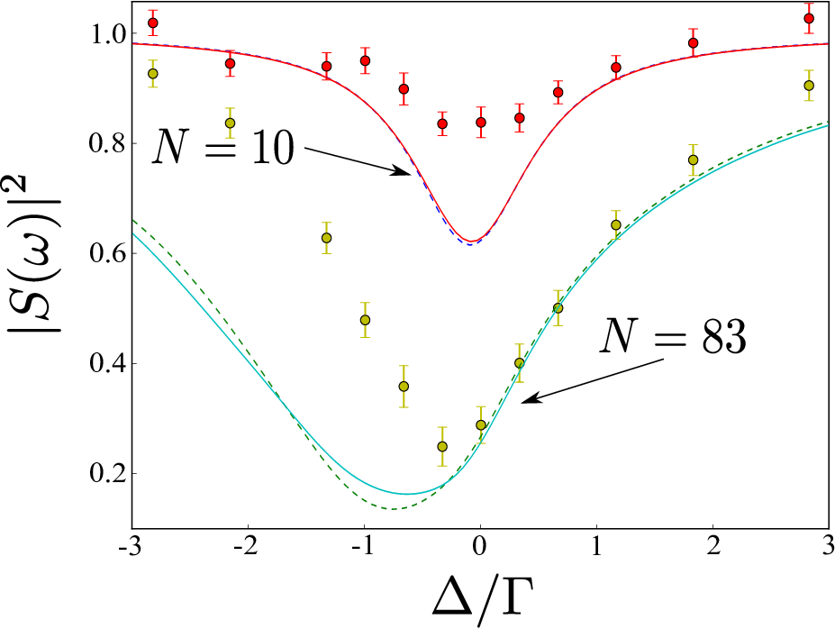
Reference [9] reports the coherent light transported through a cloud of atoms. They observe the transfer function:

which is essentially a quantification of the interference between the electric field from the laser, $\boldsymbol{E}_{l}$, and the electric field scattered off of the atoms, $\boldsymbol{E}_{s}$, at the position of the detector. In Fig. 6 we compare the results from both Eq. (II.2) and the calculations that keep the first-order correlations in Eq. (II.3). This simulation uses the experimental parameters given in Ref. [9]. The cloud now has a fixed size: $\sigma_{x}=1.5\lambda$, $\sigma_{y}=\sigma_{z}=0.25\lambda$, which for the clouds of $10$ and $83$ atoms shown, give values of $\lambda^{3}\mathcal{N}\simeq 2.4$ and $\lambda^{3}\mathcal{N}\simeq 19.9$ respectively. Unlike the previous simulations given above, the probe beam is now a linearly polarized Gaussian laser propagating in the $\hat{\boldsymbol{x}}$ direction, with an amplitude:

where $\frac{1}{q(x)}=\frac{1}{R(x)}+\frac{2i}{k{\rm w}^{2}(x)}$, $x_{R}=k{\rm w}^{2}/2$ is the Rayleigh length, ${\rm w}(x)={\rm w}\sqrt[\textbullet]{1+x^{2}/x_{R}^{2}}$, $E_{0}$ is the field amplitude, and $R(x)=x+x^{2}_{R}/x$. Where ${\rm w}=1.54\lambda$ is the waist of the laser. When comparing with the experimental data, one can see that the inclusion of correlations between Zeeman states does not explain the difference between the observations and the calculations. While, similar to experimental observations, the calculations that include Zeeman correlations have a significantly smaller redshift than the results obtained using Eq. (II.2), the calculated lineshape is still non-Lorentzian. This differs from experiment, where the key qualitative experimental observation is that the lineshape is Lorentzian [9]. This could indicate that the assumption of an initial, completely uncorrelated, mixture of Zeeman states is incorrect.

References

- [1] R. H. Dicke, Phys. Rev. 93, 99 (1954).
- [2] M.-T. Rouabah, M. Samoylova, R. Bachelard, P. W. Courteille, R. Kaiser, and N. Piovella, J. Opt. Soc. Am. A 31, 1031 (2014).
- [3] T. Bienaimé, N. Piovella, and R. Kaiser, Phys. Rev. Lett. 108, 123602 (2012).
- [4] W. Guerin, M. O. Araújo, and R. Kaiser, Phys. Rev. Lett. 116, 083601 (2016a).
- [5] S. Bromley, B. Zhu, M. Bishof, X. Zhang, T. Bothwell, Schachenmayer, N. J.T.L., R. Kaiser, S. F. Yelin, M. Lukin, A. Rey, and J. Ye, Nat. Commun. 7 (2016).
- [6] J. Pellegrino, R. Bourgain, S. Jennewein, Y. R. Sortais, A. Browaeys, S. Jenkins, and J. Ruostekoski, Phys. Rev. Lett. 113, 133602 (2014).
- [7] J. Javanainen, J. Ruostekoski, Y. Li, and S.-M. Yoo, Phys. Rev. Lett. 112, 113603 (2014).
- [8] G. Facchinetti, S. D. Jenkins, and J. Ruostekoski, Phys. Rev. Lett. 117, 243601 (2016).
- [9] S. Jennewein, M. Besbes, N. J. Schilder, S. D. Jenkins, C. Sauvan, J. Ruostekoski, J.-J. Greffet, Y. R. P. Sortais, and A. Browaeys, Phys. Rev. Lett. 116, 233601 (2016).
- [10] S. D. Jenkins, J. Ruostekoski, J. Javanainen, S. Jennewein, R. Bourgain, J. Pellegrino, Y. R. P. Sortais, and A. Browaeys, Phys. Rev. A 94, 023842 (2016).
- [11] M. D. Lee, S. D. Jenkins, and J. Ruostekoski, Physical Review A 93, 063803 (2016).
- [12] A. A. Svidzinsky, J.-T. Chang, and M. O. Scully, Phys. Rev. A 81, 053821 (2010).
- [13] H. Harde and D. Grischkowsky, JOSA B 8, 1642 (1991).
- [14] M. Gross and S. Haroche, Physics Reports 93, 301 (1982).
- [15] M. Gross, C. Fabre, P. Pillet, and S. Haroche, Physical Review Letters 36, 1035 (1976).
- [16] M. Gross, J. Raimond, and S. Haroche, Physical Review Letters 40, 1711 (1978).
- [17] N. E. Rehler and J. H. Eberly, Physical Review A 3, 1735 (1971).
- [18] R. T. Sutherland and F. Robicheaux, Phys. Rev. A 93, 023407 (2016a).
- [19] R. T. Sutherland and F. Robicheaux, Phys. Rev. A 94, 013847 (2016b).
- [20] R. T. Sutherland and F. Robicheaux, Phys. Rev. A 95, 033839 (2017).
- [21] R. J. Bettles, S. A. Gardiner, and C. S. Adams, Phys. Rev. A 92, 063822 (2015).
- [22] R. J. Bettles, S. A. Gardiner, and C. S. Adams, Phys. Rev. Lett. 116, 103602 (2016a).
- [23] M. O. Scully, E. S. Fry, C. H. R. Ooi, and K. Wódkiewicz, Phys. Rev. Lett. 96, 010501 (2006).
- [24] M. Scully, Laser Phys. 17, 635 (2007).
- [25] M. O. Scully, Phys. Rev. Lett. 102, 143601 (2009).
- [26] M. O. Scully, Phys. Rev. Lett. 115, 243602 (2015).
- [27] H. Bender, C. Stehle, S. Slama, R. Kaiser, N. Piovella, C. Zimmermann, and P. W. Courteille, Phys. Rev. A 82, 011404 (2010).
- [28] P. W. Courteille, S. Bux, E. Lucioni, K. Lauber, T. Bienaime, R. Kaiser, and N. Piovella, The Eur. Phys. J. D 58, 69 (2010).
- [29] W. Guerin, M. O. Araújo, and R. Kaiser, Phys. Rev. Lett. 116, 083601 (2016b).
- [30] H. H. Jen, M.-S. Chang, and Y.-C. Chen, Phys. Rev. A 94, 013803 (2016).
- [31] H. Jen, arXiv preprint arXiv:1706.00888 (2017).
- [32] T. Ido, T. H. Loftus, M. M. Boyd, A. D. Ludlow, K. W. Holman, and J. Ye, Phys. Rev. Lett. 94, 153001 (2005).
- [33] J. Ruostekoski and J. Javanainen, Phys. Rev. A 55, 513 (1997).
- [34] J. Hernández, L. Noordam, and F. Robicheaux, J. Phys. Chem. B 109, 15808 (2005).
- [35] A. S. Kuraptsev and I. M. Sokolov, Phys. Rev. A 90, 012511 (2014).
- [36] R. Monshouwer, M. Abrahamsson, F. van Mourik, and R. van Grondelle, The Journal of Physical Chemistry B 101, 7241 (1997).
- [37] M. A. Palacios, F. L. de Weerd, J. A. Ihalainen, R. van Grondelle, and H. van Amerongen, The Journal of Physical Chemistry B 106, 5782 (2002).
- [38] B. Zhu, J. Schachenmayer, M. Xu, F. Herrera, J. G. Restrepo, M. J. Holland, and A. M. Rey, New Journal of Physics 17, 083063 (2015).
- [39] B. Zhu, J. Cooper, J. Ye, and A. M. Rey, Physical Review A 94, 023612 (2016).
- [40] R. J. Bettles, S. A. Gardiner, and C. S. Adams, Phys. Rev. A 94, 043844 (2016b).
- [41] S. Roof, K. Kemp, M. Havey, and I. Sokolov, Physical Review Letters 117, 073003 (2016).
- [42] R. Kubo, Journal of the Physical Society of Japan 17, 1100 (1962), https://doi.org/10.1143/JPSJ.17.1100 .
- [43] D. Meiser, J. Ye, D. R. Carlson, and M. J. Holland, Phys. Rev. Lett. 102, 163601 (2009).
- [44] D. F. V. James, Phys. Rev. A 47, 1336 (1993).
- [45] G. S. Agarwal and A. K. Patnaik, Phys. Rev. A 63, 043805 (2001).
- [46] R. Shankar, Principles of quantum mechanics (Springer Science & Business Media, 2012).