Simulation of Fluid Particle Cutting - Validation and Case Study

For meshfree particle methods the interfaces between fluids are easily tracked by using flags on the particles. Initially, we assign different flags or color function $c$ of particles representing the corresponding fluids. We define the color function $c=1$ for fluid type 1 and $c=2$ for fluid type 2. On the interface and its vicinity, the Shepard interpolation is applied for smoothing of the color functions using

$$\tilde{c}({\bf x})=\frac{\sum_{i=1}^{m}w_{i}c_{i}}{\sum_{i=1}^{m}},$$

(5)

where $m$ is the number of neighbor of arbitrary particle having position ${\bf x}$, $c_{i}$ are the color values at neighboring particle $i$ and $w_{i}$ is the weight as a function of distance from ${\bf x}$ to $\bf{x}_{i}$ given by

$\displaystyle w_{i}=w({\bf x}_{i}-{\bf x};h)=\left\{\begin{array}[]{l}\exp(-\alpha\frac{\|{\bf x}_{i}-{\bf x}\|^{2}}{h^{2}}),\quad\mbox{if }\frac{\|{\bf x}_{i}-{\bf x}\|}{h}\leq 1\\ 0,\qquad\qquad\quad\quad\quad\quad\mbox{else},\end{array}\right.$

where $\alpha$ is a positive constant After smoothing the color function, we compute the unit normal vector

$${\bf n}=\frac{\nabla\tilde{c}}{|\nabla\tilde{c}|}.$$

(9)

Finally, we compute the curvature by

$$\kappa=-\nabla\cdot{\vec{n}}.$$

(10)

The quantity $\delta_{s}$ is approximated as

$$\delta_{s}\approx|\nabla\tilde{c}|.$$

(11)

Here, $\delta_{s}$ is non-zero in the vicinity of the interface and vanishes far from it.

We solve the Navier-Stokes equations (3) with the help of Chorin’s projection method [7]. Here, the projection method is adopted in the Lagrangian meshfree particle method. Consider the discrete time levels $t^{n}=n~dt,n=0,1,2,\ldots$ with time step $dt$. Let ${\bf x}^{n}$ be the position of a particle at time level $n$.

In the Lagrangian particle scheme we compute the new particle positions at the time level $(n+1)$ by

$${\bf x}^{n+1}={\bf x}^{n}+dt\;{\bf v}^{n}$$

(12)

and then use Chorin’s pressure projection scheme in new positions of particles. The pressure projection scheme is divided into two steps. The first step consists of computing the intermediate velocity $\bf{v}^{*}$ with neglecting the pressure term

$${\bf v}^{*}={\bf v}^{n}+\frac{dt}{\rho}\nabla\cdot(2\mu\tau^{*})+dt~{\bf g}+\frac{dt}{\rho}{\bf F}^{n}_{S}.$$

(13)

Since we use the Lagrangian formulation, we do not need to handle the nonlinear convective term. The second step consists of computation of pressure and the velocity at time level $(n+1)$ by solving the equation

$${\bf v}^{n+1}={\bf v}^{*}-dt\;\frac{\nabla p^{n+1}}{\rho}$$

(14)

where ${\bf v}^{n+1}$ should obey the continuity equation

$$\nabla\cdot{\bf v}^{n+1}=0.$$

(15)

We observe from the equation (14) that the new pressure $p^{n+1}$ is necessary in order to compute the new velocity. ${\bf v}^{n+1}$ . Now, we take the divergence of equation (14) on both sides and use of the continuity constraint (15), we obtain the pressure Poisson equation

$$\nabla\cdot\left(\frac{\nabla p^{n+1}}{\rho}\right)=\frac{\nabla\cdot{\bf v}^{*}}{dt}.$$

(16)

In order to derive the boundary condition for $p$ we project the equation (14) on the outward unit normal vector ${\bf n}$ at the boundary $\Gamma$ and then we obtain the Neumann boundary condition

$$\left(\frac{\partial p}{\partial{\bf n}}\right)^{n+1}=-\frac{\rho}{dt}({\bf v}^{n+1}_{\Gamma}-{\bf v}^{*}_{\Gamma})\cdot{\bf n},$$

(17)

where ${\bf v}_{\Gamma}$ is the value of ${\bf v}$ on $\Gamma$. Assuming ${\bf v}\cdot{\bf n}=0$ on $\Gamma$, we obtain

$$\left(\frac{\partial p}{\partial{\bf n}}\right)^{n+1}=0$$

(18)

on $\Gamma$.

We note that we have to approximate the spatial derivatives at each particle position as well as solve the second order elliptic problems for the velocities and the pressure. The spatial derivatives at each particle position are approximated from its neighboring clouds of particles based on the weighted least squares method. The weight is a function of a distance of a particle position to its neighbors. We observe that in Eq. 13 there is a discontinues coefficient $\mu$ inside the divergence operator since the viscosities of two liquid may have the ratio of up to 1 to 100. Similarly, the density ratio also has 1 to 1000, which can be seen also in Eq. 16. This discontinous coefficients have to be smoothed for stable computation. This is done using a similar procedure as for smoothing the color function. We denote the smoothed viscosity and density by $\tilde{\mu}$ and $\tilde{\rho}$, respectively. We note that we smooth the density and viscosity while solving Eqs. 13 and 16, but keep them constant on each phase of particles during the entire computational time. If the density and viscosity has larger ratios, we may have to iterate the smoothing 2 or 3 times. Finally, Eq. 13 and Eq. 16 can be re-expressed as

	$\displaystyle u^{*}-\frac{dt}{\tilde{\rho}}\nabla\tilde{\mu}\cdot\nabla u^{*}-dt\frac{\tilde{\mu}}{\tilde{\rho}}\Delta u^{*}$	$\displaystyle=$	$\displaystyle u^{n}+dt\;g_{x}+\frac{dt}{\rho}(\frac{\partial\tilde{\mu}}{\partial x}\frac{\partial u^{n}}{\partial x}+\frac{\partial\tilde{\mu}}{\partial y}\frac{\partial v^{n}}{\partial x})$		(19)
	$\displaystyle v^{*}-\frac{dt}{\tilde{\rho}}\nabla\tilde{\mu}\cdot\nabla v^{*}-dt\frac{\tilde{\mu}}{\tilde{\rho}}\Delta v^{*}$	$\displaystyle=$	$\displaystyle v^{n}+dt\;g_{y}+\frac{dt}{\tilde{\rho}}(\frac{\partial\tilde{\mu}}{\partial x}\frac{\partial u^{n}}{\partial y}+\frac{\partial\tilde{\mu}}{\partial y}\frac{\partial v^{n}}{\partial y})$		(20)
	$\displaystyle-\frac{\nabla\tilde{\rho}}{\tilde{\rho}}\cdot\nabla p^{n+1}+\Delta p^{n+1}$	$\displaystyle=$	$\displaystyle\tilde{\rho}\frac{\nabla\cdot{\vec{v}}^{*}}{dt}.$		(21)

Note that, for constant density, the first term of Eq. 21 vanishes and we get the pressure Poisson equation. Far from the interface we have $\tilde{\mu}=\mu$ and $\tilde{\rho}=\rho$. The momentum and pressure equations have the following general form

$$A\psi+{\bf B}\cdot\nabla\psi+C\Delta\psi=f,$$

(22)

where $A,{\bf B}$ and $C$ are known quantities. This equation is solved with Dirichlet or Neumann boundary conditions

$$\psi=\psi_{\Gamma D}\quad\quad\quad\mbox{or}\quad\frac{\partial\psi}{\partial\vec{n}}=\psi_{\Gamma N}.$$

(23)

Remark: For the x component of the momentum equations we have $A=1,{\bf B}=-\frac{dt}{\tilde{\rho}}\nabla\tilde{\mu},C=-\frac{dt}{\tilde{\rho}}\tilde{\mu}$ and $f$ is equal to the right hand side of Eq. 19. Similarly, for the pressure equation Eq. 21 we have $A=0,{\bf B}=\frac{\nabla\tilde{\rho}}{\tilde{\rho}},C=1$ and $f=\tilde{\rho}\frac{\nabla\cdot{\bf v}^{*}}{dt}$.

In the following section we describe the method of solving equations Eqs. 22 - 23 by a meshfree particle method, called the Finite Pointset Method (FPM).

In this subsection we describe a meshfree method for solving second order elliptic boundary value problems of type Eqs. 22 - 23. The method will be described in a two-dimensional space. The extension of the method to three-dimensional space is straightforward. Let $\Omega\in R^{2}$ be the computational domain. The domain $\Omega$ is approximated by particles of positions ${\bf x}_{i},i=1,\ldots,N$, which are socalled numerical grid points. Consider a scaler function $\psi({\bf x})$ and let $\psi_{i}=\psi({\bf x}_{i})$ be its discrete values at particle indices $i=1,\ldots,N$. We approximate the spatial derivatives of $\psi({\bf x})$ at an arbitrary position ${\bf x}\in\{{\bf x}_{i},i=1,\ldots,N\}$, from the values of its neighboring points. We introduce a weight function $w=w({\bf x}_{i}-{\bf x},h)$ with a compact support $h$. The value of $h$ can be $2.5$ to $3$ times the initial spacing of particles such that the minimum number of neighbor is guaranteed in order to approximate the spatial derivatives. But it is user defined quantity. This weight function has two properties, first, it avoids the influence of the far particles and the second it reduce the unnecessary neighbors in the computational part. One can consider different weight function, in this paper we consider the Gaussian weight function defined in (5.1), where $\alpha$ is equal to $6.25$. Let $P({\bf x},h)=\{{\bf x}_{j}:j=1,2,\ldots,m\}$ be the set of $m$ neighboring particles of ${\bf x}$ in a circle of radius $h$. We note that the point ${\bf x}$ is itself one of ${\bf x}_{j}$.

We consider Taylor expansions of $\psi({\bf x}_{i})$ around ${\bf x}=(x,y)$

	$\displaystyle\psi(x_{j},y_{j})=\psi(x,y)+\frac{\partial\psi}{\partial x}(x_{j}-x)+\frac{\partial\psi}{\partial y}(y_{j}-y)+\frac{1}{2}\frac{\partial^{2}\psi}{\partial x^{2}}(x_{j}-x)^{2}+$
	$\displaystyle\quad\quad\quad\frac{\partial^{2}\psi}{\partial x\partial y}(x_{j}-x)(y_{j}-y)+\frac{1}{2}\frac{\partial^{2}\psi}{\partial y^{2}}(y_{j}-y)^{2}+e_{j}$		(24)

for $j=1,\ldots,m$, where $e_{j}$ is the residual error. Let the coefficients of the Taylor expansion be denoted by

$a_{1}=\psi(x,y),\;a_{2}=\frac{\partial\psi}{\partial x},\;a_{3}=\frac{\partial\psi}{\partial y},\;$

$a_{4}=\frac{\partial^{2}\psi}{\partial x^{2}},\;a_{5}=\frac{\partial^{2}\psi}{\partial x\partial y},a_{6}=\frac{\partial^{2}\psi}{\partial y^{2}}.\;$

We add the constraint that at particle position $(x,y)$ the partial differential equation (22) should be satisfied. If the point $(x,y)$ lies on the boundary, also the boundary condition (23) needs to be satisfied. Therefore, we add Eqs. 22 and 23 to the $m$ equations (24). Equations 22 and 23 are re-expressed as

	$\displaystyle Aa_{1}+B_{1}a_{2}+B_{2}a_{3}+C(a_{4}+a_{6})=f+e_{m+1}$		(25)
	$\displaystyle n_{x}a_{2}+n_{y}a_{3}=\psi_{\Gamma N}+e_{m+2},$		(26)

where ${\bf B}=(B_{1},B_{2})$ and $n_{x},n_{y}$ are the $x,y$ components of the unit normal vector ${\bf n}$ on the boundary $\Gamma$. The coefficients $a_{i},i=1,\ldots,6$ are the unknowns.

We have six unknowns and $m+1$ equations for the interior points and $m+2$ unknowns for the Neumann boundary points. This means, we always need a minimum of six neighbors. In general, we have more than six neighbors, so the system is overdetermined and can be written in matrix form as

$${\bf e}=M{\bf a}-{\bf b},$$

(27)

where

$\displaystyle M=\left(\begin{array}[]{cccccc}1&~dx_{1}&~dy_{1}&~\frac{1}{2}dx^{2}_{1}&~dx_{1}dy_{1}&~\frac{1}{2}dy^{2}_{1}\\ \vdots&\vdots&\vdots&\vdots&\vdots&\vdots\\ 1&~dx_{m}&~dy_{m}&~\frac{1}{2}dx^{2}_{m}&~dx_{m}dy_{m}&~\frac{1}{2}dy^{2}_{m}\\ A&~B_{1}&~B_{2}&~C&~0&~C\\ 0&~n_{x}&~n_{y}&~0&~0&~0\end{array}\right),$

with the vectors given by ${\bf a}=\left(a_{1},a_{2},\ldots a_{6}\right)^{T},\;{\bf b}=\left(\psi_{1},\ldots,\psi_{m},f,\psi_{N}\right)^{T}$ and ${\bf e}=\left(e_{1},\ldots,e_{m},e_{m+1},e_{m+2}\right)^{T}$ and $dx_{j}=x_{j}-x,\;dy_{j}=y_{j}-y$. For the numerical implementation, we set $n_{x}=n_{y}=0$ and $\psi_{\Gamma N}=0$ for the interior particles. For the Dirichlet boundary particles, we directly prescribe the boundary conditions, and for the Neumann boundary particles the matrix coefficients are given by Eq. 5.3. The unknowns $a_{i}$ are computed by minimizing a weighted error over the neighboring points. Thus, we have to minimize the following quadratic form

$$J=\sum_{i=1}^{m+2}w_{i}e_{i}^{2}=(M{\bf a}-{\bf b})^{T}W(M{\bf a}-{\bf b}),$$

(34)

where

$\displaystyle W=\left(\begin{array}[]{cccccc}w_{1}&0&\cdots&0&0&0\\ \vdots&\vdots&\cdots&\vdots\\ 0&0&\cdots&w_{m}&0&0\\ 0&0&\cdots&0&1&0\\ 0&0&\cdots&0&0&1\end{array}\right).$

The minimization of $J$ with respect to ${\bf a}$ formally yields ( if $M^{T}WM$ is nonsingular)

$${\bf a}=(M^{T}WM)^{-1}(M^{T}W){\bf b}.$$

(36)

In Eq. 36 the vector $(M^{T}W){\bf b}$ is explicitly given by

	$\displaystyle(M^{T}W){\bf b}=\left(\sum_{j=1}^{m}w_{j}\psi_{j},\;\sum_{j=1}^{m}w_{j}dx_{j}\psi_{j}+B_{1}f+n_{x}\psi_{\Gamma N},\right.$
	$\displaystyle\left.\sum_{j=1}^{m}w_{j}dy_{j}\psi_{j}+B_{2}f+n_{y}\psi_{\Gamma N},\;\frac{1}{2}\sum_{j=1}^{m}w_{j}dx^{2}_{j}\psi_{j}+Cf,\;\right.$
	$\displaystyle\left.\sum_{j=1}^{m}w_{j}dx_{j}dy_{j}\psi_{j},\;\frac{1}{2}\sum_{j=1}^{m}w_{j}dy^{2}_{j}\psi_{j}+Cf\;\right)^{T}.$		(37)

Equating the first components on both sides of Eq. 36, we get

	$\displaystyle\psi=Q_{1}\left(\sum_{j=1}^{m}w_{j}\psi_{j}\right)+Q_{2}\left(\sum_{j=1}^{m}w_{j}dx_{j}\psi_{j}+B_{1}f+n_{x}\psi_{\Gamma N}\right)+$
	$\displaystyle Q_{3}\left(\sum_{j=1}^{m}w_{j}dy_{j}\psi_{j}+B_{2}f+n_{y}\psi_{\Gamma N}\right)+Q_{4}\left(\frac{1}{2}\sum_{j=1}^{m}w_{j}dx^{2}_{j}\psi_{j}+Cf\right)+$
	$\displaystyle Q_{5}\left(\sum_{j=1}^{m}w_{j}dx_{j}dy_{j}\psi_{j}\right)+Q_{6}\left(\frac{1}{2}\sum_{j=1}^{m}w_{j}dy^{2}_{j}\psi_{j}+Cf\right),$		(38)

where $Q_{1},Q_{2},\ldots,Q_{6}$ are the components of the first row of the matrix $(M^{T}WM)^{-1}$. Rearranging the terms, we have

	$\displaystyle\psi-\sum_{j=1}^{m}w_{j}\left(Q_{1}+Q_{2}dx_{j}+Q_{3}dy_{j}+Q_{4}\frac{dx^{2}_{j}}{2}+Q_{5}dx_{j}~dy_{j}+Q_{6}\frac{dy^{2}_{j}}{2}\right)\psi_{j}=$
	$\displaystyle\left(Q_{2}B_{1}+Q_{3}B_{2}+Q_{4}C+Q_{6}C\right)f+\left(Q_{2}n_{x}+Q_{3}n_{y}\right)\psi_{\Gamma N}.\quad\quad\quad$		(39)

We obtain the following sparse linear system of equations for the unknowns $\psi_{i},i=1,\ldots,N$

	$\displaystyle\psi_{i}-\sum_{j=1}^{m(i)}w_{i_{j}}\left(Q_{1}+Q_{2}dx_{i_{j}}+Q_{3}dy_{i_{j}}+Q_{4}\frac{dx^{2}_{i_{j}}}{2}+Q_{5}dx_{i_{j}}dy_{i_{j}}+Q_{6}\frac{dy^{2}_{i_{j}}}{2}\right)\psi_{i_{j}}=$
	$\displaystyle\left(Q_{2}B_{1}+Q_{3}B_{2}+Q_{4}C+Q_{6}C\right)f_{i}+\left(Q_{2}n_{x}+Q_{3}n_{y}\right)\psi_{\Gamma N_{i}}.\quad\quad\quad$		(40)

In matrix form we have

$$L{\bf\Psi}={\bf R},$$

(41)

where ${\bf R}$ is the right-hand side vector, ${\bf\Psi}$ is the unknown vector and $L$ is the sparse matrix having non-zero entries only for neighboring particles.

We solve the sparse system (41) by the Gauss-Seidel method. In each time iteration the initial values of $\psi$ for time step $n+1$ are taken as the values from previous time step $n$. While solving the equations for intermediate velocities and the pressure will require more iterations in the first few time steps. After a certain number of time steps, the velocities values and the pressure values at the old time step are close to those of new time step, so the number of iterations is dramatically reduced.

We stop the iteration process if

$$\frac{\sum_{i=1}^{N}|\psi_{i}^{\tau+1}-\psi_{i}^{(\tau)}|}{\sum_{i=1}^{N}|\psi^{(\tau+1)}_{i}|}<\epsilon,$$

(42)

for $\tau=0,1,2,\ldots$ and $\epsilon$ is a small positive constant and can be defined by the user.

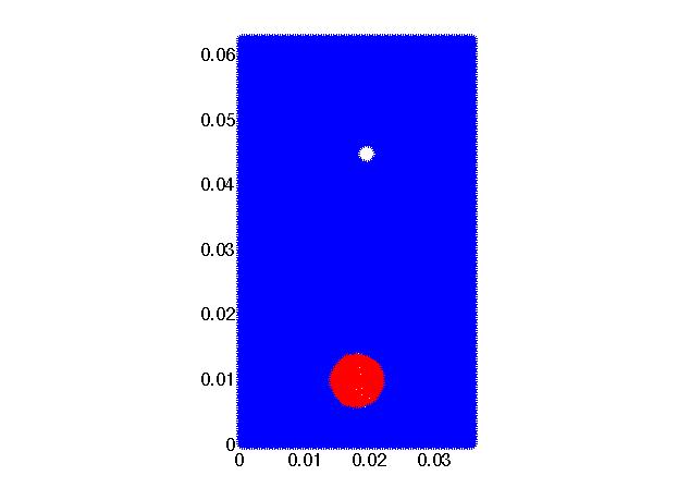
In a first step, we validate the simulations with the experimental results of the single bubble cutting in reversed osmosis purified water. We apply the same bubble diameter from the experiments ($6.5mm$) and the wire diameter of $3mm$ in the simulation. The viscosity of the fluid (water) is $\mu_{l}=0.001Pa.s$ and the interfacial tension between water and air is $\sigma=0.072N/m$.. The density of water is $\rho_{l}=998.2kg/m^{3}$ and the density of air is approximated by $\rho_{g}=1kg/m^{3}$ and the dynamic viscosity of air is $\mu_{g}=2e^{-5}$. . For the numerical simulations we consider a two-dimensional geometry of size $36mm\times 63mm$. The initial bubble position has the center at $x=18mm$ and $y=10mm$ and the wire has the center at $x=19.5mm$ and $y=45mm$ as shown in Fig. 3. The bubble is approximated by red particles, the liquid is approximated by blue particles. The white circular spot is the position of the wire. We have considered the total number of boundary particles, (including 4 walls and the wire) equal to $527$ and the initial number of interior particles equal to $18310$. The constant time step $t=5e^{-6}$ is considered. Here the horizontal distance between the initial center of bubble and the wire is $d_{x}=1.5mm$. In all four walls and the wire we have considered no-slip boundary conditions. Initially, the velocity and pressure are equal to zero. The gravitational force is ${\bf g}=(0,-9.81)m/s^{2}$.

The comparison between simulation and experiment is depicted in Fig. 4 and 5. We extracted a time sequence from the experiments and the corresponding simulations, starting at 0.19 seconds simulated time to 0.27 seconds. The temporal distance between each image is 0.02 s. The rising bubble approaches the wire and starts to deform. There is no direct contact during this phase between the bubble and the wire. Due to the non central approach to the wire, the bubble is cut in a smaller daughter bubble (right) and a larger bubble (left). The larger bubble has three times the diameter of the smaller bubble. The comparison of the cutting process gives a qualitatively good agreement between the experiment and the simulation. Also the shape and size of the mother and daughter bubbles are qualitatively very good agreement. A detailed comparison of the bubble path from experiment and simulation is shown in Fig. 6. The bubble position during first contact is important, which agrees well between experiment and simulation. Nevertheless, the path of the larger bubble in the simulation shows after the cutting a slightly different behaviour than in the experiment. In the experiment, the larger bubble moves inwards again, while the bubble in the simulation moves horizontally away from the wire, which may arise from a slight horizontally movement of the bubble in the experiment. The cutting of the bubble also depends on the bubble velocity, plotted in Fig. 7. The bubble accelerates in the simulation and finally reaches the same end velocity that is observed in the experiment. After the splitting into two daughter bubbles, the larger daughter bubble raises faster than the smaller one. The experimental results are governed by higher fluctuations especially for the smaller bubble, which results from very short temporal distances between the images and fluctuations by detecting the bubble interface. Neverthless, the average velocity for the smaller bubble fits with 0.12 m/s quiet well to the simulated result.

The computational domain is the same as in the previous section. However, the position of the wire is changed. The data has been taken from chapter 6 of [6]. The liquid has density $\rho_{l}=1250kg/m^{3}$, dynamical viscosity $\mu_{l}=0.219Pa.s$. Similarly the gas density $\rho_{g}=1kg/m^{3}$ and the viscosity $\mu_{g}=2e^{-5}Pa.s$. The surface tension coefficient $\sigma=0.0658N/m$. We consider a bubble of diameter $9.14mm$ with its initial center at $(18mm,9mm)$. We consider a wire (in 2D a circle) of diameter $3.1mm$ with different centers at $y=45mm$ and $x=18mm,18.5mm,19mm$ and $19.5mm$. This means, we consider the initial distance $d_{x}$ between the center of the bubble and the center of the wire equal to $d_{x}=0mm,0.5mm,1mm,1.5mm$. Fig. 8 shows the initial geometry with $d_{x}=0mm$. The initial number of particles and the time step are the same as in the low viscosity case. The initial and boundary conditions and the rest of other parameters are same as in the previous case.

In Figs. 9 - 12 we have plotted the positions of the bubble and the wire for $d_{x}=0mm,0.5mm,1mm$ and $1.5mm$ at time $t=0.288,0.320,0.352$ and $t=0.384$ seconds, respectively. For $d_{x}=0$ we observe the wire located in the middle of the bubble as expected. When we increased the distance $d_{x}$ from $0.5mm$ to $1.5mm$, we observed that the left part of the bubble is increasing and the right part becomes smaller. We clearly observe that the daughter bubbles are symmetric for $d_{x}=0mm$ in contrast to the other cases. We further observe a small layer between the wire and the bubble. After $t=0.352$ seconds we observe the cutting of the bubble, see Figs. 11 and 12. Two daughter bubbles arise, a larger one on the left and a smaller one on the right side of the wire. The overall numerical results are comparable with the results presented in [6].

In Fig. 13 we have plotted the trajectories of the mother and bubble droplets. We observed that the mother droplet is cutted into two daughter bubble slightly below the wire, compare with Fig. 11. The trajectories are plotted up to time $t=0.5s$. We see that when the size of the daughter bubble is increasing, it travels longer than the smaller bubbles. The reason is that the rising velocity of the larger bubble is larger than the smaller ones, see Fig. 14 for the velocities of mother and daughter bubbles.

References

- [1] R. F. Mudde, and T. Saito Hydrodynamical similarities between bubble column and bubbly pipe flow, J. Fluid Mech. 437, 203–228, 2001.
- [2] F. Shakir Ahmed, B. A. Sensenich , S. A. Gheni , D. Znerdstrovic, and M. H. Al Dahhan textitBubble Dynamics in 2D Bubble Column: Comparison between High-Speed Camera Imaging Analysis and 4-Point Optical Probe, Chemical Engineering Communications 202, 85-95, 2014.
- [3] K. H. Choi, and W. K. Lee Comparison of Probe Methods for Measurement of Bubble Properties, Chemical Engineering Communications 91, 35-47, 1990.
- [4] H.-M.Prasser, D.Scholz, and C.Zippe Bubble size measurement using wire-mesh sensors, Flow Measurement and Instrumentation 12, 299-312, 2001.
- [5] H.-J. Bart, M. Mickler, H.B. Jildeh Optical Image Analysis and Determination of Dispersed Multi Phase Flow for Simulation and Control, In: Optical Imaging: Technology, Methods & Applications, Akira Tanaka and Botan Nakamura (eds.), 1-63, Nova Science, N.Y. Lancaster, 2012.
- [6] M. W. Baltussen, Bubbles on the cutting edge : direct numerical simulations of gas-liquid-solid three-phase flows, Preprint, TU Eindhoven, 2015.
- [7] A. Chorin, Numerical solution of the Navier-Stokes equations, Math. Comput. vol. 22 (1968) 745-762.
- [8] J.U. Brackbill, D.B. Kothe, C. Zemach, A continuum method for modeling surface tension, J. Comput. Phys. 100, 354�355, 1992.
- [9] J. P. Morris, Simulating Surface Tension with Smoothed Particle Hydrodynamics, Int. J. Numer. Methods Fluids, 33 (2000) 333-353.
- [10] C. Drumm, S. Tiwari, J. Kuhnert, H.-J. Bart, Finite pointset method for simulation of the liquid�liquid flow field in an extractor, Comput. Chem. Eng., 32, 2946, 2008.
- [11] S. Tiwari, A. Klar, S. Hardt, Numerical simulation of wetting phenomena by a meshfree particle method, J. Comput. Appl. Maths., 292(216), 469-485.
- [12] S. Tiwari, and J. Kuhnert, Finite pointset method based on the projection method for simulations of the incompressible Navier-Stokes equations, Meshfree Methods for Partial Differential Equations, eds. M. Griebel and M.A. Schweitzer, Lecture Notes in Computational Science and Engineering, Vol. 26 (Springer-Verlag, 2003), pp. 373-387.
- [13] S. Tiwari, and J. Kuhnert, Modelling of two-phase flow with surface tension by finite pointset method(FPM), J. Comp. Appl. Math, 203 (2007), pp. 376-386.