Deep Learning Techniques for Music Generation
– A Survey
Jean-Pierre Briot∗,11
1
Also
Visiting Professor at UNIRIO (Universidade Federal do Estado do Rio de Janeiro)
and Permanent Visiting Professor at PUC-Rio (Pontifícia Universidade Católica do Rio de Janeiro),
Rio de Janeiro, Brazil.,
Gaëtan Hadjeres†
and François-David Pachet‡
∗ Sorbonne Université, CNRS,
LIP6, F-75005 Paris, France
† Sony Computer Science Laboratories, CSL-Paris, F-75005 Paris, France
‡ Spotify Creator Technology Research Lab, CTRL, F-75008 Paris, France
This paper is a survey and an analysis of different ways of using deep learning (deep artificial neural networks) to generate musical content. We propose a methodology based on five dimensions for our analysis:
- •
Objective
- –
What musical content is to be generated?
Examples are: melody, polyphony, accompaniment or counterpoint.
- –
For what destination and for what use?
To be performed by a human(s) (in the case of a musical score), or by a machine (in the case of an audio file).
- –
- •
Representation
- –
What are the concepts to be manipulated?
Examples are: waveform, spectrogram, note, chord, meter and beat.
- –
What format is to be used?
Examples are: MIDI, piano roll or text.
- –
How will the representation be encoded?
Examples are: scalar, one-hot or many-hot.
- –
- •
Architecture
- –
What type(s) of deep neural network is (are) to be used?
Examples are: feedforward network, recurrent network, autoencoder or generative adversarial networks.
- –
- •
Challenge
- –
What are the limitations and open challenges?
Examples are: variability, interactivity and creativity.
- –
- •
Strategy
- –
How do we model and control the process of generation?
Examples are: single-step feedforward, iterative feedforward, sampling or input manipulation.
- –
For each dimension, we conduct a comparative analysis of various models and techniques and we propose some tentative multidimensional typology. This typology is bottom-up, based on the analysis of many existing deep-learning based systems for music generation selected from the relevant literature. These systems are described and are used to exemplify the various choices of objective, representation, architecture, challenge and strategy. The last section includes some discussion and some prospects.
Supplementary material is provided at the following companion web site:
www.briot.info/dlt4mg/
This paper is a simplified (weak DRM22 2 In addition to including high quality color figures, the book includes: a table of contents, a list of tables, a list of figures, a table of acronyms, a glossary and an index.) version of the following book [15]: Jean-Pierre Briot, Gaëtan Hadjeres and François-David Pachet, Deep Learning Techniques for Music Generation, Computational Synthesis and Creative Systems, Springer, 2019. Hardcover ISBN: 978-3-319-70162-2. eBook ISBN: 978-3-319-70163-9. Series ISSN: 2509-6575.
Chapter \thechapter Introduction
Deep learning has recently become a fast growing domain and is now used routinely for classification and prediction tasks, such as image recognition, voice recognition or translation. It became popular in 2012, when a deep learning architecture significantly outperformed standard techniques relying on handcrafted features in an image classification competition, see more details in Section id1.
We may explain this success and reemergence of artificial neural network techniques by the combination of:
- •
availability of massive data;
- •
availability of efficient and affordable computing power33 3 Notably, thanks to graphics processing units (GPU), initially designed for video games, which have now one of their biggest markets in data science and deep learning applications.;
- •
technical advances, such as:
There is no consensual definition for deep learning. It is a repertoire of machine learning (ML) techniques, based on artificial neural networks. The key aspect and common ground is the term deep. This means that there are multiple layers processing multiple hierarchical levels of abstractions, which are automatically extracted from data55 5 That said, although deep learning will automatically extract significant features from the data, manual choices of input representation, e.g., spectrum vs raw wave signal for audio, may be very significant for the accuracy of the learning and for the quality of the generated content, see Section 14.3.. Thus a deep architecture can manage and decompose complex representations in terms of simpler representations. The technical foundation is mostly artificial neural networks, as we will see in Chapter id1, with many extensions, such as: convolutional networks, recurrent networks, autoencoders, and restricted Boltzmann machines. For more information about the history and various facets of deep learning, see, e.g., a recent comprehensive book on the domain [63].
Driving applications of deep learning are traditional machine learning tasks66 6 Tasks in machine learning are types of problems and may also be described in terms of how the machine learning system should process an example (63, Section 5.1.1). Examples are: classification, regression and anomaly detection.: classification (for instance, identification of images) and prediction77 7 As a testimony of the initial DNA of neural networks: linear regression and logistic regression, see Section 18. (for instance, of the weather) and also more recent ones such as translation.
But a growing area of application of deep learning techniques is the generation of content. Content can be of various kinds: images, text and music, the latter being the focus of our analysis. The motivation is in using now widely available various corpora to automatically learn musical styles and to generate new musical content based on this.
1 Motivation
1.1 Computer-Based Music Systems
The first music generated by computer appeared in 1957. It was a 17 seconds long melody named ‘‘The Silver Scale’’ by its author Newman Guttman and was generated by a software for sound synthesis named Music I, developed by Mathews at Bell Laboratories. The same year, ‘‘The Illiac Suite” was the first score composed by a computer [78]. It was named after the ILLIAC I computer at the University of Illinois at Urbana-Champaign (UIUC) in the United States. The human ‘‘meta-composers’’ were Lejaren A. Hiller and Leonard M. Isaacson, both musicians and scientists. It was an early example of algorithmic composition, making use of stochastic models (Markov chains) for generation as well as rules to filter generated material according to desired properties.
In the domain of sound synthesis, a landmark was the release in 1983 by Yamaha of the DX 7 synthesizer, building on groundwork by Chowning on a model of synthesis based on frequency modulation (FM). The same year, the MIDI88 8 Musical instrument digital interface, to be introduced in Section 12.1. interface was launched, as a way to interoperate various software and instruments (including the Yamaha DX 7 synthesizer). Another landmark was the development by Puckette at IRCAM of the Max/MSP real-time interactive processing environment, used for real-time synthesis and for interactive performances.
Regarding algorithmic composition, in the early 1960s Iannis Xenakis explored the idea of stochastic composition99 9 One of the first documented case of stochastic music, long before computers, is the Musikalisches Wurfelspiel (Dice Music), attributed to Wolfgang Amadeus Mozart. It was designed for using dice to generate music by concatenating randomly selected predefined music segments composed in a given style (Austrian waltz in a given key). [209], in his composition named ‘‘Atrées’’ in 1962. The idea involved using computer fast computations to calculate various possibilities from a set of probabilities designed by the composer in order to generate samples of musical pieces to be selected. In another approach following the initial direction of ‘‘The Illiac Suite’’, grammars and rules were used to specify the style of a given corpus or more generally tonal music theory. An example is the generation in the 1980s by Ebcioğlu’s composition software named CHORAL of a four-part chorale in the style of Johann Sebastian Bach, according to over 350 handcrafted rules [42]. In the late 1980s David Cope’s system named Experiments in Musical Intelligence (EMI) extended that approach with the capacity to learn from a corpus of scores of a composer to create its own grammar and database of rules [27].
Since then, computer music has continued developing for the general public, if we consider, for instance, the GarageBand music composition and production application for Apple platforms (computers, tablets and cellphones), as an offspring of the initial Cubase sequencer software, released by Steinberg in 1989.
1.2 Autonomy versus Assistance
When talking about computer-based music generation, there is actually some ambiguity about whether the objective is
- •
to design and construct autonomous music-making systems – two recent examples being the deep-learning based Amper™ and Jukedeck systems/companies aimed at the creation of original music for commercials and documentary; or
- •
The quest for autonomous music-making systems may be an interesting perspective for exploring the process of composition1010 10 As Richard Feynman coined it: “What I cannot create, I do not understand.” and it also serves as an evaluation method. An example of a musical Turing test1111 11 Initially codified in 1950 by Alan Turing and named by him the “imitation game” [191], the ‘‘Turing test’’ is a test of the ability for a machine to exhibit intelligent behavior equivalent to (and more precisely, indistinguishable from) the behavior of a human. In his imaginary experimental setting, Turing proposed the test to be a natural language conversation between a human (the evaluator) and a hidden actor (another human or a machine). If the evaluator cannot reliably tell the machine from the human, the machine is said to have passed the test. will be introduced in Section 44.2. It consists in presenting to various members of the public (from beginners to experts) chorales composed by J. S. Bach or generated by a deep learning system and played by human musicians1212 12 This is to avoid the bias (synthetic flavor) of a computer rendered generated music.. As we will see in the following, deep learning techniques turn out to be very efficient at succeeding in such tests, due to their capacity to learn musical style from a given corpus and to generate new music that fits into this style. That said, we consider that such a test is more a means than an end.
A broader perspective is in assisting human musicians during the various steps of music creation: composition, arranging, orchestration, production, etc. Indeed, to compose or to improvise1313 13 Improvisation is a form of real time composition., a musician rarely creates new music from scratch. S/he reuses and adapts, consciously or unconsciously, features from various music that s/he already knows or has heard, while following some principles and guidelines, such as theories about harmony and scales. A computer-based musician assistant may act during different stages of the composition, to initiate, suggest, provoke and/or complement the inspiration of the human composer.
That said, as we will see, the majority of current deep-learning based systems for generating music are still focused on autonomous generation, although more and more systems are addressing the issue of human-level control and interaction.
1.3 Symbolic versus Sub-Symbolic AI
Artificial Intelligence (AI) is often divided into two main streams1414 14 With some precaution, as this division is not that strict.:
- •
symbolic AI – dealing with high-level symbolic representations (e.g., chords, harmony…) and processes (harmonization, analysis…); and
- •
sub-symbolic AI – dealing with low-level representations (e.g., sound, timbre…) and processes (pitch recognition, classification…).
Examples of symbolic models used for music are rule-based systems or grammars to represent harmony. Examples of sub-symbolic models used for music are machine learning algorithms for automatically learning musical styles from a corpus of musical pieces. These models can then be used in a generative and interactive manner, to help musicians in creating new music, by taking advantage of this added “intelligent” memory (associative, inductive and generative) to suggest proposals, sketches, extrapolations, mappings, etc. This is now feasible because of the growing availability of music in various forms, e.g., sound, scores and MIDI files, which can be automatically processed by computers.
A recent example of an integrated music composition environment is FlowComposer [153], which we will introduce in Section 41.4. It offers various symbolic and sub-symbolic techniques, e.g., Markov chains for modeling style, a constraint solving module for expressing constraints, a rule-based module to produce harmonic analysis; and an audio mapping module to produce rendering. Another example of an integrated music composition environment is OpenMusic [3].
However, a deeper integration of sub-symbolic techniques, such as deep learning, with symbolic techniques, such as constraints and reasoning, is still an open issue1515 15 The general objective of integrating sub-symbolic and symbolic levels into a complete AI system is among the “Holy Grails” of AI., although some partial integrations in restricted contexts already exist (see, for example, Markov constraints in [149, 7] and an example of use for FlowComposer in Section 41.4).
1.4 Deep Learning
The motivation for using deep learning (and more generally machine learning techniques) to generate musical content is its generality. As opposed to handcrafted models, such as grammar-based [177] or rule-based music generation systems [42], a machine learning-based generation system can be agnostic, as it learns a model from an arbitrary corpus of music. As a result, the same system may be used for various musical genres.
Therefore, as more large scale musical datasets are made available, a machine learning-based generation system will be able to automatically learn a musical style from a corpus and to generate new musical content. As stated by Fiebrink and Caramiaux [52], some benefits are
- •
it can make creation feasible when the desired application is too complex to be described by analytical formulations or manual brute force design, and
- •
learning algorithms are often less brittle than manually designed rule sets and learned rules are more likely to generalize accurately to new contexts in which inputs may change.
Moreover, as opposed to structured representations like rules and grammars, deep learning is good at processing raw unstructured data, from which its hierarchy of layers will extract higher level representations adapted to the task.
1.5 Present and Future
As we will see, the research domain in deep learning-based music generation has turned hot recently, building on initial work using artificial neural networks to generate music (e.g., the pioneering experiments by Todd in 1989 [190] and the CONCERT system developed by Mozer in 1994 [139]), while creating an active stream of new ideas and challenges made possible thanks to the progress of deep learning. Let us also note the growing interest by some private big actors of digital media in the computer-aided generation of artistic content, with the creation by Google in June 2016 of the Magenta research project [48] and the creation by Spotify in September 2017 of the Creator Technology Research Lab (CTRL) [176]. This is likely to contribute to blurring the line between music creation and music consumption through the personalization of musical content [2].
2 This Book
The lack (to our knowledge) of a comprehensive survey and analysis of this active research domain motivated the writing of this book, built in a bottom-up way from the analysis of numerous recent research works. The objective is to provide a comprehensive description of the issues and techniques for using deep learning to generate music, illustrated through the analysis of various architectures, systems and experiments presented in the literature. We also propose a conceptual framework and typology aimed at a better understanding of the design decisions for current as well as future systems.
2.1 Other Books and Sources
To our knowledge, there are only a few partial attempts at analyzing the use of deep learning for generating music. In [14], a very preliminary version of this work, Briot et al. proposed a first survey of various systems through a multicriteria analysis (considering as dimensions the objective, representation, architecture and strategy). We have extended and consolidated this study by integrating as an additional dimension the challenge (after having analyzed it in [16]).
In [65], Graves presented an analysis focusing on recurrent neural networks and text generation. In [90], Humphrey et al. presented another analysis, sharing some issues about music representation (see Section id1) but dedicated to music information retrieval (MIR) tasks, such as chord recognition, genre recognition and mood estimation. On MIR applications of deep learning, see also the recent tutorial paper by Choi et al. [21].
One could also consult the proceedings of some recently created international workshops on the topic, such as
For a more general survey of computer-based techniques to generate music, the reader can refer to general books such as
About machine learning in general, some examples of textbooks are
2.2 Other Models
We have to remember that there are various other models and techniques for using computers to generate music, such as rules, grammars, automata, Markov models and graphical models. These models are either manually defined by experts or are automatically learnt from examples by using various machine learning techniques. They will not be addressed in this book as we are concerned here with deep learning techniques. However, in the following section we make a quick comparison of deep learning and Markov models.
2.3 Deep Learning versus Markov Models
Deep learning models are not the only models able to learn musical style from examples. Markov chain models are also widely used, see, for example, [146]. A quick comparison (inspired by the analysis of Mozer in [139]1616 16 Note that he made his analysis in in 1994, long before the deep learning wave.) of the pros (+) and cons (–) of deep neural network models and Markov chain models is as follows:
- +
-
Markov models are conceptually simple.
- +
-
Markov models have a simple implementation and a simple learning algorithm, as the model is a transition probability table1717 17 Statistics are collected from the dataset of examples in order to compute the probabilities..
- –
-
Neural network models are conceptually simple but the optimized implementations of current deep network architectures may be complex and need a lot of tuning.
- –
-
Order 1 Markov models (that is, considering only the previous state) do not capture long-term temporal structures.
- –
-
Order n Markov models (considering n previous states) are possible but require an explosive training set size1818 18 See the discussion in (139, page 249). and can lead to plagiarism1919 19 By recopying too long sequences from the corpus. Some promising solution is to consider a variable order Markov model and to constrain the generation (through min order and max order constraints) on some sweet spot between junk and plagiarism [152]..
- +
-
Neural networks can capture various types of relations, contexts and regularities.
- +
-
Deep networks can learn long-term and high-order dependencies.
- +
-
Markov models can learn from a few examples.
- –
-
Neural networks need a lot of examples in order to be able to learn well.
- –
-
Markov models do not generalize very well.
- +
-
Neural networks generalize better through the use of distributed representations [82].
- +
- –
-
Deep networks are generative models with a distributed representation and therefore with no direct control to be attached2121 21 This issue as well as some possible solutions will be discussed in Section 40.1..
As deep learning implementations are now mature and a large number of examples are available, deep learning-based models are in high demand for their characteristics. That said, other models (such as Markov chains, graphical models, etc.) are still useful and used and the choice of a model and its tuning depends on the characteristics of the problem.
2.4 Requisites and Roadmap
This book does not require prior knowledge about deep learning and neural networks nor music.
Chapter id1 Introduction (this chapter) introduces the purpose and rationale of the book.
Chapter id1 Method introduces the method of analysis (conceptual framework) and the five dimensions at its basis (objective, representation, architecture, challenge and strategy), dimensions that we discuss within the next four chapters.
Chapter id1 Objective concerns the different types of musical content that we want to generate (such as a melody or an accompaniment to an existing melody)2222 22 Our proposed typology of possible objectives will turn out to be useful for our analysis because, as we will see, different objectives can lead to different architectures and strategies., as well as their expected use (by a human and/or a machine).
Chapter id1 Representation provides an analysis of the different types of representation and techniques for encoding musical content (such as notes, durations or chords) for a deep learning architecture. This chapter may be skipped by a reader already expert in computer music, although some of the encoding strategies are specific to neural networks and deep learning architectures.
Chapter id1 Architecture summarizes the most common deep learning architectures (such as feedforward, recurrent or autoencoder) used for the generation of music. This includes a short reminder of the very basics of a simple neural network. This chapter may be skipped by a reader already expert in artificial neural networks and deep learning architectures.
Chapter id1 Challenge and Strategy provides an analysis of the various challenges that occur when applying deep learning techniques to music generation, as well as various strategies for addressing them. We will ground our study in the analysis of various systems and experiments surveyed from the literature. This chapter is the core of the book.
Chapter id1 Analysis summarizes the survey and analysis conducted in Chapter id1 through some tables as a way to identify the design decisions and their interrelations for the different systems surveyed2323 23 And hopefully also for the future ones. If we draw the analogy (at some meta-level) with the expected ability for a model learnt from a corpus by a machine to be able to generalize to future examples (see Section 22.9), we hope that the conceptual framework presented in this book, (manually) inducted from a corpus of scientific and technical literature about deep-learning-based music generation systems, will also be able to help in the design and the understanding of future systems..
Chapter id1 Discussion and Conclusion revisits some of the open issues that were touched in during the analysis of challenges and strategies presented in Chapter id1, before concluding this book.
A table of contents, a table of acronyms, a list of references, a glossary and an index complete this book.
Supplementary material is provided at the following companion web site:
www.briot.info/dlt4mg/
2.5 Limits
This book does not intend to be a general introduction to deep learning – a recent and broad spectrum book on this topic is [63]. We do not intend to get into all technical details of implementation, like engineering and tuning, as well as theory2424 24 For instance, we will not develop the probability theory and information theory frameworks for formalizing and interpreting the behavior of neural networks and deep learning. However, Section 22.6 will introduce the intuition behind the notions of entropy and cross-entropy, used for measuring the progress made during learning., as we wish to focus on the conceptual level, whilst providing a sufficient degree of precision. Also, although having a clear pedagogical objective, we do not provide some end-to-end tutorial with all the steps and details on how to implement and tune a complete deep learning-based music generation system.
Last, as this book is about a very active domain and as our survey and analysis is based on existing systems, our analysis is obviously not exhaustive. We have tried to select the most representative proposals and experiments, while new proposals are being presented at the time of our writing. Therefore, we encourage readers and colleagues to provide any feedback and suggestions for improving this survey and analysis which is a still ongoing project.
Chapter \thechapter Method
In our analysis, we consider five main dimensions to characterize different ways of applying deep learning techniques to generate musical content. This typology is aimed at helping the analysis of the various perspectives (and elements) leading to the design of different deep learning-based music generation systems2525 25 In this book, systems refers to the various proposals (architectures, systems and experiments) about deep learning-based music generation that we have surveyed from the literature..
3 Dimensions
The five dimensions that we consider are as follows.
3.1 Objective
The objective2626 26 We could have used the term task in place of objective. However, as task is a relatively well-defined and common term in the machine learning community (see Section id1 and (63, Chapter 5)), we preferred an alternative term. consists in:
- •
The musical nature of the content to be generated.
Examples are a melody, a polyphony or an accompaniment; and
- •
The destination and use of the content generated.
Examples are a musical score to be performed by some human musician(s) or an audio file to be played.
3.2 Representation
The representation is the nature and format of the information (data) used to train and to generate musical content.
Examples are signal, transformed signal (e.g., a spectrum, via a Fourier transform), piano roll, MIDI or text.
3.3 Architecture
The architecture is the nature of the assemblage of processing units (the artificial neurons) and their connexions.
Examples are a feedforward architecture, a recurrent architecture, an autoencoder architecture and generative adversarial networks.
3.4 Challenge
A challenge is one of the qualities (requirements) that may be desired for music generation.
Examples are content variability, interactivity and originality.
3.5 Strategy
The strategy represents the way the architecture will process representations in order to generate2727 27 Note, that we consider here the strategy relating to the generation phase and not the strategy relating to the training phase, as they could be different. the objective while matching desired requirements.
Examples are single-step feedforward, iterative feedforward, decoder feedforward, sampling and input manipulation.
4 Discussion
Note that these five dimensions are not orthogonal. The choice of representation is partially determined by the objective and it also constrains the input and output (interfaces) of the architecture. A given type of architecture also usually leads to a default strategy of use, while new strategies may be designed in order to target specific challenges.
The exploration of these five different dimensions and of their interplay is actually at the core of our analysis2828 28 Let us remember that our proposed typology has been constructed in a bottom-up manner from the survey and analysis of numerous systems retrieved from the literature, most of them being very recent.. Each of the first three dimensions (objective, representation and architecture) will be analyzed with its associated typology in a specific chapter, with various illustrative examples and discussion. The challenge and strategy dimensions will be jointly analyzed within the same chapter (Chapter id1) in order to jointly illustrate potential issues (challenges) and possible solutions (strategies). As we will see, the same strategy may relate to more than one challenge and vice versa.
Last, we do not expect our proposed conceptual framework (and its associated five dimensions and related typologies) to be a final result, but rather a first step towards a better understanding of design decisions and challenges for deep learning-based music generation. In other words, it is likely to be further amended and refined, but we hope that it could help bootstrap what we believe to be a necessary comprehensive study.
Chapter \thechapter Objective
The first dimension, the objective, is the nature of the musical content to be generated.
5 Facets
We may consider five main facets of an objective:
- •
Type
The musical nature of the generated content.
Examples are a melody, a polyphony or an accompaniment.
- •
Destination
The entity aimed at using (processing) the generated content.
Examples are a human musician, a software or an audio system.
- •
Use
The way the destination entity will process the generated content.
Examples are playing an audio file or performing a music score.
- •
Mode
The way the generation will be conducted, i.e. with some human intervention (interaction) or without any intervention (automation).
- •
Style
The musical style of the content to be generated.
Examples are Johann Sebastian Bach chorales, Wolfgang Amadeus Mozart sonatas, Cole Porter songs or Wayne Shorter music. The style will actually be set though the choice of the dataset of musical examples (corpus) used as the training examples.
5.1 Type
Main examples of musical types are as follows:
- •
Single-voice monophonic melody, abbreviated as Melody
It is a sequence of notes for a single instrument or vocal, with at most one note at the same time.
An example is the music produced by a monophonic instrument like a flute2929 29 Although there are non-standard techniques to produce more than one note, the simplest one being to sing simultaneously as playing. There are also non-standard diphonic techniques for voice..
- •
Single-voice polyphony (also named Single-track polyphony), abbreviated as Polyphony
It is a sequence of notes for a single instrument, where more than one note can be played at the same time.
An example is the music produced by a polyphonic instrument such as a piano or guitar.
- •
Multivoice polyphony (also named Multitrack polyphony), abbreviated as Multivoice or Multitrack
It is a set of multiple voices/tracks, which is intended for more than one voice or instrument.
Examples are: a chorale with soprano, alto, tenor and bass voices or a jazz trio with piano, bass and drums.
- •
Accompaniment to a given melody
Such as
- –
Counterpoint, composed of one or more melodies (voices); or
- –
Chord progression, which provides some associated harmony.
- –
- •
Association of a melody with a chord progression
An example is what is named a lead sheet3030 30 Figure 13 in Chapter id1 Representation will show an example of a lead sheet. and is common in jazz. It may also include lyrics3131 31 Note that lyrics could be generated too. Although this target is beyond the scope of this book, we will see later in Section 12.3 that, in some systems, music is encoded as a text. Thus, a similar technique could be applied to lyric generation..
Note that the type facet is actually the most important facet, as it captures the musical nature of the objective for content generation. In this book, we will frequently identify an objective according to its type, e.g., a melody, as a matter of simplification. The next three facets – destination, use and mode – will turn out important when regarding the dimension of the interaction of human user(s) with the process of content generation.
5.2 Destination and Use
Main examples of destination and use are as follows:
- •
Audio system
Which will play the generated content, as in the case of the generation of an audio file.
- •
Sequencer software
Which will process the generated content, as in the case of the generation of a MIDI file.
- •
Human(s)
Who will perform and interpret the generated content, as in the case of the generation of a music score.
5.3 Mode
There are two main modes of music generation:
- •
Autonomous and Automated
Without any human intervention; or
- •
Interactive (to some degree)
With some control interface for the human user(s) to have some interactive control over the process of generation.
As deep learning for music generation is recent and basic neural network techniques are non-interactive, the majority of systems that we have analyzed are not yet very interactive3232 32 Some examples of interactive systems will be introduced in Section 45.. Therefore, an important goal appears to be the design of fully interactive support systems for musicians (for composing, analyzing, harmonizing, arranging, producing, mixing, etc.), as pioneered by the FlowComposer prototype [153] to be introduced in Section 41.4.
5.4 Style
As stated previously, the musical style of the content to be generated will be governed by the choice of the dataset of musical examples that will be used as training examples. As will be discussed further in Section 17, we will see that the choice of a dataset, notably properties like coherence, coverage (versus sparsity) and scope (specialized versus large breadth), is actually fundamental for good music generation.
Chapter \thechapter Representation
The second dimension of our analysis, the representation, is about the way the musical content is represented. The choice of representation and its encoding is tightly connected to the configuration of the input and the output of the architecture, i.e. the number of input and output variables as well as their corresponding types.
We will see that, although a deep learning architecture can automatically extract significant features from the data, the choice of representation may be significant for the accuracy of the learning and for the quality of the generated content.
For example, in the case of an audio representation, we could use a spectrum representation (computed by a Fourier transform) instead of a raw waveform representation. In the case of a symbolic representation, we could consider (as in most systems) enharmony, i.e. A being equivalent to B and C being equivalent to B, or instead preserve the distinction in order to keep the harmonic and/or voice leading meaning.
6 Phases and Types of Data
Before getting into the choices of representation for the various data to be processed by a deep learning architecture, it is important to identify the two main phases related to the activity of a deep learning architecture: the training phase and the generation phase, as well as the related four3333 33 There may be more types of data depending on the complexity of the architecture, which may include intermediate processing steps. main types of data to be considered:
- •
Training phase
- –
Training data
The set of examples used for training the deep learning system;
- –
Validation data (also3434 34 Actually, a difference could be made, as will be later explained in Section 22.9. named Test data)
The set of examples used for testing the deep learning system3535 35 The motivation will be introduced in Section 22.9..
- –
- •
Generation phase
- –
Generation (input) data
The data that will be used as input for the generation, e.g., a melody for which the system will generate an accompaniment, or a note that will be the first note of a generated melody;
- –
Generated (output) data
The data produced by the generation, as specified by the objective.
- –
Depending on the objective3636 36 As stated in Section 5.1, we identify an objective by its type as a matter of simplification., these four types of data may be equal or different3737 37 Actually, training data and validation data are of the same kind, being both input data of the same architecture.. For instance:
7 Audio versus Symbolic
A big divide in terms of the choice of representation (both for input and output) is audio versus symbolic. This also corresponds to the divide between continuous and discrete variables. As we will see, their respective raw material is very different in nature, as are the types of techniques for possible processing and transformation of the initial representation3838 38 The initial representation may be transformed, through, e.g., data compression or extraction of higher-level representations, in order to improve learning and/or generation.. They in fact correspond to different scientific and technical communities, namely signal processing and knowledge representation.
However, the actual processing of these two main types of representation by a deep learning architecture is basically the same3939 39 Indeed, at the level of processing by a deep network architecture, the initial distinction between audio and symbolic representation boils down, as only numerical values and operations are considered.. Therefore, actual audio and symbolic architectures for music generation may be pretty similar. For example, the WaveNet audio generation architecture (to be introduced in Section 40.3.2) has been transposed into the MidiNet symbolic music generation architecture (in Section 40.3.3). This polymorphism (possibility of multiple representations leading to genericity) is an additional advantage of the deep learning approach.
That said, we will focus in this book on symbolic representations and on deep learning techniques for generation of symbolic music. There are various reasons for this choice:
- •
the grand majority of the current deep learning systems for music generation are symbolic;
- •
we believe that the essence of music (as opposed to sound4040 40 Without minimizing the importance of the orchestration and the production.) is in the compositional process, which is exposed via symbolic representations (like musical scores or lead sheets) and is subject to analysis (e.g., harmonic analysis);
- •
covering the details and variety of techniques for processing and transforming audio representations (e.g., spectrum, cepstrum, MFCC4141 41 Mel-frequency cepstral coefficients., etc.) would necessitate an additional book4242 42 An example entry point is the recent review by Wyse of audio representations for deep convolutional networks [208].; and
- •
as stated previously, independently of considering audio or symbolic music generation, the principles of deep learning architectures as well as the encoding techniques used are actually pretty similar.
Last, let us mention a recent deep learning-based architecture which combines audio and symbolic representations. In this proposal from Manzelli et al. [126], a symbolic representation is used as a conditioning input4343 43 Conditioning will be introduced in Section 40.3. in addition to the audio representation main input, in order to better guide and structure the generation of (audio) music (see more details in Section 40.3.2).
8 Audio
The first type of representation of musical content is audio signal, either in its raw form (waveform) or transformed.
8.1 Waveform
The most direct representation is the raw audio signal: the waveform. The visualization of a waveform is shown in Figure 1 and another one with a finer grain resolution is shown in Figure 2. In both figures, the x axis represents time and the y axis represents the amplitude of the signal.


The advantage of using a waveform is in considering the raw material untransformed, with its full initial resolution. Architectures that process the raw signal are sometimes named end-to-end architectures4444 44 The term end-to-end emphasizes that a system learns all features from raw unprocessed data – without any pre-processing, transformation of representation, or extraction of features – to produce the final output.. The disadvantage is in the computational load: low level raw signal is demanding in terms of both memory and processing.
8.2 Transformed Representations
Using transformed representations of the audio signal usually leads to data compression and higher-level information, but as noted previously, at the cost of losing some information and introducing some bias.
8.3 Spectrogram
A common transformed representation for audio is the spectrum, obtained via a Fourier transform4545 45 The objective of the Fourier transform (which could be continuous or discrete) is the decomposition of an arbitrary signal into its elementary components (sinusoidal waveforms). As well as compressing the information, its role is fundamental for musical purposes as it reveals the harmonic components of the signal.. Figure 3 shows an example of a spectrogram, a visual representation of a spectrum, where the x axis represents time (in seconds), the y axis represents the frequency (in kHz) and the third axis in color represents the intensity of the sound (in dBFS4646 46 Decibel relative to full scale, a unit of measurement for amplitude levels in digital systems.).

8.4 Chromagram
A variation of the spectrogram, discretized onto the tempered scale and independent of the octave, is a chromagram. It is restricted to pitch classes4747 47 A pitch class (also named a chroma) represents the name of the corresponding note independently of the octave position. Possible pitch classes are C, C (or D), D, … A (or B) and B.. The chromagram of the C major scale played on a piano is illustrated in Figure 4. The x axis common to the four subfigures (a to d) represents time (in seconds). The y axis of the score (a) represents the note, the y axis of the chromagrams (b and d) represents the chroma (pitch class) and the y axis of the signal (c) represents the amplitude. For chromagrams (b and d), the third axis in color represents the intensity.

9 Symbolic
Symbolic representations are concerned with concepts like notes, duration and chords, which will be introduced in the following sections.
10 Main Concepts
10.1 Note
In a symbolic representation, a note is represented through the following main features, and for each feature there are alternative ways of specifying its value:
- •
Pitch – specified by
- –
frequency, in Hertz (Hz);
- –
vertical position (height) on a score; or
- –
pitch notation4848 48 Also named international pitch notation or scientific pitch notation., which combines a musical note name, e.g., A, A, B, etc. -- actually its pitch class -- and a number (usually notated in subscript) identifying the pitch class octave which belongs to the discrete interval. An example is A4, which corresponds to A440 – with a frequency of 440 Hz – and serves as a general pitch tuning standard.
- –
- •
Duration – specified by
- –
absolute value, in milliseconds (ms); or
- –
relative value, notated as a division or a multiple of a reference note duration, i.e. the whole note \Ganz. Examples are a quarter note4949 49 Named a crotchet in British English. \Vier and an eighth note5050 50 Named a quaver in British English. \Acht.
- –
- •
Dynamics – specified by
- –
absolute and quantitative value, in decibels (dB); or
- –
qualitative value, an annotation on a score about how to perform the note, which belongs to the discrete set \ppp, \pp, \p, \f, \ff, \fff, from pianissimo to fortissimo.
- –
10.2 Rest
Rests are important in music as they represent intervals of silence allowing a pause for breath5151 51 As much for appreciation of the music as for respiration by human performer(s)!. A rest can be considered as a special case of a note, with only one feature, its duration, and no pitch or dynamics. The duration of a rest may be specified by
- •
absolute value, in milliseconds (ms); or
- •
relative value, notated as a division or a multiple of a reference rest duration, the whole rest \GaPa having the same duration as a whole note \Ganz. Examples are a quarter rest \ViPa and an eighth rest \AcPa, corresponding respectively to a quarter note \Vier and an eighth note \Acht.
10.3 Interval
An interval is a relative transition between two notes. Examples are a major third (which includes 4 semitones), a minor third (3 semitones) and a (perfect) fifth (7 semitones). Intervals are the basis of chords (to be introduced in the next section). For instance, the two main chords in classical music are major (with a major third and a fifth) and minor (with a minor third and a fifth).
In the pioneering experiments described in [190], Todd discusses an alternative way for representing the pitch of a note. The idea is not to represent it in an absolute way as in Section 10.1, but in a relative way by specifying the relative transition (measured in semitones), i.e. the interval, between two successive notes. For example, the melody C4, E4, G4 would be represented as C4, +4, +3.
In [190], Todd points out as two advantages the fact that there is no fixed bounding of the pitch range and the fact that it is independent of a given key (tonality). However, he also points out that this second advantage may also be a major drawback, because in case of an error in the generation of an interval (resulting in a change of key), the wrong tonality (because of a wrong index) will be maintained in the rest of the melody generated. Another limitation is that this strategy applies only to the specification of a monophonic melody and cannot directly represent a single-voice polyphony, unless separating the parallel intervals into different voices. Because of these pros and cons, an interval-based representation is actually rarely used in deep learning-based music generation systems.
10.4 Chord
A representation of a chord, which is a set of at least 3 notes (a triad)5252 52 Modern music extends the original major and minor triads into a huge set of richer possibilities (diminished, augmented, dominant 7th, suspended, 9th, 13th, etc.) by adding and/or altering intervals/components., could be
- •
implicit and extensional, enumerating the exact notes composing it. This permits the specification of the precise octave as well as the position (voicing) for each note, see an example in Figure 5; or
- •
explicit and intensional, by using a chord symbol combining
- –
the pitch class of its root note, e.g., C, and
- –
the type, e.g., major, minor, dominant seventh, or diminished5353 53 There are some abbreviated notations, frequent in jazz and popular music, for example C minor = Cmin = Cm = C-; C major seventh = CM7 = Cmaj7 = C, etc..
- –

We will see that the extensional approach (explicitly listing all component notes) is more common for deep learning-based music generation systems, but there are some examples of systems representing chords explicitly with the intensional approach, as for instance the MidiNet system to be introduced in Section 40.3.3.
10.5 Rhythm
Rhythm is fundamental to music. It conveys the pulsation as well as the stress on specific beats, indispensable for dance! Rhythm introduces pulsation, cycles and thus structure in what would otherwise remain a flat linear sequence of notes.
10.5.1 Beat and Meter
A beat is the unit of pulsation in music. Beats are grouped into measures, separated by bars5454 54 Although (and because) a bar is actually the graphical entity – the line segment “|” – separating measures, the term bar is also often used, specially in the United States, in place of measure. In this book we will stick to the term measure.. The number of beats in a measure as well as the duration between two successive beats constitute the rhythmic signature of a measure and consequently of a piece of music5555 55 For more elaborate music, the meter may change within different portions of the music.. This time signature is also often named meter. It is expressed as the fraction , where
- •
is the number of beats within a measure; and
- •
is the duration between two beats. As with the relative duration of a note (see Section 10.1) or of a rest, it is expressed as a division of the duration of a whole note \Ganz.
More frequent meters are 2/4, 3/4 and 4/4. For instance, 3/4 means 3 beats per measure, each one with the duration of a quarter note \Vier. It is the rhythmic signature of a Waltz. The stress (or accentuation) on some beats or their subdivisions may form the actual style of a rhythm for music as well as for a dance, e.g., ternary jazz versus binary rock.
10.5.2 Levels of Rhythm Information
We may consider three different levels in terms of the amount and granularity of information about rhythm to be included in a musical representation for a deep learning architecture:
- •
None – only notes and their durations are represented, without any explicit representation of measures. This is the case for most systems.
- •
Measures – measures are explicitly represented. An example is the system described in Section 36.1.25656 56 It is interesting to note that, as pointed out by Sturm et al. in [179], the generated music format also contains bars separating measures and that there is no guarantee that the number of notes in a measure will always fit to a measure. However, errors rarely occur, indicating that this representation is sufficient for the architecture to learn to count, see [60] and Section 36.1.2..
- •
Beats – information about meter, beats, etc. is included. An example is the C-RBM system described in Section 40.5.1, which allows us to impose a specific meter and beat stress for the music to be generated.
11 Multivoice/Multitrack
A multivoice representation, also named multitrack, considers independent various voices, each being a different vocal range (e.g., soprano, alto…) or a different instrument (e.g., piano, bass, drums…). Multivoice music is usually modeled as parallel tracks, each one with a distinct sequence of notes5757 57 With possibly simultaneous notes for a given voice, see Section 5.1., sharing the same meter but possibly with different strong (stressed) beats5858 58 Dance music is good at this, by having some syncopated bass and/or guitar not aligned on the strong drum beats, in order to create some bouncing pulse..
Note that in some cases, although there are simultaneous notes, the representation will be a single-voice polyphony, as introduced in Section 5.1. Common examples are polyphonic instruments like a piano or a guitar. Another example is a drum or percussion kit, where each of the various components, e.g., snare, hi-hat, ride cymbal, kick, etc., will usually be considered as a distinct note for the same voice.
The different ways to encode single-voice polyphony and multivoice polyphony will be further discussed in Section 16.2.
12 Format
The format is the language (i.e. grammar and syntax) in which a piece of music is expressed (specified) in order to be interpreted by a computer5959 59 The standard format for humans is a musical score..
12.1 MIDI
Musical Instrument Digital Interface (MIDI) is a technical standard that describes a protocol, a digital interface and connectors for interoperability between various electronic musical instruments, softwares and devices [133]. MIDI carries event messages that specify real-time note performance data as well as control data. We only consider here the two most important messages for our concerns:
- •
Note on – to indicate that a note is played. It contains
- –
a channel number, which indicates the instrument or track, specified by an integer within the set ;
- –
a MIDI note number, which indicates the note pitch, specified by an integer within the set ; and
- –
a velocity, which indicates how loud the note is played6060 60 For a keyboard, it means the speed of pressing down the key and therefore corresponds to the volume., specified by an integer within the set .
An example is “Note on, 0, 60, 50” which means “On channel 1, start playing a middle C with velocity 50”;
- –
- •
Note off – to indicate that a note ends. In this situation, the velocity indicates how fast the note is released. An example is “Note off, 0, 60, 20” which means “On channel 1, stop playing a middle C with velocity 20”.
Each note event is actually embedded into a track chunk, a data structure containing a delta-time value which specifies the timing information and the event itself. A delta-time value represents the time position of the event and could represent
- •
a relative metrical time – the number of ticks from the beginning. A reference, named the division and defined in the file header, specifies the number of ticks per quarter note \Vier; or
- •
an absolute time – useful for real performances, not detailed here, see [133].
An example of an excerpt from a MIDI file (turned into readable ascii) and its corresponding score are shown in Figures 6 and 7. The division has been set to 384, i.e. 384 ticks per quarter note \Vier (which corresponds to 96 ticks for a sixteenth note \Sech).
2,  96, Note_on,  0, 60, 90
2, 192, Note_off, 0, 60,  0
2, 192, Note_on,  0, 62, 90
2, 288, Note_off, 0, 62,  0
2, 288, Note_on,  0, 64, 90
2, 384, Note_off, 0, 64,  0

In [87], Huang and Hu claim that one drawback of encoding MIDI messages directly is that it does not effectively preserve the notion of multiple notes being played at once through the use of multiple tracks. In their experiment, they concatenate tracks end-to-end and thus posit that it will be difficult for such a model to learn that multiple notes in the same position across different tracks can really be played at the same time. Piano roll, to be introduced in next section, does not have this limitation but at the cost of another limitation.
12.2 Piano Roll
The piano roll representation of a melody (monophonic or polyphonic) is inspired from automated pianos (see Figure 8). This was a continuous roll of paper with perforations (holes) punched into it. Each perforation represents a piece of note control information, to trigger a given note. The length of the perforation corresponds to the duration of a note. In the other dimension, the localization of a perforation corresponds to its pitch.

An example of a modern piano roll representation (for digital music systems) is shown in Figure 9. The x axis represents time and the y axis the pitch.

There are several music environments using piano roll as a basic visual representation, in place of or in complement to a score, as it is more intuitive than the traditional score notation6161 61 Another notation specific to guitar or string instruments is a tablature, in which the six lines represent the chords of a guitar (four lines for a bass) and the note is specified by the number of the fret used to obtain it.. An example is Hao Staff piano roll sheet music [71], shown in Figure 9 with the time axis being horizontal rightward and notes represented as green cells. Another example is tabs, where the melody is represented in a piano roll-like format [85], in complement to chords and lyrics. Tabs are used as an input by the MidiNet system, to be introduced in Section 40.3.3.
The piano roll is one of the most commonly used representations, although it has some limitations. An important one, compared to MIDI representation, is that there is no note off information. As a result, there is no way to distinguish between a long note and a repeated short note6262 62 Actually, in the original mechanical paper piano roll, the distinction is made: two holes are different from a longer single hole. The end of the hole is the encoding of the end of the note.. In Section 14.1, we will look at different ways to address this limitation. For a more detailed comparison between MIDI and piano roll, see [87] and [200].
12.3 Text
12.3.1 Melody
A melody can be encoded in a textual representation and processed as a text. A significant example is the ABC notation [202], a de facto standard for folk and traditional music6363 63 Note that the ABC notation has been designed independently of computer music and machine learning concerns.. Figures 10 and 11 show the original score and its associated ABC notation for a tune named “A Cup of Tea”, from the repository and discussion platform The Session [99].

X: 1
T: A Cup Of Tea
R: reel
M: 4/4
L: 1/8
K: Amix
|:eA (3AAA g2 fg|eA (3AAA BGGf|eA (3AAA g2 fg|1afge d2 gf:
|2afge d2 cd|| |:eaag efgf|eaag edBd|eaag efge|afge dgfg:|
The first six lines are the header and represent metadata: T is the title of the music, M is the meter, L is the default note length, K is the key, etc. The header is followed by the main text representing the melody. Some basic principles of the encoding rules of the ABC notation are as follows6464 64 Please refer to [202] for more details.:
- •
the pitch class of a note is encoded as the letter corresponding to its English notation, e.g., A for A or La;
- •
its pitch is encoded as following: A corresponds to A4, a to an A one octave up and a’ to an A two octaves up;
- •
the duration of a note is encoded as following: if the default length is marked as 1/8 (i.e. an eighth note \Acht, the case for the “A Cup of Tea” example), a corresponds to an eighth note \Acht, a/2 to a sixteenth note \Sech and a2 to a quarter note \Vier6565 65 Note that rests may be expressed in the ABC notation through the z letter. Their durations are expressed as for notes, e.g., z2 is a double length rest.; and
- •
measures are separated by “|” (bars).
Note that the ABC notation can only represent monophonic melodies.
In order to be processed by a deep learning architecture, the ABC text is usually transformed from a character vocabulary text into a token vocabulary text in order to properly consider concepts which could be noted on more than one character, e.g., g2. Sturm et al.’s experiment, described in Section 36.1.2, uses a token-based notation named the folk-rnn notation [179]. A tune is enclosed within a “<s>” begin mark and an “<\s>” end mark. Last, all example melodies are transposed to the same C root base, resulting in the notation of the tune “A Cup of Tea” shown in Figure 12.
<s> M:4/4 K:Cmix |: g c (3 c c c b 2 a b | g c (3 c c c d B B a
| g c (3 c c c b 2 a b |1 c’ a b g f 2 b a :| |2 c’ a b g f 2 e
f |: g c’ c’ b g a b a | g c’ c’ b g f d f | g c’ c’ b g a b g
| c’ a b g f b a b :| <\s>
12.3.2 Chord and Polyphony
When represented extensionally, chords are usually encoded with simultaneous notes as a vector. An interesting alternative extensional representation of chords, named Chord2Vec6666 66 Chord2Vec is inspired by the Word2Vec model for natural language processing [130]., has recently been proposed in [122]6767 67 For information, there is another similar model, also named Chord2Vec, proposed in [88].. Rather than thinking of chords (vertically) as vectors, it represents chords (horizontally) as sequences of constituent notes. More precisely,
- •
a chord is represented as an arbitrary length-ordered sequence of notes; and
- •
chords are separated by a special symbol, as with sentence markers in natural language processing.
When using this representation for predicting neighboring chords, a specific compound architecture is used, named RNN Encoder-Decoder which will be described in Section 40.2.3.
Note that a somewhat similar model is also used for polyphonic music generation by the BachBot system [119] which will be introduced in Section 47.1. In this model, for each time step, the various notes (ordered in a descending pitch) are represented as a sequence and a special delimiter symbol “|||’’ indicates the next time frame.
12.4 Markup Language
Let us mention the case of general text-based structured representations based on markup languages (famous examples are HTML and XML). Some markup languages have been designed for music applications, like for instance the open standard MusicXML [62]. The motivation is to provide a common format to facilitate the sharing, exchange and storage of scores by musical software systems (such as score editors and sequencers). MusicXML, as well as similar languages, is not intended for direct use by humans because of its verbosity, which is the down side of its richness and effectiveness as an interchange language. Furthermore, it is not very appropriate as a direct representation for machine learning tasks for the same reasons, as its verbosity and richness would create too much overhead as well as bias.
12.5 Lead Sheet
Lead sheets are an important representation format for popular music (jazz, pop, etc.). A lead sheet conveys in upto a few pages the score of a melody and its corresponding chord progression via an intensional notation6868 68 See Section 10.4.. Lyrics may also be added. Some important information for the performer, such as the composer, author, style and tempo, is often also present. An example of lead sheet in shown in Figure 13.

Paradoxically, few systems and experiments use this rich and concise representation, and most of the time they focus on the notes. Note that Eck and Schmidhuber’s Blues generation system, to be introduced in Section 35.1.1, outputs a combination of melody and chord progression, although not as an explicit lead sheet. A notable contribution is the systematic encoding of lead sheets done in the Flow Machines project [49], resulting in the Lead Sheet Data Base (LSDB) repository [147], which includes more than 12,000 lead sheets.
13 Temporal Scope and Granularity
The representation of time is fundamental for musical processes.
13.1 Temporal Scope
An initial design decision concerns the temporal scope of the representation used for the generation data and for the generated data, that is the way the representation will be interpreted by the architecture with respect to time, as illustrated in Figure 14:
- •
Global – in this first case, the temporal scope of the representation is the whole musical piece. The deep network architecture (typically a feedforward or an autoencoder architecture, see Sections 22 and 23) will process the input and produce the output within a global single step6969 69 In Chapter id1, we will name it the single-step feedforward strategy, see Section 32.1.. Examples are the MiniBach and DeepHear systems introduced in Sections 32.2 and 34.1.1, respectively.
- •
Time step (or time slice) – in this second case, the most frequent one, the temporal scope of the representation is a local time slice of the musical piece, corresponding to a specific temporal moment (time step). The granularity of the processing by the deep network architecture (typically a recurrent network) is a time step and generation is iterative7070 70 In Chapter id1, we will name it the iterative feedforward strategy, see Section 35.1.. Note that the time step is usually set to the shortest note duration (see more details in Section 13.2), but it may be larger, e.g., set to a measure in the system as discussed in [190].
- •
Note step – this third case was proposed by Mozer in [139] in his CONCERT system [139], see Section 36.1.1. In this approach there is no fixed time step. The granularity of processing by the deep network architecture is a note. This strategy uses a distributed encoding of duration that allows to process a note of any duration in a single network processing step. Note that, by considering as a single processing step a note rather than a time step, the number of processing steps to be bridged by the network is greatly reduced. The approach proposed later on by Walder in [200] is similar.

Note that a global temporal scope representation actually also considers time steps (separated by dash lines in Figure 14). However, although time steps are present at the representation level, they will not be interpreted as distinct processing steps by the neural network architecture. Basically, the encoding of the successive time slices will be concatenated into a global representation considered as a whole by the network, as shown in Figure 61 of an example to be introduced in Section 32.2.
Also note that in the case of a global temporal scope the musical content generated has a fixed length (the number of time steps), whereas in the case of a time step or a note step temporal scope the musical content generated has an arbitrary length, because generation is iterative as we will see in Section 35.1.
13.2 Temporal Granularity
In the case of a global or a time step temporal scope, the granularity of the time step, corresponding to the granularity of the time discretization, must be defined. There are two main strategies:
- •
The most common strategy is to set the time step to a relative duration, the smallest duration of a note in the corpus (training examples/dataset), e.g., a sixteenth note \Sech. To be more precise, as stated by Todd in [190], the time step should be the greatest common factor of the durations of all the notes to be learned. This ensures that the duration of every note will be properly represented with a whole number of time steps. One immediate consequence of this “leveling down” is the number of processing steps necessary, independent of the duration of actual notes.
- •
Another strategy is to set the time step to a fixed absolute duration, e.g., 10 milliseconds. This strategy permits us to capture expressiveness in the timing of each note during a human performance, as we will see in Section 15.
Note that in the case of a note step temporal scope, there is no uniform discretization of time (no fixed time step) and no need for.
14 Metadata
In some systems, additional information from the score may also be explicitly represented and used as metadata, such as
- •
note tie7171 71 A tied note on a music score specifies how a note duration extends across a single measure. In our case, the issue is how to specify that the duration extends across a single time step. Therefore, we consider it as metadata information, as it is specific to the representation and its processing by a neural network architecture.,
- •
fermata,
- •
harmonics,
- •
key,
- •
meter, and
- •
the instrument associated to a voice.
This extra information may lead to more accurate learning and generation.
14.1 Note Hold/Ending
An important issue is how to represent if a note is held, i.e. tied to the previous note. This is actually equivalent to the issue of how to represent the ending of a note.
In the MIDI representation format, the end of a note is explicitly stated (via a ‘‘Note off’’ event7272 72 Note that, in MIDI, a ‘‘Note on’’ message with a null (0) velocity is interpreted as a “Note off” message.). In the piano roll format discussed in Section 12.2, there is no explicit representation of the ending of a note and, as a result, one cannot distinguish between two repeated quarter notes \Vier \Vier and a half note \Halb.
The main possible techniques are
- •
- •
- •
to divide the size of the time step as before but instead mark a new note beginning. This solution is used by Todd in [190]; or
- •

This last solution considers the hold symbol as a note, see an example in Figure 15. The advantages of the hold symbol technique are
- •
it is simple and uniform as the hold symbol is considered as a note; and
- •
there is no need to divide the value of the time step by two and mark a note ending or beginning.
The authors of DeepBach also emphasize that the good results they obtain using Gibbs sampling rely exclusively on their choice to integrate the hold symbol into the list of notes (see [70] and Section 44.2). An important limitation is that the hold symbol only applies to the case of a monophonic melody, that is it cannot directly express held notes in an unambiguous way in the case of a single-voice polyphony. In this case, the single-voice polyphony must be reformulated into a multivoice representation with each voice being a monophonic melody; then a hold symbol is added separately for each voice. Note that in the case of the replay matrix, the additional information (matrix row) is for each possible note and not for each voice.
We will discuss in Section 16.7 how to encode a hold symbol.
14.2 Note Denotation (versus Enharmony)
Most systems consider enharmony, i.e. in the tempered system A is enharmonically equivalent to (i.e. has the same pitch as) B, although harmonically and in the composer’s intention they are different. An exception is the DeepBach system, described in Section 44.2, which encodes notes using their real names and not their MIDI note numbers. The authors of DeepBach state that this additional information leads to a more accurate model and better results [70].
14.3 Feature Extraction
Although deep learning is good at processing raw unstructured data, from which its hierarchy of layers will extract higher-level representations adapted to the task (see Section 1.4), some systems include a preliminary step of automatic feature extraction, in order to represent the data in a more compact, characteristic and discriminative form. One motivation could be to gain efficiency and accuracy for the training and for the generation. Moreover, this feature-based representation is also useful for indexing data, in order to control generation through compact labeling (see, for example, the DeepHear system in Section 34.1.1), or for indexing musical units to be queried and concatenated (see Section 40.7.1).
The set of features can be defined manually (handcrafted) or automatically (e.g. by an autoencoder, see Section 23). In the case of handcrafted features, the bag-of-words (BOW) model is a common strategy for natural language text processing, which may also be applied to other types of data, including musical data, as we will see in Section 40.7.1. It consists in transforming the original text (or arbitrary representation) into a ‘‘bag of words’’ (the vocabulary composed of all occurring words, or more generally speaking, all possible tokens); then various measures can be used to characterize the text. The most common is term frequency, i.e. the number of times a term appears in the text7474 74 Note that this bag-of-words representation is a lossy representation (i.e. without effective means to perfectly reconstruct the original data representation)..
Sophisticated methods have been designed for neural network architectures to automatically compute a vector representation which preserves, as much as possible, the relations between the items. Vector representations of texts are named word embeddings7575 75 The term embedding comes from the analogy with mathematical embedding, which is an injective and structure-preserving mapping. Initially used for natural language processing, it is now often used in deep learning as a general term for encoding a given representation into a vector representation. Note that the term embedding, which is an abstract model representation, is often also used (we think, abusively) to define a specific instance of an embedding (which may be better named, for example, a label, see [180] and Section 34.1.1).. A recent reference model for natural language processing (NLP) is the Word2Vec model [130]. It has recently been transposed to the Chord2Vec model for the vector encoding of chords, as described in [122] (see Section 10.4).
15 Expressiveness
15.1 Timing
If training examples are processed from conventional scores or MIDI-format libraries, there is a good chance that the music is perfectly quantized -- i.e., note onsets7676 76 An onset refers to the beginning of a musical note (or sound). are exactly aligned onto the tempo – resulting in a mechanical sound without expressiveness. One approach is to consider symbolic records – in most cases recorded directly in MIDI – from real human performances, with the musician interpreting the tempo. An example of a system for this purpose is Performance RNN [174], which will be analyzed in Section 37.1. It follows the absolute time duration quantization strategy, presented in Section 13.2.
15.2 Dynamics
Another common limitation is that many MIDI-format libraries do not include dynamics (the volume of the sound produced by an instrument), which stays fixed throughout the whole piece. One option is to take into consideration (if present on the score) the annotations made by the composer about the dynamics, from pianissimo \ppp to fortissimo \fff, see Section 10.1. As for tempo expressiveness, addressed in Section 15.1, another option is to use real human performances, recorded with explicit dynamics variation -- the velocity field in MIDI.
15.3 Audio
Note that in the case of an audio representation, expressiveness as well as tempo and dynamics are entangled within the whole representation. Although it is easy to control the global dynamics (global volume), it is less easy to separately control the dynamics of a single instrument or voice7777 77 More generally speaking, audio source separation, often coined as the cocktail party effect, has been known for a long time to be a very difficult problem, see the original article in [19]. Interestingly, this problem has been solved in 2015 by deep learning architectures [46], opening up ways for disentangling instruments or voices and their relative dynamics as well as tempo (by using audio time stretching techniques)..
16 Encoding
Once the format of a representation has been chosen, the issue still remains of how to encode this representation. The encoding of a representation (of a musical content) consists in the mapping of the representation (composed of a set of variables, e.g., pitch or dynamics) into a set of inputs (also named input nodes or input variables) for the neural network architecture7878 78 See Section 21 for more details about the input nodes of a neural network architecture..
16.1 Strategies
At first, let us consider the three possible types for a variable:
- •
Continuous variables -- an example is the pitch of a note defined by its frequency in Hertz, that is a real value within the interval7979 79 The notation is for an open interval excluding its endpoints. An alternative notation is ..
The straightforward way is to directly encode the variable8080 80 In practice, the different variables are also usually scaled and normalized, in order to have similar domains of values ( or ) for all input variables, in order to ease learning convergence. as a scalar whose domain is real values. We call this strategy value encoding.
- •
Discrete integer variables -- an example is the pitch of a note defined by its MIDI note number, that is an integer value within the discrete set8181 81 See our summary of MIDI specification in Section 12.1..
The straightforward way is to encode the variable as a real value scalar, by casting the integer into a real. This is another case of value encoding.
- •
Boolean (binary) variables – an example is the specification of a note ending (see Section 14.1).
The straightforward way is to encode the variable as a real value scalar, with two possible values: 1 (for true) and 0 (for false).
- •
Categorical variables8282 82 In statistics, a categorical variable is a variable that can take one of a limited – and usually fixed – number of possible values. In computer science it is usually referred as an enumerated type. – an example is a component of a drum kit; an element within a set of possible values: snare, high-hat, kick, middle-tom, ride-cymbal, etc..
The usual strategy is to encode a categorical variable as a vector having as its length the number of possible elements, in other words the cardinality of the set of possible values. Then, in order to represent a given element, the corresponding element of the encoding vector is set to 1 and all other elements to 0. Therefore, this encoding strategy is usually called one-hot encoding8383 83 The name comes from digital circuits, one-hot referring to a group of bits among which the only legal (possible) combinations of values are those with a single high (hot!) (1) bit, all the others being low (0).. This frequently used strategy is also often employed for encoding discrete integer variables, such as MIDI note numbers.
16.2 From One-Hot to Many-Hot and to Multi-One-Hot
Note that a one-hot encoding of a note corresponds to a time slice of a piano roll representation (see Figure 9), with as many lines as there are possible pitches. Note also that while a one-hot encoding of a piano roll representation of a monophonic melody (with one note at a time) is straightforward, a one-hot encoding of a polyphony (with simultaneous notes, as for a guitar playing a chord) is not. One could then consider
- •
many-hot encoding – where all elements of the vector corresponding to the notes or to the active components are set to 1;
- •
multi-one-hot encoding -- where different voices or tracks are considered (for multivoice representation, see Section 11) and a one-hot encoding is used for each different voice/track; or
- •
multi-many-hot encoding – which is a multivoice representation with simultaneous notes for at least one or all of the voices.
16.3 Summary
The various approaches for encoding are illustrated in Figure 16, showing from left to right
- •
a scalar continuous value encoding of A4 (A440), the real number specifying its frequency in Hertz;
- •
a scalar discrete integer value encoding8484 84 Note that, because the processing level of an artificial neural network only considers real values, an integer value will be casted into a real value. Thus, the case of a scalar integer value encoding boils down to the previous case of a scalar continuous value encoding. of A4, the integer number specifying its MIDI note number;
- •
a one-hot encoding of A4;
- •
a many-hot encoding of a D minor chord (D4, F4, A4);
- •
a multi-one-hot encoding of a first voice with A4 and a second voice with D3; and
- •
a multi-many-hot encoding of a first voice with a D minor chord (D4, F4, A4) and a second voice with C3 (corresponding to a minor seventh on bass).

16.4 Binning
In some cases, a continuous variable is transformed into a discrete domain. A common technique, named binning, or also bucketing, consists of
- •
dividing the original domain of values into smaller intervals8585 85 This can be automated through a learning process, e.g., by automatic construction of a decision tree., named bins; and
- •
replacing each bin (and the values within it) by a value representative, often the central value.
Note that this binning technique may also be used to reduce the cardinality of the discrete domain of a variable. An example is the Performance RNN system described in Section 37.1, for which the initial MIDI set of 127 values for note dynamics is reduced into 32 bins.
16.5 Pros and Cons
In general, value encoding is rarely used except for audio, whereas one-hot encoding is the most common strategy for symbolic representation8686 86 Let us remind (as pointed out in Section 7) that, at the level of the encoding of a representation and its processing by a deep network, the distinction between audio and symbolic representation boils down to nothing, as only numerical values and operations are considered. In fact the general principles of a deep learning architecture are independent of that distinction and this is one of the vectors of the generality of the approach. See also in [126] the example of an architecture (to be introduced in Section 40.3.2) which combines audio and symbolic representations..
A counterexample is the case of the DeepJ symbolic generation system described in Section 40.3.4, which is, in part, inspired by the WaveNet audio generation system. DeepJ’s authors state that: ‘‘We keep track of the dynamics of every note in an N x T dynamics matrix that, for each time step, stores values of each note’s dynamics scaled between 0 and 1, where 1 denotes the loudest possible volume. In our preliminary work, we also tried an alternate representation of dynamics as a categorical value with 128 bins as suggested by Wavenet [194]. Instead of predicting a scalar value, our model would learn a multinomial distribution of note dynamics. We would then randomly sample dynamics during generation from this multinomial distribution. Contrary to Wavenet’s results, our experiments concluded that the scalar representation yielded results that were more harmonious.” [127].
The advantage of value encoding is its compact representation, at the cost of sensibility because of numerical operations (approximations). The advantage of one-hot encoding is its robustness (discrete versus analog), at the cost of a high cardinality and therefore a potentially large number of inputs.
It is also important to understand that the choice of one-hot encoding at the output of the network architecture is often (albeit not always) associated to a softmax function8787 87 Introduced in Section 22.3. in order to compute the probabilities of each possible value, for instance the probability of a note being an A, or an A, a B, a C, etc. This actually corresponds to a classification task between the possible values of the categorical variable. This will be further analyzed in Section 22.3.
16.6 Chords
Two methods of encoding chords, corresponding to the two main alternative representations discussed in Section 10.4, are
- •
implicit and extensional -- enumerating the exact notes composing the chord. The natural encoding strategy is many-hot. An example is the RBM-based polyphonic music generation system described in Section 34.2.3; and
- •
explicit and intensional -- using a chord symbol combining a pitch class and a type (e.g., D minor). The natural encoding strategy is multi-one-hot, with an initial one-hot encoding of the pitch class and a second one-hot encoding of the class type (major, minor, dominant seventh, etc.). An example is the MidiNet system8888 88 In MidiNet, the possible chord types are actually reduced to only major and minor. Thus, a boolean variable can be used in place of one-hot encoding. described in Section 40.3.3.
16.7 Special Hold and Rest Symbols
We have to consider the case of special symbols for hold (“hold previous note”, see Section 14.1) and rest (“no note”, see Section 10.2) and how they relate to the encoding of actual notes.
First, note that there are some rare cases where the rest is actually implicit:
- •
in MIDI format – when there is no “active” “Note on”, that is when they all have been “closed” by a corresponding “Note off”; and
- •
in one-hot encoding – when all elements of the vector encoding the possible notes are equal to 0 (i.e. a “zero-hot” encoding, meaning that none of the possible notes is currently selected). This is for instance the case in the experiments by Todd (to be described in Section 38.1)8989 89 This may appear at first as an economical encoding of a rest, but at the cost of some ambiguity when interpreting probabilities (for each possible note) produced by the softmax output of the network architecture. A vector with low probabilities for each note may be interpreted as a rest or as an equiprobability between notes. See the threshold trick proposed in Section 38.1 in order to discriminate between the two possible interpretations..
Now, let us consider how to encode hold and rest depending on how a note pitch is encoded:
- •
value encoding – In this case, one needs to add two extra boolean variables (and their corresponding input nodes) hold and rest. This must be done for each possible independent voice in the case of a polyphony; or
- •
one-hot encoding – In that case (the most frequent and manageable strategy), one just needs to extend the vocabulary of the one-hot encoding with two additional possible values: hold and rest. They will be considered at the same level, and of the same nature, as possible notes (e.g., A3 or C4) for the input as well as for the output.
16.8 Drums and Percussion
Some systems explicitly consider drums and/or percussion. A drum or percussion kit is usually modeled as a single-track polyphony by considering distinct simultaneous ‘‘notes’’, each ‘‘note’’ corresponding to a drum or percussion component (e.g., snare, kick, bass tom, hi-hat, ride cymbal, etc.), that is as a many-hot encoding.
An example of a system dedicated to rhythm generation is described in Section 40.3.1. It follows the single-track polyphony approach. In this system, each of the five components is represented through a binary value, specifying whether or not there is a related event for current time step. Drum events are represented as a binary word9090 90 In this system, encoding is made in text, similar to the format described in Section 12.3 and more precisely following the approach proposed in [22]. of length 5, where each binary value corresponds to one of the five drum components; for instance, represents simultaneous playing of the kick (bass drum) and the high-hat, following a many-hot encoding.
Note that this system also includes -- as an additional voice/track -- a condensed representation of the bass line part and some information representing the meter, see more details in Section 40.3.1. The authors [123] argue that this extra explicit information ensures that the network architecture is aware of the beat structure at any given point.
Another example is the MusicVAE system (see Section 42.1), where nine different drum/percussion components are considered, which gives possible combinations, i.e. different tokens.
17 Dataset
The choice of a dataset is fundamental for good music generation. At first, a dataset should be of sufficient size (i.e. contain a sufficient number of examples) to guarantee accurate learning9191 91 Neural networks and deep learning architectures need lots of examples to function properly. However, one recent research area is about learning from scarce data.. As noted by Hadjeres in [67]: ‘‘I believe that this tradeoff between the size of a dataset and its coherence is one of the major issues when building deep generative models. If the dataset is very heterogeneous, a good generative model should be able to distinguish the different subcategories and manage to generalize well. On the contrary, if there are only slight differences between subcategories, it is important to know if the “averaged model” can produce musically-interesting results.”
17.1 Transposition and Alignment
A common technique in machine learning is to generate synthetic data as a way to artificially augment the size of the dataset (the number of training examples)9292 92 This is named dataset augmentation., in order to improve accuracy and generalization of the learnt model (see Section 22.10). In the musical domain, a natural and easy way is transposition, i.e. to transpose all examples in all keys. In addition to artificially augmenting the dataset, this provides a key (tonality) invariance of all examples and thus makes the examples more generic. Moreover, this also reduces sparsity in the training data. This transposition technique is, for instance, used in the C-RBM system [109] described in Section 40.5.1.
17.2 Datasets and Libraries
A practical issue is the availability of datasets for training systems and also for evaluating and comparing systems and approaches. There are some reference datasets in the image domain (e.g., the MNIST9393 93 MNIST stands for Modified National Institute of Standards and Technology. dataset about handwritten digits [113]), but none yet in the music domain. However, various datasets or libraries9494 94 The difference between a dataset and a library is that a dataset is almost ready for use to train a neural network architecture, as all examples are encoded within a single file and in the same format, although some extra data processing may be needed in order to adapt the format to the encoding of the representation for the architecture or vice-versa; whereas a library is usually composed of a set of files, one for each example. have been made public, with some examples listed below:
- •
the Classical piano MIDI database [105];
- •
- •
- •
the MuseData library, an electronic library of classical music with more than 800 pieces, from CCARH in Stanford University [77];
- •
the MusicNet dataset [188], a collection of 330 freely-licensed classical music recordings together with over 1 million annotated labels (indicating timing and instrumental information);
- •
the Nottingham database, a collection of 1,200 folk tunes in the ABC notation [54], each tune consisting of a simple melody on top of chords, in other words an ABC equivalent of a lead sheet;
- •
the Session [99], a repository and discussion platform for Celtic music in the ABC notation containing more than 15,000 songs;
- •
the Symbolic Music dataset by Walder [201], a huge set of cleaned and preprocessed MIDI files;
- •
the TheoryTab database [85], a set of songs represented in a tab format, a combination of a piano roll melody, chords and lyrics, in other words a piano roll equivalent of a lead sheet;
- •
the Yamaha e-Piano Competition dataset, in which participants MIDI performance records are made available [210].
Chapter \thechapter Architecture
Deep networks are a natural evolution of neural networks, themselves being an evolution of the Perceptron, proposed by Rosenblatt in 1957 [166]. Historically speaking9696 96 See, for example, (63, Section 1.2) for a more detailed analysis of key trends in the history of deep learning., the Perceptron was criticized by Minsky and Papert in 1969 [131] for its inability to classify nonlinearly separable domains9797 97 A simple example and a counterexample of linear separability (of a set of four points within a 2-dimensional space and belonging to green cross or red circle classes) are shown in Figure 17. The elements of the two classes are linearly separable if there is at least one straight line separating them. Note that the discrete version of the counterexample corresponds to the case of the exclusive or (XOR) logical operator, which was used as an argument by Minsky and Papert in [131].. Their criticism also served in favoring an alternative approach of Artificial Intelligence, based on symbolic representations and reasoning.
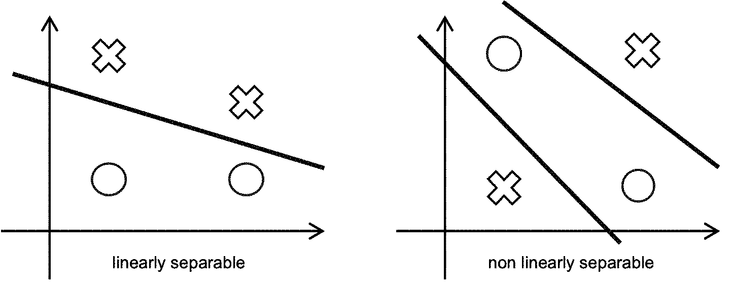
Neural networks reappeared in the 1980s, thanks to the idea of hidden layers joint with nonlinear units, to resolve the initial linear separability limitation, and to the backpropagation algorithm, to train such multilayer neural networks [167].
In the 1990s, neural networks suffered declining interest9898 98 Meanwhile, convolutional networks started to gain interest, notably though handwritten digit recognition applications [112]. As Goodfellow et al. in (63, Section 9.11) put it: “In many ways, they carried the torch for the rest of deep learning and paved the way to the acceptance of neural networks in general.” because of the difficulty in training efficiently neural networks with many layers9999 99 Another related limitation, although specific to the case of recurrent networks, was the difficulty in training them efficiently on very long sequences. This was resolved in 1997 by Hochreiter and Schmidhuber with the Long short-term memory (LSTM) architecture [83], presented in Section 25.3. and due to the competition from support vector machines (SVM) [197], which were efficiently designed to maximize the separation margin and had a solid formal background.
An important advance was the invention of the pre-training technique100100 100 Pre-training consists in prior training in cascade (one layer at a time, also named greedy layer-wise unsupervised training) of each hidden layer [80] (63, page 528). It turned out to be a significant improvement for the accurate training of neural networks with several layers [47]. That said, pre-training is now rarely used and has been replaced by other more recent techniques, such as batch normalization and deep residual learning. But its underlying techniques are useful for addressing some new concerns like transfer learning, which deals with the issue of reusability (of what has been learnt, see Section 54). by Hinton et al. in 2006 [80], which resolved this limitation. In 2012, an image recognition competition (the ImageNet Large Scale Visual Recognition Challenge [168]) was won by a deep neural network algorithm named AlexNet101101 101 AlexNet was designed by the SuperVision team headed by Hinton and composed of Alex Krizhevsky, Ilya Sutskever and Geoffrey E. Hinton [104]. AlexNet is a deep convolutional neural network with 60 million parameters and 650,000 neurons, consisting of five convolutional layers, some followed by max-pooling layers, and three globally-connected layers., with a stunning margin102102 102 On the first task, AlexNet won the competition with a 15% error rate whereas other teams did not achieve better than a 26% error rate. over the other algorithms which were using handcrafted features. This striking victory was the event which ended the prevalent opinion that neural networks with many hidden layers could not be efficiently trained103103 103 Interestingly, the title of Hinton et al.’s article about pre-training [80] is about ‘‘deep belief nets’’ and does not mention the term ‘‘neural nets” because, as Hinton remembers it in [106]: “At that time, there was a strong belief that deep neural networks were no good and could never be trained and that ICML (International Conference on Machine Learning) should not accept papers about neural networks.”.
18 Introduction to Neural Networks
The purpose of this section is to review, or to introduce, the basic principles of artificial neural networks. Our objective is to define the key concepts and terminology that we will use when analyzing various music generation systems. Then, we will introduce the concepts and basic principles of various derived architectures, like autoencoders, recurrent networks, RBMs, etc., which are used in musical applications. We will not describe extensively the techniques of neural networks and deep learning, for example covered in the recent book [63].
18.1 Linear Regression
Although bio-inspired (biological neurons), the foundation of neural networks and deep learning is linear regression. In statistics, linear regression is an approach for modeling the (assumed linear) relationship between a scalar variable and one104104 104 The case of one explanatory variable is called simple linear regression, otherwise it is named multiple linear regression. or more than one explanatory variable(s) x1 … xn, with x, jointly noted as vector x. A simple example is to predict the value of a house, depending on some factors (e.g., size, height, location…).
Equation 1 gives the general model of a (multiple) linear regression, where
| (1) |
- •
is the model, also named hypothesis, as this is the hypothetical best model to be discovered, i.e. learnt;
- •
is the bias105105 105 It could also be notated as , see Section 18.5., representing the offset; and
- •
… are the parameters of the model, the weights, corresponding to the explanatory variables x1 … xn.
18.2 Notations
We will use the following simple notation conventions
- •
a constant is in roman (straight) font, e.g., integer 1 and note C4.
- •
a variable of a model is in roman font, e.g., input variable x and output variable y (possibly vectors).
- •
a parameter of a model is in italics, e.g., bias , weight parameter , model function , number of explanatory variables and index of a variable xi.
- •
a probability as well as a probability distribution are in italics and upper case, e.g., probability that the value of variable note is A4 and probability distribution of variable note over all possible notes (outcomes).
18.3 Model Training
The purpose of training a linear regression model is to find the values for each weight and the bias that best fit the actual training data/examples, i.e. various pairs of values . In other words, we want to find the parameters and bias values such that for all values of x, is as close as possible106106 106 Actually, for the neural networks that are more complex (nonlinear models) than linear regression and that will be introduced in Section 22, the best fit to the training data is not necessarily the best hypothesis because it may have a low generalization, i.e. a low ability to predict yet unseen data. This issue, named overfitting, will be introduced in Section 22.9. to y, according to some measure named the cost. This measure represents the distance between (the prediction, also notated as ŷ) and y (the actual ground value), for all examples.
The cost, also named the loss, is usually107107 107 Or also , or . notated and could be measured, for example, by a mean squared error (MSE), which measures the average squared difference, as shown in Equation 2, where is the number of examples and is the th example pair.
| (2) |
An example is shown in Figure 18 for the case of simple linear regression, i.e. with only one explanatory variable x. Training data are shown as blue solid dots. Once the model has been trained, values of the parameters are adjusted, illustrated by the blue solid bold line which mostly fits the examples. Then, the model can be used for prediction, e.g., to provide a good estimate ŷ of the actual value of y for a given value of x by computing (shown in green).

18.4 Gradient Descent Training Algorithm
The basic algorithm for training a linear regression model, using the simple gradient descent method, is actually pretty simple108108 108 See, e.g., [142] for more details.:
- •
initialize each parameter and the bias to a random or some heuristic value109109 109 Pre-training led to a significant advance, as it improved the initialization of the parameters by using actual training data, via sequential training of the successive layers [47].;
- •
compute the values of the model for all examples110110 110 Computing the cost for all examples is the best method but also computationally costly. There are numerous heuristic alternatives to minimize the computational cost, e.g., stochastic gradient descent (SGD), where one example is randomly chosen, and minibatch gradient descent, where a subset of examples is randomly chosen. See, for example, (63, Sections 5.9 and 8.1.3) for more details.;
- •
compute the cost , e.g., by Equation 2;
- •
compute the gradients which are the partial derivatives of the cost function with respect to each , as well as to the bias ;
- •
update simultaneously111111 111 A simultaneous update is necessary for the algorithm to behave correctly. all parameters and the bias according to the update rule112112 112 The update rule may also be notated as , where is the vector of gradients . shown in Equation 3, with being the learning rate.
(3) This represents an update in the opposite direction of the gradients in order to decrease the cost , as illustrated in Figure 19; and
- •
iterate until the error reaches a minimum113113 113 If the cost function is convex (the case for linear regression), there is only one global minimum, and thus there is a guarantee of finding the optimal model., or after a certain number of iterations.

18.5 From Model to Architecture
Let us now introduce in Figure 20 a graphical representation of a linear regression model, as a precursor of a neural network. The architecture represented is actually the computational representation of the model114114 114 We mostly use the term architecture as, in this book, we are concerned with the way to implement and compute a given model and also with the relation between an architecture and a representation..
The weighted sum is represented as a computational unit115115 115 We use the term node for any component of a neural network, whether it is just an interface (e.g., an input node) or a computational unit (e.g., a weighted sum or a function). We use the term unit only in the case of a computational node. The term neuron is also often used in place of unit, as a way to emphasize the inspiration from biological neural networks., drawn as a squared box with a , taking its inputs from the xi nodes, drawn as circles.
In the example shown, there are four explanatory variables: x1, x2, x3 and x4. Note that there is some convention of considering the bias as a special case of weight (thus alternatively notated as ) and having a corresponding input node named the bias node, which is implicit116116 116 However, as will be explained later in Section 22, bias nodes rarely appear in illustrations of non-toy neural networks. and has a constant value notated as . This actually corresponds to considering an implicit additional explanatory variable x0 with constant value +1, as shown in Equation 4, alternative formulation of linear regression initially defined in Equation 1.
| (4) |

18.6 From Model to Linear Algebra Representation
The initial linear regression equation (in Equation 1) may also be made more compact thanks to a linear algebra notation leading to Equation 5 where
| (5) |
- •
and are scalars;
- •
is a row vector117117 117 That is a matrix which has a single row, i.e. a matrix of dimension . consisting of a single row of elements: ;
- •
x is a column vector118118 118 That is a matrix which has a single column, i.e. a matrix of dimension . consisting of a single column of elements: .
18.7 From Simple to Multivariate Model
Linear regression can be generalized to multivariate linear regression, the case when there are multiple variables y1 … yp to be predicted, as illustrated in Figure 21 with three predicted variables: y1, y2 and y3, each subnetwork represented in a different color.

The corresponding linear algebra equation is Equation 6, where
| (6) |
- •
the bias vector is a column vector of dimension , with representing the weight of the connexion between the bias input node and the th sum operation corresponding to the th output node;
- •
the weight matrix is a matrix of dimension , that is with rows and columns, with representing the weight of the connexion between the th input node and the th sum operation corresponding to the th output node;
- •
is the number of input nodes (without considering the bias node); and
- •
is the number of output nodes.
For the architecture shown in Figure 21, (the number of input nodes and of columns of ) and (the number of output nodes and of rows of ). The corresponding bias vector and weight matrix are shown in Equations 7 and 8119119 119 Indeed, and are generalizations of and for the case of univariate linear regression (as shown in Section 18.6) to the case of multivariate and thus to multiple rows, each row corresponding to an output node. and120120 120 By showing only the connexions to one of the output node, in order to keep readability. in Figure 22.

| (7) |
| (8) |
18.8 Activation Function
Let us now also apply an activation function (AF) to each weighted sum unit, as shown in Figure 23.

This activation function allows us to introduce arbitrary nonlinear functions.
- •
From an engineering perspective, a nonlinear function is necessary to overcome the linear separability limitation of the single layer Perceptron (see Section id1).
- •
From a biological inspiration perspective, a nonlinear function can capture the threshold effect for the activation of a neuron through its incoming signals (via its dendrites), determining whether it fires along its output (axone).
- •
From a statistical perspective, when the activation function is the sigmoid function, a model corresponds to logistic regression, which models the probability of a certain class or event and thus performs binary classification121121 121 For each output node/variable. See more details in Section 22.3..
Historically speaking, the sigmoid function (which is used for logistic regression) is the most common. The sigmoid function (usually written ) is defined in Equation 9 and is shown in Figure 24. It will be further analyzed in Section 22.3.
An alternative is the hyperbolic tangent, often noted tanh, similar to sigmoid but having as its domain interval ( for sigmoid). Tanh is defined in Equation 10 and shown in Figure 25.
But ReLU is now widely used for its simplicity and effectiveness. ReLU, which stands for rectified linear unit, is defined in Equation 9 and is shown in Figure 26. Note that, as some notation convention we use z as the name of the variable of an activation function, as x is usually reserved for input variables.
| (9) |

| (10) |

| (11) |

19 Basic Building Block
The architectural representation (of multivariate linear regression with activation function) shown in Figure 23 is an instance (with 4 input nodes and 3 output nodes) of a basic building block of neural networks and deep learning architectures. Although simple, this basic building block is actually a working neural network.
It has two layers122122 122 Although, as we will see in Section 22.2, it will be considered as a single-layer neural network architecture. As it has no hidden layer, it still suffers from the linear separability limitation of the Perceptron.:
- •
The input layer, on the left of the figure, is composed of the input nodes xi and the bias node which is an implicit and specific input node with a constant value of , therefore usually denoted as .
- •
The output layer, on the right of the figure, is composed of the output nodes yj.
Training a basic building block is essentially the same as training a linear regression model, which has been described in Section 18.3.
19.1 Feedforward Computation
After it has been trained, we can use this basic building block neural network for prediction. Therefore, we simply feedforward the network, i.e. provide input data to the network (feed in) and compute the output values. This corresponds to Equation 12.
| (12) |
The feedforward computation of the prediction (for the architecture shown in Figure 21) is illustrated in Equation 13, where (i.e. ŷj) is the prediction of the th variable .
| (13) |
19.2 Computing Multiple Input Data Simultaneously
Feedforwarding simultaneously a set of examples is easily expressed as a matrix by matrix multiplication, by substituting the single vector example x in Equation 12 with a matrix of examples (usually notated as X), leading to Equation 14.
Successive columns of the matrix of examples X correspond to the different examples. We use a superscript notation X(k) to denote the th example, the th column of the X matrix, to avoid confusion with the subscript notation xi which is used to denote the th input variable. Therefore, X denotes the th input value of the th example. The feedforward computation of a set of examples is illustrated in Equation 15, with predictions being successive columns of the resulting output matrix.
| (14) |
| (15) |
Note that the main computation taking place123123 123 Apart from the computation of the activation function. In the case of ReLU this is fast. is a product of matrices. This can be computed very efficiently, by using linear algebra vectorized implementation libraries and furthermore with specialized hardware like graphics processing units (GPUs).
20 Machine Learning
20.1 Definition
Let us now reflect a bit on the meaning of training a model, whether it is a linear regression model (Section 18.1) or the basic building block architecture presented in Section 19. Therefore, let us consider what machine learning actually means. Our starting point is the following concise and general definition of machine learning provided by Mitchell in [132]: “A computer program is said to learn from experience with respect to some class of tasks and performance measure , if its performance at tasks in , as measured by , improves with experience .”
At first, note that the word performance actually covers different meanings, specially regarding the computer music context of the book:
- 1.
the execution of (the action to perform) an action, notably an artistic act such as a musician playing a piece of music;
- 2.
a measure (criterium of evaluation) of that action, notably for a computer system its efficiency in performing a task, in terms of time and memory124124 124 With the corresponding analysis measurements, time complexity and space complexity, for the corresponding algorithms. measurements; or
- 3.
a measure of the accuracy in performing a task, i.e. the ability to predict or classify with minimal errors.
In the remainder of the book, in order to try to minimize ambiguity, we will use the terms as following:
- •
performance as an act by a musician,
- •
efficiency as a measure of computational ability, and
- •
accuracy as a measure of the quality of a prediction or a classification125125 125 In fact, accuracy may not be a pertinent metric for a classification task with skewed classes, i.e. with one class being vastly more represented in the data than other(s), e.g., in the case of the detection of a rare disease. Therefore a confusion matrix and additional metrics like precision and recall, and possible combinations like F-score, are used (see, e.g., (63, Section 11.1) for details). We will not address them in the book, because we are primarily concerned with content generation and not in pattern recognition (classification)..
Thus, we could rephrase the definition as: “A computer program is said to learn from experience with respect to some class of tasks and accuracy measure , if its accuracy at tasks in , as measured by , improves with experience .”
20.2 Categories
We may now consider the three main categories of machine learning with regard to the nature of the experience conveyed by the examples:
- •
supervised learning -- the dataset is fixed and a correct (expected) answer126126 126 It is usually named a label in the case of a classification task and a target in the case of a prediction/regression task. is associated to each example, the general objective being to predict answers for new examples. Examples of tasks are regression (prediction), classification and translation;
- •
unsupervised learning – the dataset is fixed and the general objective is in extracting information. Examples of tasks are feature extraction, data compression (both performed by autoencoders, to be introduced in Section 23), probability distribution learning (performed by RBMs, to be introduced in Section 24), series modeling (performed by recurrent networks, to be introduced in Section 25), clustering and anomaly detection; and
- •
reinforcement learning127127 127 To be introduced in Section 29. – the experience is incremental through successive actions of an agent within an environment, with some feedback (the reward) providing information about the value of the action, the general objective being to learn a near optimal policy (strategy), i.e. a suite of actions maximizing its cumulated rewards (its gain). Examples of tasks are game playing and robot navigation.
20.3 Components
In his introduction to machine learning [39], Domingos describes machine learning algorithms through three components:
- •
representation – the way to represent the model – in our case, a neural network, as it has been introduced and will be further developed in the following sections;
- •
evaluation – the way to evaluate and compare models – via a cost function, that will be analyzed in Section 22.4; and
- •
optimization – the way to identify (search among models for) a best model.
20.4 Optimization
Searching for values (of the parameters of a model) that minimize the cost function is indeed an optimization problem. One of the most simple optimization algorithms is gradient descent, as it has been introduced in Section 18.4.
There are various more sophisticated algorithms, such as stochastic gradient descent (SGD), Nesterov accelerated gradient (NAG), Adagrad, BFGS, etc. (see, for example, (63, Chapter 9) for more details).
21 Architectures
From this basic building block, we will describe in the following sections the main types of deep learning architectures used for music generation (as well as for other purposes):
- •
feedforward,
- •
autoencoder,
- •
restricted Boltzmann machine (RBM), and
- •
recurrent (RNN).
We will also introduce architectural patterns (see Section 30.1) which could be applied to them:
- •
convolutional,
- •
conditioning, and
- •
adversarial.
22 Multilayer Neural Network aka Feedforward Neural Network
A multilayer neural network, also named a feedforward neural network, is an assemblage of successive layers of basic building blocks:
- •
the first layer, composed of input nodes, is called the input layer;
- •
the last layer, composed of output nodes, is called the output layer; and
- •
any layer between the input layer and the output layer is named a hidden layer.
An example of a multilayer neural network with two hidden layers is illustrated in Figure 27.
The combination of a hidden layer and a nonlinear activation function makes the neural network a universal approximator, able to overcome the linear separability limitation128128 128 The universal approximation theorem [86] states that a feedforward network with a single hidden layer containing a finite number of neurons can approximate a wide variety of interesting functions when given appropriate parameters (weights). However, there is no guarantee that the neural network will be able to learn them!.

22.1 Abstract Representation
Note that, in the case of practical (non-toy) illustrations of neural network architectures, in order to simplify the figures, bias nodes are very rarely illustrated. With a similar objective, the sum units and the activation function units are also almost always omitted, resulting in a more abstract view such as that shown in Figure 28.

We can further abstract each layer by representing it as an oblong form (by hiding its nodes)129129 129 It is sometimes pictured as a rectangle, see Figure 30, or even as a circle, notably in the case of recurrent networks, see Figure 47. as shown in Figure 29.

22.2 Depth
The architecture illustrated in Figure 29 is called a 3-layer neural network architecture, also indicating that the depth of the architecture is three. Note that the number of layers (depth) is indeed three and not four, irrespective of the fact that summing up the input layer, the output layer and the two hidden layers gives four and not three. This is because, by convention, only layers with weights (and units) are considered when counting the number of layers in a multilayer neural network; therefore, the input layer is not counted. Indeed, the input layer only acts as an input interface, without any weight or computation.
In this book, we will use a superscript (power) notation130130 130 The set of compact notations for expressing the dimension of an architecture or a representation will be introduced in Section 31. to denote the number of layers of a neural network architecture. For instance, the architecture illustrated in Figure 29 could be denoted as Feedforward3.
The depth of the first neural network architectures was small. The original Perceptron [166], the ancestor of neural networks, has only an input layer and an output layer without any hidden layer, i.e. it is a single-layer neural network. In the 1980s, conventional neural networks were mostly 2-layer or 3-layer architectures.
For modern deep networks, the depth can indeed be very large, deserving the name of deep (or even very deep) networks. Two recent examples, both illustrated in Figure 30, are


- •
the 27-layer GoogLeNet architecture [182]; and
- •
Note that depth does matter. A recent theorem [44] states that there is a simple radial function132132 132 A radial function is a function whose value at each point depends only on the distance between that point and the origin. More precisely, it is radial if and only if it is invariant under all rotations while leaving the origin fixed. on , expressible by a 3-layer neural network, which cannot be approximated by any 2-layer network to more than a constant accuracy unless its width is exponential in the dimension . Intuitively, this means that reducing the depth (removing a layer) means exponentially augmenting the width (the number of units) of the layer left. On this issue, the interested reader may also wish to review the analyses in [4] and [193].
Note that for both networks pictured in Figure 30, the flow of computation is vertical, upward for GoogLeNet and downward for ResNet. These are different usages than the convention for the flow of computation that we have introduced and used so far, which is horizontal, from left to right. Unfortunately, there is no consensus in the literature about the notation for the flow of computation. Note that in the specific case of recurrent networks, to be introduced in Section 25, the consensus notation is vertical, upward.
22.3 Output Activation Function
We have seen in Section 19 that, in modern neural networks, the activation function () chosen for introducing nonlinearity at the output of each hidden layer is often the ReLU function. But the output layer of a neural network has a special status. Basically, there are three main possible types of activation function for the output layer, named in the following, the output activation function133133 133 A shorthand for output layer activation function.:
- •
identity -- the case for a prediction (regression) task. It has continuous (real) output values. Therefore, we do not need and we do not want a nonlinear transformation at the last layer;
- •
sigmoid -- the case of a binary classification task, as in logistic regression134134 134 For details about logistic regression, see, for example, (63, page 137) or (73, Section 4.4). For this reason, the sigmoid function is also called the logistic function.. The sigmoid function (usually written ) has been defined in Equation 9 and shown in Figure 24. Note its specific shape, which provides a “separation” effect, used for binary decision between two options represented by values and ; and
- •
softmax -- the most common approach for a classification task with more than two classes but with only one label to be selected135135 135 A very common example is the estimation by a neural network architecture of the next note, modeled as a classification task of a single note label within the set of possible notes. (and where a one-hot encoding is generally used, see Section 16).
The softmax function actually represents a probability distribution over a discrete output variable with possible values (in other words, the probability of the occurrence of each possible value , knowing the input variable x, i.e. ). Therefore, softmax ensures that the sum of the probabilities for each possible value is equal to . The softmax function is defined in Equation 16 and an example of its use is shown in Equation 17. Note that the notation is used for the softmax function, as for the sigmoid function, because softmax is actually the generalization of sigmoid to the case of multiple values, being a variadic function, that is one which accepts a variable number of arguments.
| (16) |
| (17) |
For a classification or prediction task, we can simply select the value with the highest probability (i.e. via the argmax function, the indice of the one-hot vector with the highest value). But the distribution produced by the softmax function can also be used as the basis for sampling, in order to add nondeterminism and thus content variability to the generation (this will be detailed in Section 36).
22.4 Cost Function
The choice of a cost (loss) function is actually correlated to the choice of the output activation function and to the choice of the encoding of the target y (the true value). Table 1136136 136 Inspired by Ronaghan’s concise pedagogical presentation in [165]. summarizes the main cases.
| Task | Type of the output (ŷ) | Encoding of | Output activation | Cost (loss) |
| the target (y) | function | |||
| Regression | Real | Identity (Linear) | Mean squared error | |
| Classification | Binary | {0, 1} | Sigmoid | Binary cross-entropy |
| Classification | Multiclass single label | One-hot | Softmax | Categorical cross-entropy |
| Classification | Multiclass multilabel | Many-hot | Sigmoid | Binary cross-entropy |
| Multiple | Multi | Multi | Sigmoid | Binary cross-entropy |
| Classification | Multiclass single label | One-hot | Multi | Multi |
| Softmax | Categorical cross-entropy |
A cross-entropy function measures the difference between two probability distributions, in our case (of a classification task) between the target (true value) distribution (y) and the predicted distribution (ŷ). Note that there are two types of cross-entropy cost functions:
- •
binary cross-entropy, when the classification is binary (Boolean), and
- •
categorical cross-entropy, when the classification is multiclass with a single label to be selected.
In the case of a classification with multiple labels, binary cross-entropy must be chosen joint with sigmoid (because in such cases we want to compare the distributions independently, class per class137137 137 In case of multiple labels, the probability of each class is independent from the other class probabilities – the sum is greater than 1.) and the costs for each class are summed up.
In the case of multiple simultaneous classifications (multi multiclass single label), each classification is now independent from the other classifications, thus we have two approaches: apply sigmoid and binary cross-entropy for each element and sum up the costs, or apply softmax and categorical cross-entropy independently for each classification and sum up the costs.
22.5 Interpretation
Let us take some examples to illustrate these subtle but important differences, starting with the cases of real and binary values in Figure 31. They also include the basic interpretation of the result138138 138 The interpretation is actually part of the strategy of the generation of music content. It will be explored in Chapter id1. For instance, sampling from the probability distribution may be used in order to ensure content generation variability, as will be explained in Section 36..

- •
- •
- •
An example of use of the multi multiclass single label type is a multiple classification among a set of possible notes for multivoice monophonic melodies, therefore with only one single possible note choice for each voice, as shown in Figure 34. See, for example, the BluesMC system in Section 35.1.2.
- •
Another example of use of the multi multiclass single label type is a multiple classification among a set of possible notes for a set of time steps (in a piano roll representation) for a monophonic melody, therefore with only one single possible note choice for each time step. See, for example, the DeepHearM system in Section 34.1.1.
- •
An example of use of a multi2 multiclass single label type is a 2-level multiple classification among a set of possible notes for a set of time steps for a multivoice set of monophonic melodies. See, for example, the MiniBach system in Section 32.2.


The three main interpretations used139139 139 In various systems to be analyzed in Chapter id1. are
- •
argmax (the index of the output vector with the largest value), in the case of a one-hot multiclass single label (in order to select the most likely note),
- •
sampling from the probability represented by the output vector, in the case of a one-hot multiclass single label (in order to select a note sorted along its likelihood), and
- •
argsort140140 140 argsort is a numpy library Python function. (the indexes of the output vector sorted according to their diminishing values), in the case of a many-hot multiclass multi label, filtered by some thresholds (in order to select the most likely notes above a probability threshold and under a maximum number of simultaneous notes).
22.6 Entropy and Cross-Entropy
Mean squared error has been defined in Equation 2 in Section 18.3. Without getting into details about information theory, we now introduce the notion and the formulation of cross-entropy141141 141 With some inspiration from Preiswerk’s introduction in [156]..
The intuition behind information theory is that the information content about an event with a likely (expected) outcome is low, while the information content about an event with an unlikely (unexpected, i.e. a surprise) outcome is high.
Let us take the example of a neural network architecture used to estimate the next note of a melody. Suppose that the outcome is and that it has a probability . We can then introduce the self-information (notated ) of that event in Equation 18.
| (18) |
Remember that a probability is by definition within interval. If we look at -log function in Figure 35, we could see that its value is high for a low probability value (unlikely outcome) and its value is null for a probability value equal to 1 (certain outcome), which corresponds to the objective introduced above. Note that the use of a logarithm also makes self-information additive for independent events, i.e. .

Then, let us consider all possible outcomes , each outcome having as its associated probability, and being the probability distribution for all possible outcomes. The intuition is to define the entropy (notated ) of the probability distribution for all possible outcomes as the sum of the self-information for each possible outcome, weighted by the probability of the outcome. This leads to Equation 19.
| (19) |
Note that we can further rewrite the definition by using the notion of expectation142142 142 An expectation, or expected value, of some function with respect to a probability distribution , usually notated as , is the average (mean) value that takes on when x is drawn from , i.e. (we are here considering the case of discrete variables, which is the case for classification within a set of possible notes)., which leads to Equation 20.
| (20) |
Now, let us introduce in Equation 21 the Kullback-Leibler divergence (often abbreviated as KL-divergence, and notated ), as some measure143143 143 Note that it is not a true distance measure as it not symmetric. of how different are two separate probability distributions and over a same variable (note).
| (21) |
may be rewritten as in Equation 22144144 144 By using definition in Equation 20., where , named the categorical cross-entropy, is defined in Equation 23.
| (22) |
| (23) |
Note that categorical cross-entropy is similar to KL-divergence145145 145 And, just like KL-divergence, it is not symmetric., while lacking the term. But minimizing or minimizing , with respect to , are equivalent, because the omitted term is a constant with respect to .
Now, remember146146 146 See Section 22.4. that the objective of the neural network is to predict the ŷ probability distribution, which is an estimation of the y true ground probability distribution, by minimizing the difference between them. This leads to Equations 24 and 25.
| (24) |
| (25) |
As mentioned above, minimizing or minimizing , with respect to ŷ, are equivalent, because the omitted term is a constant with respect to ŷ.
Last, deriving the binary cross-entropy (that we notate ) is easy, as there are only two possible outcomes, which leads to Equation 26.
| (26) |
Because and (as the sum of the probabilities of the two possible outcomes is 1), this ends up into Equation 27.
| (27) |
More details and principles for the cost functions147147 147 The underlying principle of maximum likelihood estimation, not explained here. can be found, for example, in (63, Section 6.2.1) and (63, Section 5.5), respectively. In addition, the information theory foundation of cross-entropy as the number of bits needed for encoding information is introduced, for example, in [37].
22.7 Feedforward Propagation
Feedforward propagation in a multilayer neural network consists in injecting input data148148 148 The x part of an example, for the generation phase as well as for the training phase. into the input layer and propagating the computation through its successive layers until the output is produced. This can be implemented very efficiently because it consists in a pipelined computation of successive vectorized matrix products (intercalated with activation function calls).
Each computation from layer to layer is processed as in Equation 28, which is a generalization of Equation 12149149 149 Feedforward computation for one layer has been introduced in Section 19.1., where and 150150 150 We use a superscript notation with brackets [k] to denote the th layer, to avoid confusion with the superscript notation with parentheses (k) to denote the th example and the subscript notation i to denote the th input variable. are respectively the bias and the weight matrix between layer and layer , and where is the input layer, as shown in Figure 36.
| (28) |

Multilayer neural networks are therefore often also named feedforward neural networks or multilayer Perceptron (MLP)151151 151 The original Perceptron was a neural network with no hidden layer, and thus equivalent to our basic building block, with only one output node and with the step function as the activation function..
Note that neural networks are deterministic. This means that the same input will deterministically always produce the same output. This is a useful guarantee for prediction and classification purposes but may be a limitation for generating new content. However, this may be compensated by sampling from the resultant probability distribution (see Sections 22.3 and 36).
22.8 Training
For the training phase152152 152 Let us remember that this a case of supervised learning (see Section 19)., computing the derivatives becomes a bit more complex than for the basic building block (with no hidden layer) presented in Section 18.4. Backpropagation is the standard method of estimating the derivatives (gradients) for a multilayer neural network. It is based on the chain rule principle [167], in order to estimate the contribution of each weight to the final prediction error, that is the cost. See, for example, (63, Chapter 6) for more details.
Note that, in the most common case, the cost function of a multilayer neural network is not convex, meaning that there may be multiple local minima. Gradient descent, as well as other more sophisticated heuristic optimization methods, does not guarantee the global optimum will be reached. But in practice a clever configuration of the model (notably, its hyperparameters, see Section 22.11) and well-tuned optimization heuristics, such as stochastic gradient descent (SGD), will lead to accurate solutions153153 153 On this issue, see [24], which shows that 1) local minima are located in a well-defined band, 2) SGD converges to that band, 3) reaching the global minimum becomes harder as the network size increases and 4) in practice this is irrelevant as the global minimum often leads to overfitting (see next section)..
22.9 Overfitting
A fundamental issue for neural networks (and more generally speaking for machine learning algorithms) is their generalization ability, that is their capacity to perform well on yet unseen data. In other words, we do not want a neural network to just perform well on the training data154154 154 Otherwise, the best and simpler algorithm would be a memory-based algorithm, which simply memorizes all (x, y) pairs. It has the best fit to the training data but it does not have any generalization ability. but also on future data155155 155 Future data is not yet known but that does not mean that it is any kind of (random) data, otherwise a machine learning algorithm would not be able to learn and generalize well. There is indeed a fundamental assumption of regularity of the data corresponding to a task (e.g., images of human faces, jazz chord progressions, etc.) that neural networks will exploit.. This is actually a fundamental dilemma, the two opposing risks being
- •
underfitting – when the training error (error measure on the training data) is large; and
- •
overfitting – when the generalization error (expected error on yet unseen data) is large.
A simple illustrative example of underfit, good fit and overfit models for the same training data (the green solid dots) is shown in Figure 37.

In order to be able to estimate the potential for generalization, the dataset is actually divided into two portions, with a ratio of approximately 70/30:
- •
the training set – which will be used for training the neural network; and
- •
the validation set, also named test set156156 156 Actually, a difference could (should) be made, as explained by Hastie et al. in (73, page 222): “It is important to note that there are in fact two separate goals that we might have in mind: Model selection: estimating the performance of different models in order to choose the best one. Model assessment: having chosen a final model, estimating its prediction error (generalization error) on new data. If we are in a data-rich situation, the best approach for both problems is to randomly divide the dataset into three parts: a training set, a validation set, and a test set. The training set is used to fit the models; the validation set is used to estimate prediction error for model selection; the test set is used for assessment of the generalization error of the final chosen model.” However, as a matter of simplification, we will not consider that difference in the book. – which will be used to estimate the capacity of the model for generalization.
22.10 Regularization
There are various techniques to control overfitting, i.e., to improve generalization. They are usually named regularization and some examples of well-known techniques are
- •
weight decay (also known as L2), by penalizing over-preponderant weights;
- •
dropout, by introducing random disconnections;
- •
early stopping, by storing a copy of the model parameters every time the error on the validation set reduces, then terminating after an absence of progress during a pre-specified number of iterations, and returning these parameters; and
- •
dataset augmentation, by data synthesis (e.g., by mirroring, translation and rotation for images; by transposition for music, see Section 17.1), in order to augment the number of training examples.
We will not further detail regularization techniques, see, for example, (63, Section 7).
22.11 Hyperparameters
In addition to the parameters of the model, which are the weights of the connexions between nodes, a model also includes hyperparameters, which are parameters at an architectural meta-level, concerning both structure and control.
Examples of structural hyperparameters, mainly concerned with the architecture, are
- •
number of layers,
- •
number of nodes, and
- •
nonlinear activation function.
Examples of control hyperparameters, mainly concerned with the learning process, are
- •
optimization procedure,
- •
learning rate, and
- •
regularization strategy and associated parameters.
Choosing proper values for (tuning) the various hyperparameters is fundamental both for the efficiency and the accuracy of neural networks for a given application. There are two approaches for exploring and tuning hyperparameters: manual tuning or automated tuning – by algorithmic exploration of the multidimensional space of hyperparameters and for each sample evaluating the generalization error. The three main strategies for automated tuning are
- •
random search – by defining a distribution for each hyperparameter, sampling configurations, and evaluating them;
- •
grid search – as opposed to random search, exploration is systematic on a small set of values for each hyperparameter; and
- •
model-based optimization – by building a model of the generalization error and running an optimization algorithm over it.
The challenge of automated tuning is its computational cost, although trials may be run in parallel. We will not detail these approaches here; however, further information can be found in (63, Section 11.4).
Note that this tuning activity is more objective for conventional tasks such as prediction and classification because the evaluation measure is objective, being the error rate for the validation set. When the task is the generation of new musical content, tuning is more subjective because there is no preexisting evaluation measure. It then turns out to be more qualitative, for instance through a manual evaluation of generated music by musicologists. This evaluation issue will be addressed in Section 57.
22.12 Platforms and Libraries
Various platforms157157 157 See, for example, the survey in [154]., such as CNTK, MXNet, PyTorch and TensorFlow, are available as a foundation for developing and running deep learning systems158158 158 There are also more general libraries for machine learning and data analysis, such as the SciPy library for the Python language, or the language R and its libraries.. They include libraries of
- •
basic architectures, such as the ones we are presenting in this chapter;
- •
components, for example optimization algorithms;
- •
runtime interfaces for running models on various hardware, including GPUs or distributed Web runtime facilities; and
- •
visualization and debugging facilities.
Keras is an example of a higher-level framework to simplify development, with CNTK, TensorFlow and Theano as possible backends. ONNX is an open format for representing deep learning models and was designed to ease the transfer of models between different platforms and tools.
23 Autoencoder
An autoencoder is a neural network with one hidden layer and with an additional constraint: the number of output nodes is equal to the number of input nodes159159 159 The bias is not counted/considered here as it is an implicit additional input node.. The output layer actually mirrors the input layer. It is shown in Figure 38, with its peculiar symmetric diabolo (or sand-timer) shape aspect.

Training an autoencoder represents a case of unsupervised learning, as the examples do not contain any additional label information (the effective value or class to be predicted). But the trick is that this is implemented using conventional supervised learning techniques, by presenting output data equal to the input data160160 160 This is sometimes called self-supervised learning [110].. In practice, the autoencoder tries to learn the identity function. As the hidden layer usually has fewer nodes than the input layer, the encoder component (shown in yellow in Figure 38) must compress information while the decoder (shown in purple) has to reconstruct, as accurately as possible, the initial information161161 161 Compared to traditional dimension reduction algorithms, such as principal component analysis (PCA), this approach has two advantages: 1) feature extraction is nonlinear (the case of manifold learning, see (63, Section 5.11.3) and Section 23.2) and 2) in the case of a sparse autoencoder (see next section), the number of features may be arbitrary (and not necessarily smaller than the number of input parameters).. This forces the autoencoder to discover significant (discriminating) features to encode useful information into the hidden layer nodes (also named the latent variables162162 162 In statistics, latent variables are variables that are not directly observed but are rather inferred (through a mathematical model) from other variables that are observed (directly measured). They can serve to reduce the dimensionality of data.). Therefore, autoencoders may be used to automatically extract high-level features [110]. The set of features extracted are often named an embedding163163 163 See the definition of embedding in Section 14.3.. Once trained, in order to extract features from an input, one just needs to feedforward the input data and gather the activations of the hidden layer (the values of the latent variables).
Another interesting use of decoders is the high-level control of content generation. The latent variables of an autoencoder constitute a compact representation of the common features of the learnt examples. By instantiating these latent variables and decoding the embedding, we can generate a new musical content corresponding to the values of the latent variables. We will explore this strategy in Section 34.1.
23.1 Sparse Autoencoder
A sparse autoencoder is an autoencoder with a sparsity constraint, such that its hidden layer units are inactive most of the time. The objective is to enforce the specialization of each unit in the hidden layer as a specific feature detector.
For instance, a sparse autoencoder with 100 units in its hidden layer and trained on 1010 pixel images will learn to detect edges at different positions and orientations in images, as shown in Figure 39. When applied to other input domains, such as audio or symbolic music data, this algorithm will learn useful features for those domains too.
The sparsity constraint is implemented by adding an additional term to the cost function to be minimized, see more details in [141] or (63, Section 14.2.1).
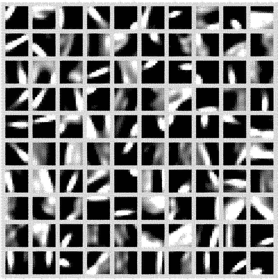
23.2 Variational Autoencoder
A variational autoencoder (VAE) [102] has the added constraint that the encoded representation, the latent variables, by convention denoted by variable z, follow some prior probability distribution . Usually, a Gaussian distribution164164 164 Also named normal distribution. is chosen for its generality.
This constraint is implemented by adding a specific term to the cost function, by computing the cross-entropy between the values of the latent variables and the prior distribution165165 165 The actual implementation is more complex and has some tricks (e.g., the encoder actually generates a mean vector and a standard deviation vector) that we will not detail here.. For more details about VAEs, an example of tutorial could be found in [38] and there is a nice introduction of its application to music in [162].
As with an autoencoder, a VAE will learn the identity function, but furthermore the decoder part will learn the relation between a Gaussian distribution of the latent variables and the learnt examples. As a result, sampling from the VAE is immediate, one just needs to
- •
sample a value for the latent variables , i.e. z following distribution ;
- •
input it into the decoder; and
- •
feedforward the decoder to generate an output corresponding to the distribution of the examples, following conditional probability distribution learnt by the decoder.
This is in contrast to the need for indirect and computationally expensive strategies such as Gibbs sampling for other architectures such as RBM, to be introduced in Section 24.
By construction, a variational autoencoder is representative of the dataset that it has learnt, that is, for any example in the dataset, there is at least one setting of the latent variables which causes the model to generate something very similar to that example [38].
A very interesting characteristic of the variational autoencoder architecture for generation purposes – therefore often considered as one type of a class of models named generative models -- is in the meaningful exploration of the latent space, as a variational autoencoder is able to learn a ‘‘smooth’’166166 166 That is, a small change in the latent space will correspond to a small change in the generated examples, without any discontinuity or jump. For a more detailed discussion about which (and how) interesting effects (smoothness, parsimony and axis-alignment between data and latent variability) a VAE has on the latent representation (the vector of latent variables) learnt, see, e.g., [206]. latent space mapping to realistic examples. Note that this general objective is named manifold learning and more generally representation learning [8], that is the learning of a representation capturing the topology of a set of examples. As defined in (63, Section 5.11.3), a manifold is a connected set of points (examples) that can be approximated by a smaller number of dimensions, each one corresponding to a local direction of variation. An intuitive example is a 2D map capturing the topology of cities dispersed on the 3D earth, where a movement on the map corresponds to a movement on the earth.
To illustrate the possibilities, let us train a VAE with only two latent variables on the MNIST handwritten digits database dataset [113] (with 60.000 examples, each one being an image of 2828 pixels). Then, we scan the latent two-dimension plane, sampling latent values for the two latent variables (i.e. sampling points within the 2-dimension latent space) at regular intervals and generating the corresponding artificial digits by decoding the latent points167167 167 As proposed and implemented in [23].. Figure 40 shows examples of artificial digits generated.

Note that training the VAE has forced it to compress information about the actual examples by splitting (though the encoder) information in two subsets:
- •
the specific (discriminative) part, encoded within the latent variables; and
- •
the common part, encoded within the weights of the decoder, in order to be able to reconstruct as close as possible each original data168168 168 Indeed, there is no magic here, the reversible compression from 2828 variables to 2 variables must have extracted and stored missing information somewhere..
The VAE actually has been forced to find out dimensions of variations for the dataset examples. By looking at the figure, we can guess that the two dimensions could be:
- •
from angular to round elements for the 1st variable (z1, horizontally represented), and
- •
the size of the compound element (circle or angle) for the second latent variable (z2, vertically represented).
Note that we cannot expect/force the VAE towards the semantics (meaning) of specific dimensions, as the VAE will automatically extract them (this depends on the dataset as well as on the training configuration), and we can only try to interpret them a posteriori169169 169 However, we will see that we can construct arbitrary characteristic attributes from a subset of examples and impose them on other examples, by doing attribute vector arithmetics, as defined in the immediately following list, and as will be illustrated in Figure 132 in Section 42.1.. Examples of possible dimensions for music generation could be: the number of notes170170 170 This will be illustrated in Figure 92 in Section 40.2.3., the range (the distance from the lowest to the highest pitch), etc.
Once learnt by a VAE, the latent representation (a vector of latent variables) can be used to explore the latent space with various operations to control/vary the generation of content. Some examples of operations on the latent space, as proposed in [162] and [163] for the MusicVAE system described in Section 42.1, are
- •
translation;
- •
interpolation;
- •
averaging of some points;
- •
attribute vector arithmetics, by addition or subtraction of an attribute vector capturing a given characteristic171171 171 This attribute vector is computed as the average latent vector for a collection of examples sharing that attribute (characteristic)..
Figure 41 shows an interesting comparison of melodies resulting from

- •
interpolation in the data space, that is the space of representation of melodies; and
- •
interpolation in the latent space, which is then decoded into the corresponding melodies.
The interpolation in the latent space produces more meaningful and interesting melodies than the interpolation in the data space (which basically just varies the ratio of notes from the two melodies), as can be heard in [161] and [164]. More details about these experiments will be provided in Section 42.1.
23.3 Stacked Autoencoder
The idea of a stacked autoencoder is to hierarchically nest successive autoencoders with decreasing numbers of hidden layer units. An example of a 2-layer stacked autoencoder172172 172 Note that the convention in this case is to count and notate the number of nested autoencoders, i.e. the number of hidden layers. This is different from the depth of the whole architecture, which is double. For instance, a 2-layer stacked autoencoder results in a 4-layer whole architecture, as shown in Figure 42., i.e. two nested autoencoders that we could notate as Autoencoder2, is illustrated in Figure 42.

The chain of encoders will increasingly compress data and extract higher-level features. Stacked autoencoders, which are indeed deep networks, are therefore used for feature extraction (an example will be introduced in Section 40.7.1). They are also useful for music generation, as we will see in Section 34.1. This is because the innermost hidden layer, sometimes named the bottleneck hidden layer, provides a compact and high-level encoding (embedding) as a seed for generation (by the chain of decoders).
24 Restricted Boltzmann Machine (RBM)
A restricted Boltzmann machine (RBM) [81] is a generative stochastic artificial neural network that can learn a probability distribution over its set of inputs. Its name comes from the fact that it is a restricted (constrained) form173173 173 Which actually makes RBM practical, as opposed to the general form, which besides its interest suffers from a learning scalability limitation. of a (general) Boltzmann machine [82], named after the Boltzmann distribution in statistical mechanics, which is used in its sampling function. The architectural restrictions of an RBM (see Figure 43) are that
- •
it is organized in layers, just as for a feedforward network or an autoencoder, and more precisely two layers:
- –
the visible layer (analog to both the input layer and the output layer of an autoencoder); and
- –
the hidden layer (analog to the hidden layer of an autoencoder);
- –
- •
as for a standard neural network, there cannot be connections between nodes within the same layer.

An RBM bears some similarity in spirit and objective to an autoencoder. However, there are some important differences:
- •
an RBM has no ouput – the input also acts as the output;
- •
an RBM is stochastic (and therefore not deterministic, as opposed to a feedforward network or an autoencoder);
- •
an RBM is trained in an unsupervised learning manner, with a specific algorithm (named contrastive divergence, see Section 24.1), whereas an autoencoder is trained using a standard supervised learning method, with the same data as input and output; and
- •
the values manipulated are booleans174174 174 Although there are extensions with multinoulli (categorical) or continuous values, see Section 24.3..
RBMs became popular after Hinton designed a specific fast learning algorithm for them, named contrastive divergence [79], and used them for pre-training deep neural networks [47] (see Section id1).
An RBM is an architecture dedicated to learning distributions. Moreover, it can learn efficiently from only a few examples. For musical applications, this is interesting for learning (and generating) chords, as the combinatorial nature of possible notes forming a chord is large and the number of examples is usually small. We will see an example of such an application in Section 34.2.3.
24.1 Training
Training an RBM has some similarity to training an autoencoder, with the practical difference that, because there is no decoder part, the RBM will alternate between two steps:
- •
the feedforward step – to encode the input (visible layer) into the hidden layer, by making predictions about hidden layer node activations; and
- •
the backward step – to decode/reconstruct the input (visible layer), by making predictions about visible layer node activations.
We will not detail here the learning technique behind RBMs, see, for example, (63, Section 20.2). Note that the reconstruction process is an example of generative learning (and not discriminative learning, as for training autoencoders which is based on regression)175175 175 See, for example, a nice introduction to generative learning (and the difference with discriminative learning) in [143]..
24.2 Sampling
After the training phase has been completed, in the generation phase, a sample can be drawn from the model by randomly initializing visible layer vector (following a standard uniform distribution) and running sampling176176 176 More precisely Gibbs sampling (GS), see [107]. Sampling will be introduced in Section 34.2.1. until convergence. To this end, hidden nodes and visible nodes are alternately updated (as during the training phase).
In practice, convergence is reached when the energy stabilizes. The energy of a configuration (the pair of visible and hidden layers) is expressed177177 177 For more details, see, for example, (63, Section 16.2.4). in the Equation 29, where
| (29) |
- •
v and h, respectively, are column vectors representing the visible and the hidden layers;
- •
is the matrix of weights associated with the connections between visible and hidden nodes;
- •
and , respectively, are column vectors representing the bias weights for visible and hidden nodes, with and being their respective transpositions into row vectors; and
- •
is the transposition of v into a row vector.
24.3 Types of Variables
Note that there are actually three possibilities for the nature of RBM variables (units, visible or hidden):
- •
Boolean or Bernoulli -- this is the case of standard RBMs, in which units (visible and hidden) are Boolean, with a Bernoulli distribution (see (63, Section 3.9.2));
- •
multinoulli – an extension with multinoulli units178178 178 As explained by Goodfellow et al. in (63, Section 3.9.2): ““Multinoulli” is a term that was recently coined by Gustavo Lacerdo and popularized by Murphy in [140]. The multinoulli distribution is a special case of the multinomial distribution. A multinomial distribution is the distribution over vectors in representing how many times each of the categories is visited when samples are drawn from a multinoulli distribution. Many texts use the term “multinomial” to refer to multinoulli distributions without clarifying that they refer only to the case.”, i.e. with more than two possible discrete values; and
- •
continuous -- another extension with continuous units, taking arbitrary real values (usually within the range). An example is the C-RBM architecture analyzed in Section 40.5.1.
25 Recurrent Neural Network (RNN)
A recurrent neural network (RNN) is a feedforward neural network extended with recurrent connexions in order to learn series of items (e.g., a melody as a sequence of notes). The input of the RNN is an element xt179179 179 This xt notation – or sometimes st to stress the fact that it is a sequence – is very common but unfortunately introduces possible confusion with the notation of xi as the th input variable. The context – recurrent versus nonrecurrent network – usually helps to discriminate, as well as the use of the letter (for time) as the index. An example of an exception is the RNN-RBM system analyzed in Section 39.1, which uses the x(t) notation. of the sequence, where represents the index or the time, and the expected output is next element xt+1. In other words the RNN will be trained to predict the next element of a sequence.
In order to do so, the output of the hidden layer reenters itself as an additional input (with a specific corresponding weight matrix). This way, the RNN can learn, not only based on the current item but also on its previous own state, and thus, recursively, on the whole of the previous sequence. Therefore, an RNN can learn sequences, notably temporal sequences, as in the case of musical content.


An example of RNN (with two hidden layers) is shown in Figure 44. Recurrent connexions are signaled with a solid square, in order to distinguish them from standard connexions180180 180 Actually, there are some variations of this basic architecture, depending on the exact nature and location of the recurrent connexions. The most standard case is a recurrent connexion for each hidden unit, as shown in Figure 44. But there are some other cases, see for example in (63, Section 10.2). An example of a music generation architecture with recurrent connexions from the output to a special context input will be introduced in Section 38.2.. The unfolded version of the visual representation is in Figure 45, with a new diagonal axis representing the time dimension, in order to illustrate the previous step value of each layer (in thinner and lighter color). Note that, as for standard connexions (shown in yellow solid lines), recurrent connexions (shown in purple dashed lines) fully connect (with a specific weight matrix) all nodes corresponding to the previous step nodes to the nodes corresponding to the current step, as illustrated in Figure 46.

An RNN can learn a probability distribution over a sequence by being trained to predict the next element at time step in a sequence as being the conditional probability distribution , also notated as , that is the probability distribution given all previous elements generated s1, s2, … , st-1. In summary, recurrent networks (RNNs) are good at learning sequences and therefore are routinely used for natural text processing and for music generation.
25.1 Visual Representation
A more frequent visual representation for an RNN is actually showing the flow upwards and time rightwards, see the folded version (of an RNN with only one hidden layer) in Figure 47 and the unfolded version in Figure 48, with ht being the value of the hidden layer at step , and xt and yt being the values of the input and output at step .


25.2 Training
A recurrent network is not trained in exactly the same manner as a feedforward network. The idea is to present an example element of a sequence (e.g., a note within a melody) as the input xt and the next element of the sequence (the next note) xt+1 as the output yt. This will train the recurrent network to predict the next element of the sequence. In practice, an RNN is rarely trained element by element but with a sequence as an input and the same sequence shifted left by one step/item as the output. See an example in Figure 49181181 181 The end of the sequence is marked by a special symbol.. Therefore, the recurrent network will learn to predict182182 182 Pictured as dashed arrows. the next element for all successive elements of the sequence.

The backpropagation algorithm to compute gradients for feedforward networks, introduced in Section 22.8, has been extended into a backpropagation through time (BPTT) algorithm for recurrent networks. The intuition is in unfolding the RNN through time and considering an ordered sequence of input-output pairs, but with every unfolded copy of the network sharing the same parameters, and then applying the standard backpropagation algorithm. More details may be found, for example, in (63, Section 10.2.2).
Note that, a RNN has usually an output layer identical to its input layer183183 183 RNNs are actually more general and there are actually some rare cases of an RNN with an arbitrary output different from the input (as for a feedforward network). An example is a RNN-based architecture to generate a chord-based accompaniment, to be analyzed in Section 38.3. As Karpathy puts it in [98]: “Depending on your background you might be wondering: What makes Recurrent Networks so special? A glaring limitation of Vanilla Neural Networks (and also Convolutional Networks) is that their API is too constrained: they accept a fixed-sized vector as input (e.g. an image) and produce a fixed-sized vector as output (e.g. probabilities of different classes). Not only that: These models perform this mapping using a fixed amount of computational steps (e.g. the number of layers in the model). The core reason that recurrent nets are more exciting is that they allow us to operate over sequences of vectors: Sequences in the input, the output, or in the most general case both.”, as a recurrent network predicts the next item, which will be used iteratively as the next input in a recursive way in order to produce a sequence.
Note also that training a recurrent network is usually considered as a case of supervised learning as, for each item, the next item is presented as the expected prediction, although it is not an additional label information (effective value or class to be predicted) but only the recurrent information about the next item (intrinsically present within a sequence).
25.3 Long Short-Term Memory (LSTM)
Recurrent networks suffered from a training problem caused by the difficulty of estimating gradients because in backpropagation through time recurrence brings repetitive multiplications, and could thus lead to over amplify or minimize effects184184 184 This has been coined as the vanishing or exploding gradient problem and also as the challenge of long-term dependencies (see, for example, (63, Section 10.7)).. This problem has been addressed and resolved by the long short-term memory (LSTM) architecture, proposed by Hochreiter and Schmidhuber in 1997 [83]. As the solution has been quite effective, LSTM has become the de facto standard for recurrent networks185185 185 Although, there are a few subsequent but similar proposals, such as gated recurrent units (GRUs). See a comparative analysis of LSTM and GRU in [25]..
The idea behind LSTM is to secure information in memory cells, within a block186186 186 Cells within the same block share input, output and forget gates. Therefore, although each cell might hold a different value in its memory, all cell memories within a block are read, written or erased all at once [83]., protected from the standard data flow of the recurrent network. Decisions about writing to, reading from and forgetting (erasing) the values of cells within a block are performed by the opening or closing of gates and are expressed at a distinct control level (meta-level), while being learnt during the training process. Therefore, each gate is modulated by a weight parameter, and thus is suitable for backpropagation and standard training process. In other words, each LSTM block learns how to maintain its memory as a function of its input in order to minimize loss.
See a conceptual view of an LSTM cell in Figure 50. We will not further detail here the inner mechanism of an LSTM cell (and block) because we may consider it here as a black box (please refer to, for example, the original article [83]).

Note that a more general model of memory with access customized through training has recently been proposed: neural Turing machines (NTM) [66]. In this model, memory is global and has read and write operations with differentiable controls, and thus is subject to learning through backpropagation. The memory to be accessed, specified by location or by content, is controlled via an attention mechanism (introduced in next section).
25.4 Attention Mechanism
The motivation for an attention mechanism has been inspired by the human visual system ability to efficiently track and recognize objects by focusing its attention. It has therefore been first introduced into neural network architectures for image recognition, as for instance for object tracking [35]. It has then been adapted to recurrent architectures for natural language processing (and more specifically for translation tasks) and has showed significant improvement for the management of long-term dependencies.
The idea of an attention mechanism is to focus at each time step on some specific elements of the input sequence. This is modeled by weighted connexions onto the sequence elements (or onto the sequence of hidden units). Therefore it is differentiable and subject to backpropagation-based learning at a meta-level, as with LSTM gate control described in previous section. For more details, see, for example, (63, Section 12.4.5.1).
Interestingly, a novel architecture for translation of sequences, named Transformer and which is solely based on an attention mechanism187187 187 The architecture introduces multi-head attention which allows the model to jointly attend to information from different representation subspaces at different positions [198]., has recently being proposed and shows promising results [198]. Its very recent application to music generation will be shortly discussed in Section 53.
26 Convolutional Architectural Pattern
Convolutional neural network (CNN or ConvNet) architectures for deep learning have become common place for image applications. The concept was originally inspired by both a model of human vision and the convolution mathematical operator188188 188 In mathematics, a convolution is a mathematical operation on two functions sharing the same domain (usually noted ) that produces a third function which is the integral (or the sum in the discrete case – the case of images made of pixels) of the pointwise multiplication of the two functions varying within the domain in an opposing way. In the case of a continuous domain : In the discrete case: . It has been carefully adapted to neural networks and improved by LeCun, at first for handwritten character and object recognition [111]. This resulted in efficient and accurate architectures for pattern recognition, exploiting the spatial local correlation present in natural images.
26.1 Principles
The basic idea189189 189 Inspired by the nice intuitive explanation provided by Karn in [97]. For more technical details see, for example, [117] or (63, Chapter 9). is to
- •
slide a matrix (named a filter, a kernel or a feature detector) through the entire image (seen as the input matrix); and
- •
for each mapping position:
- –
compute the dot product of the filter with each mapped portion of the image; and
- –
then sum up all elements of the resulting matrix;
- –
- •
resulting in a new matrix (composed of the different sums for each sliding/mapping position), named convolved feature, or also feature map.
The size of the feature map is controlled by three hyperparameters:
- •
depth – the number of filters used;
- •
stride – the number of pixels by which we slide the filter matrix over the input matrix; and
- •
zero-padding -- the padding of the input matrix with zeros around its border190190 190 Zero-padding allows mapping of the filter up to the borders of the image. It also avoids shrinking the representation, which otherwise would be problematic when using multiple consecutive convolutional layers (63, Section 9.5)..
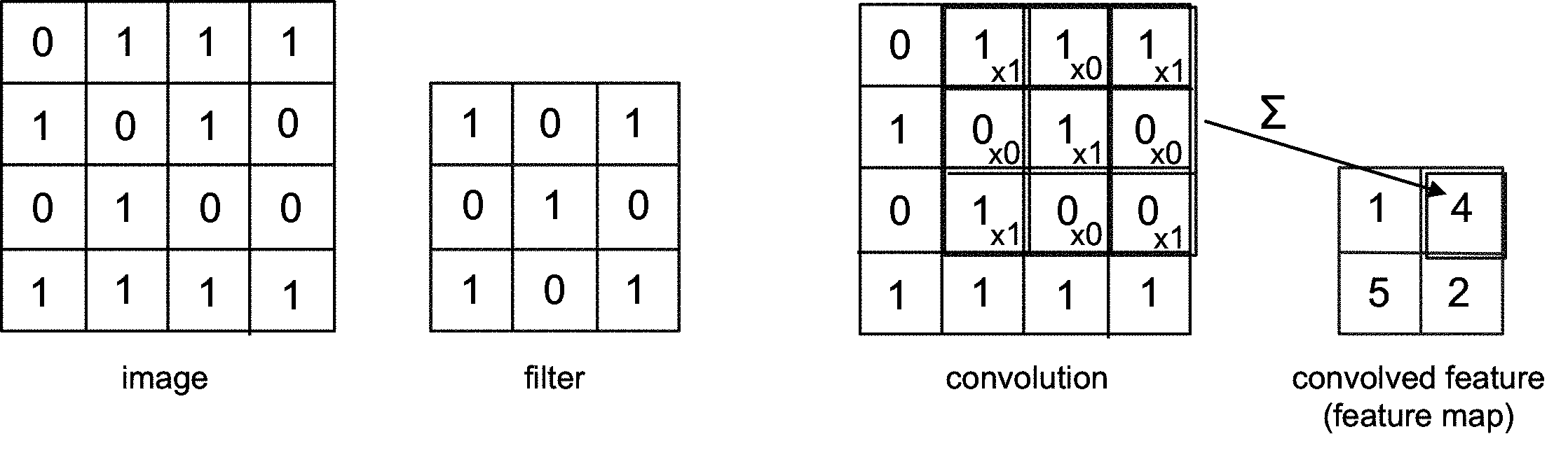
An example is illustrated in Figure 51 with some simple settings: depth = 1, stride = 1 and no zero-padding. Various filter matrixes can be used with different objectives, such as detection of different features (e.g., edges or curves) or other operations such as sharpening or blurring.
The parameter sharing used by the convolution (because of the shared fixed filter) brings the important property of equivariance to translation, i.e. a motif in an image can be detected independently of its location (63, Chapter 9).
26.2 Stages
A convolution usually consists of three successive stages:
- •
a convolution stage, as described in Section 26.1;
- •
a nonlinear rectification stage, sometimes named detector stage, which applies a nonlinear operation, usually ReLU; and
- •
a pooling stage, also named subsampling, to reduce the dimensionality.
26.3 Pooling
The motivation for pooling is to reduce the dimensionality of each feature map while retaining significant information. Operations used for pooling are, for example, max, average and sum. In addition to reducing the dimensionality of data, pooling brings the important property of the invariance to small transformations, distortions and translations in the input image. This provides an overall robustness to the processing [97]. Like convolution, pooling has hyperparameters to control the process. A simple example of max pooling with stride = 2 is illustrated in Figure 52.

26.4 Multilayer Convolutional Architecture
A typical example of a convolutional architecture with successive layers – each one including the three stages of convolution, nonlinearity and pooling – is illustrated in Figure 53. The final layer is a fully connected layer, like in standard feedforward networks, and typically ends up in a softmax in order to classify image types.

Note that a convolution is an architectural pattern, as it may be applied internally to almost any architecture listed.
26.5 Convolution over Time
For musical applications, it could be interesting to apply convolutions to the time dimension191191 191 This approach is actually the basis for time-delay neural networks [108]., in order to model temporally invariant motives. Therefore, the convolution operation will share parameters across time (63, page 374), like for RNNs192192 192 Indeed, RNNs are invariant in time, as remarked in [94].. However, the sharing of parameters is shallow, as it applies only to a small number of temporal neighboring members of the input, in contrast to RNNs that share parameters in a deep way, for all time steps. RNNs are indeed much more frequent than convolutional networks for musical applications.
That said, we have noticed the recent occurrence of some convolutional architectures as an alternative to RNN architectures, following the pioneering WaveNet architecture for audio [194], described in Section 40.3.2. WaveNet presents a stack of causal convolutional layers, somewhat analogous to recurrent layers. Another example is the C-RBM architecture, described in Section 40.5.1.
If we now consider the pitch dimension, in most cases pitch intervals are not considered invariants, and thus convolutions should not a priori apply to the pitch dimension193193 193 An exception is Johnson’s architecture [94], analyzed in Section 39.2, which explicitly looks for invariance in pitch (although this seems to be a rare choice) and accordingly uses an RNN over the pitch dimension..
This issue of convolution versus recurrence (recurrent networks) for musical applications will be further discussed in Section 53.
27 Conditioning Architectural Pattern
The idea of a conditioning (sometimes also named conditional) architecture is to parametrize the architecture based on some extra conditioning information, which could be arbitrary, e.g., a class label or data from other modalities. The objective is to have some control over the data generation process. Examples of conditioning information are
- •
a bass line or a beat structure in the rhythm generation system to be described in Section 40.3.1;
- •
a chord progression in the MidiNet system to be described in Section 40.3.3;
- •
some positional constraints on notes in the Anticipation-RNN system to be described in Section 40.3.5; and
- •
a musical genre or an instrument in the WaveNet system to be described in Section 40.3.2.
In practice, the conditioning information is usually fed into the architecture as an additional and specific input layer, shown in purple in Figure 54.

The conditioning layer could be
- •
a simple input layer. An example is a tag specifying a musical genre or an instrument in the WaveNet system to be described in Section 40.3.2; or
- •
some output of some architecture, being
- –
the same architecture, as a way to condition the architecture on some history194194 194 This is close in spirit to a recurrent architecture (RNN).. An example is the MidiNet system to be described in Section 40.3.3, in which history information from previous measure(s) is injected back into the architecture; or
- –
another architecture. An example is the DeepJ system to be described in Section 40.3.4, in which two successive transformation layers of a style tag produce an embedding used as the conditioning input.
- –
In the case of conditioning a time-invariant architecture – recurrent or convolutional over time – there are two options
- •
global conditioning -- if the conditioning input is shared for all time steps; and
- •
local conditioning – if the conditioning input is specific to each time step.
28 Generative Adversarial Networks (GAN) Architectural Pattern
A significant conceptual and technical innovation was introduced in 2014 by Goodfellow et al. with the concept of generative adversarial networks (GAN) [64]. The idea is to train simultaneously two neural networks195195 195 In the original version, two feedforward networks are used. But we will see that other networks may be used, e.g., recurrent networks in the C-RNN-GAN architecture (Section 40.2.4) and convolutional feedforward networks in the MidiNet architecture (Section 40.3.3)., as illustrated in Figure 55:

- •
a generative model (or generator) G, whose objective is to transform a random noise vector into a synthetic (faked) sample, which resembles real samples drawn from a distribution of real images; and
- •
a discriminative model (or discriminator) D, which estimates the probability that a sample came from the real data rather than from the generator G196196 196 In some ways, a GAN represents an automated Turing test setting, with the discriminator being the evaluator and the generator being the hidden actor..
This corresponds to a minimax two-player game, with one unique (final) solution197197 197 It corresponds to the Nash equilibrium of the game. In game theory, the intuition of a Nash equilibrium is a solution where no player can benefit by changing strategies while the other players keep theirs unchanged, see, for example, [145].: G recovers the training data distribution and D outputs everywhere. The generator is then able to produce user-appealing synthetic samples from noise vectors. The discriminator may then be discarded.
The minimax relationship is defined in Equation 30.
| (30) |
- •
represents the probability that x came from the real data (i.e. the correct estimation by D); and
- •
is the expectation198198 198 The expectation has been introduced in Section 22.6. of with respect to x being drawn from the real data.
It is thus D’s objective to estimate correctly real data, that is to maximize the term.
- •
represents the probability that came from the real data (i.e. the uncorrect estimation by D);
- •
represents the probability that did not come from the real data, i.e. that it was generated by G (i.e. the correct estimation by D); and
- •
is the expectation of with respect to being produced by G from z random noise.
It is thus also D’s objective to estimate correctly synthetic data, that is to maximize the term.
In summary, it is D’s objective to estimate correctly both real data and synthetic data and thus to maximize both and terms, i.e. to maximize . On the opposite side, G’s objective is to minimize . Actual training is organized with successive turns between the training of the generator and the training of the discriminator.
One of the initial motivations for GAN was for classification tasks to prevent adversaries from manipulating deep networks to force misclassification of inputs (this vulnerability is analyzed in detail in [183]). However, from the perspective of content generation (which is our interest), GAN improves the generation of samples, which become hard to distinguish from the actual corpus examples.
To generate music, random noise is used as an input to the generator G, whose goal is to transform random noises into the objective, e.g., melodies199199 199 In that respect, generation from a GAN has some similarity with generation by decoding hidden layer variables of a variational autoencoder (Section 23.2), as in both cases generation is done from latent variables. An important difference is that, by construction, a variational autoencoder is representative of the whole dataset that it has learnt, that is, for any example in the dataset, there is at least one setting of the latent variables which causes the model to generate something very similar to that example [38]. A GAN does not offer such guarantee and does not offer a smooth generation control interface over the latent space (by, e.g., interpolation or attribute arithmetics, see Section 23.2), but it can usually generate better quality (better resolution) images than a variational autoencoder [125]. Note that the resolution limitation for a VAE may be a problem too for audio generation of music, but it appears a priori less a direct concern in the case of symbolic generation of music.. An example of the use of GAN for generating music is the MidiNet system, to be described in Section 40.3.3.
28.1 Challenges
Training based on a minimax objective is known to be challenging to optimize [211], with a risk of nonconverging oscillations. Thus, careful selection of the model and its hyperparameters is important (63, page 701). There are also some newer techniques, such as feature matching200200 200 Feature matching changes the objective for the generator (and accordingly its cost function) to minimize the statistical difference between the features of the real data and the generated samples, see more details in [169]., among others, to improve training [169].
A recent proposed alternative both to GANs and to autoencoders is generative latent optimization (GLO) [9]. It is an approach to train a generator without the need to learn a discriminator, by learning a mapping from noise vectors to images. GLO can thus be viewed both as an encoder-less autoencoder, and as a discriminator-less GAN. It can also be used, as for a VAE (variational autoencoder) introduced in Section 23.2, to control generation by exploring the latent space. GLO has been tested on images but not yet on music and needs more evaluation.
29 Reinforcement Learning
Reinforcement learning (RL) may appear at first glance to be outside of our interest in deep learning architectures, as it has distinct objectives and models. However, the two approaches have recently been combined. The first move, in 2013, was to use deep learning architectures to efficiently implement reinforcement learning techniques, resulting in deep reinforcement learning [134]. The second move, in 2016, is directly related to our concerns, as it explored the use of reinforcement learning to control music generation, resulting in the RL-Tuner architecture [93] to be described in Section 40.6.1.
Let us start with a reminder of the basic concepts of reinforcement learning, illustrated in Figure 56

- •
an agent within an environment sequentially selects and performs actions in an environment;
- •
where each action performed brings it to a new state;
- •
the agent receives a reward (reinforcement signal), which represents the fitness of the action to the environment (current situation);
- •
the objective of the agent being to learn a near optimal policy (sequence of actions) in order to maximize its cumulated rewards (named its gain).
Note that the agent does not know beforehand the model of the environment and the reward, thus it needs to balance between exploring to learn more and exploiting (what it has learned) in order to improve its gain – this is the exploration exploitation dilemma.
There are many approaches and algorithms for reinforcement learning (for a more detailed presentation, please refer, for example, to [96]). Among them, Q-learning [203] turned out to be a relatively simple and efficient method, and thus is widely used. The name comes from the objective to learn (estimate) the Q function , which represents the expected gain for a given pair , where s is a state and a an action, for an agent choosing actions optimally (i.e. by following the optimal policy ). The agent will manage a table, called the Q-table, with values corresponding to all possible pairs. As the agent explores the environment, the table is incrementally updated, with estimates becoming more accurate.
A recent combination of reinforcement learning (more specifically Q-learning) and deep learning, named deep reinforcement learning, has been proposed [134] in order to make learning more efficient. As the Q-table could be huge201201 201 Because of the high combinatorial nature when the number of possible states and possible actions is huge., the idea is to use a deep neural network in order to approximate the expected values of the Q-table through the learning of many replayed experiences.
A further optimization, named double Q-learning [196] decouples the action selection from the evaluation, in order to avoid value overestimation. The task of the first network, named the Target Q-Network, is to estimate the gain (Q), while the task of the Q-Network is to select the next action.
Reinforcement learning appears to be a promising approach for incremental adaptation of the music to be generated, e.g., based on the feedback from listeners (this issue will be addressed in Section 46). Meanwhile, a significant move has been made in using reinforcement learning to inject some control into the generation of music by deep learning architectures, through the reward mechanism, as described in Section 40.6.
30 Compound Architectures
Often compound architectures are used. Some cases are homogeneous compound architectures, combining various instances of the same architecture, e.g., a stacked autoencoder (see Section 23.3), and most cases are heterogeneous compound architectures, combining various types of architectures, e.g., an RNN Encoder-Decoder which combines an RNN and an autoencoder, see Section 30.3.
30.1 Composition Types
We will see that, from an architectural point of view, various types of composition202202 202 We are taking inspiration from concepts and terminology in programming languages and software architectures [172], such as refinement, instantiation, nesting and pattern [55]. may be used:
- •
Composition – at least two architectures, of the same type or of different types, are combined, such as
- •
Refinement – one architecture is refined and specialized through some additional constraint(s)203203 203 Both cases are refinements of the standard autoencoder architecture through additional constraints, in practice adding an extra term onto the cost function., such as
- •
Nested -- one architecture is nested into the other one, for example
- •
Pattern instantiation -- an architectural pattern is instantiated onto a given architecture(s), for example
- –
the C-RBM architecture (Section 117) that instantiates the convolutional architectural pattern onto an RBM architecture, which we could notate as Convolutional(RBM);
- –
the C-RNN-GAN architecture (Section 40.2.4), where the GAN architectural pattern is instantiated onto an RNN architecture, which we could notate as GAN(RNN, RNN); and
- –
the Anticipation-RNN architecture (Section 40.3.5) that instantiates the conditioning architectural pattern onto an RNN with the output of another RNN as the conditioning input, which we could notate as Conditioning(RNN, RNN).
- –
30.2 Bidirectional RNN
Bidirectional recurrent neural networks (bidirectional RNNs) were introduced by Schuster and Paliwal [171] to handle the case when the prediction depends not only on the previous elements but also on the next elements, as for instance with speech recognition. In practice, a bidirectional RNN combines204204 204 See more details in [171].
- •
a first RNN that moves forward through time and begins from the start of the sequence; and
- •
a second symmetric RNN that moves backward through time and begins from the end of the sequence.
The output yt of the bidirectional RNN at step combines
- •
the output h at step of the hidden layer of the “forward RNN”, and
- •
the output h at step of the hidden layer of the “backward RNN”.

An illustration is in Figure 57. Examples of use are
30.3 RNN Encoder-Decoder
The idea of encapsulating two identical recurrent networks (RNNs) into an autoencoder, named the RNN Encoder-Decoder205205 205 We could also notate it as Autoencoder(RNN, RNN)., was initially proposed in [20] as a technique to encode a variable length sequence learnt by a recurrent network into another variable length sequence produced by another recurrent network206206 206 This is named sequence-to-sequence learning [181].. The motivation and application target is the translation from one language to another, resulting in sentences of possibly different lengths.
The idea is to use a fixed-length vector representation as a pivot representation between an encoder and a decoder architecture, see the illustration in Figure 58. The hidden layer(s) of the encoder will act as a memory which

- •
iteratively accumulates information about some input sequence of length , while reading its successive xt elements207207 207 The end of the sequence is marked by a special symbol, as when training an RNN, see Section 25.2., resulting in a final state h;
- •
which is passed to the decoder as the summary c of the whole input sequence; and
- •
the decoder then iteratively generates the output sequence of length , by predicting the next item yt given its hidden state h and the summary (as a conditioning additional input) c208208 208 As noted by Goodfellow et al. in (63, Section 10.4), an alternative is to use the summary c only to initialize the initial hidden state of the decoder h. This is, for instance, the strategy chosen in the GLSR-VAE architecture described in Section 40.2.3..
The two components of the RNN Encoder-Decoder are jointly trained to minimize the cross-entropy between input and output. See in Figure 59 the example of the Audio Word2Vec architecture for processing audio phonetic structures [26].

One limitation of the RNN Encoder-Decoder approach is the difficulty for the summary to memorize very long sequences209209 209 In text translation applications, sentences have a limited size.. Two possible directions are
30.4 Variational RNN Encoder-Decoder
An interesting development is a variational version of the RNN Encoder-Decoder, in other words a variational autoencoder (VAE) encapsulating two RNNs. We could notate it as Variational(Autoencoder(RNN, RNN)). The objective is to combine
- •
the variational property of the VAE for controlling the generation211211 211 See Section 23.2.; and
- •
the sequence generation property of the RNN.
Examples of its application to music generation will be introduced in Section 40.2.3.
30.5 Polyphonic Recurrent Networks
The RNN-RBM architecture, to be introduced in Section 39.1, combines an RBM architecture and a recurrent (LSTM) architecture by coupling them to associate the vertical perspective (simultaneous notes) with the horizontal perspective (temporal sequences of notes) of a polyphony to be generated.
30.6 Further Compound Architectures
It is possible to further combine architectures that are already compound, for example
- •
the WaveNet architecture (Section 40.3.2), which is a conditioning convolutional feedforward architecture with some tag as the conditioning input, which we could notate as Conditioning(Convolutional(Feedforward), Tag); and
- •
the VRASH architecture (Section 40.3.6), which is a variational autoencoder encapsulating RNNs with the decoder being conditioned on history, which we could notate as Variational(Autoencoder(RNN, Conditioning(RNN, History))).
There are also some more specific (ad hoc) compound architectures, for example
- •
Johnson’s Hexahedria architecture (Section 39.2), which combines two layers recurrent on the time dimension with two other layers recurrent on the pitch dimension, as an integrated alternative to the RNN-RBM architecture; and
- •
The DeepBach architecture (Section 44.2), which combines two feedforward architectures with two recurrent architectures.
30.7 The Limits of Composition
There is a natural tendency to explore possible combinations of different architectures with the hope of combining their respective features and merits. An example of a sophisticated compound architecture is the VRASH architecture (Section 40.3.6), which combines
- •
variational autoencoder;
- •
recurrent networks; and
- •
conditioning (on the decoder).
However, note that
- •
not all combinations make sense. For instance, recurrence and convolution over the time dimension would compete, as discussed in Section 26; and
- •
there is no guarantee that combining a maximal variety of types will make a sound and accurate architecture212212 212 As in the case of a good cook, whose aim is not to simply mix all possible ingredients but to discover original successful combinations..
We will see in Chapter id1 that an important additional design dimension is the strategy, which governs how an architecture will process representations in order to reach a given objective with some expected properties (the challenges).
Chapter \thechapter Challenge and Strategy
We are now reaching the core of this book. This chapter will analyze in depth how to apply the architectures presented in Chapter id1 to learn and generate music. We will first start with a naive, straightforward strategy, using the basic prediction task of a neural network to generate an accompaniment for a melody.
We will see that, although this simple direct strategy does work, it suffers from some limitations. We then will study these limitations, some relatively simple to solve, some more difficult and profound -- the challenges. We will analyze various strategies213213 213 Remember, and this will be important for the following sections, that, as stated in Chapter id1, we consider here the strategy related to the generation phase and not the training phase (which could be different). for each challenge, and illustrate them though different systems214214 214 As proposed in Chapter id1, we use the term systems for various proposals – architectures, models, prototypes, systems and related experiments – for deep learning-based music generation, collected from the related literature. taken from the relevant literature. This also provides an opportunity to study the possible relationships between architectures and strategies.
31 Notations for Architecture and Representation Dimensions
At first, let us introduce some compact notations for the dimension of an architecture and for the size of a representation:
- •
- •
Architecture-type for a -instance compound architecture, e.g., RNN2 for the double RNN compound architecture of RL-Tuner to be introduced in Section 40.6.1, and
- •
One-hot for a multi-one-hot encoding representation, such as:
- –
a -time steps one-hot encoding, e.g., One-hot64 for the 64-time steps representation of the DeepHearM system to be introduced in Section 34.1.1,
- –
a -voice one-hot encoding, e.g., One-hot2 for the melody+chords representation of the BluesMC system to be introduced in Section 35.1.2, or
- –
a combination of a multi-time steps encoding and a multivoice encoding, e.g., One-hot64(1+3) for the 64-time steps 1-voice input and 3-voices output representation of the MiniBach system to be introduced in Section 32.2.
- –
An example of a combination of the two notations is LSTM2 for the double 2-layer RNN compound architecture of the Anticipation-RNN system to be introduced in Section 40.3.5.
32 An Introductory Example
32.1 Single-Step Feedforward Strategy
The most direct strategy is using the prediction or the classification task of a neural network in order to generate musical content. Let us consider the following objective: for a given melody we want to generate an accompaniment, for example, a counterpoint. We will consider a dataset of examples, each one being a pair . We then train a feedforward neural network architecture in a supervised learning manner on this dataset. Once trained, we can choose an arbitrary melody and feedforward it into the architecture in order to produce a corresponding counterpoint accompaniment, in the style of the dataset. Generation is completed in a single-step of feedforward processing. Therefore, we have named this strategy the single-step feedforward strategy.
32.2 Example: MiniBach Chorale Counterpoint Accompaniment Symbolic Music Generation System
Let us consider the following objective: generating a counterpoint accompaniment to a given melody for a soprano voice, through three matching parts, corresponding to alto, tenor and bass voices. We will use as a corpus the set of J. S. Bach’s polyphonic chorales [5]. As we want this first introductory system to be simple, we consider only 4 measures long excerpts from the corpus. The dataset is constructed by extracting all possible 4 measures long excerpts from the original 352 chorales, also transposed in all possible keys. Once trained on this dataset, the system may be used to generate three counterpoint voices corresponding to an arbitrary 4 measures long melody provided as an input. Somehow, it does capture the practice of J. S. Bach, who chose various melodies for a soprano and composed the three additional voices melodies (for alto, tenor and bass) in a counterpoint manner.
First, we need to decide the input as well as the output representations. We represent four measures of 4/4 music. Both the input and the output representations are symbolic, of the piano roll type, with one-hot encoding for each voice, i.e. a multi-one-hot encoding for the output representation. The three first voices (soprano, alto and tenor) have a scope of 20 possible notes plus an additional token to encode a hold216216 216 See Section 14.1. Note that, as a simplification, MiniBach does not consider rests., while the last voice (bass) has a scope of 27 possible notes plus the hold symbol. Time quantization (the value of the time step) is set at the sixteenth note, which is the minimal note duration used in the corpus. The input representation has a size of 21 possible notes 16 time steps 4 measures, i.e. , while the output representation has a size of .
The architecture, a feedforward network, is shown in Figure 60. As explained previously and because of the mapping between the representation and the architecture, the input layer has 1,344 nodes and the output layer 4,480. There is a single hidden layer with 200 units217217 217 This is an arbitrary choice.. The nonlinear activation function used for the hidden layer is ReLU. The output layer activation function is sigmoid and the cost function used is binary cross-entropy (this is a case of multi2 multiclass single label, see Section 22.4).
The detail of the architecture and the encoding is shown in Figure 61. It shows the encoding of successive music time slices into successive one-hot vectors directly mapped to the input nodes (variables). In the figure, each blackened vector element as well as each corresponding blackened input node element illustrate the specific encoding (one-hot vector index) of a specific note time slice, depending of its actual pitch (or a hold in the case of a longer note, shown with a bracket). The dual process happens at the output. Each grey output node element illustrates the chosen note (the one with the highest probability), leading to a corresponding one-hot index, leading ultimately to a sequence of notes for each counterpoint voice.


The characteristics of this system, named MiniBach218218 218 MiniBach is actually a strong simplification -- but with the same objective, corpus and representation principles -- of the DeepBach system to be introduced in Section 44.2., are summarized in our multidimensional conceptual framework (as defined in Chapter id1 Method) in Table 2. The notation219219 219 These notations, introduced in Section 31, will be summarized in Section 50. One-hot64(1+3) means an encoding with 1 input + 3 output voices, each with 64 (for 4 measures of 16 time steps each) one-hot encodings of notes. The notation Feedforward2 means a 2-layer feedforward architecture (with 1 hidden layer). An example of a chorale counterpoint generated from a soprano melody is shown in Figure 62.

| Objective | Accompaniment; Counterpoint; Chorale; Bach |
|---|---|
| Representation | Symbolic; Piano roll; One-hot64(1+3); Hold |
| Architecture | Feedforward2 |
| Strategy | Single-step feedforward |
32.3 A First Analysis
The chorales produced by MiniBach look convincing at first glance. But, independently of a qualitative musical evaluation, where an expert could detect some defects, objective limitations of MiniBach appear:
- •
A structural limitation is that the music produced (as well as the input melody) has a fixed size (one cannot produce a longer or shorter piece of music).
- •
The same melody will always produce exactly the same accompaniment because of the deterministic nature of a feedforward neural network architecture.
- •
The generated accompaniment is produced in a single atomic step, without any possibility of human intervention (i.e. without incrementality and interactivity).
33 A Tentative List of Limitations and Challenges
Let us now introduce a tentative list of limitations (in most cases, properties not fulfilled) and challenges220220 220 Our shallow distinction between a limitation and a challenge is as follows: limitations have relatively well-understood solutions, whereas challenges are more profound and still the subject of open research.:
- •
Ex nihilo generation (vs accompaniment);
- •
Length variability (vs fixed length);
- •
Content variability (vs determinism);
- •
Expressiveness (vs mechanization);
- •
Melody-harmony consistency;
- •
Control (e.g., tonality conformance, maximum number of repeated notes…);
- •
Style transfer;
- •
Structure;
- •
Originality (vs imitation);
- •
Incrementality (vs one-shot generation);
- •
Interactivity (vs automation);
- •
Adaptability (vs no improvement through usage); and
- •
Explainability (vs black box).
We will analyze them with possible matching solutions and illustrate them through various examples systems.
34 Ex Nihilo Generation
The MiniBach system is good at generating an accompaniment (a counterpoint composed of three distinct melodies) matching an input melody. This is an example of supervised learning, as training examples include both an input (a melody) and a corresponding output (accompaniment).
Now suppose that our objective is to generate a melody on its own -- not as an accompaniment of some input melody -- while being based on a style learnt from a corpus of melodies. A standard feedforward architecture and its companion single-step feedforward strategy, such as those used in MiniBach (described in Section 32.2), are not appropriate for such an objective.
Let us introduce some strategies to generate new music content ex nihilo or from minimal seed information, such as a starting note or a high-level description.
34.1 Decoder Feedforward
The first strategy is based on an autoencoder architecture. As explained in Section 23, through the training phase an autoencoder will specialize its hidden layer into a detector of features characterizing the type of music learnt and its variations221221 221 To enforce this specialization, sparse autoencoders are often used (see Section 23.1).. One can then use these features as an input interface to parameterize the generation of musical content. The idea is then to:
- •
choose a seed as a vector of values corresponding to the hidden layer units;
- •
insert it in the hidden layer; and
- •
feedforward it through the decoder.
This strategy, that we name decoder feedforward, will produce a new musical content corresponding to the features, in the same format as the training examples.
In order to have a minimal and high-level vector of features, a stacked autoencoder (see Section 23.3) is often used. The seed is then inserted at the bottleneck hidden layer of the stacked autoencoder222222 222 In other words, at the exact middle of the encoder/decoder stack, as shown in Figure 65. and feedforwarded through the chain of decoders. Therefore, a simple seed information can generate an arbitrarily long, although fixed-length, musical content.
34.1.1 #1 Example: DeepHear Ragtime Melody Symbolic Music Generation System
An example of this strategy is the DeepHear system by Sun [180]. The corpus used is 600 measures of Scott Joplin’s ragtime music, split into 4 measures long segments. The representation used is piano roll with a multi-one-hot encoding. The quantization (time step) is a sixteenth note, thus the representation includes time steps (notated as One-hot64). The number of input nodes is around 5,000, which provides a vocabulary of about 80 possible note values. The architecture is shown in Figure 63 and is a 4-layer stacked autoencoder (notated as Autoencoder4) with a decreasing number of hidden units, down to 16 units.

After a pre-training phase223223 223 We do not detail pre-training here, please refer to, for example, (63, page 528)., final training is performed, with each provided example used both as an input and as an output, in the self-supervised learning manner (see Section 23) shown in Figure 64.

Generation is performed by inputing random data as the seed into the 16 bottleneck hidden layer units224224 224 The units of the hidden layer represent an embedding (see Section 14.3), of which an arbitrary instance is named by Sun a label. (shown within a red rectangle) and then by feedforwarding it into the chain of decoders to produce an output (in the same 4 measures long format as the training examples), as shown in Figure 65. We summarize the characteristics of DeepHearM225225 225 We notate DeepHearM this DeepHear melody generation system, where stands for melody, because another experiment with the same DeepHear architecture but with a different objective will be presented later on in Section 40.4.1. in Table 3.

| Objective | Melody; Ragtime |
|---|---|
| Representation | Symbolic; Piano roll; One-hot64 |
| Architecture | Stacked autoencoder = Autoencoder4 |
| Strategy | Decoder feedforward |
In [180], Sun remarks that the system produces a certain amount of plagiarism. Some generated music is almost recopied from the corpus. He states that this is because of the small size of the bottleneck hidden layer (only 16 nodes) [180]. He measured the similarity (defined as the percentage of notes in a generated piece that are also in one of the training pieces) and found that, on average, it is 59.6%, which is indeed quite high, although it does not prevent most of generated pieces from sounding different.
34.1.2 #2 Example: deepAutoController Audio Music Generation System
The deepAutoController system, by Sarroff and Casey [170], is similar to DeepHear (see Section 34.1.1) in that it also uses a stacked autoencoder. But the representation is audio, more precisely a spectrum generated by Fourier transform, see [170] for more details. The dataset is composed of 8,000 songs of 10 musical genres, leading to 70,000 frames of magnitude Fourier transforms226226 226 As the authors state in [170]: ‘‘We chose to use frames of magnitude FFTs (Fast Fourier transforms) for our models because they may be reconstructed exactly into the original time domain signal when the phase information is preserved, the Fourier coefficients are not altered, and appropriate windowing and overlap-add is applied. It was thus easier to subjectively evaluate the quality of reconstructions that had been processed by the autoencoding models.”. The entire data is normalized to the range. The cost function used is mean squared error. The architecture is a 2-layer stacked autoencoder, the bottleneck hidden layer having 256 units and the input and output layers having 1,000 nodes. The authors report that increasing the number of hidden units does not appear to improve the model performance.
The system, summarized in Table 4, also provides a user interface, analyzed in Section 45, to interactively control the generation, e.g., selecting a given input (to be inserted at the bottleneck hidden layer), generating a random input, and controlling (by scaling or muting) the activation of a given unit.
| Objective | Audio; User interface |
|---|---|
| Representation | Audio; Spectrum |
| Architecture | Stacked autoencoder = Autoencoder2 |
| Strategy | Decoder feedforward |
34.2 Sampling
Another strategy is based on sampling. Sampling is the action of generating an element (a sample) from a stochastic model according to a probability distribution.
34.2.1 Sampling Basics
The main issue for sampling is to ensure that the samples generated match a given distribution. The basic idea is to generate a sequence of sample values in such a way that, as more and more sample values are generated, the distribution of values more closely approximates the target distribution. Sample values are thus produced iteratively, with the distribution of the next sample being dependent only on the current sample value. Each successive sample is generated through a generate-and-test strategy, i.e. by generating a prospective candidate, accepting or rejecting it (based on a defined probability density) and, if needed, regenerating it. Various sampling strategies have been proposed: Metropolis-Hastings algorithm, Gibbs sampling (GS), block Gibbs sampling, etc. Please see, for example, (63, Chapter 17) for more details about sampling algorithms.
34.2.2 Sampling for Music Generation
For musical content, we may consider two different levels of probability distribution (and sampling):
- •
item-level or vertical dimension -- at the level of a compound musical item, e.g., a chord. In this case, the distribution is about the relations between the components of the chord, i.e. describing the probability of notes to occur together; and
- •
sequence-level or horizontal dimension -- at the level of a sequence of items, e.g., a melody composed of successive notes. In this case, the distribution is about the sequence of notes, i.e. it describes the probability of the occurrence of a specific note after a given note.
An RBM (restricted Boltzmann machine) architecture is generally227227 227 A counterexample is the C-RBM convolutional RBM architecture, to be introduced in Section 40.5.1, which models both the vertical dimension (simultaneous notes) and the horizontal dimension (sequence of notes) for single-voice polyphonies. used to model the vertical dimension, i.e. which notes should be played together. As noted in Section 24, an RBM architecture is dedicated to learning distributions and can learn efficiently from few examples. This is particularly interesting for learning and generating chords, as the combinatorial nature of possible notes forming a chord is large and the number of examples is usually small. An example of a sampling strategy applied on an RBM for the horizontal dimension will be presented in Section 34.2.3.
An RNN (recurrent neural network) architecture is often used for the horizontal dimension, i.e. which note is likely to be played after a given note, as will be described in Section 35.1. As we will see in Section 36.1, a sampling strategy may be also added to enforce variability.
We will see in Section 39.1 that a compound architecture named RNN-RBM may combine and articulate228228 228 This issue of how to articulate vertical and horizontal dimensions, i.e. harmony with melody, will be further analyzed in Section 39. these two different approaches:
- •
an RBM architecture with a sampling strategy for the vertical dimension; and
- •
an RNN architecture with an iterative feedforward strategy for the horizontal dimension.
An alternative approach is to use sampling as the unique strategy for both dimensions, as witnessed by the DeepBach system to be analyzed in Section 44.2.
34.2.3 Example: RBM-based Chord Music Generation System
In [11], Boulanger-Lewandowski et al. propose to use a restricted Boltzmann machine (RBM) [81] to model polyphonic music. Their objective is actually to improve the transcription of polyphonic music from audio. But prior to that, the authors discuss the generation of samples from the model that has been learnt as a qualitative evaluation and also for music generation [12]. In their first experiment, the RBM learns from the corpus the distribution of possible simultaneous notes, i.e. a repertoire of chords.
The corpus is the set of J. S. Bach’s chorales (as for MiniBach, described in Section 32.2). The polyphony (number of simultaneous notes) varies from 0 to 15 and the average polyphony is 3.9. The input representation has 88 binary visible units that span the whole range of piano from A0 to C8, following a many-hot encoding. The sequences are aligned (transposed) onto a single common tonality (e.g., C major/minor) to ease the learning process.
One can sample from the RBM through block Gibbs sampling, by performing alternative steps of sampling the hidden layer nodes (considered as variables) from the visible layer nodes (see Section 24). Figure 66 shows various examples of samples. The vertical axis represents successive possible notes. Each column represents a specific sample composed of various simultaneous notes, with the name of the chord written below when the analysis is unambiguous. Table 5 summarizes this RBM-based chord generation system, which we notate RBMC (where stands for chords).

| Objective | Simultaneous notes (Chord) |
|---|---|
| Representation | Symbolic; Many-hot |
| Architecture | RBM |
| Strategy | Sampling |
35 Length Variability
An important limitation of the single-step feedforward strategy (Section 32.1) and of the decoder feedforward strategy (Section 34.1) is that the length of the music generated (more precisely the number of times steps or measures) is fixed. It is actually fixed by the architecture, namely the number of nodes of the output layer229229 229 In the case of an RBM, the number of nodes of the input layer (which also has the role of an output layer).. To generate a longer (or shorter) piece of music, one needs to reconfigure the architecture and its corresponding representation.
35.1 Iterative Feedforward
The standard solution to this limitation is to use a recurrent neural network (RNN). The typical usage, as initially described for text generation by Graves in [65], is to
- •
select some seed information as the first item (e.g., the first note of a melody);
- •
feedforward it into the recurrent network in order to produce the next item (e.g., next note);
- •
use this next item as the next input to produce the next next item; and
- •
repeat this process iteratively until a sequence (e.g., of notes, i.e. a melody) of the desired length is produced.
Note the iterative aspect of the generation, processed element by element. Therefore, we name this approach the iterative time step feedforward strategy, abbreviated as the iterative feedforward strategy. Actually, a recursion -- current output reenters as the next input -- is also often present. However, there are a few rare exceptions, as we will see, e.g., in Sequential (Section 38.2) and in BLSTM (Section 38.3) architectures, where there is an iteration but no recursion.
Note that the iterative feedforward strategy, as the decoder feedforward strategy (Section 34.1), is one kind of seed-based generation (see Section 34), as the full sequence (e.g., a melody) is generated iteratively from an initial seed item (e.g., a starting note).
35.1.1 #1 Example: Blues Chord Sequence Symbolic Music Generation System
In [43], Eck and Schmidhuber describe a double experiment undertaken with a recurrent network architecture using LSTMs230230 230 This was actually the first experiment in using LSTMs to generate music.. In their first experiment, the objective is to learn and generate chord sequences. The format of representation is piano roll, with two types of sequences: melody and chords, although chords are represented as notes. The melodic range as well as the chord vocabulary is strongly constrained, as the corpus consists of 12 measures long blues and is handcrafted (melodies and chords). The 13 possible notes extend from middle C (C4) to tenor C (C5). The 12 possible chords extend from C to B.
A one-hot encoding is used. Time quantization (time step) is set at the eighth note, half of the minimal note duration used in the corpus, which is a quarter note. With 12 measures long music this equates to 96 time steps. An example of chord sequence training example is shown in Figure 67.

The architecture for this first experiment is: an input layer with 12 nodes (corresponding to a one-hot encoding of the 12 chord vocabulary), a hidden layer with four LSTM blocks containing two cells each231231 231 See in Section 25.3 for the difference between LSTM cells and blocks. and an output layer with 12 nodes (identical to the input layer).
Generation is performed by presenting a seed chord (represented by a note) and by iteratively feedforwarding the network, producing the prediction of the next time step chord, using it as the next input and so on, until a sequence of chords has been generated. The architecture and the iterative generation is illustrated in Figure 68. This system, which we notate BluesC (where stands for chords), is summarized in Table 6.

| Objective | Chord sequence; Blues |
|---|---|
| Representation | Symbolic; One-hot; Note end; Chord as note |
| Architecture | LSTM |
| Strategy | Iterative feedforward |
35.1.2 #2 Example: Blues Melody and Chords Symbolic Music Generation System
In Eck and Schmidhuber’s second experiment [43], the objective is to simultaneously generate melody and chord sequences. The new architecture is an extension of the previous one: it has an input layer with 25 nodes (corresponding to a one-hot encoding of the 12 chord vocabulary and to a one-hot encoding of the 13 melody note vocabulary), a hidden layer with eight LSTM blocks (four chord blocks and four melody blocks, as we will see below), containing two cells each, and an output layer with 25 nodes (identical to the input layer).
The separation between chords and melody is ensured as follows:
- •
chord blocks are fully connected to the input nodes and to the output nodes corresponding to chords;
- •
melody blocks are fully connected to the input nodes and to the output nodes corresponding to melody;
- •
chord blocks have recurrent connections to themselves and to the melody blocks; and
- •
melody blocks have recurrent connections only to themselves.
Generation is performed by presenting a seed (note and chord) and by recursively feedforwarding it into the network, producing the prediction of the next time step note and chord, and so on, until a sequence of notes with chords is generated. Figure 69 shows an example of the melody and chords generated. Table 7 summarizes this second system, which we notate BluesMC (where stands for melody and chords).
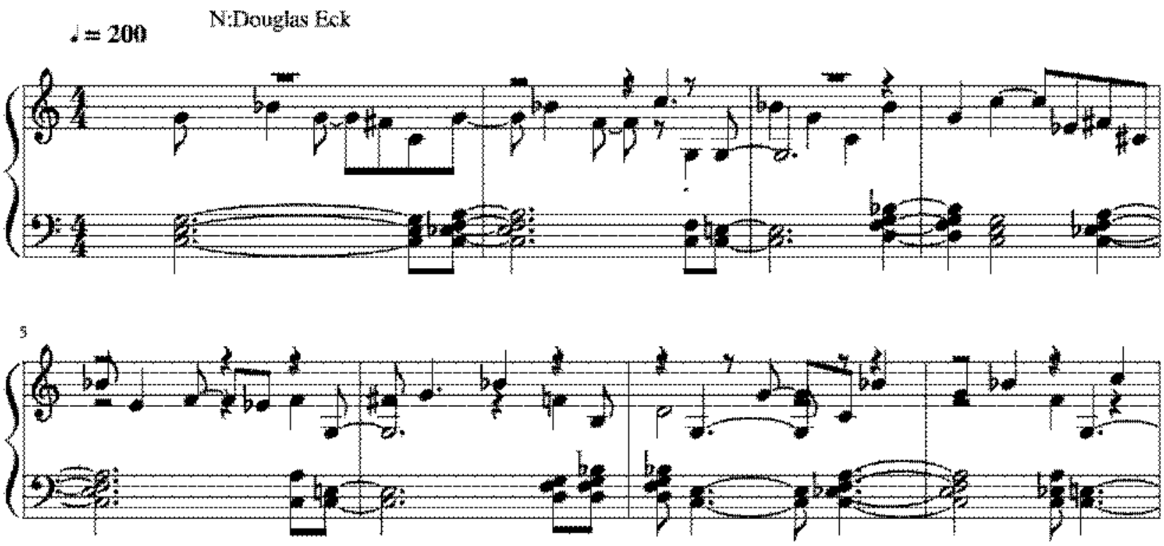
| Objective | Melody + Chords; Blues |
|---|---|
| Representation | Symbolic; One-hot2; Note end; Chord as note |
| Architecture | LSTM |
| Strategy | Iterative feedforward |
This second experiment is interesting in that it simultaneously generates melody and chords. Note that in this second architecture, recurrent connexions are asymmetric as the authors wanted to ensure the preponderant role of chords. Chord blocks have recurrent connexions to themselves but also to melody blocks, whereas melody blocks do not have recurrent connexions to chord blocks. This means that chord blocks will receive previous step information about chords and melody, whereas melody blocks cannot use previous step information about chords. This somewhat ad hoc configuration of the recurrent connexions in the architecture is a way to control the interaction between harmony and melody in a master-slave manner. The control of the interaction and consistency between melody and harmony is indeed an effective issue and it will be further addressed in Section 39 where we will analyze alternative approaches.
36 Content Variability
A limitation of the iterative feedforward strategy on an RNN, as illustrated by the blues generation experiment described in Section 35.1.2, is that generation is deterministic. Indeed, a neural network is deterministic232232 232 There are stochastic versions of artificial neural networks – an RBM is an example – but they are not mainstream.. As a consequence, feedforwarding the same input will always produce the same output. As the generation of the next note, the next next note, etc., is deterministic, the same seed note will lead to the same generated series of notes233233 233 The actual length of the melody generated depends on the number of iterations.. Moreover, as there are only 12 possible input values (the 12 pitch classes), there are only 12 possible melodies.
36.1 Sampling
Fortunately, as we will see, the usual solution is quite simple. The assumption is that the output representation of the melody is one-hot encoded. In other words, the output representation is of a piano roll type, the output activation layer is softmax and generation is modeled as a classification task. See an example in Figure 70, where represents the conditional probability for the element (note) xt at step to be a C given the previous elements x<t (the melody generated so far).
The default deterministic strategy consists in choosing the class (the note) with the highest probability, i.e. , that is A in Figure 70. We can then easily switch to a nondeterministic strategy, by sampling the output which corresponds (through the softmax function) to a probability distribution between possible notes. By sampling a note following the distribution generated234234 234 The chance of sampling a given class/note is its corresponding probability. In the example shown in Figure 70, A has around one chance in two of being selected and B one chance in four., we introduce stochasticity in the process and thus variability in the generation.

36.1.1 #1 Example: CONCERT Bach Melody Symbolic Music Generation System
CONCERT (an acronym for CONnectionist Composer of ERudite Tunes) developed by Mozer [139] in 1994, was actually one of the first systems for generating music based on recurrent networks (and before LSTM). It is aimed at generating melodies, possibly with some chord progression as an accompaniment.
The input and output representation includes three aspects of a note: pitch, duration and harmonic chord accompaniment. The representation of a pitch, named PHCCCH, is inspired by the psychological pitch representation space of Shepard [173], and is based on five dimensions, as illustrated in Figure 71.

The three main components are as follows:
- •
the pitch height (PH),
- •
the (modulo) chroma circle (CC) cartesian coordinates, and
- •
the (harmonic) circle of fifths (CH) cartesian coordinates.
The motivation is in having a more musically meaningful representation of the pitch by capturing the similarity of octaves and also the harmonic similarity between a note and its fifth. The proximity of two pitches is determined by computing the Euclidean distance between their PHCCCH representations, that distance being invariant under transposition. The encoding of the pitch height is through a scalar variable scaled to range from -9.798 for C1 to +9.798 for C5. The encoding of the chroma circle and of the circle of fifths is through a six binary value vector, for the reasons detailed in [139]. The resulting encoding includes 13 input variables, with some examples shown in Table 8. Note that a rest is encoded as a pitch with a unique code.
| Pitch | PH | CC | CH | ||||||||||
| C1 | -9.798 | +1 | +1 | +1 | -1 | -1 | -1 | -1 | -1 | -1 | +1 | +1 | +1 |
| F | -7.349 | -1 | -1 | -1 | +1 | +1 | +1 | +1 | +1 | +1 | -1 | -1 | -1 |
| G2 | -2.041 | -1 | -1 | -1 | -1 | +1 | +1 | -1 | -1 | -1 | -1 | +1 | +1 |
| C3 | 0 | +1 | +1 | +1 | -1 | -1 | -1 | -1 | -1 | -1 | +1 | +1 | +1 |
| D | 1.225 | +1 | +1 | +1 | +1 | +1 | +1 | +1 | +1 | +1 | +1 | +1 | +1 |
| E3 | 1.633 | -1 | +1 | +1 | +1 | +1 | +1 | +1 | -1 | -1 | -1 | -1 | -1 |
| A4 | 8.573 | -1 | -1 | -1 | -1 | -1 | -1 | -1 | -1 | -1 | -1 | -1 | -1 |
| C5 | 9.798 | +1 | +1 | +1 | -1 | -1 | -1 | -1 | -1 | -1 | +1 | +1 | +1 |
| Rest | 0 | +1 | -1 | +1 | -1 | +1 | -1 | +1 | -1 | +1 | -1 | +1 | -1 |
Durations are considered at a very fine-grain level, each beat (a quarter note) being divided into twelfths, thus having a duration of 12/12. This choice allows to represent binary (two or four divisions) as well as ternary (three divisions) rhythms. In a similar way to the representation of pitch, a duration is represented through a scalar and two circle coordinates, for 1/4 and 1/3 beat cycles, as illustrated in Figure 72, resulting in five dimensions directly encoded through a five binary value vector (see more details in [139]). The temporal scope is a note step, that is the granularity of processing by the architecture is a note235235 235 And not a fixed time step as for most of recurrent architectures, e.g., in Section 35.1.1. The various types of temporal scope have been introduced in Section 13.1..

Chords are represented in an extensional way as a triad or a tetrachord, through the root, the third (major or minor) and the fifth (perfect, augmented or diminished), with the possible addition of a seventh component (minor or major). To represent the next note to be predicted, the CONCERT system actually uses both this rich and distributed representation (named next-node-distributed, see Figure 73) and a more concise and traditional representation (named next-node-local), in order to be more intelligible. The activation function is the sigmoid function rescaled to the range and the cost function is mean squared error.

In the generation phase, the output is interpreted as a probability distribution over a set of possible notes as a basis for deciding the next note in a nondeterministic way, following the sampling strategy.
CONCERT has been tested on different examples, notably after training with melodies of J. S. Bach. Figure 74 shows an example of a melody generated based on the Bach training set. Although now a bit dated, CONCERT has been a pioneering model and the discussion in the article about representation issues is still relevant.
Note also that CONCERT (which is summarized in Table 9) is representative of the early generation systems, before the advent of deep learning architectures, when representations were designed with rich handcrafted features. One of the benefits of using deep learning architectures is that this kind of rich and deep representation may be automatically extracted and managed by the architecture.

| Objective | Melody + Chords |
|---|---|
| Representation | Symbolic; Harmonics; Harmony; Beat |
| Architecture | RNN |
| Strategy | Iterative feedforward; Sampling |
36.1.2 #2 Example: Celtic Melody Symbolic Music Generation System
Another representative example is the system by Sturm et al. to generate Celtic music melodies [179]. The architecture used is a recurrent network with three hidden layers, which we could notate236236 236 Note that, as explained in Section 22.2, we notate the number of hidden layers without considering the input layer. as LSTM3, with 512 LSTM cells in each layer.
The corpus comprises folk and Celtic monophonic melodies retrieved from a repository and discussion platform named The Session [99]. Pieces that were too short, too complex (with varying meters) or contained errors were filtered out, leaving a dataset of 23,636 melodies. All melodies are aligned (transposed) onto the single C key. One of the specificities is that the representation chosen is textual, namely the token-based folk-rnn notation, a transformation of the character-based ABC notation (see Section 12.3). The number of input and output nodes is equal to the number of tokens in the vocabulary (i.e. with a one-hot encoding), in practice equal to 137. The output of the network is a probability distribution over its vocabulary.
Training the recurrent network is done in an iterative way, as the network learns to predict the next item. Once trained, the generation is done iteratively by inputing a random token or a specific token (e.g., corresponding to a specific starting note), feedforwarding it to generate the output, sampling from this probability distribution, and recursively using the selected vocabulary element as a subsequent input, in order to produce a melody element by element.
The final step is to decode the folk-rnn representation generated into a MIDI format melody to be played. See in Figure 75 for an example of a melody generated. One may also see and listen to results on [178]. The results are very convincing, with melodies generated in a clear Celtic style. The system is summarized in Table 10.

As observed in [67]: ‘‘It is interesting to note that in this approach the bar lines and the repeat bar lines are given explicitly and are to be predicted as well. This can cause some issues, since there is no guarantee that the output sequence of tokens would represent a valid song in ABC format. There could be too many notes in one bar for example, but according to the authors, this rarely occurs. This would tend to show that such an architecture is able to learn to count.’’237237 237 On this issue, see also [60].
| Objective | Melody |
|---|---|
| Representation | Symbolic; Text; Token-based; One-hot |
| Architecture | LSTM3 |
| Strategy | Iterative feedforward; Sampling |
37 Expressiveness
One limitation of most existing systems is that they consider fixed dynamics (amplitude) for all notes as well as an exact quantization (a fixed tempo), which makes the music generated too mechanical, without expressiveness or nuance.
A natural approach resides in considering representations recorded from real performances and not simply scores, and therefore with musically grounded (by skilled human musicians) variations of tempo and of dynamics, as discussed in Section 15.
Note that an alternative approach is to automatically augment the generated music information (e.g., a standard MIDI piece) with slight transformations on the amplitude and/or the tempo. An example is the Cyber-João system [30], which performs bossa nova guitar accompaniment with expressiveness, through automatic retrieval238238 238 By a mixed use of production rules and case-based reasoning (CBR). and application of rhythmic patterns239239 239 These patterns have been manually extracted from a corpus of performances by the guitarist and singer João Gilberto, one of the inventors of the Bossa nova style. One could also consider automatic extraction, as, for example, in [32]..
As noted in Section 15.3, in the case of an audio representation, expressiveness is implicit to the representation. However, it is difficult240240 240 But not impossible to achieve, regarding recent achievements made on audio source separation through deep learning techniques, as has been pointed out in Section 15.3. to separately control the expressiveness (dynamics or tempo) of a single instrument or voice as the representation is global.
37.1 Example: Performance RNN Piano Polyphony Symbolic Music Generation System
In [174], Simon and Oore present their architecture and methodology named Performance RNN. It is an LSTM-based recurrent neural network architecture. One of the specificities is in the dataset characteristics, as the corpus is composed of recorded human performances, with records of exact timing as well as dynamics for each note played. The corpus used is the Yamaha e-Piano Competition dataset, whose participants MIDI performance records are made available to the public [210]. It captures more than 1,400 performances by skilled pianists. To create additional training examples, some time stretching (up to 5% faster or slower) as well as some transposition (up to a major third) is applied.
The representation is adapted to the objective. At first look, it resembles a piano roll with MIDI note numbers but it is actually a bit different. Each time slice is a multi-one-hot vector of the possible values for each of the following possible events:
- •
start of a new note – with 128 possible values (MIDI pitches),
- •
end of a note – with 128 possible values (MIDI pitches),
- •
time shift – with 100 possible values (from 10 miliseconds to 1 second), and
- •
dynamics -- with 32 possible values (128 MIDI velocities quantized into 32 bins241241 241 See the description of the binning transformation in Section 16.).
An example of a performance representation is shown in Figure 76.

Some control is made available to the user, referred to as the temperature, which controls the randomness of the generated events in the following way:
- •
a temperature of 1.0 uses the exact distribution predicted,
- •
a value smaller than 1.0 reduces the randomness and thus increases the repetition of patterns, and
- •
a larger value increases the randomness and decreases the repetition of patterns.
| Objective | Polyphony; Performance control |
|---|---|
| Representation | Symbolic; One-hot4; Time shift; Dynamics |
| Architecture | LSTM |
| Strategy | Iterative feedforward; Sampling |
38 RNN and Iterative Feedforward Revisited
As we saw in previous examples, the iterative feedforward strategy is based on the idea of the recurrent neural network (RNN) architecture to iteratively generate successive item of a sequence. It looks like a recurrent neural network architecture and the iterative feedforward strategy are strongly coupled. Indeed, almost all RNN-based systems use an iterative feedforward strategy and recursively reenter the output produced (next time step generated) into the input. But we will introduce in this section some exceptions.
38.1 #1 Example: Time-Windowed Melody Symbolic Music Generation System
The experiments by Todd in [190] were one of the very first attempts (in 1989) at exploring how to use artificial neural networks to generate music. Although the architectures he proposed are not directly used nowadays, his experiments and discussion were pioneering and are still an important source of information.
Todd’s objective was to generate a monophonic melody in some iterative way. He has experimented with different choices for representing the notes (see Section 10.3) and the durations, but finally had decided to use a conventional pitch note representation with a one-hot encoding and a time step temporal scope approach. The time step is set at the duration of an eighth note. In most of experiments, input melodies used for the training are 34 time steps long (that is, four measures and a half long), padded at the end with rests. A note begin is represented with a specific token and is encoded as an additional value encoding node (see Sections 14.1 and 16.7). Rests are not encoded explicitly but as the absence of a note, i.e. as the note one-hot encoding being all filled with null values (see Section 16.7).
The first experiment is what the author named Time-Windowed architecture, where a sliding window of successive time-periods of fixed size is considered. In practice this sliding window of a melody segment is one measure long, i.e. 8 time steps. Its representation may be considered as a piano roll, like in the MiniBach architecture (see Section 32.2), with the successive one-hot encodings of notes for the 8 successive time steps, notated as One-hot8.
The architecture is a feedforward network (and not an RNN), with a melody segment as its input, the next melody segment as its output and with a single hidden layer. Generation is conducted iteratively (and recursively), melody segment by melody segment. The architecture is illustrated in Figure 77.

For each time step of the melody segment, the predicted note is the one with the highest probability. Because of the zero-hot encoding of a rest (i.e. as all values being null), there is an ambiguity between the case of every possible note has a low probability and the case of a rest (see Section 16.7). For that reason, a probability threshold is introduced, namely 0.5. Thus, the predicted note is the one with the highest probability if it is greater than 0.5 and is a rest otherwise.
The network is trained in a supervised way by presenting a melody segment as an input and its corresponding next segment as the output, and repeating this for various segments. Note that, as the architecture is not recurrent, although the network will learn the pairwise correlations between two successive melody segments242242 242 In that respect, the Time-Windowed model is analog to an order 1 Markov model (considering only the previous state) at the level of a melody measure., there is no explicit memory for learning long term correlations such as in the case of a recurrent network architecture. Thus, although the author does not show a comparison with its next experiment (see next section), the architecture appears to have a low ability to learn long term correlations. The Time-Windowed architecture is summarized in Table 12.
| Objective | Melody |
|---|---|
| Representation | Symbolic; Piano roll; One-hot8; Note begin; Implicit rest |
| Architecture | Feedforward |
| Strategy | Iterative feedforward |
38.2 #2 Example: Sequential Melody Symbolic Music Generation System
In [190], Todd proposed another architecture, that he named Sequential, as notes are generated in a sequence. It is illustrated in Figure 78.
The input layer is divided in two parts, named the context and the plan. The context is the actual memory (of the melody generated so far) and consists in units corresponding to each note (D4 to C6), plus a unit about the note begin information (notated as “nb” in Figure 78). Therefore, it receives information from the output layer which produces next note, with a reentering connexion corresponding to each unit243243 243 Note that the output layer is isomorphic to the context layer.. In addition, as Todd explains it: ‘‘A memory of more than just the single previous output (note) is kept by having a self-feedback connection on each individual context unit.’’244244 244 This is a peculiar characteristic of this architecture, as in a standard recurrent network architecture recurrent connexions are encapsulated within the hidden layer (see Figures 46 and 50). The argument by Todd in [190] is that context units are more interpretable than hidden units: “Since the hidden units typically compute some complicated, often uninterpretable function of their inputs, the memory kept in the context units will likely also be uninterpretable. This is in contrast to [this] design, where, as described earlier, each context unit keeps a memory of its corresponding output unit, which is interpretable.”
The plan represents a melody (among many) that the network has learnt. Todd has experimented with various encodings, one-hot or distributed (through a many-hot embedding).

Training is done by selecting a plan (melody) to be learnt. The activations of the context units are initialized to 0 in order to begin with a clean empty context. The network is then feedforwarded and its output, corresponding to the first time step note, is compared to the first time step note of the melody to be learnt, resulting in adjustment of the weights. The output values245245 245 Actually, as an optimization, Todd proposes in the following of his description to pass back the target values and not the output values. are passed back to the current context. And then, the network is feedforwarded again, leading to the next time step note, again compared to the melody target, and so on until the last time step of the melody. This process is then repeated for various plans (melodies).
Generation of new melodies is conducted by feedforwarding the network with a new plan embedding, corresponding to a new melody (not part of the training plans/melodies). The activations of the context units are initialized to 0 in order to begin with a clean empty context. The generation takes place iteratively, time step after time step. Note that, as opposed to most cases of the iterative feedforward strategy (Section 35.1), in which the output is explicitly reentered (recursively) into the input of the architecture, in Todd’s Sequential architecture the reentrance is implicit because of the specific nature of the recurrent connexions: the output is reentered into the context units while the input – the plan melody – is constant.
After having trained the network on a plan melody, various melodies may be generated by extrapolation by inputing new plans, as shown in Figure 79. A repeat sign : indicates when the network output goes into a fixed loop.
o) 
e1) 
e2) 
One could also do interpolation between several (two or more) plans melodies that have been learnt246246 246 Note that this way of doing is actually some precursor of doing interpolation on embeddings of melodies to be generated by combining a decoder feedforward strategy and an iterative feedforward strategy, such as for example in the VRAE or the MusicVAE systems, to be described in Sections 40.2.3 and 42.1, respectively.. Examples are shown in Figure 80. The Sequential architecture is summarized in Table 13.
oA)
oB) 
i1) 
i2) 
| Objective | Melody |
|---|---|
| Representation | Symbolic; Piano roll; One-hot; Note begin; Implicit rest |
| Architecture | RNN |
| Strategy | Iterative feedforward |
38.3 #3 Example: BLSTM Chord Accompaniment Symbolic Music Generation System
The BLSTM (Bidirectional LSTM) chord accompaniment system by Lim et al. [120] is a rare and interesting case247247 247 As noted in Sections 25.2 and 35.1. of an accompaniment system based on a recurrent architecture. The objective is to generate a progression (sequence) of chords as an accompaniment to a melody (specified symbolically).
The corpus is imported from a now defunct lead sheet public data base. The authors selected 2,252 selected lead sheets of various western modern music (rock, pop, country, jazz, folk, R&B, children’s song, etc.), all in major key and the majority with a single chord per measure (otherwise only the first chord is considered). This results in a training set of 1,802 songs (making a total of 72,418 measures) and a test set of 450 songs (17,768 measures). All songs are transposed (aligned) to C major key.
Desired characteristics are extracted from the original XML files and converted to a CSV248248 248 CSV stands for Comma-separated values. (spreadsheet) matrix format, as shown in Figure 81. The specificities (simplifications) of the representation are as follows:
- •
for the melody249249 249 And obviously also for the chords., only pitch classes are considered (and octaves are not), resulting in a 12 notes one-hot encoding (named 12-semitone-vector) plus the rest; and
- •
for the chords, only their primary triads are considered, with only two types: major and minor, resulting in a 24 chords one-hot encoding.

The architecture is a bidirectional LSTM with two LSTM layers, each one with 128 units. The motivation is to provide the network with the musical context backward and also forward in time. The time step considered by the architecture is four measures long, as shown in Figure 82. The tanh function is used as the non linear activation function for the hidden layers and softmax is used as the output layer activation function, with categorical cross-entropy as its associated cost function.

Training is done with various four measures long samples as input and their associated four chords as output, generated by sliding a four measures long window over each training song. Generation is done by iteratively feedforwarding successive four measures long melody fragments (time slices) of a song and concatenating the resulting four measures long chord progression fragments.
The architecture is peculiar in that, although recurrent, generation is not recursive and the output data has a different nature and structure (chords) than the input data (notes). Furthermore, note that, although the strategy is iterative and the architecture is recurrent, the granularity of each iterative step is quite coarse as it is 4 measures long, as opposed to most of systems based on recurrent architectures and iterative feedforward strategy which consider the time step at the level of the smallest notre duration (see, e.g., the system analyzed in Section 35.1.1). This kind of mixed architecture/strategy between forward/single step and recurrent/iterative may have been motivated by the objective of capturing sufficiently the history of horizontal correlations (between notes of the melody and between chords of the accompaniment) as the LSTM cells focus on capturing the history of vertical correlations (between notes and chords).
The system has been evaluated by comparing to some hidden Markov model (HMM) model and to some deep neural network–HMM hybrid model (named DNN-HMM, see details in [199]), both quantitatively (by comparing the accuracies and through confusion matrixes), and qualitatively (through a web-based survey of 25 musically untrained participants). Results are showing a better accuracy and preference for the BLSTM model, see a simple example in Figure 83. The authors note that the evaluation also shows that, when songs are unknown, the preference for the BLSTM model is weaker. They conjecture that this is because BLSTM often generates a more diverse chord sequence than the original. The BLSTM system is summarized in Table 14.

| Objective | Accompaniment; Chord sequence; Western modern music |
|---|---|
| Representation | Symbolic; CSV; One-hot(12* + 244); Rest |
| Architecture | LSTM2 |
| Strategy | Iterative feedforward |
38.4 Summary
In summary, we have seen that an RNN architecture is usually coupled to an iterative feedforward strategy, which allows a recursive seed-based variable length generation, as discussed in Section 35. However, there are some exceptions:
- •
the Time-Windowed system by Todd (Section 38.1) uses an iterative feedforward strategy on a feedforward architecture in order to generate a melody, and
- •
the BLSTM system (Section 38.3) uses an iterative feedforward strategy on a recurrent architecture in order to generate a chord accompaniment to a melody.
We will see further (with the VRAE system to be described in Section 40.2.3) the use of an RNN Encoder-Decoder compound architecture (Section 30.3), as a way to decouple the length of the input sequence with the length of the output sequence, by combining the decoder feedforward strategy with the iterative feedforward strategy.
Some other examples of couplings between architectures and strategies, or between challenges, will be discussed in Section 48. Before that, we will continue to analyze challenges and possible solutions or directions.
39 Melody-Harmony Interaction
When the objective is to generate simultaneously a melody with an accompaniment, expressed through some harmony or counterpoint250250 250 Harmony and counterpoint are dual approaches of accompaniment with different focus and priorities. Harmony focuses on the vertical relations between simultaneous notes, as objects on their own (chords), and then considers the horizontal relations between them (e.g., harmonic cadences). Conversely, counterpoint focuses on the horizontal relations between successive notes for each simultaneous melody (a voice), and then considers the vertical relations between their progression (e.g., to avoid parallel fifths). Note that, although their perspectives are different, the analysis and control of relations between vertical and horizontal dimensions are their shared objectives., an issue is the musical consistency between the melody and the harmony. Although a general architecture such as MiniBach (Section 32.2) is supposed to have learnt correlations, interactions between vertical and horizontal dimensions are not explicitly considered.
We have analyzed in Section 35.1.2 an example of a specific architecture to generate simultaneously melody and chords, with explicit relations between them (i.e. chords can use previous step information about melody but not the opposite). However, this architecture is a bit ad hoc. In the following sections, we will analyze some more general architectures having in mind interactions between melody and harmony.
39.1 #1 Example: RNN-RBM Polyphony Symbolic Music Generation System
In [11], Boulanger-Lewandowski et al. have associated to the RBM-based architecture introduced in Section 34.2.3 a recurrent network (RNN) in order to represent the temporal sequence of notes. The idea is to couple the RBM to a deterministic RNN with a single hidden layer, such that
- •
the RNN models the temporal sequence to produce successive outputs, corresponding to successive time steps,
- •
which are parameters, more precisely the biases, of an RBM that models the conditional probability distribution of the accompaniment notes, i.e. which notes should be played together.
In other words, the objective is to combine a horizontal view (temporal sequence) and a vertical view (combination of notes for a particular time step). The resulting architecture named RNN-RBM is shown in Figure 84, and can be interpreted as follows:

- •
the bottom line represents the temporal sequence of RNN hidden units u(0), u(1), …, u(t), where u(t) notation means251251 251 Note that the usual notation would be ut, as the u(t) notation is usually reserved to index dataset examples (th example), see Section 25. the value of the RNN hidden layer u at time (index) ; and
- •
the upper part represents the sequence of each RBM instance at time , which we could notate RBM(t), with
- –
v(t) its visible layer with its bias,
- –
h(t) its hidden layer with its bias, and
- –
the weight matrix of connexions between the visible layer v(t) and the hidden layer h(t).
- –
There is a specific training algorithm, which we will not detail here, please refer to [11]. During generation, each time step of processing is as follows:
- •
- •
sample from RBM(t) by using block Gibbs sampling to produce v(t), and
- •
feedforward the RNN with v(t) as the input, using the RNN hidden layer value u(t-1), in order to produce the RNN new hidden layer value u(t) via Equation 33, where
- –
is the weight matrix and the bias for the connexions between the input layer of the RBM and the hidden layer of the RNN; and
- –
is the weight matrix for the recurrent connexions of the hidden layer of the RNN.
- –
| (31) |
| (32) |
| (33) |
Note that the biases and of RBM(t) are variable for each time step, in other words they are time dependent, whereas the weight matrix for the connexions between the visible and the hidden layer of RBM(t) is shared for all time steps (for all RBMs), i.e. it is time independent252252 252 , , and weight matrices are also shared and thus time independent..
Four different corpora have been used in the experiments: classical piano, folk tunes, orchestral classical music and J. S. Bach chorales. Polyphony varies from 0 to 15 simultaneous notes, with an average value of 3.9. A piano roll representation is used with many-hot encoding of 88 units representing pitches from A0 to C8. Discretization (time step) is a quarter note. All examples are aligned onto a single common tonality: C major or minor. An example of a sample generated in a piano roll representation is shown in Figure 85. The quality of the model has made RNN-RBM, summarized at Table 15, one of the reference architectures for polyphonic music generation.

| Objective | Polyphony |
|---|---|
| Representation | Symbolic; Many-hot |
| Architecture | RBM-RNN |
| Strategy | Iterative feedforward; Sampling |
39.1.1 Other RNN-RBM Systems
There have been a few systems following on and extending the RNN-RBM architecture, but they are not significantly different and furthermore they have not been thoroughly evaluated. However, it is worth mentioning the following:
39.2 #2 Example: Hexahedria Polyphony Symbolic Music Generation Architecture
The system for polyphonic music proposed by Johnson in his Hexahedria blog [94] is hybrid and original in that it integrates into the same architecture
- •
a first part made of two RNNs (actually LSTM) layers, each with 300 hidden units, recurrent over the time dimension, which are in charge of the temporal horizontal aspect, that is the relations between notes in a sequence. Each layer has connections across time steps, while being independent across notes; and
- •
a second part made of two other RNN (LSTM) layers, with 100 and 50 hidden units, recurrent over the note dimension, which are in charge of the harmony vertical aspect, that is the relations between simultaneous notes within the same time step. Each layer is independent between time steps but has transversal directed connexions between notes.
We can notate this architecture as LSTM2+2 in order to highlight the two successive 2-level recurrent layers, recurrent in two different dimensions (time and note). The architecture is actually a kind of integration within a single architecture254254 254 We will see in Section 39.3 an alternative architecture, named Bi-Axial LSTM, where each of the 2-level time-recurrent layers is encapsulated into a different architectural module. of the RNN-RBM architecture described in previous section. The main originality is in using recurrent networks not only on the time dimension but also on the note dimension, more precisely on the pitch class dimension. This latter type of recurrence is used to model the occurence of a simultaneous note based on other simultaneous notes. Like for the time relation, which is oriented towards the future, the pitch class relation is oriented towards higher pitch, from C to B.


The resulting architecture is shown in its folded form in Figure 86 and in its unfolded form255255 255 Our unfolded pictorial representation of an RNN shown in Figure 45 was actually inspired by Johnson’s Hexahedria pictorial representation. in Figure 87, with three axes represented:
- •
the flow axis, shown horizontally and directed from left to right, represents the flow of (feedforward) computation through the architecture, from the input layer to the output layer;
- •
the note axis, shown vertically and directed from top to bottom, represents the connexions between units corresponding to successive notes of each of the two last (note-oriented) recurrent hidden layers; and
- •
the time axis, only in the unfolded Figure 87, shown diagonally and directed from top left to bottom right, represents the time steps and the propagation of the memory within a same unit of the two first (time-oriented) recurrent hidden layers.
The dataset is constructed by extracting 8 measures long parts from MIDI files from the Classical piano MIDI database [105]. The input representation used is piano roll, with the pitch represented as the MIDI note number. More specific information is added: the pitch class, the previous note played (as a way to represent a possible hold), how many times a pitch class has been played in the previous time step and the beat (the position within the measure, assuming a 4/4 time signature). The output representation is also a piano roll, in order to represent the possibility of more than one note at the same time. Generation is done in an iterative way (i.e. following the iterative feedforward strategy), as for most recurrent networks. The system is summarized in Table 16.
| Objective | Polyphony |
|---|---|
| Representation | Symbolic; Piano roll; Hold; Beat |
| Architecture | LSTM2+2 |
| Strategy | Iterative feedforward; Sampling |
39.3 #3 Example: Bi-Axial LSTM Polyphony Symbolic Music Generation Architecture
Johnson recently proposed an evolution of his original Hexahedria architecture, described in Section 39.2, named Bi-Axial LSTM (or BALSTM) [95].
The representation used is piano roll, with note hold and rest tokens added to the vocabulary. Various corpora are used: the JSB Chorales dataset, a corpus of 382 four-part chorales by J. S. Bach [1]; the MuseData library, an electronic classical music library from CCARH in Stanford [77]; the Nottingham database, a collection of 1,200 folk tunes in ABC notation [54]; and the Classical piano MIDI database [105]. Each dataset is transposed (aligned) into the key of C major or C minor.
The probability of playing a note depends on two types of information:
- •
all notes at previous time steps – this is modeled by the time-axis module; and
- •
all notes within the current time step that have already been generated (the order being lowest to highest) – this is modeled by the note-axis module.
There is an additional front end layer, named ‘‘Note Octaves’’, which transforms each note into a vector of all its possible corresponding octave notes (i.e. an extensional version of pitch classes). The resulting architecture is illustrated in Figure 88256256 256 This figure comes from the description of another system based on the Bi-Axial LSTM architecture, named DeepJ, which will be described in Section 40.3.4.. The “x2” represents the fact that each module is stacked twice (i.e. has two layers).
The time-axis module is recurrent in time (as for a classical RNN), the LSTM weights being shared across notes in order to gain note transposition invariance. The note-axis module257257 257 Note that, as opposed to Johnson’s first architecture (that we refer to as Hexahedria, and which has been introduced in Section 39.2), which integrates the 2-level time-recurrent layers with the 2-level note-recurrent layers within a single architecture and therefore notated as LSTM2+2, the Bi-Axial LSTM architecture explicitly separates each 2-level time-recurrent layers into distinct architectural modules and is therefore notated as LSTM2. is recurrent in note. For each note input of the note-axis module, represents the concatenation of the corresponding output from the time-axis module with the already predicted lower notes. Sampling (into a binary value, by using a coin flip) is applied to each note output probability in order to compute the final prediction (whether that note is played or not).

As pointed out by Johnson [95], during the training phase, as all the notes at all time steps are known, the training process may be accelerated by processing each layer independently (e.g., on a GPU), by running input through the two time-axis layers in parallel across all notes, and using the two note-axis layers to compute probabilities in parallel across all time steps.
The generation phase is sequential for each time step (by following both the iterative feedforward strategy and the sampling strategy). An excerpt of music generated is shown in Figure 89.
The Bi-Axial LSTM system, summarized in Table 17, has been evaluated and compared to some other architectures. The author reports noticeably better results with Bi-Axial LSTM, the greatest improvements being on the MuseData [77] and the Classical piano MIDI database [105] datasets, and states in [95] that: ‘‘It is likely due to the fact that those datasets contain many more complex musical structures in different keys, which are an ideal case for a translation-invariant architecture.’’ Note that an extension of the Bi-Axial LSTM architecture with conditioning, named DeepJ, will be introduced in Section 40.3.4.

| Objective | Polyphony |
|---|---|
| Representation | Symbolic; Piano roll; Hold; Rest |
| Architecture | Bi-Axial LSTM = LSTM2 |
| Strategy | Iterative feedforward; Sampling |
40 Control
A deep architecture generates musical content matching the style learnt from the corpus. This capacity of induction from a corpus without any explicit modeling or programming is an important ability, as discussed in Chapter id1 and also in [52]. However, like a fast car that needs a good steering wheel, control is also needed as musicians usually want to adapt ideas and patterns borrowed from other contexts to their own objective and context, e.g., transposition to another key, minimizing the number of notes, finishing with a given note, etc.
40.1 Dimensions of Control Strategies
Arbitrary control is a difficult issue for deep learning architectures and techniques because neural networks have not been designed to be controlled. In the case of Markov chains, they have an operational model on which one can attach constraints to control the generation258258 258 Two examples are Markov constraints [149] and factor graphs [148].. However, neural networks do not offer such an operational entry point and the distributed nature of their representation does not provide a clear relation to the structure of the content generated. Therefore, as we will see, most of strategies for controlling deep learning generation rely on external intervention at various entry points (hooks) and levels:
- •
input,
- •
output,
- •
input and output, and
- •
encapsulation/reformulation.
Various control strategies can be employed:
- •
sampling,
- •
conditioning,
- •
input manipulation,
- •
reinforcement, and
- •
unit selection.
We will also see that some strategies (such as sampling, see Section 40.2) are more bottom-up and others (such as structure imposition, see Section 40.5.1, or unit selection, see Section 40.7) are more top-down. Lastly, there is also a continuum between partial solutions (such as conditioning/parametrization, see Section 40.3) and more general approaches (such as reinforcement, see Section 40.6).
40.2 Sampling
Sampling from a stochastic architecture (such as a restricted Boltzmann machine (RBM), see Section 34.2), or from a deterministic architecture (in order to introduce variability, see Section 36.1), may be an entry point for control if we introduce constraints into the sampling process. This is called constrained sampling, see for example the C-RBM system in Section 40.5.1.
Constrained sampling is usually implemented by a generate-and-test approach, where valid solutions are picked from a set of random samples generated from the model. But this could be a very costly process and, moreover, with no guarantee of success. A key and difficult issue is therefore how to guide the sampling process in order to fulfill the constraints.
40.2.1 Sampling for Iterative Feedforward Generation
In the case of an iterative feedforward strategy on a recurrent network, some refinements in the sampling procedure can be made.
In Section 36.1, we introduced the technique of sampling the softmax output of a recurrent network in order to introduce content variability. However, this may sometimes lead to the generation of an unlikely note (with a low probability). Moreover, as noted in [67], generating such a “wrong” note can have a cascading effect on the remaining of the generated sequence.
A counter measure consist in adjusting a learnt RNN model (conditional probability distribution , as defined in Section 25) by not considering notes with a probability under a certain threshold. The new model, with a probability distribution , is defined in Equation 34 following [204], where:
| (34) |
- •
is the note maximum probability,
- •
is the threshold hyperparameter, and
- •
is a normalization constant.
A slightly more sophisticated version interpolates between the original distribution and the deterministic variant259259 259 See Section 36.1., with some temperature user control hyperparameter (see more details in (67, Section 4.1.1.3)).
This technique will be further generalized and combined with the conditioning strategy in order to control the generation of notes at specific positions via positional constraints. This will be exemplified by the Anticipation-RNN system to be introduced in Section 40.3.5.
40.2.2 Sampling for Incremental Generation
In the case of an incremental generation (to be introduced in Section 44), the user may select
- •
on which part (e.g., a given part of a melody and/or a given voice) sampling will occur (or reoccur), and
- •
the interval of possible values on which sampling will occur.
In the case of the DeepBach system (to be introduced in Section 45.2), this will be the basis for introducing user control on the generation, notably to regenerate only some parts of a music, to restrict note range, and to impose some basic rhythm.
40.2.3 Sampling for Variational Decoder Feedforward Generation
Another interesting case is the use of sampling for generative models, such as variational autoencoders (VAEs) and generative adversarial networks (GANs), to be introduced in Section 40.2.4. We will see that some nice control of the sampling, e.g., to produce an interpolation, averaging or attribute modification, will produce meaningful variations in the content generated by the decoder feedforward strategy. Moreover, as has been discussed in Section 23.2, a variational autoencoder (VAE) is interesting for its ability for controlling generation over significant dimensions that have been learnt.
#1 Example: VRAE Video Game Melody Symbolic Music Generation System
In [50], Fabius and van Amersfoort propose the extension of the RNN Encoder-Decoder architecture to the case of a variational autoencoder (VAE), which is therefore named a variational recurrent autoencoder (VRAE). Both the encoder and the decoder encapsulate an RNN (actually an LSTM), as has been explained in Section 30.3. In terms of strategy, the VRAE combines the iterative feedforward strategy with the decoder feedforward strategy and the sampling strategy.
The corpus used in the experiment is a set of MIDI files of eight video game songs from the 1980s and 1990s (Sponge Bob, Super Mario, Tetris…), which are divided into various shorter parts of 50 time steps. A one-hot encoding of 49 possible pitches is used (pitches with too few occurrences of notes were not considered). Experiments have been conducted with 2 or 20 hidden layer units (latent variables). Training takes place as for training recurrent networks, i.e. for each input note presenting the next note as the output.
After the training phase, the latent space vector can be sampled and used by the RNN encapsulated within the decoder to generate iteratively a melody. This could be done by random sampling or also by interpolating between the values of the latent variables corresponding to different songs that have been learnt, creating a sort of “medley” of these songs. Figure 90 visualizes the organisation of the encoded data in the latent space, each color representing the data points from one song. The result is positive, but the low musical quality of the corpus hampers a careful evaluation. The VRAE system is summarized in Table 18.

| Objective | Melody; Video game songs |
|---|---|
| Representation | Symbolic; MIDI; One-hot |
| Architecture | Variational(Autoencoder(LSTM, LSTM)) |
| Strategy | Decoder feedforward; Iterative feedforward; Sampling |
#2 Example: GLSR-VAE Melody Symbolic Music Generation System
The architecture proposed by Hadjeres and Nielsen in [69] is based on a variational autoencoder (VAE) architecture (Section 23.2), but it proposes an improvement in the control of the variation in the generation, named geodesic latent space regularization (GLSR), with a system named GLSR-VAE.
The starting point is that a straight line between two points in the latent space will not necessarily produce the best interpolation in the generated content domain space. The idea is to introduce a regularization to relate variations in the latent space to variations in the attributes of the decoded elements. The details of the definition of the added cost term may be found in [69].
The experiment consists in generating chorale melodies in the style of J. S. Bach. The dataset comprises monophonic soprano voices from the J. S. Bach chorales corpus [5].
GLSR-VAE shares the principles of representation initiated by the DeepBach system (Section 44.2), that is
- •
one-hot encoding of a note,
- •
with the addition to the vocabulary of the hold symbol ‘‘__’’ and the rest symbol to specify, respectively, a note repetition and a rest (see Section 16.7), and
- •
using the names of the notes (with no enharmony, e.g., F and G are considered to be different, see Section 14.2).
Quantization is at the level of a sixteenth note. The latent variable space is set to 12 dimensions (12 latent variables).
In the experiments conducted, regularization is executed on a first dimension which has been found260260 260 See Section 23.2. to represent the number of notes (named z1). Figure 91 shows the organisation of the encoded data in the latent space, with the number of notes z1 being the abscissa axis, with from left to right an effective progressive increase in the number of notes (shown with scales of colors). Figure 92 shows examples of the melodies generated (each 2 measures long, separated by double bar lines) while increasing z1, showing a progressive correlated densification of the melodies generated.


GLSR-VAE is summarized in Table 19. More examples of sampling from variational autoencoders will be described in Section 42.1.
| Objective | Melody; Bach |
|---|---|
| Representation | Symbolic; Piano roll; One-hot; Hold; Rest; Fermata; No enharmony |
| Architecture | Variational(Autoencoder(LSTM, LSTM)); Geodesic regularization |
| Strategy | Decoder feedforward; Sampling |
40.2.4 Sampling for Adversarial Generation
Another example of a generative model is a generative adversarial networks (GAN) architecture. In such an architecture, after having trained the generator in an adversarial way, generation of content is done by sampling latent random variables.
Example: Mogren’s C-RNN-GAN Classical Polyphony Symbolic Music Generation System
The objective of Mogren’s C-RNN-GAN [135] system is the generation of single voice polyphonic music. The representation chosen is inspired by MIDI and models each musical event (note) via four attributes: duration, pitch, intensity and time elapsed since the previous event, each attribute being encoded as a real value scalar. This allows the representation of simultaneous notes (in practice up to three). The musical genre of the corpus is classical music, retrieved in MIDI format from the Web and contains 3,697 pieces from 160 composers.
C-RNN-GAN is based on a generative adversarial networks (GAN) architecture, with both the generator and the discriminator being recurrent networks261261 261 This generative GAN architecture encapsulates two recurrent networks, in the same spirit that the generative VRAE variational autoencoder architecture encapsulates two recurrent networks as explained in Section 40.2.3., more precisely each having two LSTM layers with 350 units each. A specificity is that the discriminator (but not the generator) has a bidirectional recurrent architecture, in order to take context from both the past and the future for its decisions. The architecture is shown in Figure 93 and summarized in Table 20.

The discriminator is trained, in parallel to the generator, to classify if a sequence input is coming from the real data. Similar to the case of the encoder part of the RNN Encoder-Decoder, which summarizes a musical sequence into the values of the hidden layer (see Section 30.3), the bidirectional RNN decoder part of the C-RNN-GAN summarizes the sequence input into the values of the two hidden layers (forward sequence and backward sequence) and then classifies them.
An example of generated music is shown in Figure 94. The author conducted a number of measurements on the generated music. He states that the model trained with feature matching262262 262 A regularization technique for improving GANs, see Section 28.1. achieves a better trade-off between structure and surprise than the other variants. Note that this is consonant with the use of the feature matching regularization technique to control creativity in MidiNet (to be introduced in Section 40.3.3). C-RNN-GAN is summarized in Table 20.

| Objective | Polyphony |
|---|---|
| Representation | Symbolic; MIDI; Value encoding4 |
| Architecture | GAN(Bidirectional-LSTM2, LSTM2) |
| Strategy | Iterative feedforward; Sampling263263 263 Note that we do not consider GAN (adversarial) as a strategy, because we consider that the essence of GAN is about the architecture and the strategy about the training phase, whereas we are here concerned with the strategy about the generation phase. After having trained the generator, generation uses a conventional iterative feedforward strategy for an RNN with the addition of some sampling for the variability, as described in Section 36.1. |
40.2.5 Sampling for Other Generation Strategies
Sampling may also be combined with other strategies for content generation, as for instance
40.3 Conditioning
The idea of conditioning (sometimes also named conditional architecture) is to condition the architecture on some extra information, which could be arbitrary, e.g., a class label or data from other modalities. Examples are
- •
a bass line or a beat structure, in the rhythm generation architecture (Section 40.3.1),
- •
a chord progression, in the MidiNet architecture (Section 40.3.3),
- •
the previously generated note, in the VRASH architecture (Section 40.3.6),
- •
some positional constraints on notes, in the Anticipation-RNN architecture (Section 40.3.5),
- •
a musical genre or an instrument, in the WaveNet architecture (Section 40.3.2), and
- •
a musical style, in the DeepJ architecture (Section 40.3.4).
In practice, the conditioning information is usually fed into the architecture as an additional input layer (for example, see Figure 54). This distinction between standard input and conditioning input follows a good architectural modularity principle264264 264 Note that we do not consider conditioning as a strategy because we consider that the essence of conditioning relates to the conditioning architecture. Generation uses a conventional strategy (e.g., single-step feedforward, iterative feedforward…) depending on the type of the architecture (e.g., feedforward, recurrent…).. Conditioning is a way to have some degree of parametrized control over the generation process.
The conditioning layer could be
- •
a simple input layer. An example is a tag specifying a musical genre or an instrument in the WaveNet system (Section 40.3.2),
- •
some output of some architecture, being
- –
the same architecture, as a way to condition the architecture on some history265265 265 This is close in spirit to a recurrent architecture (RNN). -- an example is the MidiNet system (Section 40.3.3) in which history information from previous measure(s) is injected back into the architecture, or
- –
another architecture – examples are the rhythm generation system (Section 40.3.1) in which a feedforward network in charge of the bass line and the metrical structure information produces the conditioning input, and the DeepJ system (Section 40.3.4) in which two successive transformation layers of a style tag produce an embedding used as the conditioning input.
- –
If the architecture is time-invariant – i.e. recurrent or convolutional over time –, there are two options
- •
global conditioning -- if the conditioning input is shared for all time steps, or
- •
local conditioning – if the conditioning input is specific to each time step.
The WaveNet architecture, which is convolutional over time (see Section 26.5), offers the two options, as will be analyzed in Section 40.3.2.
40.3.1 #1 Example: Rhythm Symbolic Music Generation System
The system proposed by Makris et al. [123] is specific in that it is dedicated to the generation of sequences of rhythm. Another specificity is the possibility to condition the generation relative to some particular information, such as a given beat or bass line.
The corpus includes 45 drum and bass patterns, each 16 measures long in 4/4 time signature, from three different rock bands and converted to MIDI. The representation of drums is described in Section 16.8 and summarized as follows. Different drum components (kick, snare, toms, hi-hat, cymbals) are considered as distinct simultaneous voices, following a many-hot approach, and encoded in text as a binary word of length 5, e.g., represents the simultaneous playing of kick and high-hat.
The representation also includes a condensed representation of the bass line part. It captures the voice leading perspective of the bass266266 266 The voice leading of the bass has proven a valuable aspect in harmonization systems, see, e.g., [72]., by specifying the pitch difference direction for the bass between two successive time steps. This is represented in a binary word of length 4, the first digit specifying the existence of a bass event () or a rest event (), while the three remaining digits specify the 3 possible directions for voice leading: steady (), upward () and downward (). Last, the representation includes some additional information representing the metrical structure (the beat structure), also through binary words. See further details in [123].
The architecture is a combination of a recurrent network (more precisely, an LSTM) and a feedforward network, representing the conditioning layer. The LSTM (two stacked LSTM layers with 128 or 512 units) is in charge of the drums part, while the feedforward network is in charge of the bass line and the metrical structure information. The outputs of these two networks are then merged267267 267 Note that in this system, the conditioning layer is added to the main architecture at its output level and not at its input level. Therefore an additional feedforward merge layer is introduced. We could notate the resulting architecture as Conditioning(Feedforward(LSTM2), Feedforward)., resulting in the architecture illustrated in Figure 95. The authors report that the conditioning layer (bass line and beat information) improves the quality of the learning and of the generation. It may also be used in order to mildly influence the generation. More details may be found in the article [123]. The architecture is summarized in Table 21.
An example of a rhythm pattern generated is shown in Figure 96 with in Figure 97 the use of a specific and more complex bass line as a conditioning input which produces a rhythm more elaborate. The piano roll like visual representation shows in its five successive lines (downwards) the kick, snare, toms, hi-hat and cymbals components events.


| Objective | Multivoice; Rhythm; Drums |
|---|---|
| Representation | Symbolic; Beat; Drums; Many-hot; Bass line; Note; Rest; Hold |
| Architecture | Conditioning(Feedforward(LSTM2), Feedforward) |
| Strategy | Iterative feedforward; Sampling |
40.3.2 #2 Example: WaveNet Speech and Music Audio Generation System
WaveNet, by van der Oord et al. [194], is a system for generating raw audio waveforms, quite innovative in that respect. It has been tested in three audio domains: multi-speaker, text-to-speech (TTS) and music.
The architecture is based on a convolutional feedforward network with no pooling layer. Convolutions are constrained in order to ensure that the prediction only depends on previous time steps, and are therefore named causal convolutions. The actual implementation is optimized through the use of dilated convolution (also called ‘‘à trous’’), where the convolution filter is applied over an area larger than its length by skipping input values with a certain step. Incrementally dilated successive convolution layers268268 268 The dilation is doubled for every layer up to a limit and then repeated, e.g., 1, 2, 4, …, 512, 1, 2, 4, …, 512, … enable networks to have very large receptive fields with just a few layers while preserving the input resolution throughout the network as well as computational efficiency (see [194] for more details). The architecture is illustrated in Figure 98.
Another specificity of WaveNet is in the training/generation asymmetry: during the training phase, predictions for all time steps can be made in parallel, whereas during the generation phase, predictions are sequential (following the iterative feedforward strategy).
The WaveNet architecture is made conditioning, as a way to guide the generation, by adding an additional tag as a conditioning input. We could thus notate the architecture as Conditioning(Convolutional(Feedforward), Tag).
There are actually two options:
- •
global conditioning, if the conditioning input is shared for all time steps; and
- •
local conditioning, if the conditioning input is specific to each time step.
An example of conditioning for a text-to-speech application domain is to feed in linguistic features from different speakers, e.g., North American or Mandarin Chinese English speakers, in order to generate speech with a specific prosody.

The authors also conducted preliminary work on conditioning models to generate music given a set of tags specifying, for example, genre or instruments. They state (without further details) that their preliminary attempt is promising [194]. WaveNet is summarized in Table 22.
Last, let us mention, a recent proposal as an offspring from WaveNet, which uses a symbolic representation (associated to the audio input) as the conditioning model/input, in order to better guide and structure the generation of (audio) music (see details in [126]).
| Objective | Audio |
|---|---|
| Representation | Audio; Waveform |
| Architecture | Conditioning(Convolutional(Feedforward), Tag); Dilated convolutions |
| Strategy | Iterative feedforward; Sampling |
40.3.3 #3 Example: MidiNet Pop Music Melody Symbolic Music Generation System
In [212], Yang et al. propose the MidiNet architecture, which is both adversarial and convolutional, for the generation of single or multitrack pop music monophonic melodies.
The corpus used is a collection of 1,022 pop music songs from the TheoryTab269269 269 Tabs are piano roll-like leadsheets, including melody, lyrics and notation of chords. online database [85] that provides two channels per tab, one for the melody and the other for the underlying chord progression. This allows two versions of the system: one with only the melody channel and another that additionally uses chords to condition melody generation. After all the preprocessing steps, the dataset is composed of 526 MIDI tabs (representing 4,208 measures). Data augmentation is then performed by circularly shifting all melodies and chords to any of the 12 keys, leading to a final dataset of 50,496 measures of melody and chord pairs for training.
The representation is obtained by transforming each channel of MIDI files into a one-hot encoding of 8 measures long piano roll representations, using one of the encodings to represent silence (rest) and neglecting the velocity of the note events. The time step is set at the smallest note, a sixteenth note. All melodies have been transposed in order to fit within the two-octave interval C B270270 270 However, the authors considered all the 128 MIDI note numbers (corresponding to the C G interval) in a one-hot encoding and state in [212] that: “In doing so, we can detect model collapsing more easily, by checking whether the model generates notes outside these octaves.”. Note that the current representation does not distinguish between a long note and two short repeating notes, and the authors mention considering future extensions in order to emphasize the note onsets.
For chords, instead of using a many-hot vector extensional representation of dimension 24 (for the two octaves), the authors state that they found it more efficient to use an intensional representation of dimension 13: 12 for the pitch-class (key) and 1 for the chord type (major or minor).
The architecture271271 271 The architecture is complex, please see further details in [212]. is illustrated in Figures 99 and 100. It is composed of a generator and a discriminator, which are both convolutional networks. The generator includes two fully-connected layers (with 1,024 and 512 units respectively) followed by four convolutional layers. Generation takes place iteratively, by sampling one measure after one measure until reaching 8 measures. The generator is conditioned by a module (named Conditioner CNN in Figure 99) which includes four convolutional layers with a reverse architecture. The conditioning mechanism incorporates
- •
history information from previous measures (as a memory mechanism, analog to a RNN), and
- •
the chord sequence (only for the generator). The discriminator includes two convolutional layers followed by some fully connected layers and the final output activation function is cross-entropy.
The discriminator is also conditioned, but without specific conditioner layers. We could thus notate the architecture as
| GAN(Conditioning(Convolutional(Feedforward), |
| Convolutional(Feedforward(History, Chord sequence))), |
| Conditioning(Convolutional(Feedforward), History)). |


The conditioning information could be
- •
- •
about various previous measures – named “2D conditions” (shown in blue).
Both cases are illustrated in Figure 99. The authors report experiments performed with different variants:
- •
melody generation with conditioning on the previous measure (with previous measure as 2D conditions for the generator and as 1D conditions for the discriminator272272 272 To ensure that the discriminator distinguishes between real and generated melodies only from the present measure.);
- •
melody generation with conditioning on the previous measure and on the chord sequence (with chord sequence as 1D conditions for the generator, or alternatively also as 2D conditions only for its last convolutional layer in order to highlight the chord condition); and
- •
melody generation with conditioning on the previous measure and on the chord sequence in a creative mode (with chord sequence as 2D conditions for all convolutional layers of the generator).
For the second variant, which they name stable mode, the authors report that the generation is more chord-dominant and stable, in other words it closely follows the chord progression and seldom generates notes violating chord constraints. For the third variant, named creative mode273273 273 On the challenge of creativity, see Section 43., the generator sometimes violates the constraint imposed by the chords, to better adhere to the melody of the previous measure. In other words, the creative mode allows a better balance between melody following over chord following. The authors state in [212] that: “Such violations sometimes sound unpleasant, but can be sometimes creative. Unlike the previous two variants, we need to listen to several melodies generated by this model to handpick good ones. However, we believe such a model can still be useful for assisting and inspiring human composers.”
MidiNet is summarized in Table 23.
| Objective | Melody + Chords; Pop music; Melody vs chords following balance |
|---|---|
| Representation | Symbolic; Chords; Piano roll; One-hot; Rest |
| Architecture | GAN(Conditioning(Convolutional(Feedforward), |
| Convolutional(Feedforward(History, Chord sequence))), | |
| Conditioning(Convolutional(Feedforward), History)) | |
| Strategy | Iterative feedforward; Sampling |
40.3.4 #4 Example: DeepJ Style-Specific Polyphony Symbolic Music Generation System
In [127], Mao et al. propose a system named DeepJ, with the objective of being able to control the style of music generated. In their experiment, they consider 23 styles, each corresponding to a different composer (from Johann Sebastian Bach to Pyotr Ilyich Tchaikovsky) with his/her specific style274274 274 In other words, they identify a style to a composer.. They encode the style -- or a combination of styles275275 275 In the case of a combination of several styles, the vector must be normalized in order for its sum to be equal to 1. -- as a many-hot representation over all possible styles (i.e. composers). Composers are grouped into musical genres. Thus a genre is specified (extensionally) as an equal combination of the styles (composers) of that genre. For example, if the Baroque genre is defined by composers 1 to 4, the Baroque style would be equal to . We will see below, when detailing the architecture, that this somewhat simplistic user-defined style encoding will be automatically transformed through the learning phase into an adaptive distributed representation.
The foundation of the architecture is the Bi-Axial LSTM architecture proposed by Johnson in [95] (see Section 39.3). Music representation is based on piano roll, modeling a note through its MIDI note number, within a truncated range (originally within the discrete set, truncated to , i.e. four octaves) in order to reduce note input dimensionality. Quantization is 16 time steps per measure, i.e. a time step with the value of a sixteenth note. The representation is similar to that for Bi-Axial LSTM. DeepJ representation uses a replay matrix, dual to the piano roll matrix of notes, in order to distinguish between a held note and a replayed note. DeepJ representation also includes information about dynamics through a scalar variable276276 276 The authors comment that they have also tried an alternate representation of dynamics as a categorical value (one-hot encoding) with 128 bins (as in WaveNet, see Section 40.3.2), which is actually the original MIDI discretization. But: “Contrary to WaveNet’s results, our experiments concluded that the scalar representation yielded results that were more harmonious.” [127] within the interval. But the main addition is the use of style conditioning, via global conditioning277277 277 This means that the conditioning input is shared for all time steps, see Section 40.3.2., as in WaveNet.
As has been noted, the user-defined style encoding is too simplistic to be used as it is. Musical styles are not necessarily orthogonal to each other and may share many characteristics. The first transformation layer linearly transforms the user-defined many-hot encoding of the style into a first embedding (a set of hidden/latent variables, pictured as the yellow Embedding box in Figure 101). The second transformation layer transforms this first embedding in a nonlinear way (through a tanh activation278278 278 Hyperbolic tangent function.) into a second embedding of the style (pictured as the lower yellow Fully-Connected box) to be added as a conditioning input to the time-axis module. A similar transformation and conditioning is performed for the note-axis module. Further details and discussion may be found in [127]. DeepJ is summarized in Table 24.

The authors have conducted an initial subjective evaluation with human listeners comparing music generated by DeepJ (an example is shown in Figure 102) and by Bi-Axial LSTM. They report that DeepJ compositions were usually preferred and they comment that the style conditioning makes generated music more stylistically consistent. They also conducted a second subjective evaluation in order to verify whether DeepJ can generate stylistically distinct music (correctly identified by human listeners). The authors report no statistically significant differences between the classification accuracy for DeepJ music and real composers music. A more objective analysis has also been undertaken by visualizing the style embedding space, shown in Figure 103, with each composer pictured as a dot and each cluster as a color (blue, yellow and red are for baroque, classical and romantic clusters, respectively). The authors found that composers from similar periods do cluster together (same color) and point out the interesting result that Ludwig van Beethoven appears at the limit between the classical and romantic clusters.


| Objective | Polyphony; Classical; Style |
|---|---|
| Representation | Symbolic; Piano roll; Replay matrix; Rest; Style; Dynamics |
| Architecture | Conditioning(Bi-Axial LSTM, Embedding) |
| = Conditioning(LSTM2, Embedding) | |
| Strategy | Iterative feedforward; Sampling |
40.3.5 #5 Example: Anticipation-RNN Bach Melody Symbolic Music Generation System
In [68], Hadjeres and Nielsen propose a system named Anticipation-RNN for generating melodies with unary constraints on notes (to enforce a given note at a given time position to have a given value). The limitation when using a standard iterative feedforward strategy for generation is that enforcing the constraint at time may retrospectively invalidate the distribution of the previously generated items279279 279 As the authors put it, imposing a constraint on time index ‘‘twists’’ the conditional probability distribution for ., as shown in [151]. The idea is then to condition the RNN on information summarizing the set of further (in time) constraints, as a way to anticipate oncoming constraints, in order to generate notes with a correct distribution.
Therefore, a second RNN architecture, named Constraint-RNN, is used that functions backward in time. Its outputs are used as additional inputs for the main RNN, which the authors name Token-RNN. The complete architecture is illustrated in Figure 104, with the following notation and meaning:

- •
ci is a positional constraint; and
- •
oi is the output at index (after iterations) of Constraint-RNN – it summarizes constraints information from step to the final step (the end of the sequence). It will be concatenated (the circled plus sign) to input si-1 of Token-RNN in order to predict the next item si.
Note that Anticipation-RNN is not a symmetric bidirectional recurrent architecture, as in the case of the BLSTM (Section 38.3) or the C-RNN-GAN (Section 40.2.4) architectures because what is processed backwards is another sequence (of the constraints associated to the first sequence). Both RNNs (Constraint-RNN and Token-RNN) are implemented as a 2-layer LSTM.
The corpus used is the set of soprano voice melodies extracted from the four-voice Chorales of J. S. Bach. Data synthesis is performed by transposing in all keys within the original voice range and by pairing them with some sorted set of constraints280280 280 This is done to reduce the combinatorial explosion, as one does not need to construct all possible pairs as long as the coverage is sufficient for good learning..
Anticipation-RNN shares the principles of representation initiated by the DeepBach system to be presented in Section 44.2, that is one-hot encoding with the addition of the hold symbol “__” and the rest symbol to specify, respectively, a note repetition and a rest, and using the names of the notes with no enharmony. Quantization is at the level of a sixteenth note.
Three examples of melodies generated with the same set of positional constraints (each one indicated with a green note within a green rectangle) are shown in Figure 105. The model is indeed able to anticipate each positional constraint by adjusting its direction towards the target (lower-pitched or higher-pitched note). Further details and analysis of the results are provided in [68]. Anticipation-RNN is summarized in Table 25.

| Objective | Melody; Bach |
|---|---|
| Representation | Symbolic; One-hot; Hold; Rest; No enharmony |
| Architecture | Conditioning(LSTM2, LSTM2) |
| Strategy | Iterative feedforward; Sampling |
40.3.6 #6 Example: VRASH Melody Symbolic Music Generation System
The system described by Tikhonov and Yamshchikov in [189], although similar to VRAE (see Section 40.2.3), uses a different representation, separately encoding in a multi-one-hot manner the pitch, the octave and the duration. The training set is composed of various songs (different epochs and genres), derived from MIDI files following filtering and normalization (see the details in [189]). The architecture has four LSTM281281 281 To be more precise, a recent evolution named recurrent highway networks (RHNs) [213]. layers for the encoder and for the decoder.
The authors have experimented with feeding the output of the decoder back into the decoder as a way of including the previously generated note as an additional information (therefore, they have named their final architecture VRASH, for variational recurrent autoencoder supported by history). It is illustrated in Figures 106 and 107 and summarized in Table 26. In their evaluation, the authors state that the melodies generated are only slightly closer to the corpus (using a cross-entropy measure) than when not adding history information, but that qualitatively the results are better.


| Objective | Melody |
|---|---|
| Representation | Symbolic; MIDI; Multi-one-hot |
| Architecture | Variational(Autoencoder(LSTM4, Conditioning(LSTM4, History))) |
| Strategy | Decoder feedforward; Iterative feedforward; Sampling |
40.4 Input Manipulation
The input manipulation strategy was pioneered for images by Deep Dream. The idea is that the initial input content, or a brand new (randomly generated) input content, is incrementally manipulated in order to match a target property. Note that control of the generation is indirect, as it is not applied to the output but to the input, before generation. Examples of target properties are
- •
maximizing the similarity to a given target, in order to create a consonant melody, as in DeepHearC (Section 40.4.1);
- •
maximizing the activation of a specific unit, to amplify some visual element associated to this unit, as in Deep Dream (Section 40.4.3);
- •
maximizing the content similarity to some initial image and the style similarity to a reference style image, to perform style transfer (Section 40.4.4); and
- •
maximizing the similarity of the structure to some reference music, to perform style imposition (Section 40.5.1).
Interestingly, this is done by reusing standard training mechanisms, namely backpropagation to compute the gradients, as well as gradient descent (or ascent) to minimize the cost (or to maximize the objective).
40.4.1 #1 Example: DeepHear Ragtime Counterpoint Symbolic Music Generation System
In [180], in addition to the generation of melodies (described in Section 34.1.1), Sun proposed to use DeepHear for a different objective: to harmonize a melody, while using the same architecture as well as what has already been learnt282282 282 It is a simple example of transfer learning (see (63, Section 15.2)), using the same domain and the same training but for a different task.. We notate this second experiment DeepHearC, where stands for counterpoint, in order to distinguish it from DeepHearM for melody generation (Section 34.1.1).
The idea is to find a label instance of the embedding, i.e. a set of values for the 16 units of the bottleneck hidden layer of the stacked autoencoder, which will result in a decoded output resembling a given melody. Therefore, a simple distance (error) function is defined to represent the distance (similarity) between two melodies (in practice, the number of unmatched notes). Then a gradient descent is conducted on the variables of the embedding, guided by the gradients corresponding to the error function, until a sufficiently similar decoded melody is found.
Although this is not a real counterpoint283283 283 As, for example, in the case of MiniBach (Section 32.2) or DeepBach (Section 44.2) for real counterpoint generation., but rather the generation of a similar (consonant) melody, the results (tested on ragtime melodies) do produce a naive counterpoint with a ragtime flavor.
Note that in DeepHearC (summarized in Table 27), the input manipulated is the input of the innermost decoder (the starting point of the chain of decoders) and not the main input of the full architecture. Whereas, in the case of the Deep Dream system to be introduced in Section 40.4.3, this is the main input of the full (feedforward) architecture which is manipulated.
| Objective | Accompaniment; Ragtime |
|---|---|
| Representation | Symbolic; Piano roll; One-hot64 |
| Architecture | Autoencoder4 |
| Strategy | Input manipulation; Decoder feedforward |
40.4.2 Relation to Variational Autoencoders
Note that in the case of the manipulation of the hidden layer units of an autoencoder (or a stacked autoencoder, the case of DeepHearC), the input manipulation strategy does have some analogy with variational autoencoders, such as for instance the VRAE system (Section 40.2.3) or the GLSR-VAE system (Section 40.2.3). Indeed in both cases, there is some exploration of possible values for the hidden units in order to generate variations of musical content by the decoder (or the chain of decoders). The important difference is that
- •
in the case of a variational autoencoder, the exploration of values is user-directed, although it could be guided by some principle, e.g., geodesic in GLSR-VAE, interpolation or attribute vector arithmetics in MusicVAE (Section 42.1), whereas
- •
in the case of input manipulation, the exploration of values is automatically guided by the gradient descent (or ascent) mechanism, the user having previously specified a cost function to be minimized (or an objective to be maximized).
40.4.3 #2 Example: Deep Dream Psychedelic Images Generation System
Deep Dream, by Mordvintsev et al. [137], has become famous for generating psychedelic versions of standard images. The idea is to use a deep convolutional feedforward neural network architecture (see Figure 108) and to use it to guide the incremental alteration of an initial input image, in order to maximize the potential occurrence of a specific visual motif284284 284 To create a pareidolia effect, where a pareidolia is a psychological phenomenon in which the mind responds to a stimulus, like an image or a sound, by perceiving a familiar pattern where none exists. correlated to the activation of a given unit.

The method is as follows:
- •
the network is first trained on a large dataset of images;
- •
instead of minimizing the cost function, the objective is to maximize the activation of some specific unit(s) which has (have) been identified to activate for some specific visual feature(s), e.g., a dog’s face, see Figure 108285285 285 Instead of exactly prescribing which feature(s) we want the network to amplify, an alternative is to let the network make that decision, by picking a layer and asking the network to enhance whatever it has detected [137].;
- •
an initial image is iteratively slightly altered (e.g., by jitter286286 286 Adding a small random noise displacement of pixels.), under gradient ascent control, in order to maximize the activation of the specific unit(s). This will favor the emergence of the correlated visual motif (motives), see Figure 109.

Note that
- •
the activation maximization of a higher-layer unit(s), as in Figure 108, will favor the emergence in the image of a correlated high-level motif (motives), like a dog’s face (see Figure 109287287 287 As the authors put it in [137]: “The results are intriguing – even a relatively simple neural network can be used to over-interpret an image, just like as children we enjoyed watching clouds and interpreting the random shapes. This network was trained mostly on images of animals, so naturally it tends to interpret shapes as animals.”); whereas
- •


One may imagine a direct transposition of the Deep Dream approach to music, by maximizing the activation of a specific node288288 288 Particularly if the role of a node has been identified, through a correlation analysis between node/layer activations and musical motives, as, for example, in Section 47.1..
40.4.4 #3 Example: Style Transfer Painting Generation System
The idea in this approach, named style transfer, pioneered by Gatys et al. [56] and designed for images, is to use a deep convolutional feedforward architecture to independently capture
- •
the features of a first image (named the content), and
- •
the style (as a correlation between features) of a second image (named the style).
Gradient-based learning is then used to guide the incremental modification of an initially random third image, with the double objective of matching both the content and the style descriptions. More precisely, the method is as follows:
- •
capture the content information of the first image (the content reference) by feed-forwarding it into the network and by storing units activations for each layer;
- •
capture the syle information of the second image (the style reference) by feed-forwarding it into the network and by storing feature spaces, which are correlations between units activations for each layer; and
- •
synthesize a hybrid image.
The hybrid image is created by generating a random image, defining it as current image, and then iterating the following loop until the two targets (content similarity and style similarity) are reached:
- •
capture the contents and the style information of the current image,
- •
compute the content cost (distance between reference and current content) and the style cost (distance between reference and current style),
- •
compute the corresponding gradients through standard backpropagation, and
- •
update the current image guided by the gradients.
The architecture and process are summarized in Figure 112 (more details may be found in [57]). The content image (on the right) is a photograph of Tübingen’s Neckarfront in Germany289289 289 The location of the researchers. (shown in Figure 113) and the style image (on the left) is the painting “The Starry Night” by Vincent van Gogh (1889).


Examples of transfer for the same content (Tübingen’s Neckarfront) and the styles “The Starry Night” by Vincent van Gogh (1889) and “The Shipwreck of the Minotaur” by J. M. W. Turner (1805) are shown in Figures 114 and 115, respectively.


Note that one may balance content and style targets290290 290 Through the and parameters, see at the top of Figure 112 the total loss defined as . ( ratio) in order to favor content or style. In addition, the complexity of the capture may also be adjusted via the number of hidden layers used. These variations are shown in Figure 116: rightwards an increasing content/style objectives ratio and downwards an increasing number of hidden layers used (from 1 to 5) for capturing the style. The style image is the painting “Composition VII” by Wassily Kandinsky (1913).

40.4.5 Style Transfer vs Transfer Learning
Note that although style transfer shares some of the general objectives of transfer learning, it is actually different (in terms of objective and techniques). Transfer learning is about reusing what has been learnt by a neural network architecture for a specific task and applying it to another task and/or domain (e.g., another type of classification). Transfer learning issues will be touched upon in Section 54.
40.4.6 #4 Example: Music Style Transfer
Transposing this style transfer technique to music (music style transfer) is a tempting direction. However, as we will see, the style of a piece of music is more multidimensional and could be related to different types of music representation (composition, performance, sound, etc.), and is thus more difficult to capture via such a simple correlation of activations. Therefore, we will analyze this issue as a specific challenge in Section 41.
40.5 Input Manipulation and Sampling
An example of the combination of the input manipulation strategy with the sampling strategy, thus acting both on the input and the output291291 291 Interestingly, the input is actually equal to the output because the architecture used is an RBM (see Section 24), where the visible layer acts both as input and output., is exemplified in the following section.
40.5.1 Example: C-RBM Polyphony Symbolic Music Generation System
In the system presented by Lattner et al. in [109], the starting point is to use a restricted Boltzmann machine (RBM) to learn the local structure, seen as the musical texture, of a corpus of musical pieces. The additional idea is to impose, through constraints, a more global structure (form, e.g., AABA, as well as tonality), seen as a structural template inspired by an existing musical piece, on the new piece to be generated. This is called structure imposition292292 292 This is an example of score-level composition style transfer (see Section 40.4.6)., also earlier coined as templagiarism (short for template plagiarism) by Hofstadter [84]. These constraints, concerning structure, tonality and meter, will guide an iterative generation through a search process, manipulating the input, based on gradient descent.
The actual objective is the generation of polyphonic music. The representation used is piano roll, with 512 time steps and a range of 64 notes (corresponding to MIDI note numbers 28 to 92). The corpus is Wolfgang Amadeus Mozart’s sonatas. Each piece is transposed into all possible keys in order to have sufficient training data for all possible keys (this also helps reduce sparsity in the training data). The architecture is a convolutional restricted Boltzmann machine (C-RBM) [115], i.e. an RBM with convolution, with 51264 = 32,768 input nodes and 2,048 hidden units. Units have continuous and not Boolean values, as for standard RBMs (see Section 24.2). Convolution is only performed on the time dimension, in order to model temporally invariant motives but not pitch invariant motives (there are correlations between notes over the whole pitch range), which would break the notion of tonality293293 293 As the authors state in [109]: ‘‘Tonality is another very important higher-order property in music. It describes perceived tonal relations between notes and chords. This information can be used to, for example, determine the key of a piece or a musical section. A key is characterized by the distribution of pitch classes in the musical texture within a (temporal) window of interest. Different window lengths may lead to different key estimations, constituting a hierarchical tonal structure (on a very local level, key estimation is strongly related to chord estimation).”.
Training of the C-RBM is undertaken using the RBM-specific contrastive divergence algorithm (see Section 24, more precisely a more advanced version named persistent contrastive divergence). Generation is performed by sampling with some constraints. Three types of constraints are considered:
- •
Self-similarity – the purpose is to specify a global structure (e.g. AABA) in the generated music piece. This is modeled by minimizing the distance (measured through a mean squared error) between the self-similarity matrixes of the reference target and of the intermediate solution.
- •
Tonality constraint – the purpose is to specify a key (tonality). To estimate the key in a given temporal window, the distribution of pitch classes in the window is compared with the so-called key profiles of the reference (i.e. paradigmatic relative pitch-class strengths for specific scales and modes [185], in practice the major and minor modes). They are repeated in the time and pitch dimensions of the piano roll matrix, with a modulo octave shift in the pitch dimension. The resulting key estimation vectors are combined (see the article for more details) to obtain an overall key estimation vector. In the same way as for self-similarity, the distance between the target and the intermediate solution key estimations is minimized.
- •
Meter constraint – the purpose is to impose a specific meter (also named a time signature, e.g., 3/4, 4/4, see Section 10.5) and its related rhythmic pattern (e.g., relatively strong accents on the first and the third beat of a measure in a 4/4 meter). As note intensities are not encoded in the data, only note onsets are considered. The relative occurrence of note onsets within a measure is constrained to follow that of the reference.
Generation is performed via constrained sampling (CS), a mechanism used to restrict the set of possible solutions in the sampling process according to some pre-defined constraints. The principles of the process, illustrated in Figure 117, are as follows:
- •
A sample is randomly initialized following the standard uniform distribution.
- •
A step of constrained sampling (CS) is performed comprising
- –
runs of gradient descent (GD) optimization to impose the high-level structure, and
- –
runs of selective Gibbs sampling (SGS)294294 294 Selective Gibbs sampling (SGS) is the authors’ variant of Gibbs sampling (GS). to selectively realign the sample onto the learnt distribution.
- –
- •
A simulated annealing algorithm is applied in order to decrease exploration in relation to a decrease of variance over solutions.

The different steps of constrained sampling are further detailed in [109]. Figure 118 shows an example of a generated sample in piano roll format.

The results for the C-RBM (summarized in Table 28) are interesting and promising. One current limitation, stated by the authors, is that constraints only apply to the high-level structure. Initial attempts at imposing low-level structure constraints are challenging because, as constraints are never purely content-invariant, when trying to transfer low-level structure, the template piece can be exactly reconstructed in the GD phase. Therefore, creating constraints for low-level structure would have to be accompanied by an increase in their content invariance. Another issue is convergence and satisfaction of the constraints. As discussed by the authors, their approach is not exact, as opposed to the Markov constraints approach (for Markov chains) proposed in [149].
| Objective | Polyphony; Style imposition |
|---|---|
| Representation | Symbolic; Piano-roll; Rest; Many-hot; Meter |
| Architecture | Convolutional(RBM) |
| Strategy | Input manipulation; Sampling |
40.6 Reinforcement
The idea of the reinforcement strategy is to reformulate the generation of musical content as a reinforcement learning problem: using the similarity to the output of a recurrent network trained on the dataset as a reward and adding user defined constraints, e.g., some tonality rules according to music theory, as an additional reward.
Let us consider the case of a monophonic melody formulated as a reinforcement learning problem:
- •
the state represents the musical content (a partial melody) generated so far, and
- •
the action represents the selection of the next note to be generated.
Let us now consider a recurrent neural network (RNN) trained on the chosen corpus of melodies. Once trained, the RNN will be used as a reference for the reinforcement learning architecture. The reward of the reinforcement learning architecture is defined as a combination of two objectives:
- •
adherence to what has been learnt, by measuring the similarity of the action selected, i.e. the next note to be generated, to the note predicted by the recurrent network in a similar state (i.e. the partial melody generated so far); and
- •
adherence to user-defined constraints (e.g., consistency with current tonality, avoidance of excessive repetitions, etc.), by measuring how well they are fulfilled.
In summary, the reinforcement learning architecture is rewarded to mimic the RNN, while also being rewarded to enforce some user-defined constraints.
40.6.1 Example: RL-Tuner Melody Symbolic Music Generation System
The reinforcement strategy was pioneered in the RL-Tuner architecture by Jaques et al. [93]. This architecture, illustrated in Figure 119, consists in two deep Q network reinforcement learning architectures295295 295 An implementation of the Q-learning reinforcement learning strategy through a deep learning architecture [196]. and two recurrent neural network (RNN) architectures.

- •
The initial RNN, named Note RNN, is trained on the dataset of melodies for the task of predicting and generating the next note, following the iterative feedforward strategy.
- •
A fixed copy of Note RNN is made, named Reward RNN, which will be used by the reinforcement learning architecture as a reference.
- •
The Q Network architecture task is to learn to select the next note (next action a) from the generated (partial) melody so far (current state s).
- •
The Q Network is trained in parallel to the other Q Network, named Target Q Network, which estimates the value of the gain (accumulated rewards) and which has been initialized from what Note RNN has learnt.
- •
Q Network’s reward r combines two rewards, as defined in previous section:
- –
adherence to what has been learnt, measured by the probability of Reward RNN to play that note, in practice , the log probability for the next note being a given a melody s; and
- –
adherence to music theory constraints, in practice296296 296 This list of musical theory constraints has been selected from [58], see more details in [93].:
- *
staying in key,
- *
beginning and ending with the tonic note,
- *
avoiding excessively repeated notes,
- *
preferring harmonious intervals,
- *
resolving large leaps,
- *
avoiding continuously repeating extrema notes,
- *
avoiding high auto-correlation,
- *
playing motifs, and
- *
playing repeated motifs.
- *
- –
The total reward 297297 297 Which means the reward to be received when from state s action a is chosen. is defined by Equation 35, where rMT is the reward concerning music theory and is a parameter controlling the balance between the two competing constraints.
| (35) |
Figure 120 shows the evolution during the training phase of the two types of rewards (adherence to Note RNN and to music theory), with three different reinforcement learning algorithms: Q-learning, -learning and G-learning (see details in [93]).

The corpus used for the experiments is a set of monophonic melodies extracted from a corpus of 30,000 MIDI songs. The time step is set at a sixteenth note. The one-hot encoding (of dimension 38) considers three octaves of notes plus two special events: note off (encoded as 0) and no note (a rest, encoded as 1). The MIDI note number is translated in order to start the lowest note (C3) as a 2 (B5 is encoded as 37) and have special events smoothly integrated within the integer encoding. Note that, as melodies are monophonic, playing a different note implicitly ends the last played note without requiring an explicit note off event, which results in a more compact representation. Note RNN (and its copy Reward RNN) have one LSTM layer with 100 cells.
In summary, the reinforcement strategy allows arbitrary user given constraints (control) to be combined with a style learnt by the recurrent network.
Note that in the case of RL-Tuner, the reward is known beforehand and dual purpose: handcrafted for the music theory rules and learnt from the dataset by an RNN for the musical style. Therefore, there is an opportunity to add another type of reward, an interactive feedback by the user (see Section 45). However, a feedback at the granularity of each note generated may be too demanding and, moreover, not that accurate298298 298 As Miles Davis coined it: “If you hit a wrong note, it’s the next note that you play that determines if it’s good or bad.”. We will discuss in Section 46 the issue of learning from user feedback. RL-Tuner is summarized in Table 29.
| Objective | Melody |
|---|---|
| Representation | Symbolic; One-hot; Note-off; Rest |
| Architecture | LSTM2 + RL |
| Strategy | Iterative feedforward; Reinforcement |
40.7 Unit Selection
The unit selection strategy is about querying successive musical units (e.g., one measure long melodies) from a database and concatenating them in order to generate a sequence according to some user characteristics. Querying is using features which have been automatically extracted by an autoencoder. Concatenation, i.e. ‘‘what unit next?’’, is controlled by two LSTMs, each one for a different criterium, in order to achieve a balance between direction and transition.
This strategy, as opposed to most of the other ones, which are bottom-up, is top-down, as it starts with a structure and fills it.
40.7.1 Example: Unit Selection and Concatenation Symbolic Melody Generation System
This strategy was pioneered by Bretan et al. [13]. The idea is to generate music from a concatenation of musical units, queried from a database. The key process here is unit selection, which is based on two criteria: semantic relevance and concatenation cost. The idea of unit selection to generate sequences was actually inspired by a technique commonly used in text-to-speech (TTS) systems.
The objective is to generate melodies. The corpus considered is a dataset of 4,235 lead sheets in various musical styles (jazz, folk, rock…) and 120 jazz solo transcriptions. The granularity of a musical unit is a measure. This means there are roughly 170,000 units in the dataset. The dataset is restricted to a five octaves range (MIDI note numbers 36 to 99) and augmented by transposing each unit in all keys so that all possible pitches are covered.
The architecture includes one autoencoder and two LSTM recurrent networks. The first step is feature extraction: 10 features, manually handcrafted, are considered, following a bag-of-words (BOW) approach (see Section 14.3), e.g., counts of a certain pitch class, counts of a certain pitch class rhythm tuple, whether the first note is tied to the previous measure, etc. This results in 9,675 actual features. Most of features have integer values, with the exception of rests being represented using a negative pitch value and of some Boolean features. Therefore, each unit is described (indexed) as a feature vector of size 9,675.
The autoencoder used has a 2-layer stacked autoencoder architecture, as illustrated in Figure 121. Once trained on the set of feature vectors, in the usual self-supervised way for autoencoders (see Section 23), the autoencoder becomes a features extractor encoding a feature vector of size 9,675 into an embedding vector of size 500.

There is one remaining issue for generating a melody: how to select the best (or at least, a very good) candidate from a given (current, named seed by the authors) musical unit as a successor musical unit? Two criteria are considered:
- •
Successor semantic relevance -- based on a model of transition between units, as learnt by an LSTM recurrent network. In other words, relevance is based on the distance to the (ideal) next unit as predicted by the model. This first LSTM architecture has two hidden layers, each with 128 units. The input and output layers have 512 units (corresponding to the format of the embedding).
- •
Concatenation cost -- based on another model of transition299299 299 At a more fine-grained note-level transition than the previous model. between the last note of current unit and the first note of the next unit, as learnt by another LSTM recurrent network. This second LSTM architecture is multilayer and its input and output layers have about 3,000 units, corresponding to a multi-one-hot encoding of the characterization of an individual note (as defined by its pitch and its duration).
The combination of the two criteria (illustrated in Figure 122, with current (seed) unit in blue and next (candidate) unit in red) is handled by a heuristic-based dynamic ranking process:
- 1.
rank all musical units according to their successor semantic relevance with current musical unit300300 300 The initial musical unit of a melody to be generated may be chosen by the user or sorted.;
- 2.
take the top 5% and re-rank them according to the combination of their successor semantic relevance and their concatenation cost; and
- 3.
select the musical unit with the highest combined rank.

The process is iterated in order to generate successive musical units and thus a melody of arbitrary length. This may at first look like a standard iterative feedforward generation from a recurrent network (see Section 35.1.2), but there are two important differences:
- •
the label (instance of the embedding) of the next musical unit is computed through a multicriteria ranking algorithm; and
- •
the actual unit is queried from a database with the label as the index.
Initial external human evaluation has been conducted by the authors. They found that music generated using one or two measures long units tend to be ranked higher according to naturalness and likeability than four measures long units or note-level generation, with an ideal unit length appearing to be one measure.
Note that the unit selection strategy does not directly provide control, but it does provide entry points for control as one may extend the selection framework (currently based on two criteria: successor semantic relevance and concatenation cost) with user defined constraints/criteria. The system is summarized in Table 30.
| Objective | Melody |
|---|---|
| Representation | Symbolic; Rest; BOW Features |
| Architecture | Autoencoder2 + LSTM2 |
| Strategy | Unit selection; Iterative feedforward |
41 Style Transfer
In Section 40.4.6 we introduced style transfer as one example of using the input manipulation strategy to control content generation. The style transfer technique for images (proposed by Gatys et al. [56] and described in Section 40.4.4) is effective and relatively straightforward to apply. However, as opposed to paintings, where the common representation is two-dimensional and uniformly digitalized in terms of pixels, music is a much more complex object with various levels and models of representation (see Chapter id1 and also Section 41.2.2).
In their recent analysis, Dai et al. [31] consider three main levels (or dimensions) of representation and associated types of music style transfer:
- •
score-level, which they name composition style transfer;
- •
sound-level, which they name timbre style transfer; and
- •
performance control-level, which they name performance style transfer.
They state that music style transfer for each level (namely, composition, timbre and performance style transfer) are very different in nature. They also point out the issue of the interrelation and the entanglement of these different levels (and nature) of representation. Therefore, they point out the need for automated learning of the disentanglement301301 301 Disentanglement is the objective of separating the different factors governing variability in the data (e.g., in the case of human images, identity of the individual and facial expression, see, for example, [36]). Recent work on disentanglement learning can be found, for example, in [10]. Also note that variational autoencoders (VAEs, see Section 23.2) are currently among the promising approaches for disentanglement learning because, as Goodfellow et al. put it in (63, Section 20.10.3): “Training a parametric encoder in combination with the generator network forces the model to learn a predictable coordinate system that the encoder can capture.” of different levels of music representation, in order to ease music style transfer.
41.1 Composition Style Transfer
Style transfer at the composition level means working on symbolic representations. An example is structure imposition, i.e. transferring some existing structure (e.g., an AABA global structure) from an initial composition into another newly generated composition. The C-RBM system, presented in Section 40.5.1, implements this kind of structure imposition by considering separately three kinds of structures and associated constraints: global structure (e.g., AABA), tonality and meter (rhythm).
One may think that such structure descriptors are too low level to define a style. But they are an interesting first step, as one may consider higher-level style descriptors by aggregating such structure descriptors. Let us imagine, for instance, describing (and later on transferring) the style of a composer like Michel Legrand with his own way of repeating transpositions of motives.
Note that in the DeepJ system for controlling the style of the generation (Section 40.3.4) the objective is different, as the style is explicitly specified by the user via a set of musical examples, learnt and applied during generation time through conditioning.
41.2 Timbre Style Transfer
For timbre style transfer, based on audio representations, some researchers have straightforwardly applied Gatys et al.’s technique (Section 40.4.4) to sound (audio), using various kinds of sources (various styles of music as well as speech), as explained in next section.
41.2.1 Examples: Audio Timbre Style Transfer Systems
Examples of style transfer systems for audio (timbre) are:
These two systems both use a spectrogram (and not a direct wave signal) as their input representation302302 302 For a comparison of various audio representations for audio style transfer, see the recent analysis by Wyse [208].. In [208], Wyse points out two specificities (which he calls “two remarkable aspects”) in the architecture of Ulyanov and Lebedev’s system that differentiate it from the image style transfer technique:
- •
the network uses only a single layer. Therefore, the only difference between content and style comes from the difference between first-order and second-order (correlations) measures of activation; and
- •
the network was not pre-trained and uses random weights.
Wyse further adds in [208]: “The blog post claims this unintuitive approach generated results as good as any other, and the sound examples posted are indeed compelling.” We also found convincing the examples of audio style transfer, although not as interesting as painting style transfer, as it sounds similar to some sound modulation/merging of both style and content signals. In their own analysis in [53], Foote et al. summarize the difficulty as follows: “On this level we draw one main conclusion: audio is dissimilar enough from images that we shouldn’t expect work in this domain to be as simple as changing 2D convolutions to 1D.” We will try to analyze some possible reasons for this in the next section.
Table 31 summarizes the main features of these audio (timbre) style transfer systems (which we will reference to as AST in Chapter id1).
| Objective | Audio style transfer (AST) |
|---|---|
| Representation | Audio; Spectrum |
| Architecture | Convolutional(Feedforward) |
| Strategy | Input manipulation; Single-step feedforward |
41.2.2 Limits and Challenges
We believe that, in part, the difficulty of directly transposing image style transfer to music comes from the anisotropy303303 303 Isotropy means invariance of properties regardless of the direction, whereas anisotropy means direction dependence. of global audio music content representation. In the case of a natural image, the correlations between visual elements (pixels) are equivalent whatever the direction (horizontal axis, vertical axis, diagonal axis or any arbitrary direction), i.e. correlations are isotropic. In the case of a global representation of audio data (where the horizontal dimension represents time and the vertical dimension represents the notes), this uniformity no longer holds as horizontal correlations represent temporal correlations and vertical correlations represent harmonic correlations, which are very different in nature (see an illustration in Figure 123).

One direction could be to reformulate the capture of the style information, and therefore the nature of the correlations, in order to take into account the time dimension. Another (also hypothetical) direction could be to use a ‘‘time-compressed’’ representation, by considering the summary learnt by an RNN Encoder-Decoder (see Section 40.2.3).
41.3 Performance Style Transfer
Although it does not directly address performance style transfer, the Performance RNN system described in Section 37.1 provides a background representation for modeling performance (note onsets as well as dynamics). What remains to be undertaken to develop a performance imposition system could be along the following lines:
- •
model mappings between performance and other(s) features (e.g., mean duration of notes, modulation, etc.);
- •
learn mappings for a given corpus (musician, context, etc.) through correlation analysis, revealing the performance style of a given musician (and corpus); and
- •
transpose a mapping to an existing piece in order to transfer the performance style.
As noted by Dai et al. in [31], performance style transfer is closely related to expressive performance rendering, see, for instance, the example of the Cyber-João system [30] introduced in Section 37 and a recent system based on deep learning in [124]. But it also requires the disentanglement of control (style) and score information (content) as well as the learning of the mappings discussed above. Thus, this is still a direction to be explored.
41.4 Example: FlowComposer Composition Support Environment
A good example of an interactive music composition environment addressing style transfer in different dimensions is the FlowComposer system [150, 153], developed by Pachet et al. during the Flow Machines project [49]. Note that it is based on Markov chain models and not (yet) deep learning models.
FlowComposer provides possibilities for music style transfer at the following levels:
- •
Composition style level -- some style transfer may be performed, e.g., automated reharmonization based on a style (corpus) of selected music. See the examples of the automatic reharmonization of Yesterday by John Lennon and Paul McCartney (Figure 124) in the style of Michel Legrand (Figure 125) and Bill Evans (Figure 126).
- •
Timbre and performance style levels304304 304 Jointly, as there is no possibility yet for separating/disentangling these two concerns. -- rendering may be done via style transfer, by automated mapping and extrapolation from a library of various instrumental audio performances (through the ReChord component [157]).


The FlowComposer control panel includes various fields to select composition style and sliders to set harmonisation conformance, inspiration, average note duration and chord changes, as shown in Figure 127. An example of a lead sheet generated in the style of Bill Evans is shown in Figure 128, with the following user defined characteristics: a 3/4 time signature, a constraint on the first (C7) and last (G7) chords, and a ‘‘max order’’ of four beats305305 305 This very interesting feature controls the maximum amount of successive notes (actually beats) copied from the corpus. It relies on the integration of a new constraint named MaxOrder [152] in the Markov constraints framework [149] underlying FlowComposer. This is one possible way to control originality (see Section 43).. Color backgrounds indicate sequences of notes extracted as a whole from a given song in the chosen corpus (here all of Bill Evans’ compositions in 3/4).


42 Structure
One challenge is that most existing systems have a tendency to generate music with no clear structure or ‘‘sense of direction’’306306 306 Beside the technical improvements brought by LSTMs on the learning of long-term dependencies (see Section 25.3).. In other words, although the style of the generated music corresponds to the corpus learnt, the music appears to wander without any higher organization, as opposed to human composed music which has some global organization (usually named a form) and identified components, such as
- •
an overture, an allegro, an adagio or a finale in classical music;
- •
an AABA or an AAB form in jazz;
- •
a refrain, a verse or a bridge in song music.
Note that there are various possible levels of structure. For instance, an example of a finer-grain structure is at the level of a melodic motif that can be repeated, often being transposed in order to adapt to a new harmonic structure.
The reinforcement strategy (used by RL-Tuner in Section 40.6.1) and the structure imposition approach (used by C-RBM in Section 40.5.1) can both enforce (and/or transfer, see Section 41) some constraints, possibly high-level, on the generation. About structure imposition, see also a recent proposal combining two graphical models, one for chords and one for melody, for the generation of lead sheets with an imposed structure [148]. An alternative top-down approach is followed by the unit selection strategy (see Section 40.7), by generating an abstract sequence structure and filling it with musical units, although the structure is not yet very high-level as it effectively stays at the level of a measure.
A related challenge is not about the imposition of preexisting high-level structures, but about the capacity for learning high-level structures and, moreover, the capacity for invention (emergence) of high-level structures. Therefore, a natural direction is to explicitly consider and process different levels (hierarchies) of temporality and structure.
42.1 Example: MusicVAE Multivoice Hierarchical Symbolic Music Generation System
In [162], Roberts et al. propose an architecture named MusicVAE, based on a variational recurrent autoencoder (VRAE) with a 2-level hierarchical RNN within the decoder
The corpus comprises MIDI files collected from the web, from which three types of musical examples are extracted:
- •
monophonic melodies307307 307 MusicVAE has since been extended to an arbitrary number of polyphonic tracks, see details in [175]., 2 or 16 measures long;
- •
drum patterns, 2 or 16 measures long; and
- •
trio sequences with three different voices (melody, bass line and drum pattern), 16 measures long.
Encoding of monophonic melodies and bass lines is through tokens representing MIDI events: the 128 ‘‘Note on’’ events corresponding to the 128 possible MIDI note numbers (pitches) of the defined interval, the single308308 308 Only one “Note off” event is needed for all possible pitches as the melody is monophonic. It is used to differentiate a note held from two successive identical notes, see Section 14.1. ‘‘Note off’’ event and the rest (silence) token. Encoding of drum patterns is done by mapping MIDI standard drum classes through a binning into 9 canonical classes, leading to categorical tokens representing all possible combinations. Quantization is at the sixteenth note.
The architecture follows the principles of a variational autoencoder encapsulating recurrent networks such as VRAE, with two differences:
- •
the encoder is a bidirectional recurrent network (see Section 30.2) – an LSTM with the input and output layers having 2,048 nodes and a single hidden layer of 512 cells; and
- •
the decoder is a hierarchical 2-level recurrent network, composed of
- –
a high-level RNN named the conductor -- an LSTM with the input and output layers having 512 nodes and a single hidden layer of 1,024 cells -- that produces a sequence of embeddings; and
- –
a bottom-layer RNN -- an LSTM with two hidden layers of 1,024 cells -- that uses each embedding as an initial state and also as an additional input concatenated to its previously generated token309309 309 Along the iterative feedforward strategy. to produce each subsequence. In order to prioritize the conductor RNN over the bottom-layer RNN, its initial state is reinitialized with the decoder generated embedding for each new subsequence. In the case of a multivoice trio (melody, bass and drums), there are three LSTMs, one for each voice.
- –
The MusicVAE architecture is illustrated in Figure 129. The authors report that an equivalent “flat” MusicVAE architecture (without hierarchy), although accurate in modeling the style in the case of 2 measures long examples, was inaccurate in the case of 16 measures long examples, with a 27% error increase for the autoencoder reconstruction (0.883 accuracy for the flat architecture and 0.919 accuracy for the hierarchical architecture).

An example of trio music generated is shown in Figure 130. A preliminary evaluation has been conducted with listeners comparing three versions (flat architecture, hierarchical architecture and real music) for three types of music: melody, trio and drums. The results show a very significant gain with the hierarchical architecture, see more details in [162].

An interesting feature of the variational autoencoder architecture is in the capacity for exploring the latent space via various operations such as
- •
translation;
- •
interpolation – Figure 41 in Section 23.2 shows an interesting comparison of melodies resulting from interpolation in the data space (that is the space of representation of melodies) and interpolation in the latent space which is then decoded into the corresponding melodies. One can see (and hear) that the interpolation in the latent space produces much more meaningful and interesting melodies;
- •
averaging – Figure 131 shows an example of a melody (in the middle of the figure) generated from the combination (averaging) of the latent spaces of two melodies (at the top and bottom of the figure);
- •
attribute vector arithmetics, by addition or subtraction of an attribute vector capturing a given characteristic – Figure 132 shows an example of a melody (at the bottom of the figure) generated when a “high note density” attribute vector is added to the latent space of an existing melody (at the top of the figure). An attribute vector is computed as the average of the latent vectors for a collection of examples sharing that characteristic (attribute) (e.g., high density of notes, rapid change, high register, etc.).


Furthermore, Figure 133 shows the effect, as a percent change, of modifying individual attributes of 16 measures long melodies by adding (left matrix), or respectively subtracting (right matrix), attribute vectors in the latent space. The vertical axis of each correlation matrix denotes the attribute vector applied and the horizontal axis denotes the attribute measured. These correlation matrixes show that individual attributes can be modified without effecting others, except for the cases when correlations are expected, as for instance between the eighth and sixteenth note syncopations.

| Objective | Melody; Trio (Melody, Bass, Drums) |
|---|---|
| Representation | Symbolic; Drums; Note end; Rest |
| Architecture | Variational Autoencoder(Bidirectional-LSTM, Hierarchical2-LSTM) |
| Strategy | Iterative feedforward; Sampling; Latent variables manipulation |
42.2 Other Temporal Architectural Hierarchies
There are some alternative solutions to organize temporal hierarchies within a deep learning architecture. A first example is ClockworkRNN, by Koutník et al. [103]. The idea is to partition the hidden recurrent layer into various modules, all fully connected (in a parallel way) to input layer nodes and to output layer nodes, but each module with a different clock rate with interconnections between modules according to their clock rates (neurons of a faster module are fully connected to neurons of a slower module).
Another example is SampleRNN, by Mehri et al. [129]. It is an extension of WaveNet architecture (Section 40.3.2) inspired from the idea of different clock rates from ClockworkRNN, but with some external modules (full networks) organized via some conditioning310310 310 Conditioning has been introduced in Section 27., as opposed to ClockworkRNN’s internal modules. Each module is a deep RNN which summarizes the history of its inputs (successive waveform frames) into a conditioning vector for the next module downward which operates on frames of shorter duration. More details of these two architectures may be found in their respective articles, [103] and [129].
These examples show that there is an active ongoing research activity to explore various ways to organize temporal hierarchies in deep learning architectures (for audio or symbolic contents), in order to try to better capture longer term structure of music.
43 Originality
The issue of the originality of the music generated is not only an artistic issue (creativity) but also an economic one, because it raises the issue of the copyright311311 311 On this issue, see the recent paper by Deltorn [34]..
One approach is a posteriori, by ensuring that the generated music is not too similar (e.g., in not having recopied a significant number of notes of a melody) to an existing piece of music. Therefore, existing algorithms to detect similarities in texts may be used.
Another approach, more systematic but even more challenging, is a priori, by ensuring that the music generated will not recopy a given portion of music from the training corpus312312 312 Note that this addresses the issue of significant recopying from the training corpus, but it does not prevent a system from reinventing existing music outside of the training corpus.. A solution for music generation from Markov chains has been proposed [152]. It is based on a variable order Markov model and constraints over the order of the generation through some min order and max order constraints, in order to attain some sweet spot between junk and plagiarism. However, there is not yet a solution for deep learning architectures.
Let us now analyze some recent directions for favoring originality in the generated musical content.
43.1 Conditioning
43.1.1 Example: MidiNet Melody Generation System
In their description of MidiNet [212] (see Section 40.3.3), the authors discuss two methods to control creativity:
- •
restricting the conditioning by inserting the conditioning data only in the intermediate convolution layers of the generator architecture; and
- •
decreasing the values of the two control parameters of feature matching regularization, in order to reduce the requirement for the closeness of the distributions of real data and generated distributions of real and generated data.
These experiments are interesting but they remain at the level of ad hoc tuning of the hyper-parameters of the architecture.
43.2 Creative Adversarial Networks
Another more systematic and conceptual direction is the concept of creative adversarial networks (CAN) proposed by Elgammal et al. [45], as an extension of the generative adversarial networks (GAN) architecture (introduced in Section 28).
43.2.1 Creative Adversarial Networks Painting Generation System
Elgammal et al. propose in [45] to address the issue of creativity by extending a generative adversarial networks (GAN) architecture into a creative adversarial networks (CAN) architecture to ‘‘generate art by learning about styles and deviating from style norms.” [45].
Their assumption is that in a standard GAN architecture, the generator objective is to generate images that fool the discriminator and, as a consequence, the generator is trained to be emulative but not creative. In the proposed creative adversarial networks (CAN) (illustrated in Figure 134), the generator receives from the discriminator not just one but two signals:

- •
the first signal is analog to the case of the standard GAN (see Equation 30) and is the discriminator’s estimation whether the generated sample is real or faked art; and
- •
the second signal is about how easily the discriminator can classify the generated sample into predefined established styles. If the generated sample is style-ambiguous (i.e. the various classes are equiprobable), this means that the sample is difficult to fit within the existing art styles, which may be interpreted as the creation of a new style.
These two signals are contradictory forces which push the generator to explore the space for generating items that are close to the distribution of existing art pieces and style-ambiguous.
Experiments have been done with paintings from a WikiArt dataset [205]. This collection has images of 81,449 paintings from 1,119 artists ranging from the fifteenth century to the twentieth century. It has been tagged with 25 possible painting styles (e.g., cubism, fauvism, high-renaissance, impressionism, pop-art, realism, etc.). Some examples of images generated by CAN are shown in Figure 135.

As the authors discuss, the generated images are not recognized like traditional art, in terms of standard genres (portraits, landscapes, religious paintings, still lifes, etc.), as shown by a preliminary external human evaluation and also a preliminary analysis of their approach. Note that the CAN approach assumes the existence of a prior style classification and reduces the idea of creativity to exploring new styles (which indeed has some grounding in the art history). The necessary prior classification between different styles does have an important role and it will be interesting to experiment with other types of classification, including styles which are automatically constructed. Experimenting with the transposition of the CAN approach to music generation appears as a tempting direction.
Note that, as opposed to most of techniques applying control constraints during the generation phase while leaving the training phase untouched (see, e.g., style imposition in C-RBM system in Section 40.5.1), in the CAN approach, the incentive for creativity is applied during the training phase.
The important issue of originality (and creativity) will be further discussed in Section 57.
44 Incrementality
A straightforward use of deep architectures for generation leads to a one-shot generation of a musical content as a whole in the case of a feedforward or autoencoder network architecture, or to an iterative generation of time slices of a musical content in the case of a recurrent network architecture. This is a strong limitation if we compare this to the way a human composer creates and generates music, in most cases very incrementally, though successive refinements of arbitrary parts.
44.1 Note Instantiation Strategies
Let us review how notes are instantiated during generation. There are three main strategies:
- •
Single-step feedforward -- a feedforward architecture processes in a single processing step a global representation which includes all time steps. An example is MiniBach (Section 32.2).
- •
Iterative feedforward -- a recurrent architecture iteratively processes a local representation corresponding to a single time step. An example is CONCERT (Section 36.1.1).
- •
Incremental sampling -- a feedforward architecture incrementally processes a global representation which includes all time steps, by incrementally instantiating its variables (each variable corresponding to the possibility of a note at a specific time step). An example is DeepBach (Section 44.2).
These three strategies are compared and illustrated in Figure 136. The representation is piano roll type with two simultaneous voices (or tracks). The cells in blue are the notes to be played. The rectangles with a thick line labeled as “current” indicate the parts being processed, whereas the parts in light grey indicate the parts already processed.

In the case of the incremental sampling strategy (right part of Figure 136), at each processing step a new cell representing a triplet , labeled as “current”, is randomly chosen and instantiated. Triplets already instantiated are blue-filled if a note is to be played and light grey-filled otherwise.
Note that, with this incremental sampling strategy, it is possible to only generate or to regenerate an arbitrary part (slice) of the musical content, for a specific time interval between two time steps and/or for a specific subset of voices/tracks, without the need for regenerating the whole content. In Figure 136, the dashed rectangle indicates a zone selected by the user to perform a selective regeneration313313 313 With the single-step feedforward strategy, one could imagine selecting only the desired slice from the regenerated content and “copy/pasting” it into the previously generated content, but with the obvious absence of a guarantee that the old and the new parts will be consistent..
44.2 Example: DeepBach Chorale Multivoice Symbolic Music Generation System
Hadjeres et al. have proposed the DeepBach architecture314314 314 The MiniBach architecture described in Section 32.2 is actually a deterministic single-step feedforward (major) simplification of the DeepBach architecture. for the generation of J. S. Bach chorales [70]. The architecture, shown in Figure 137, combines two recurrent networks (LSTMs) and two feedforward networks. As opposed to the standard use of recurrent networks where a single time direction is considered315315 315 An exception is, for example, some bidirectional recurrent architecture used in the BLSTM and in the C-RNN-GAN systems analyzed, respectively, in Sections 38.3 and 40.2.4., DeepBach architecture considers two directions: forward in time and backward in time316316 316 The authors state that this architectural choice somewhat matches the real compositional practice of Bach chorales. Indeed, when reharmonizing a given melody, it is often simpler to start from the cadence and write music backward [70].. Therefore, two recurrent networks (more precisely, LSTMs with 200 cells) are used, one summing up past information and another summing up information coming from the future, together with a nonrecurrent network in charge of notes occurring at the same time. Their three outputs are merged and passed to the input of a final feedforward neural network, with one hidden layer with 200 units. The final output activation function is softmax.

The initial corpus is the set of J. S. Bach’s polyphonic (multivoice) chorales [5], where the composer chose various given melodies for a soprano and composed the three additional ones (for alto, tenor and bass) in a counterpoint manner. The initial dataset (352 chorales) is augmented by adding all chorale transpositions which fit within the vocal ranges defined by the initial corpus. This leads to a total corpus of 2,503 chorales. The vocal ranges contain up to 28 different pitches for each voice317317 317 21 for the soprano, alto and tenor parts and 28 for the bass part..
The choice of the representation in DeepBach has some specificities. A hold symbol “__” is used to indicate whether a note is being held (see Section 14.1). The authors emphasize in [70] that this representation is well-suited to the sampling method used, more precisely that the fact that they obtain good results using Gibbs sampling relies exclusively on their choice to integrate the hold symbol into the list of notes. Another specificity is that the representation consists in encoding notes using their real names and not their MIDI note numbers (e.g., F is considered separately from G, see Section 14.2). Last, the fermata symbol for Bach chorales is explicitly considered as it helps to produce structure and coherent phrases.
The first four lines of the example data at top of Figure 137 correspond to the four voices. The two bottom lines correspond to metadata (fermata and beat information). Actually this architecture is replicated four times, one for each voice (four in a chorale).
Training, as well as generation, is not done in the conventional way for neural networks. The objective is to predict the value of the current note for a given voice (shown in light green with a red “?”, at top center of Figure 137), using as input information the surrounding contextual notes and their associated metadata, more precisely
- •
the three current notes for the three other voices (the thin rectangle in light blue in top center);
- •
the six previous notes (the rectangle in light turquoise blue in top left) for all voices; and
- •
the six next notes (the rectangle in light grey blue in top right) for all voices.
The training set is formed on-line by repeatedly randomly selecting a note in a voice from an example of the corpus and its surrounding context (as previously defined).
Generation is performed by incremental sampling, using a pseudo-Gibbs sampling algorithm analog to but computationally simpler than Gibbs sampling algorithm318318 318 The difference with Gibbs sampling (based on the non-assumption of compatibility of conditional probability distributions) and the algorithm are detailed and discussed in [70]. (see Section 34.2.1), to produce a set of values (each note) of a polyphony, following the distribution that the network has learnt. The algorithm for generation by incremental sampling is shown in Figure 138 and has been illustrated in Figure 136.
Create four lists V = (V1; V2; V3; V4) of length ;
Initialize them with random notes drawn from
the ranges of the corresponding voices
(sampled uniformly or from the marginal distributions of the notes);
for from to do
Choose voice uniformly between and ;
Choose time uniformly between and ;
Re-sample V from
end for
An example of a chorale generated319319 319 We will see in Section 45.2 that DeepBach may also be used for a different objective: counterpoint accompaniment. is shown in Figure 139. As opposed to many experiments, a systematic evaluation in a Turing-type test has been conducted (with more than 1,200 human subjects, from experts to novices, via a questionnaire on the Web320320 320 An evaluation was also conducted during a live program on a Dutch TV channel.) and the results are very positive, showing a significant difficulty to discriminate between chorales composed by Bach and chorales generated by DeepBach. DeepBach is summarized in Table 33.

| Objective | Multivoice; Counterpoint; Chorale; Bach |
|---|---|
| Representation | Symbolic; Piano roll; Multi2-one-hot; Hold; Rest; Fermata |
| Architecture | Feedforward2 + LSTM2 |
| Strategy | Sampling |
45 Interactivity
An important issue is that, for most current systems, generation of musical content is an automated and autonomous process. Some interactivity with a human user(s) is fundamental to obtaining a companion system to help humans in their musical tasks (composition, counterpoint, harmonization, analysis, arranging, etc.) in an incremental and interactive manner. An example, already introduced in Section 41.4, is the FlowComposer prototype [153].
A couple of examples of partially interactive incremental systems based on deep network architectures are deepAutoController (Section 34.1.2) and DeepBach (Section 44.2).
45.1 #1 Example: deepAutoController Audio Music Generation System
The deepAutoController system [170] introduced in Section 34.1.2 provides a user interface, shown in Figure 140, to interactively control the generation, for instance by
- •
selecting a given input,
- •
generating a random input to be feedforwarded into the decoder stack, or
- •
controlling (by scaling or muting) the activation of a given unit.

45.2 #2 Example: DeepBach Chorale Symbolic Music Generation System
The user interface of DeepBach [70] (see Section 44.2) is implemented as a plugin for the MuseScore music editor (see Figure 141). It helps the human user to interactively select and control partial regeneration of chorales. This is made possible by the incremental nature of the generation (see Section 44). Moreover, the user can enforce some user-defined constraints, such as
- •
freezing a voice (e.g., the soprano) and resampling the other voices in order to reharmonize the fixed melody321321 321 In practice, this means changing from the original objective of generating a 4-voice polyphony from scratch as discussed in Section 44.2, to generating a 3-voice counterpoint accompaniment for a given melody.;
- •
modifying the fermata list in order to impose an end to musical phrases at specific places;
- •
restricting the note range for a given voice and a given temporal interval; and
- •
imposing a rhythm by restricting the note range to the hold symbol (as it is considered as a note) in specific parts.

45.3 Interface Definition
Let us finally mention, at the junction between control and interactivity, the interesting discussion by Morris et al. in [138] on the issue of what control parameters (for music generation by a Markov chain trained model) should be exposed at the human user level. Some examples of user-level control parameters they have experimented with are as follows
- •
major vs minor;
- •
following melody vs following chords; and
- •
locking a feature (e.g., a chord).
46 Adaptability
One fundamental limitation of current deep learning architectures for the generation of musical content is that they paradoxically do not learn or adapt. Learning is applied during the training phase of the network, but no learning or adaptation occurs during the generation phase. However, one can imagine some feedback from a user, e.g., the composer, producer, listener, about the quality and the adequacy of the generated music. This feedback may be explicit, which puts a task on the user, but it could also be, at least partly, implicit and automated. For instance, the fact that the user quickly stops listening to the music just generated could be interpreted as negative feedback. On the contrary, the fact that the user selects a better rendering after a first quick listen to some initial reproduction could be interpreted as positive feedback.
Several approaches are possible. The most straightforward approach, considering the nature of neural networks and supervised learning, would be to add the newly generated musical piece to the training set and eventually322322 322 Immediately, after some time, or after some amount of new feedback, as with a minibatch (see Section 18.4). retrain the network323323 323 This could be done in the background.. This would reinforce the number of positive examples and gradually update the learnt model and, as a consequence, future generations. However, there is no guarantee that the overall generation quality would improve. This could also lead the model to overfit and loose some generalization. Moreover, there is no direct possibility of negative feedback, as one cannot remove a badly generated example from the dataset because there is almost no chance that it was already present in the dataset.
At the junction between adaptability and interactivity, an interesting approach is that of interactive machine learning for music generation, as discussed by Fiebrink and Caramiaux [52]. They report on experience with a toolkit they designed, named Wekinator, to allow users to interactively modify the training examples. For instance, they argue in [52] that: “Interactive machine learning can also allow people to build accurate models from very few training examples: by iteratively placing new training examples in areas of the input space that are most needed to improve model accuracy (e.g., near the desired decision boundaries between classes), users can allow complicated concepts to be learned more efficiently than if all training data were representative of future data.”
Another approach is to work not on the training dataset but on the generation phase. This leads us back to the issue of control (see Section 40), via, for example, a constrained sampling strategy, an input manipulation strategy or, obviously, a reinforcement strategy. The RL-Tuner framework (Section 40.6.1) is an interesting step in this direction. Although the initial motivation for RL-Tuner was to introduce musical constraints on the generation, by encapsulating them into an additional reward, this approach could also be used to introduce user feedback as an additional reward.
47 Explainability
A common critique of sub-symbolic approaches of Artificial Intelligence (AI)324324 324 As opposed to symbolic approaches, see Section 1.3., such as neural networks and deep learning, is their black box nature, which makes it difficult to explain and justify their decisions [18]. Explainability is indeed a real issue, as we would like to be able to understand and explain what (and how) a deep learning system has learned from a corpus as well as why it ends up generating a given musical content.
47.1 #1 Example: BachBot Chorale Polyphonic Symbolic Music Generation System
Although preliminary, an interesting study conducted with the BachBot system concerns the analysis of the specialization of some of the units (neurons) of the network, through a correlation analysis with some specific motives and progressions.
BachBot, by Liang [119, 118], is a system designed to generate chorales in the style of J. S. Bach, an objective shared by DeepBach (Section 44.2). All examples from the dataset are aligned onto the same key. The initial representation is piano roll but it is encoded in text, in a similar way to the Celtic melody generation system described in Section 36.1.2.
One of the specificities of the encoding is the way simultaneous notes are encoded as a sequence of tokens, with a special delimiter symbol “|||’’ indicating the next time frame, with a constant time step of an eighth note. Actually, a chorale is considered in BachBot as a single-voice polyphony and not as a multivoice polyphony, as for instance in the cases of DeepBach (Section 44.2) and MiniBach (Section 32.2). Rests are encoded as empty frames. Notes are ordered in a descending pitch and are represented by their MIDI note number, with a boolean indicating if it is tied to a note at the same pitch from previous time step325325 325 This is equivalent to a hold “__” indication.. An example is shown in Figure 142, encoding two successive chords:
- •
notes B3, G, E3 and B2, corresponding to a E major with a B as the bass (often notated as E/B in jazz) with the duration of a quarter note, and repeated with a tied note;
- •
a fermata, notated as “(.)”; and
- •
notes A3, E3, C3 and A2, corresponding to a A minor with the duration of an eighth note.
(59, False)
(56, False)
(52, False)
(47, False)
|||
(59, True)
(56, True)
(52, True)
(47, True)
|||
(.)
(57, False)
(52, False)
(48, False)
(45, False)
|||
The architecture is a recurrent network (LSTM). The author used a grid search in order to select the optimal setting for hyperparameters of the architecture (number of layers, number of units, etc.). The selected architecture has three layers and as the author notes in [119]: “Depth matters! Increasing num_layers can yield up to 9% lower validation loss. The best model is 3 layers deep, any further and overfitting occurs.” Generation is done time step by time step, following the iterative feedforward strategy.
As for DeepBach (Sections 44.2 and 45.2), BachBot may be readapted from the initial 4-voice multivoice chorale generation objective to a melody 3-voice counterpoint accompaniment objective, see details in (119, Section 6.1). However, as opposed to DeepBach architecture and representation which stay unchanged, in the case of BachBot both the architecture, the representation temporal scope and the strategy have to be structurally changed from a time step/iterative feedforward generation approach to a global/single-step feedforward generation approach (similar to MiniBach).
An interesting preliminary study by the author was the invitation of a musicologist to manually search for possible correlations between unit activation and specific motives and progressions, as shown in Figure 143. Some examples of the correlations found326326 326 More details may be found in (119, chapter 5). are as follows:
- •
Neurons 64 and 138 of Layer 1 seem to detect (specifically) perfect cadences (V–I) with root position chords in the tonic key.
- •
Neuron 87 of Layer 1 seems to detect an I (first degree) chord on the first downbeat and its reprise four measures later.
- •
Neuron 151 of Layer 1 seems to detect A minor cadences that end phrases 2 and 4.
- •
Neuron 37 of Layer 2 seems to be looking for I chords: strong peak for a full I and weaker for other similar chords (same bass).

BachBot is summarized in Table 34.
| Objective | Multivoice; Chorale; Bach |
|---|---|
| Representation | Symbolic; Text; One-hot; Hold; Fermata |
| Architecture | LSTM3 |
| Strategy | Iterative feedforward; Sampling |
47.2 #2 Example: deepAutoController Audio Music Generation System
In [170], the authors of deepAutoController (Section 34.1.2) discuss the musical effects of different controls over the units of the architecture: “The optimal parameters of the models were mostly inhibitory. Therefore the deactivation of a unit in a hidden layer yields a denser mixture of sounds at the output. Learning to play such an interface may prove difficult for new users, as one typically expects the opposite behavior from a musical synthesizer. … We explored models having non-negative weights by using an asymmetric weight decay as shown in [116]. The results are not presented here as they are preliminary. Reconstruction error in such models is worse than without non-negativity constraints. But we find informally that the models are somewhat more intuitive to play as synthesizers.”
47.3 Towards Automated Analysis
The two previous examples in Sections 47.1 and 47.2 are examples of a preliminary manual correlation analysis. Meanwhile, an active area of research relates to the understanding of the way deep learning architectures work and the explanation of their predictions or decisions via automated analyses. An example of such an approach is using saliency maps with the three following categories327327 327 Following Kindermans et al.’s study in [100], actually a critique of the reliability of saliency methods.:
- •
gradient sensitivity, to estimate how a small change to the input can affect the classification task (see, for example, [6]);
- •
signal methods, to isolate input patterns that stimulate neuron activation in higher layers (see, for example, [101]); and
- •
attribution methods, to decompose the value at a specific output neuron into contributions from the individual input dimensions328328 328 With an approach analog to reverse correlation, which is used in neurophysiology for studying how sensory neurons add up signals from different sources and sum up stimuli at different times to generate a response (see, for example, [159]). (see, for example, [136]).
Note that this type of analysis could also be used with a different objective: to optimize the configuration of the architecture by removing components that are considered to make no contribution and are therefore unnecessary, see, for example, [114] (with its provocative title).
Last, let us mention some recent work targeted for image recognition which are showing interesting direction and prospects, like for instance to interactively explore activation atlases of the features the network has learned329329 329 Using a first processing stage inspired by Deep Dream feature visualization by optimization, see Section 40.4.3. [17] or to automatically explore incorrect behaviors by generating test counterexamples [155].
48 Discussion
We can observe that the various limitations and challenges that we have analyzed may be partially dependent on one another and, furthermore, conflicting. Thus, resolving one may damper another. For instance, the sampling strategy used by DeepBach (Section 44.2) provides incrementality but the length of the generated music is fixed, whereas the iterative feedforward strategy allows variable and unbounded length but incrementality is only forward in time.
There is probably no general solution and, as for multicriteria decisions, the selection of architectures and strategies depends on preferences and priorities. Also, as already noted in Section 30.7, there is no guarantee that combining a variety of different architectures and/or strategies will make a sound and accurate system. As for a good cook, the best outcome is not achieved by simply mixing together all the possible ingredients. Therefore, it is important to continue to deepen our understanding and to explore solutions as well as their possible articulations and combinations. We hope that the survey and analysis conducted in this chapter and in the two next chapters provide a contribution to this understanding.
Chapter \thechapter Analysis
We now present a preliminary analysis and summary of the various systems surveyed, following our proposed five dimensions referential, through various tables. This provides material for an analysis of the relations between the different dimensions and the corresponding design decisions.
49 Referencing and Abbreviations
At first, we reference in Table 35 the various systems that we have analyzed. Then, because of space limitations, we introduce abbreviations for the various possible types for each dimension:
| System | ||||
|---|---|---|---|---|
| Reference name | Original name | Authors | Reference | Section |
| Anticipation-RNN | Anticipation-RNN | G. Hadjeres & F. Nielsen | [68] | 40.3.5 |
| AST (Audio Style | D. Ulyanov & V. Lebedev | [192] | 41.2.1 | |
| Transfer) | D. Foote et al. | [53] | 41.2.1 | |
| BachBot | BachBot | F. Liang | [119] | 47.1 |
| Bi-Axial LSTM | Bi-Axial LSTM | D. Johnson | [95] | 39.3 |
| BLSTM | BLSTM | H. Lim et al. | [120] | 38.3 |
| BluesC | D. Eck & J. Schmidhüber | [43] | 35.1.1 | |
| BluesMC | D. Eck & J. Schmidhüber | [43] | 35.1.2 | |
| Celtic | B. Sturm et al. | [179] | 36.1.2 | |
| CONCERT | CONCERT | M. Mozer | [139] | 36.1.1 |
| C-RBM | C-RBM | S. Lattner et al. | [109] | 40.5.1 |
| C-RNN-GAN | C-RNN-GAN | O. Mogren | [135] | 40.2.4 |
| deepAutoController | deepAutoController | A. Sarroff & M. Casey | [170] | 34.1.2 |
| DeepBach | DeepBach | G. Hadjeres et al. | [70] | 44.2 |
| DeepHearC | DeepHear | F. Sun | [180] | 40.4.1 |
| DeepHearM | DeepHear | F. Sun | [180] | 34.1.1 |
| DeepJ | DeepJ | L.-C. Mao et al. | [127] | 40.3.4 |
| GLSR-VAE | GLSR-VAE | G. Hadjeres & F. Nielsen | [69] | 40.2.3 |
| Hexahedria | D. Johnson | [94] | 39.2 | |
| MidiNet | MidiNet | L.-C. Yang et al. | [212] | 40.3.3 |
| MiniBach | MiniBach | G. Hadjeres & al. | 32.2 | |
| MusicVAE | MusicVAE | A. Roberts et al. | [162] | 42.1 |
| Performance RNN | Performance RNN | I. Simon & S. Oore | [174] | 37.1 |
| RBMC | N. Boulanger-Lewandowski et al. | [11] | 39.1 | |
| Rhythm | D. Makris et al. | [123] | 40.3.1 | |
| RL-Tuner | RL-Tuner | N. Jaques et al. | [93] | 40.6.1 |
| RNN-RBM | RNN-RBM | N. Boulanger-Lewandowski et al. | [11] | 39.1 |
| Sequential | Sequential | P. Todd | [190] | 38.2 |
| Time-Windowed | Time-Windowed | P. Todd | [190] | 38.1 |
| UnitSelection | M. Bretan et al. | [13] | 40.7.1 | |
| VRAE | VRAE | O. Fabius & J. van Amersfoort | [50] | 40.2.3 |
| VRASH | VRASH | A. Tikhonov & I. Yamshchikov | [189] | 40.3.6 |
| WaveNet | WaveNet | A. van der Oord et al. | [194] | 40.3.2 |
| Abbreviation | Objective |
|---|---|
| Type | |
| Au | Audio |
| Me | Melody (Single-voice monophonic melody) |
| Po | Polyphony (Single-voice polyphony) |
| CP | Chord progression (sequence) |
| MV | Multivoice (Multivoice/multitrack polyphony) |
| Dr | Drums |
| Co | Counterpoint accompaniment |
| CA | Chord (progression) accompaniment |
| ST | Style transfer |
| Destination & Use | |
| AR | Audio reproduction |
| SP | Software processing |
| HI | Human interpretation |
| Mode | |
| AG | Autonomous generation |
| IG | Interactive generation |
| Abbreviation | Representation |
|---|---|
| Audio | |
| Wa | Waveform |
| Sp | Spectrum |
| Symbolic | |
| Concept | |
| No | Note |
| Re | Rest |
| Ch | Chord |
| Rh | Rhythm (Meter & Beats) |
| Dr | Drums |
| Format | |
| MI | MIDI |
| Pi | Piano roll |
| Te | Text |
| Temporal Scope | |
| Gl | Global |
| TS | Time step |
| Meta-Data | |
| NH | Note hold or ending |
| NE | No enharmony (Note denotation) |
| Fe | Fermata |
| FE | Feature extraction |
| Expressiveness | |
| To | Tempo |
| Dy | Dynamics |
| Encoding | |
| VE | Value encoding |
| OH | One-hot encoding |
| MH | Many-hot encoding |
| Dataset | |
| Tr | Transposition |
| Al | Alignment |
| Abbreviation | Architecture |
|---|---|
| Fd | Feedforward |
| Ae | Autoencoder |
| Va | Variational |
| RB | Restricted Boltzmann machine (RBM) |
| RN | Recurrent (RNN) |
| Cv | Convolutional |
| Cn | Conditioning |
| GA | Generative adversarial networks (GAN) |
| RL | Reinforcement learning (RL) |
| Cp | Compound |
| Abbreviation | Challenge |
|---|---|
| EN | Ex-nihilo generation |
| LV | Length variability |
| CV | Content variability |
| Es | Expressiveness |
| MH | Melody-harmony consistency |
| Co | Control |
| St | Structure |
| Or | Originality |
| Ic | Incrementality |
| It | Interactivity |
| Ad | Adaptability |
| Ey | Explainability |
| Abbreviation | Strategy |
|---|---|
| SF | Single-step feedforward |
| DF | Decoder feedforward |
| Sa | Sampling |
| IF | Iterative feedforward |
| IM | Input manipulation |
| Re | Reinforcement |
| US | Unit selection |
| Cp | Compound |
50 System Analysis
We summarize in Tables330330 330 This table is split in two because of vertical space limitations. 41 and 42 how each system is positioned in respect to each of the following four dimensions: objective, representation, architecture and strategy. We then analyze each system in a more detailed manner, dimension by dimension:
For each table, which analyzes each system (line) in respect to the possible types (columns) for a given dimension, the occurrence of an “X” at the crossing of a given line (system) and a given column (type) means that this system does match that given type for that dimension (e.g., follows some representation facet, is based on some type of architecture, fulfills some challenge…). Note that we base this analysis on how each system is presented in the literature referenced, and not as it could be further extended.
Furthermore, we use notations such as Xn and X (introduced in Section 31) to convey additional information about the number of occurrences of a type.
| System | ||||
|---|---|---|---|---|
| Name | Objective | Representation | Architecture | Strategy |
| Anticipat- | Melody; | Symbolic; One-hot; | Condition- | Iterative feedforward; |
| ion-RNN | Bach | Hold; Rest; | ing(LSTM2, | Sampling |
| No enharmony | LSTM2) | |||
| AST | Audio style | Audio; Spectrum | Convolution- | Input manipulation; |
| transfer | al(Feedforward) | Single-step | ||
| feedforward | ||||
| BachBot | Polyphony; | Symbolic; Text; | LSTM3 | Iterative feedforward; |
| Chorale; | One-hot; Hold; | Sampling | ||
| Bach | Fermata | |||
| Bi-Axial | Polyphony | Symbolic; Piano roll; | LSTM2 | Iterative feedforward; |
| LSTM | Hold; Rest | Sampling | ||
| BLSTM | Accompaniment; | Symbolic; CSV; | LSTM2 | Iterative feedforward |
| Chord sequence; | One-hot | |||
| Western music | (12* + 244); Rest | |||
| BluesC | Chord sequence; | Symbolic; One-hot; | LSTM | Iterative feedforward |
| Blues | Note end; Chord as note | |||
| BluesMC | Melody | Symbolic; One-hot2; | LSTM | Iterative feedforward |
| + Chords; Blues | Note end; Chord as note | |||
| Celtic | Melody | Symbolic; Text; | LSTM3 | Iterative feedforward; |
| Token-based; One-hot | Sampling | |||
| CONCERT | Melody | Symbolic; Harmonics; | RNN | Iterative feedforward; |
| + Chords | Harmony; Beat | Sampling | ||
| C-RBM | Polyphony; | Symbolic; | Convolution- | Input manipulation; |
| Style impos- | Piano-roll; Rest; | al(RBM) | Sampling | |
| ition | Many-hot; Meter | |||
| C-RNN- | Polyphony | Symbolic; MIDI | GAN(Birectio- | Iterative feedforward; |
| GAN | nal(LSTM2), | Sampling | ||
| LSTM2) | ||||
| deepAuto- | Audio; | Audio; Spectrum | Autoencoder2 | Decoder feedforward |
| Controller | User interface | |||
| DeepBach | Multivoice; | Symbolic; Piano roll; | Feedforward2 | Sampling |
| Counterpoint; | Multi2-one-hot; Hold; | + LSTM2 | ||
| Chorale; Bach | Rest; Fermata; | |||
| No enharmony | ||||
| DeepHearC | Melody | Symbolic; Piano roll | Autoencoder4 | Input manipulation; |
| accompaniment | One-hot64 | Decoder feedforward | ||
| DeepHearM | Melody; | Symbolic; Piano roll; | Autoencoder4 | Decoder feedforward |
| Ragtime | One-hot64 | |||
| DeepJ | Polyphony; | Symbolic; Piano roll; | Condition- | Iterative feedforward; |
| Classical; Style | Replay matrix; Rest; | ing(LSTM2, | Sampling | |
| Style; Dynamics | Embedding) | |||
| GLSR-VAE | Melody; | Symbolic; Piano roll; | Variational(Auto- | Decoder feedforward; |
| Bach | One-hot; Hold; Rest | encoder(LSTM, | Sampling | |
| Fermata; | LSTM); Geodesic | |||
| No enharmony | regularization | |||
| Hexahedria | Polyphony | Symbolic; Piano roll; | LSTM2+2 | Iterative feedforward; |
| Hold; Beat | Sampling | |||
| System | ||||
|---|---|---|---|---|
| Name | Objective | Representation | Architecture | Strategy |
| MidiNet | Melody | Symbolic; Chords | GAN(Condition- | Iterative |
| + Chords; Pop; | Piano roll; | ing(Convolution- | feedforward; | |
| Melody vs Chor- | One-hot; | al(Feedforward, | Sampling | |
| ds following | Rest | Convolutional(Feed- | ||
| forward(History, | ||||
| Chord sequence))), | ||||
| Conditioning(Convol- | ||||
| utional(Feedforward), | ||||
| History)) | ||||
| MiniBach | Accompaniment; | Symbolic; | Feedforward2 | Single-step |
| Counterpoint; | Piano roll; | feedforward | ||
| Chorale; Bach | One-hot64(1+3); | |||
| Hold | ||||
| MusicVAE | Melody; | Symbolic; | Variational Auto- | Iterative feedforward; |
| Trio (Melody, | Drums; | encoder(Bidirectional- | Sampling; | |
| Bass, Drums) | Note end; Rest | LSTM, | Latent variables | |
| Hierarchical2-LSTM) | manipulation | |||
| Perform- | Polyphony; | Symbolic; One-hot; | LSTM | Iterative feedforward; |
| ance-RNN | Performance | Time shift; | Sampling | |
| control | Dynamics | |||
| RBMC | Simultaneous | Symbolic; | RBM | Sampling |
| notes (Chord) | Many-hot | |||
| Rhythm | Multivoice; | Symbolic; Beat; | Conditioning(Feed- | Iterative feedforward; |
| Rhythm; Drums | Drums; Bass line; | forward(LSTM2), | Sampling | |
| Note; Rest; Hold | Feedforward) | |||
| RL-Tuner | Melody | Symbolic; One-hot; | LSTM2 + RL | Iterative feedforward; |
| Note off; Rest | Reinforcement | |||
| RNN-RBM | Polyphony | Symbolic; | RBM-RNN | Iterative feedforward; |
| Many-hot | Sampling | |||
| Sequential | Melody | Symbolic; Piano | RNN | Iterative feedforward |
| roll; One-hot; Note | ||||
| begin; Implicit rest | ||||
| Time- | Melody | Symbolic; Piano | Feedforward | Iterative feedforward |
| windowed | roll; One-hot8; | |||
| Note begin; | ||||
| Implicit rest | ||||
| Unit- | Melody | Symbolic; Rest; | Autoencoder2 | Unit selection; |
| Selection | BOW Features | + LSTM2 | Iterative feedforward | |
| VRAE | Melody; | Symbolic; | Variational(Autoen- | Decoder feedforward; |
| Video game | coder(LSTM, LSTM) | Iterative feedforward; | ||
| songs | Sampling | |||
| VRASH | Melody | Symbolic; MIDI; | Variational(Autoen- | Decoder feedforward; |
| Multi-one-hot | coder(LSTM4, | Iterative feedforward; | ||
| Conditioning(LSTM4, | Sampling | |||
| History))) | ||||
| WaveNet | Audio | Audio; | Conditioning(Convol- | Iterative feedforward; |
| Waveform | utional(Feedforward), | Sampling | ||
| Tag); | ||||
| Dilated convolutions | ||||
| Objective | ||||||||||||||
| Type | Dest./Use | Mode | ||||||||||||
| Au | Me | Po | CP | MV | Dr | Co | CA | ST | AR | SP | HI | AG | IG | |
| System | ||||||||||||||
| Anticipation-RNN | X | X | X | X | ||||||||||
| AST | X | X | X | X | ||||||||||
| BachBot | X | X | X | X | ||||||||||
| Bi-Axial LSTM | X | X | X | X | ||||||||||
| BLSTM | X | X | X | X | X | |||||||||
| BluesC | X | X | X | X | ||||||||||
| BluesMC | X | X | X | X | X | X | ||||||||
| Celtic | X | X | X | X | ||||||||||
| CONCERT | X | X | X | X | X | X | ||||||||
| C-RBM | X | X | X | X | X | |||||||||
| C-RNN-GAN | X | X | X | X | ||||||||||
| deepAutoController | X | X | X | X | ||||||||||
| DeepBach | X3 | X | X | X | X | X | X | |||||||
| DeepHearC | X | X | X | X | X | |||||||||
| DeepHearM | X | X | X | X | ||||||||||
| DeepJ | X | X | X | X | ||||||||||
| GLSR-VAE | X | X | X | X | ||||||||||
| Hexahedria | X | X | X | X | X | X | ||||||||
| MidiNet | X | X | X | X | X | X | ||||||||
| MiniBach | X3 | X | X | X | X | X | ||||||||
| MusicVAE | X | X | X | X | X | X | ||||||||
| Performance RNN | X | X | X | X | ||||||||||
| RBMC | X | X | X | X | ||||||||||
| Rhythm | X | X | X | X | X | |||||||||
| RL-Tuner | X | X | X | X | ||||||||||
| RNN-RBM | X | X | X | X | ||||||||||
| Sequential | X | X | X | X | ||||||||||
| Time-Windowed | X | X | X | X | ||||||||||
| UnitSelection | X | X | X | X | ||||||||||
| VRAE | X | X | X | X | ||||||||||
| VRASH | X | X | X | X | ||||||||||
| WaveNet | X | X | X | |||||||||||
| Representation | ||||||||||||
| Audio | Concept | Format | TmpS | |||||||||
| Wa | Sp | No | Re | Ch | Rh | Dr | MI | Pi | Te | Gl | TS | |
| System | ||||||||||||
| Anticipation-RNN | X | X | X | X | ||||||||
| Audio Style Transfer (AST) | X | X | ||||||||||
| BachBot | X | X | X | X | ||||||||
| Bi-Axial LSTM | X | X | X | X | X | X | ||||||
| BLSTM | X | X | X | X | ||||||||
| BluesC | X | X | X | X | ||||||||
| BluesMC | X | X | X | X | ||||||||
| Celtic | X | X | X | X | ||||||||
| CONCERT | X | X | X | X | X | X | ||||||
| C-RBM | X | X | X | X | X | |||||||
| C-RNN-GAN | X | X | X | X | ||||||||
| deepAutoController | X | X | ||||||||||
| DeepBach | X | X | X | X | ||||||||
| DeepHearC | X | X | X | |||||||||
| DeepHearM | X | X | X | |||||||||
| DeepJ | X | X | X | X | X | X | ||||||
| GLSR-VAE | X | X | X | |||||||||
| Hexahedria | X | X | X | X | X | |||||||
| MidiNet | X | X | X | X | X | |||||||
| MiniBach | X | X | X | |||||||||
| MusicVAE | X | X | X | X | X | X | X | |||||
| Performance RNN | X | X | X | X | ||||||||
| RBMC | X | X | X | X | ||||||||
| Rhythm | X | X | X | X | X | X | ||||||
| RL-Tuner | X | X | X | X | ||||||||
| RNN-RBM | X | X | X | X | ||||||||
| Sequential | X | X | X | |||||||||
| Time-Windowed | X | X | ||||||||||
| UnitSelection | X | X | X | |||||||||
| VRAE | X | X | X | |||||||||
| VRASH | X | X | X | X | ||||||||
| WaveNet | X | X | ||||||||||
| Representation | |||||||||||
| Meta-data | Expr. | Encoding | DSet | ||||||||
| NH | NE | Fe | FE | To | Dy | VE | OH | MH | Tr | Al | |
| System | |||||||||||
| Anticipation-RNN | X | X | X | X | X | ||||||
| Audio Style Transfer (AST) | X | X | X | ||||||||
| BachBot | X | X | X | X | |||||||
| Bi-Axial LSTM | X | X | X | X | X | ||||||
| BLSTM | X | X(12* + 244) | X | ||||||||
| BluesC | X | X | |||||||||
| BluesMC | X | X2 | |||||||||
| Celtic | X | X | |||||||||
| CONCERT | X | X | X | ||||||||
| C-RBM | X | X | X | ||||||||
| C-RNN-GAN | X | X4 | |||||||||
| deepAutoController | X | X | X | ||||||||
| DeepBach | X | X | X | X | X | ||||||
| DeepHearC | X | ||||||||||
| DeepHearM | X | ||||||||||
| DeepJ | X | X | X | X | X | X | |||||
| GLSR-VAE | X | X | X | X | X | ||||||
| Hexahedria | X | X | X | X | |||||||
| MidiNet | X | X | |||||||||
| MiniBach | X | X | X64(1+3) | X | |||||||
| MusicVAE | X | X | |||||||||
| Performance RNN | X | X | X | X | X4 | X | |||||
| RBMC | X | X | |||||||||
| Rhythm | X | X | |||||||||
| RL-Tuner | X | X | |||||||||
| RNN-RBM | X | X | |||||||||
| Sequential | X | X | X | ||||||||
| Time-Windowed | X | X8 | X | ||||||||
| UnitSelection | X | X | X | X | |||||||
| VRAE | |||||||||||
| VRASH | X3 | ||||||||||
| WaveNet | X | X | X | X | |||||||
| Architecture | Strategy | |||||||||||||||||
| Fd | Ae | Va | RB | RN | Cv | Cn | GA | RL | Cp | SF | DF | Sa | IF | IM | Re | US | Cp | |
| System | ||||||||||||||||||
| Anticipation-RNN | X2 | X | X | X | X | X | ||||||||||||
| AST | X | X | X | X | X | X | ||||||||||||
| BachBot | X3 | X | X | X | ||||||||||||||
| Bi-Axial LSTM | X2 | X | X | X | X | |||||||||||||
| BLSTM | X | X | ||||||||||||||||
| BluesC | X | X | ||||||||||||||||
| BluesMC | X | X | ||||||||||||||||
| Celtic | X3 | X | X | X | ||||||||||||||
| CONCERT | X | X | X | X | ||||||||||||||
| C-RBM | X | X | X | X | X | X | ||||||||||||
| C-RNN-GAN | X2 | X | X | X | X | X | ||||||||||||
| deepAutoController | X2 | X | X | |||||||||||||||
| DeepBach | X2 | X2 | X | X | ||||||||||||||
| DeepHearC | X4 | X | X | X | X | |||||||||||||
| DeepHearM | X4 | X | X | |||||||||||||||
| DeepJ | X2 | X | X | X | X | X | ||||||||||||
| GLSR-VAE | X | X | X2 | X | X | X | X | |||||||||||
| Hexahedria | X2+2 | X | X | X | X | |||||||||||||
| MidiNet | X | X | X | X | X | X | X | X | X | |||||||||
| MiniBach | X2 | X | ||||||||||||||||
| MusicVAE | X | X | X2+2 | X | X | X | X | X | ||||||||||
| Performance RNN | X | X | X | X | ||||||||||||||
| RBMC | X | X | ||||||||||||||||
| Rhythm | X | X2 | X | X | X | X | X | X | ||||||||||
| RL-Tuner | X2 | X | X | X | X | X | X | |||||||||||
| RNN-RBM | X | X | X | X | X | X | ||||||||||||
| Sequential | X | X | ||||||||||||||||
| Time-Windower | X | X | ||||||||||||||||
| UnitSelection | X2 | X2 | X | X | X | X | ||||||||||||
| VRAE | X | X | X2 | X | X | X | X | X | ||||||||||
| VRASH | X | X | X2 | X | X | X | X | X | X | |||||||||
| WaveNet | X | X | X | X | X | X | X | |||||||||||
| Challenge | ||||||||||||
| EN | LV | CV | Es | MH | Co | St | Or | Ic | It | Ad | Ey | |
| System | ||||||||||||
| Anticipation-RNN | X | X | X | X | X | |||||||
| AST | X | |||||||||||
| BachBot | X | X | X | X | X | X | ||||||
| Bi-Axial LSTM | X | X | X | X | X | |||||||
| BLSTM | X | X | X | |||||||||
| BluesC | X | X | X | |||||||||
| BluesMC | X | X | X | X | ||||||||
| Celtic | X | X | X | X | ||||||||
| CONCERT | X | X | X | X | ||||||||
| C-RBM | X | X | X | X | X | X | ||||||
| C-RNN-GAN | X | X | X | X | ||||||||
| deepAutoController | X | X | X | |||||||||
| DeepBach | X | X | X | X | ||||||||
| DeepHearC | X | X | ||||||||||
| DeepHearM | X | |||||||||||
| DeepJ | X | X | X | X | X | X | ||||||
| GLSR-VAE | X | X | X | X | X | |||||||
| Hexahedria | X | X | X | X | X | |||||||
| MidiNet | X | X | X | X | X | |||||||
| MiniBach | X | |||||||||||
| MusicVAE | X | X | X | X | X | X | ||||||
| Performance RNN | X | X | X | X | X | X | ||||||
| RBMC | X | X | ||||||||||
| Rhythm | X | X | X | X | X | X | ||||||
| RL-Tuner | X | X | X | X | X | X | ||||||
| RNN-RBM | X | X | X | X | X | |||||||
| Sequential | X | X | X | |||||||||
| Time-Windowed | X | X | X | |||||||||
| UnitSelection | X | X | X | X | X | X | ||||||
| VRAE | X | X | X | X | ||||||||
| VRASH | X | X | X | X | ||||||||
| WaveNet | X | X | X | X | X | |||||||
Note that, when considering the analysis regarding the challenges in Table 47, we have to keep in mind that
- •
the limitations and challenges are not of equal importance and difficulty; and
- •
the majority of the systems may be further extended in order to better address some of the challenges332332 332 For instance, the RL-Tuner system has the potential for addressing interactivity and adaptability challenges, although, to our knowledge, not yet experimented..
51 Correlation Analysis
The last series of tables analyse some correlations between the dimensions:
- •
representation with respect to the objective in Table 48;
- •
architecture and strategy with respect to the objective in Table 49;
- •
objective, architecture and strategy with respect to the representation in Table 50;
- •
strategy with respect to the architecture in Table 51; and
- •
architecture and strategy with respect to the challenge in Table 52.
The occurrence of an ‘‘X’’ at the crossing of a given line (a given type for the first dimension) and a given column (a given type for the second dimension) means that there is (at least) a system333333 333 Within the set of systems analyzed in the book. which matches both types (for instance, is based on a particular architecture and follows a particular strategy). However, the absence of an ‘‘X’’ does not mean that the two types are incompatible or that such a system does not exist or may not be constructed. Therefore, we add an additional ‘‘x’’ notation to represent an a priori potential compatibility between types and furthermore a possible direction to be explored.
| Objective | ||||||||||||||
| Type | Dest./Use | Mode | ||||||||||||
| Au | Me | Po | CP | MV | Dr | Co | CA | ST | AR | SP | HI | AG | IG | |
| Representation | ||||||||||||||
| Audio | ||||||||||||||
| Waveform | X | x | X | X | x | |||||||||
| Spectrum | X | X | X | X | x | |||||||||
| Symbolic | ||||||||||||||
| Concept | ||||||||||||||
| Note | X | X | X | X | X | X | X | X | X | X | X | |||
| Rest | X | X | X | X | X | X | X | X | X | X | X | X | ||
| Chord | X | X | X | X | X | X | X | X | x | |||||
| Rhythm (Meter & Beats) | X | X | X | X | X | X | x | X | X | X | X | X | ||
| Drums | X | X | X | x | x | X | X | X | x | |||||
| Format | ||||||||||||||
| MIDI | X | X | X | X | X | X | x | x | X | X | X | x | ||
| Piano roll | X | X | X | X | X | X | x | X | X | X | X | X | ||
| Text | X | X | X | X | X | x | X | X | X | x | ||||
| Temporal Scope | ||||||||||||||
| Global | X | X | X | X | X | X | X | x | X | X | X | X | X | X |
| Time step | X | X | X | X | X | X | X | X | x | X | X | X | X | x |
| Meta-Data | ||||||||||||||
| Note hold or ending | X | X | X | X | X | X | x | x | X | X | X | X | ||
| No enharmony (Note denotation) | X | x | x | X | X | x | x | X | X | X | X | |||
| Fermata | X | X | x | X | X | x | x | X | X | X | X | |||
| Feature extraction | x | X | x | x | x | x | x | x | x | X | X | X | X | x |
| Expressiveness | ||||||||||||||
| Tempo | X | x | X | x | x | x | x | x | X | X | X | X | X | x |
| Dynamics | X | x | X | x | x | x | x | x | X | X | X | X | X | x |
| Encoding | ||||||||||||||
| Value encoding | X | x | x | x | x | x | x | X | X | X | X | X | X | |
| One-hot encoding | X | X | X | Xn | xn | Xn | Xn | x | X | X | X | X | X | |
| Many-hot encoding | X | x | X | x | x | X | X | X | X | x | ||||
| Dataset | ||||||||||||||
| Transposition | X | X | X | X | X | x | x | X | X | X | X | |||
| Alignment | X | X | x | x | x | X | x | X | X | X | x | |||
| Objective | ||||||||||||||
| Type | Dest./Use | Mode | ||||||||||||
| Au | Me | Po | CP | MV | Dr | Co | CA | ST | AR | SP | HI | AG | IG | |
| Architecture | ||||||||||||||
| Feedforward | X | X | x | x | X | x | X | x | X | X | X | X | X | X |
| Autoencoder | X | X | x | x | X | X | X | X | X | X | X | X | ||
| Variational | x | X | X | X | X | X | x | X | X | X | x | |||
| Restricted Boltzmann machine | x | x | X | X | x | x | x | X | X | X | x | |||
| Recurrent (RNN) | x | X | X | X | X | X | X | X | X | x | X | X | X | x |
| Convolutional | X | X | X | X | X | X | X | X | X | X | X | x | ||
| Conditioning | X | X | X | X | X | X | X | x | X | X | X | X | x | |
| Generative adversarial networks | x | X | X | X | X | X | x | X | X | X | x | |||
| Reinforcement learning (RL) | x | X | X | X | X | X | X | X | X | x | ||||
| Strategy | ||||||||||||||
| Single-step feedforward | X | X | x | x | X | x | X | x | X | X | X | X | X | x |
| Decoder feedforward | X | X | x | x | x | x | x | X | X | X | X | X | ||
| Sampling | X | x | x | x | X | x | X | x | x | X | X | X | X | |
| Iterative feedforward | X | X | X | X | X | X | X | X | X | X | X | x | ||
| Input manipulation | x | x | X | x | x | x | X | X | x | X | X | X | x | |
| Reinforcement | X | x | x | x | x | x | X | X | X | x | ||||
| Unit selection | x | X | x | x | x | x | x | x | X | X | X | x | ||
| Representation | |||||||||||||||||||||||
| Audio | Concept | Format | TmpS | Meta-Data | Expr. | Encoding | DSet | ||||||||||||||||
| Wa | Sp | No | Re | Ch | Rh | Dr | MI | Pi | Te | Gl | TS | NH | NE | Fe | FE | To | Dy | VE | OH | MH | Tr | Al | |
| Objective | |||||||||||||||||||||||
| Type | |||||||||||||||||||||||
| Au | X | X | x | x | x | x | x | x | x | x | X | x | x | x | x | X | X | ||||||
| Me | X | X | X | X | X | X | X | X | X | X | X | X | x | x | X | X | X | X | |||||
| Po | X | X | X | X | X | X | X | X | X | X | X | X | X | X | X | X | X | X | X | ||||
| CP | X | X | X | X | x | X | x | X | X | X | X | X | x | x | x | X | X | X | X | x | |||
| MV | X | X | X | X | X | X | X | X | X | X | X | X | X | x | x | x | X | Xn | X | X | x | ||
| Dr | X | X | X | X | X | X | X | X | X | X | x | x | x | x | X | X | |||||||
| Co | X | X | x | X | x | X | X | X | X | X | X | X | x | x | x | x | X | x | X | x | |||
| CA | X | X | X | x | x | x | x | x | X | X | x | x | x | x | x | x | Xn | x | x | X | |||
| ST | X | X | x | X | x | x | X | x | X | x | X | x | x | x | X | X | X | X | x | X | x | ||
| Destination & Use | |||||||||||||||||||||||
| AR | X | X | x | x | x | x | x | x | x | x | X | x | x | x | X | X | x | ||||||
| SP | X | X | X | X | X | X | X | X | X | X | X | X | X | X | X | X | X | X | X | X | X | ||
| HI | X | X | X | X | X | X | X | X | X | X | X | X | X | X | X | X | X | X | X | X | X | ||
| Mode | |||||||||||||||||||||||
| AG | X | X | X | X | X | X | X | X | X | X | X | X | X | X | X | X | X | X | X | X | X | X | X |
| IG | x | X | X | X | x | X | x | x | X | x | X | x | X | X | X | x | X | X | X | X | x | X | x |
| Architecture | |||||||||||||||||||||||
| Fd | X | X | X | X | X | X | X | x | X | x | X | X | X | X | X | x | X | X | X | X | X | X | x |
| Ae | x | X | X | X | x | X | X | X | X | X | X | X | X | X | X | X | X | X | X | x | X | x | |
| Va | x | x | X | X | x | X | X | X | X | X | X | X | X | X | x | X | X | x | X | x | X | x | |
| RB | x | x | X | X | X | X | x | x | X | x | X | X | x | X | x | X | X | x | X | X | X | ||
| RN | X | X | X | X | X | X | X | X | X | X | X | X | x | X | X | X | X | X | X | X | |||
| Cv | X | X | X | X | X | X | x | x | X | x | X | x | X | x | X | x | X | X | X | X | x | X | x |
| Cn | X | x | X | X | X | X | X | x | X | x | X | X | X | X | X | X | X | X | X | X | X | X | x |
| GA | x | x | X | X | X | x | x | X | X | x | X | X | x | X | x | X | X | X | X | x | X | x | |
| RL | X | X | x | x | x | x | X | x | X | X | x | X | x | X | X | x | X | x | X | x | |||
| Strategy | |||||||||||||||||||||||
| SF | X | x | X | X | X | X | X | X | X | X | X | X | X | x | x | X | X | x | X | X | X | X | |
| DF | x | X | X | X | x | X | X | X | X | X | X | X | X | X | x | X | X | X | X | x | X | x | |
| Sa | X | x | X | X | X | X | X | X | X | X | X | X | X | X | X | x | X | X | X | X | X | X | X |
| RF | X | X | X | X | X | X | X | X | X | X | X | X | X | X | X | X | X | X | X | X | X | ||
| IF | X | X | X | X | X | X | X | X | X | X | X | X | X | X | X | X | X | X | X | X | X | ||
| IM | x | X | X | X | x | x | X | X | X | X | X | X | x | x | x | X | X | X | X | x | X | x | |
| Re | X | X | x | x | X | X | X | X | X | X | x | X | x | X | X | x | X | x | X | x | |||
| US | x | x | X | X | x | x | X | X | X | X | X | X | x | x | X | X | X | X | X | x | X | x | |
| Architecture | |||||||||
|---|---|---|---|---|---|---|---|---|---|
| Fd | Ae | Va | RB | RN | Cv | Cn | GA | RL | |
| Strategy | |||||||||
| Single-step feedforward | X | X | X | X | |||||
| Decoder feedforward | X | X | x | X | x | ||||
| Sampling | X | X | X | X | X | X | X | X | X |
| Iterative feedforward | X | X | X | X | X | X | |||
| Input manipulation | X | X | x | X | x | X | x | x | |
| Reinforcement | X | x | X | ||||||
| Unit selection | X | X | x | ||||||
| Challenge | ||||||||||||
| EN | LV | CV | Es | MH | Co | St | Or | Ic | It | Ad | Ey | |
| Architecture | ||||||||||||
| Feedforward | X | X | X | |||||||||
| Autoencoder | X | X | X | X | ||||||||
| Variational | X | X | X | X | ||||||||
| Restricted Boltzmann machine (RBM) | X | X | X | |||||||||
| Recurrent (RNN) | X | X | X | X | X | X | X | |||||
| Convolutional | ||||||||||||
| Conditioning | X | X | X | |||||||||
| Generative adversarial networks (GAN) | X | X | x | X | ||||||||
| Reinforcement learning (RL) | X | X | X | X | x | X | X | X | ||||
| Strategy | ||||||||||||
| Single-step feedforward | ||||||||||||
| Decoder feedforward | X | X | ||||||||||
| Sampling | X | X | X | x | X | X | ||||||
| Iterative feedforward | X | X | X | X | X | x | ||||||
| Input manipulation | X | X | X | X | X | x | x | |||||
| Reinforcement | X | X | X | X | X | X | x | X | ||||
| Unit selection | X | X | X | X | X | X | x | |||||
The analysis of the correlation tables allows us to draw a few first observations about some design decisions and their consequences:
- •
audio versus symbolic representation (Table 50);
- •
global versus time step temporal scope representation (Tables 50 and 51). A global temporal scope representation is usually coupled with: a) a feedforward architecture and a single-step feedforward strategy, or b) an autoencoder architecture with a decoder feedforward strategy. A time step temporal representation is usually coupled with a recurrent architecture and an iterative feedforward strategy. However, there are some exceptions (e.g., Time-Windowed in Section 38.1 and BLSTM in Section 38.3); and
- •
Note that in Table 52, the columns corresponding to the expressiveness and explainability challenges are left empty. This is because these challenges are not to be solved with the lone choice of an architecture or a strategy.
We do not comment further these tables in this book. We consider them as a first version of analysis tools related to our proposed conceptual framework which could be tried out and improved, for investigating current as well as future systems.
Chapter \thechapter Discussion and Conclusion
We now revisit some design decision issues raised through our analysis and discuss related prospects.
52 Global versus Time Step
As we have seen in Sections 38 and 44.1, one important decision is to choose between the two main types of temporal scope representation:
- •
global, including all time steps -- typically coupled with a feedforward or an autoencoder architecture; and
- •
time step, representing a single time step -- typically coupled with a recurrent (neural network) (RNN) architecture334334 334 In general, the granularity of the time step is set at the level of the smallest notre duration, as discussed in Section 13.2. Time-Windowed and BLSTM architectures (respectively, Sections 38.1 and 38.3) are both peculiar cases of a coarse grained time step (respectively, one and four measures long). Time-Windowed architecture has the additional specificity that it is a feedforward and not a recurrent architecture..
The pros and cons are as follows:
- •
global
- +
-
allows arbitrary output, e.g., for the objective of generating some accompaniment through the single-step feedforward strategy on a feedforward architecture, as, for example, in the MiniBach system (Section 32.2);
- +
-
supports incremental instantiation (via sampling), as, for example, by the DeepBach system (Section 44.2);
- –
-
does not allow variable length generation;
- –
-
does not allow seed-based generation for a feedforward architecture;
- +
-
allows seed-based generation through the decoder feedforward strategy on an autoencoder architecture, as, for example, in the DeepHear system (Section 34.1.1);
- •
time step
- +/–
-
supports incremental instantiation, but only forward in time, through the iterative feedforward strategy on a recurrent network architecture;
- +
-
allows variable length generation, as, for example, in the CONCERT system (Section 36.1.1).
Actually some attempt at combining ‘‘the best of both worlds’’ seems to lie in using an RNN Encoder-Decoder architecture, as
- •
generation is iterative, which allows variable length content generation,
- •
while allowing arbitrary output generation, as the output sequence may have an arbitrary length and content335335 335 As is the case for translation tasks., and
- •
allowing the manipulation of a global temporal scope representation (the latent variables).
Moreover, in a variational version, such as, for example, VRAE, the latent space could be explored in a disciplined and meaningful manner, as, for example, in the GLSR-VAE and MusicVAE systems (Sections 40.2.3 and 42.1).
Note also that an alternative to a recurrent architecture is a convolutional architecture applied over the time dimension, as discussed in the (next) Section 53.
53 Convolution versus Recurrent
As noted in Section 26, convolutional architectures, while prevalent for image applications, are more seldom used than recurrent neural network (RNN) architectures in music applications. The few examples of nonrecurrent architectures using convolution on the time dimension that we have encountered and analyzed are
- •
WaveNet, a convolutional feedforward architecture for audio (Section 40.3.2);
- •
MidiNet, a GAN architecture encapsulating conditional convolutional architectures (Section 40.3.3)336336 336 A comparison between MidiNet and C-RNN-GAN, both using GANs but encapsulating a convolutional network versus a recurrent network, is also interesting.; and
- •
C-RBM, a convolutional RBM (Section 40.5.1).
Let us try to list and analyze the relative pros of cons of using recurrent architectures or convolutional architectures to model time correlations:
- •
recurrent networks are popular and accurate, especially since the arrival of LSTM architectures;
- •
convolution should be used a priori only on the time dimension because, as opposed to images where motives are invariant in all dimensions, in music the pitch dimension is a priori not metrically invariant337337 337 Otherwise this could break the notion of tonality, see the rationale for the C-RBM system in Section 40.5.1. However, the system analyzed in Section 39.2 considers recurrence on the pitch class dimension in order to model simultaneous notes (chords).;
- •
convolutional networks are typically faster to train and easier to parallelize than recurrent networks [195];
- •
using convolution on the time dimension in place of using a recurrent network implies the multiplication of the number of input variables by the number of time steps considered and thus leads to a significant augmentation of the volume of data to process and of the number of parameters to adjust338338 338 For that reason, recurrent networks are still the norm for learning time series of multi-dimensional data like, for example, 2-D images for weather prediction.;
- •
sharing weights by convolutions only applies to a small number of temporal neighboring members of the input, in contrast to a recurrent network that shares parameters in a deep way, for all time steps (see Section 26);
- •
the authors of WaveNet argue that the layers of dilated convolutions allow the receptive field to grow longer in a much cheaper way than using LSTM units;
- •
the authors of MidiNet argue that using a conditioning strategy for a convolutional architecture allows the incorporation of information from previous measures into intermediate layers and therefore considers history as a recurrent network would do.
A potential output of this initial comparative analysis is that, as there are many systems using nonrecurrent architectures (like feedforward networks or autoencoders), it may be interesting to study whether their extension into a convolutional architecture on the time dimension could bring some effective gain, in terms of efficiency and/or accuracy.
Actually, this issue of using convolutional versus recurrent architecture is recently being challenged by the introduction of a novel architecture, named Transformer [198], with an objective similar to that of a RNN Encoder-Decoder architecture (introduced in Section 30.3). This architecture does not use convolutions or recurrence and is only based on an attention mechanism (Section 25.4). A very recent339339 339 Too late to analyze it thoroughly in this book. application to music generation, named MusicTransformer has been presented in [89], with apparent very good results about its capacity to model long-term structure.
54 Style Transfer and Transfer Learning
Transfer learning is an important issue for deep learning and machine learning in general. As training can be a tedious process, the issue is to be able to reuse, at least partially, what has been learnt in one context and use it in other contexts. Various cases may be considered, e.g., similar source and target domains, similar task, etc. This new research subdomain, named transfer learning, is about methodologies and techniques for the transfer of what has been learnt (63, Section 15.2).
We have not addressed this important issue in our analysis because it has not yet been specifically addressed for music generation, although we think that it will become an area of investigation. Meanwhile, an example, although still simplistic, is the way the DeepHear architecture and what it has learnt is transfered from the objective of generating a melody to the objective of generating a counterpoint (see Section 40.4.1). Another example is the way the DeepBach architecture allows to adapt the objective from ex nihilo chorale generation to multi-voice accompaniment (see Section 44.2).
Last, let us remember that style transfer is a very specific case of transfer learning in terms of objective and techniques (see Section 40.4.5)
55 Cooperation
All the systems surveyed are basically lone systems (although the architecture may be compound). A more cooperative approach is natural for handling complexity, heterogeneity, scalability and openness, as, for example, pioneered by multi-agent systems [207].
An example is the system proposed by Hutchings and McCormack [91]. It is composed of two agents:
- •
a harmony agent, based on an RNN (LSTM) architecture, in charge of the progression of chords; and
- •
a melody agent, based on a rule-based system, in charge of the melody.
The two agents work in a cooperative way and alternate between leading and accompanying roles (inspired by, for example, the way musicians function in a jazz band). The authors relate the interesting dynamics between the two agents and also an intereresting balance between harmonic creativity and harmonic consistency340340 340 On this issue, see Section 43.. This approach appears to be an interesting direction to pursue and extend with more agents and roles.
56 Specialization
A general issue is the hyper-specialization of systems designed for a specific objective and/or a specific type of corpus. This is witnessed by the diversity of the architectures and approaches surveyed. Note that this is a known issue for Artificial Intelligence (AI) research in general. There is some tendency towards hyper-specialized systems solving specific problems, especially in the case of competitions organized by conferences or other institutions, with the risk of loosing the initial objective of a general problem solving framework341341 341 An interesting counterexample is the ongoing research and competition about general game playing [59]..
Meanwhile, the general objective of generating interesting musical content is complex and still an opened issue. Thus, we need to work both on general approaches for general problems and specific approaches for specific subproblems, as well as top-down and bottom-up approaches, while not losing interest in how to interpret, generalize and reuse advances and lessons learnt342342 342 We hope that the survey and analysis conducted in this book will contribute to this research agenda..
57 Evaluation and Creativity
Evaluation of a system generating music mostly consists in a qualitative evaluation of examples of generated music343343 343 About the possibility for more systematic objective criteria for evaluation, we can for example look at the analysis by Theis et al. for the case of image generation [187]. The authors state that an evaluation of image generative models is multicriteria via different possible metrics, such as log-likelihood, Parzen window estimates, or qualitative visual fidelity, and that a good result with respect to one criterion does not necessarily imply a good result with respect to another criterion.. For many experiments, evaluation is only preliminary, and in many cases, only conducted by the designers themselves. There are of course some exceptions, with more systematic and external evaluations (by a more or less expert public).
When the corpus is very precise, e.g., in the case of J. S. Bach’s chorales for the BachBot or the DeepBach systems (Sections 47.1 and 44.2), a Turing test may be conducted: a piece of music being presented to the public who has to guess if it is one of the original pieces or music generated by a computer. But this methodology is more limited when the objective is not to generate music highly conformant to a relatively narrow style (and corpus), as in the case of J. S. Bach chorales344344 344 Bach chorales, and more generally speaking Bach music, are often used for experiments and evaluation, because the corpus is quite homogeneous regarding a given style (e.g., preludes, chorales…) as well as quality. It also fits particularly well with algorithmic composition, of which Bach was somehow a precursor., but to generate more creative music.
Moreover, if we consider as a general objective for a system the capacity to assist composers and musicians345345 345 As, for instance, pioneered by the FlowComposer prototype, introduced in Section 41.4., rather than to autonomously generate music (see Section 1.2), we should maybe consider as an evaluation criteria the satisfaction of the composer (notably, if the assistance of the computer allowed him to compose and create music that he may consider not having been possible otherwise), rather than the satisfaction of the auditors (who remain too often guided by some conformance to a current musical trend).
Some fundamental limitation is that there is no clear objective function associated to creativity and to art quality. Therefore, the selection of a musical corpus used as a set of training examples is a first fundamental step and decision346346 346 As noted in Section 17.. But in order to be able to learn something interesting, a relatively coherent/homogenous corpus needs to be selected347347 347 Constructing a corpus with the “best considered” musical pieces, independently of the style (classical, jazz, pop, etc.) – as could do a museum or an exhibition presenting in a single room its best artefacts of different nature and origin –, is not likely to produce interesting results because such a corpus is too much sparse and heterogeneous.. This will unfortunately favor the quality (actually, the conformance) of the generated musical content regarding the learnt style, rather than its intrinsic quality (interest).
Current experiments and directions to promote creativity rely mostly on constraints to avoid plagiarism and/or heuristics to incentive a generation outside the “comfort zone” that the deep architecture has learned from the corpus, while balancing elements of surprise with predictability/understandability. Such creativity control may be applied during the training phase (the case of the CAN architecture, see Section 43.2), or (for most types of control, see Sections 40 and 43) during the generation phase.
Some alternative (and complementary) direction to better model such an element of surprise could be to include a model of an artificial listener with some model of expectation, e.g., which could evaluate how well a new generated content could be “explained” in terms of references to an existing memory, as proposed, e.g., in [41].
Last, some additional fundamental limitation is that current deep learning techniques for learning and generating music are based on artefacts, actual musical data, independently of the processes and the culture that have led to them. If we want to envision more profound systems, it is likely that we will have to incorporate some modeling of the context and the process leading to musical artefacts and not so the artefacts themselves. Indeed, when considering art history, creation takes place within a historico-cultural context with refinements348348 348 E.g., the extension of classical harmony based on triads (only root, third and fifth) to extended chords. as well as possible ruptures349349 349 E.g., movements like dodecaphonism or free jazz.. One possible direction would then be to not just model content generation from a frozen artistic corpus outside of its history, but to try to model a more dynamical process of creation including the historico-cultural context350350 350 The modeling of the context is one of the limitations of current deep learning architectures and is a topic of ongoing research. An illustrating real counterexample is the case of a Chinese woman (chairwoman of China’s biggest air conditioners maker) who had found her face displayed in 2018 in the port city of Ningbo on a huge screen that displays images of people caught jaywalking by surveillance cameras. It was then found that the artificial intelligence-backed monitoring system had captured her face from an advertisement on the side of a moving bus [184]., with the history and dynamics maybe addressed by recurrent architectures and/or reinforcement learning, although this appears yet a long way to go.
58 Conclusion
The use of deep learning techniques for the creation of musical content, and more generally speaking creative artistic content, is nowadays getting increased attention. This book presented a survey and an analysis of various strategies and techniques for using deep learning to generate musical content. We have proposed a multi-criteria conceptual framework based on five dimensions: objective, representation, architecture, challenge and strategy. We have analyzed and compared various systems and experiments proposed by various researchers in the literature. We hope that the conceptual framework provided in this book will help in understanding the issues and in comparing various approaches for using deep learning for music generation, and therefore contribute to this research agenda.
References
- [1] Moray Allan and Christopher K. I. Williams. Harmonising chorales by probabilistic inference. Advances in Neural Information Processing Systems, 17:25–32, 2005.
- [2] Giuseppe Amato, Malte Behrmann, Frédéric Bimbot, Baptiste Caramiaux, Fabrizio Falchi, Ander Garcia, Joost Geurts, Jaume Gibert, Guillaume Gravier, Hadmut Holken, Hartmut Koenitz, Sylvain Lefebvre, Antoine Liutkus, Fabien Lotte, Andrew Perkis, Rafael Redondo, Enrico Turrin, Thierry Vieville, and Emmanuel Vincent. AI in the media and creative industries, May 2019. arXiv:1905.04175v1.
- [3] Gérard Assayag, Camilo Rueda, Mikael Laurson, Carlos Agon, and Olivier Delerue. Computer assisted composition at IRCAM: From PatchWork to OpenMusic. Computer Music Journal (CMJ), 23(3):59–72, September 1999.
- [4] Lei Jimmy Ba and Rich Caruana. Do deep nets really need to be deep?, October 2014. arXiv:1312.6184v7.
- [5] Johann Sebastian Bach. 389 Chorales (Choral-Gesange). Alfred Publishing Company, 1985.
- [6] David Baehrens, Timon Schroeter, Stefan Harmeling, Motoaki Kawanabe, Katja Hansen, and Klaus-Robert Müller. How to explain individual classification decisions. Journal of Machine Learning Research (JMLR), (11):1803–1831, June 2010.
- [7] Gabriele Barbieri, François Pachet, Pierre Roy, and Mirko Degli Esposti. Markov constraints for generating lyrics with style. In Proceedings of the 20th European Conference on Artificial Intelligence (ECAI 2012), pages 115–120, Montpellier, France, August 2012.
- [8] Yoshua Bengio, Aaron Courville, and Pascal Vincent. Representation learning: A review and new perspectives. IEEE Transactions on Pattern Analysis and Machine Intelligence (TPAMI), 35(8):1798–1828, August 2013.
- [9] Piotr Bojanowski, Armand Joulin, David Lopez-Paz, and Arthur Szlam. Optimizing the latent space of generative networks, July 2017. arXiv:1707.05776v1.
- [10] Diane Bouchacourt, Emily Denton, Tejas Kulkarni, Honglak Lee, Siddharth Narayanaswamy, David Pfau, and Josh Tenenbaum (Eds.). NIPS 2017 Workshop on Learning Disentangled Representations: from Perception to Control, December 2017. https://sites.google.com/view/disentanglenips2017.
- [11] Nicolas Boulanger-Lewandowski, Yoshua Bengio, and Pascal Vincent. Modeling temporal dependencies in high-dimensional sequences: Application to polyphonic music generation and transcription. In Proceedings of the 29th International Conference on Machine Learning (ICML-12), pages 1159–1166, Edinburgh, Scotland, U.K., 2012.
- [12] Nicolas Boulanger-Lewandowski, Yoshua Bengio, and Pascal Vincent. Chapter 14th – Modeling and generating sequences of polyphonic music with the RNN-RBM. In Deep Learning Tutorial – Release 0.1, pages 149–158. LISA lab, University of Montréal, September 2015. http://deeplearning.net/tutorial/deeplearning.pdf.
- [13] Mason Bretan, Gil Weinberg, and Larry Heck. A unit selection methodology for music generation using deep neural networks. In Ashok Goel, Anna Jordanous, and Alison Pease, editors, Proceedings of the 8th International Conference on Computational Creativity (ICCC 2017), pages 72–79, Atlanta, GA, USA, June 2017.
- [14] Jean-Pierre Briot, Gaëtan Hadjeres, and François-David Pachet. Deep learning techniques for music generation – A survey, September 2017. arXiv:1709.01620.
- [15] Jean-Pierre Briot, Gaëtan Hadjeres, and François-David Pachet. Deep Learning Techniques for Music Generation. Computational Synthesis and Creative Systems. Springer International Publishing, 2019.
- [16] Jean-Pierre Briot and François Pachet. Music generation by deep learning – Challenges and directions. Neural Computing and Applications (NCAA), October 2018. Special Issue on Deep Learning for Music and Audio.
- [17] Shan Carter, Zan Armstrong, Ludwig Schubert, Ian Johnson, and Chris Olah. Activation atlas. Distill, March 2019. https://distill.pub/2019/activation-atlas.
- [18] Davide Castelvecchi. The black box of AI. Nature, 538:20–23, October 2016.
- [19] E. Colin Cherry. Some experiments on the recognition of speech, with one and two ears. The Journal of the Acoustical Society of America, 25(5):975–979, September 1953.
- [20] Kyunghyun Cho, Bart van Merriënboer, Caglar Gulcehre, Dzmitry Bahdanau, Fethi Bougares, Holger Schwenk, and Yoshua Bengio. Learning phrase representations using RNN Encoder-Decoder for statistical machine translation, September 2014. arXiv:1406.1078v3.
- [21] Keunwoo Choi, György Fazekas, Kyunghyun Cho, and Mark Sandler. A tutorial on deep learning for music information retrieval, September 2017. arXiv:1709.04396v1.
- [22] Keunwoo Choi, György Fazekas, and Mark Sandler. Text-based LSTM networks for automatic music composition. In 1st Conference on Computer Simulation of Musical Creativity (CSMC 16), Huddersfield, U.K., June 2016.
- [23] François Chollet. Building autoencoders in Keras, May 2016. https://blog.keras.io/building-autoencoders-in-keras.html.
- [24] Anna Choromanska, Mikael Henaff, Michael Mathieu, Gérard Ben Arous, and Yann LeCun. The loss surfaces of multilayer networks, January 2015. arXiv:1412.0233v3.
- [25] Junyoung Chung, Caglar Gulcehre, KyungHyun Cho, and Yoshua Bengio. Empirical evaluation of gated recurrent neural networks on sequence modeling, December 2014. arXiv:1412.3555v1.
- [26] Yu-An Chung, Chao-Chung Wu, Chia-Hao Shen, Hung-Yi Lee, and Lin-Shan Lee. Audio Word2Vec: Unsupervised learning of audio segment representations using sequence-to-sequence autoencoder, June 2016. arXiv:1603.00982v4.
- [27] David Cope. The Algorithmic Composer. A-R Editions, 2000.
- [28] David Cope. Computer Models of Musical Creativity. MIT Press, 2005.
- [29] Fabrizio Costa, Thomas Gärtner, Andrea Passerini, and François Pachet. Constructive Machine Learning – Workshop Proceedings, December 2016. http://www.cs.nott.ac.uk/~psztg/cml/2016/.
- [30] Márcio Dahia, Hugo Santana, Ernesto Trajano, Carlos Sandroni, and Geber Ramalho. Generating rhythmic accompaniment for guitar: the Cyber-João case study. In Proceedings of the IX Brazilian Symposium on Computer Music (SBCM 2003), pages 7–13, Campinas, SP, Brazil, August 2003.
- [31] Shuqi Dai, Zheng Zhang, and Gus Guangyu Xia. Music style transfer issues: A position paper, March 2018. arXiv:1803.06841v1.
- [32] Ernesto Trajano de Lima and Geber Ramalho. On rhythmic pattern extraction in bossa nova music. In Proceedings of the 9th International Conference on Music Information Retrieval (ISMIR 2008), pages 641–646, Philadelphia, PA, USA, September 2008. ISMIR.
- [33] Roger T. Dean and Alex McLean, editors. The Oxford Handbook of Algorithmic Music. Oxford Handbooks. Oxford University Press, 2018.
- [34] Jean-Marc Deltorn. Deep creations: Intellectual property and the automata. Frontiers in Digital Humanities, 4, February 2017. Article 3.
- [35] Misha Denil, Loris Bazzani, Hugo Larochelle, and Nando de Freitas. Learning where to attend with deep architectures for image tracking, September 2011. arXiv:1109.3737v1.
- [36] Guillaume Desjardins, Aaron Courville, and Yoshua Bengio. Disentangling factors of variation via generative entangling, October 2012. arXiv:1210.5474v1.
- [37] Rob DiPietro. A friendly introduction to cross-entropy loss, 02/05/2016. https://rdipietro.github.io/friendly-intro-to-cross-entropy-loss/.
- [38] Carl Doersch. Tutorial on variational autoencoders, August 2016. arXiv:1606.05908v2.
- [39] Pedro Domingos. A few useful things to know about machine learning. Communications of the ACM (CACM), 55(10):78–87, October 2012.
- [40] Kenji Doya and Eiji Uchibe. The Cyber Rodent project: Exploration of adaptive mechanisms for self-preservation and self-reproduction. Adaptive Behavior, 13(2):149–160, 2005.
- [41] Shlomo Dubnov and Greg Surges. Chapter 6 – Delegating creativity: Use of musical algorithms in machine listening and composition. In Newton Lee, editor, Digital Da Vinci – Computers in Music, pages 127–158. Springer-Verlag, 2014.
- [42] Kemal Ebcioğlu. An expert system for harmonizing four-part chorales. Computer Music Journal (CMJ), 12(3):43–51, Autumn 1988.
- [43] Douglas Eck and Jürgen Schmidhuber. A first look at music composition using LSTM recurrent neural networks. Technical report, IDSIA/USI-SUPSI, Manno, Switzerland, 2002. No. IDSIA-07-02.
- [44] Ronen Eldan and Ohad Shamir. The power of depth for feedforward neural networks, May 2016. arXiv:1512.03965v4.
- [45] Ahmed Elgammal, Bingchen Liu, Mohamed Elhoseiny, and Marian Mazzone. CAN: Creative adversarial networks generating “art” by learning about styles and deviating from style norms, June 2017. arXiv:1706.07068v1.
- [46] Emerging Technology from the arXiv. Deep learning machine solves the cocktail party problem. MIT Technology Review, April 2015. https://www.technologyreview.com/s/537101/deep-learning-machine-solves-the-cocktail-party-problem/.
- [47] Dumitru Erhan, Yoshua Bengio, Aaron Courville, Pierre-Antoine Manzagol, and Pascal Vincent. Why does unsupervised pre-training help deep learning? Journal of Machine Learning Research (JMLR), (11):625–660, 2010.
- [48] Douglas Eck et al. Magenta Project, Accessed on 20/06/2017. https://magenta.tensorflow.org.
- [49] François Pachet et al. Flow Machines – Artificial Intelligence for the future of music, 2012. http://www.flow-machines.com.
- [50] Otto Fabius and Joost R. van Amersfoort. Variational recurrent auto-encoders, June 2015. arXiv:1412.6581v6.
- [51] Jose David Fernández and Francisco Vico. AI methods in algorithmic composition: A comprehensive survey. Journal of Artificial Intelligence Research (JAIR), (48):513–582, 2013.
- [52] Rebecca Fiebrink and Baptiste Caramiaux. The machine learning algorithm as creative musical tool, November 2016. arXiv:1611.00379v1.
- [53] Davis Foote, Daylen Yang, and Mostafa Rohaninejad. Audio style transfer – Do androids dream of electric beats?, December 2016. https://audiostyletransfer.wordpress.com.
- [54] Eric Foxley. Nottingham Database, Accessed on 12/03/2018. https://ifdo.ca/~seymour/nottingham/nottingham.html.
- [55] Erich Gamma, Richard Helm, Ralph Johnson, and John Vlissides. Design Patterns: Elements of Reusable Object-Oriented Software. Professional Computing Series. Addison-Wesley, 1995.
- [56] Leon A. Gatys, Alexander S. Ecker, and Matthias Bethge. A neural algorithm of artistic style, September 2015. arXiv:1508.06576v2.
- [57] Leon A. Gatys, Alexander S. Ecker, and Matthias Bethge. Image style transfer using convolutional neural networks. In Proceedings of the 2016 IEEE Conference on Computer Vision and Pattern Recognition (CVPR), pages 2414–2423. IEEE, June 2016.
- [58] Robert Gauldin. A Practical Approach to Eighteenth-Century Counterpoint. Waveland Press, 1988.
- [59] Michael Genesereth and Yngvi Björnsson. The international general game playing competition. AI Magazine, pages 107–111, Summer 2013.
- [60] Felix A. Gers and Jürgen Schmidhuber. Recurrent nets that time and count. In Proceedings of the IEEE-INNS-ENNS International Joint Conference on Neural Networks. IJCNN 2000. Neural Computing: New Challenges and Perspectives for the New Millennium, volume 3, pages 189–194. IEEE, 2000.
- [61] Kratarth Goel, Raunaq Vohra, and J. K. Sahoo. Polyphonic music generation by modeling temporal dependencies using a RNN-DBN. In Proceedings of the International Conference on Artificial Neural Networks, number 8681 in Theoretical Computer Science and General Issues, pages 217–224. Springer International Publishing, 2014.
- [62] Michael Good. MusicXML for notation and analysis. In Walter B. Hewlett and Eleanor Selfridge-Field, editors, The Virtual Score: Representation, Retrieval, Restoration, pages 113–124. MIT Press, 2001.
- [63] Ian Goodfellow, Yoshua Bengio, and Aaron Courville. Deep Learning. MIT Press, 2016.
- [64] Ian J. Goodfellow, Jean Pouget-Abadie, Mehdi Mirza, Bing Xu, David Warde-Farley, Sherjil Ozairy, Aaron Courville, and Yoshua Bengio. Generative adversarial nets, June 2014. arXiv:1406.2661v1.
- [65] Alex Graves. Generating sequences with recurrent neural networks, June 2014. arXiv:1308.0850v5.
- [66] Alex Graves, Greg Wayne, and Ivo Danihelka. Neural Turing machines, December 2014. arXiv:1410.5401v2.
- [67] Gaëtan Hadjeres. Interactive Deep Generative Models for Symbolic Music. PhD thesis, Ecole Doctorale EDITE, Sorbonne Université, Paris, France, June 2018.
- [68] Gaëtan Hadjeres and Frank Nielsen. Interactive music generation with positional constraints using Anticipation-RNN, September 2017. arXiv:1709.06404v1.
- [69] Gaëtan Hadjeres, Frank Nielsen, and François Pachet. GLSR-VAE: Geodesic latent space regularization for variational autoencoder architectures, July 2017. arXiv:1707.04588v1.
- [70] Gaëtan Hadjeres, François Pachet, and Frank Nielsen. DeepBach: a steerable model for Bach chorales generation, June 2017. arXiv:1612.01010v2.
- [71] Jeff Hao. Hao staff piano roll sheet music, Accessed on 19/03/2017. http://haostaff.com/store/index.php?main_page=article.
- [72] Dominik Härnel. ChordNet: Learning and producing voice leading with neural networks and dynamic programming. Journal of New Music Research (JNMR), 33(4):387–397, 2004.
- [73] Trevor Hastie, Robert Tibshirani, and Jerome Friedman. The Elements of Statistical Learning: Data Mining, Inference, and Prediction. Springer Series in Statistics. Springer-Verlag, 2009.
- [74] Kaiming He, Xiangyu Zhang, Shaoqing Ren, and Jian Sun. Deep residual learning for image recognition, December 2015. arXiv:1512.03385v1.
- [75] Dorien Herremans and Ching-Hua Chuan. Deep Learning for Music – Workshop Proceedings, May 2017. http://dorienherremans.com/dlm2017/.
- [76] Dorien Herremans and Ching-Hua Chuan. The emergence of deep learning: new opportunities for music and audio technologies. Neural Computing and Applications (NCAA), April 2019. Special Issue on Deep Learning for Music and Audio.
- [77] Walter Hewlett, Frances Bennion, Edmund Correia, and Steve Rasmussen. MuseData – an electronic library of classical music scores, Accessed on 12/03/2018. http://www.musedata.org.
- [78] Lejaren A. Hiller and Leonard M. Isaacson. Experimental Music: Composition with an Electronic Computer. McGraw-Hill, 1959.
- [79] Geoffrey E. Hinton. Training products of experts by minimizing contrastive divergence. Neural Computation, 14(8):1771–1800, August 2002.
- [80] Geoffrey E. Hinton, Simon Osindero, and Yee-Whye Teh. A fast learning algorithm for deep belief nets. Neural Computation, 18(7):1527–1554, July 2006.
- [81] Geoffrey E. Hinton and Ruslan R. Salakhutdinov. Reducing the dimensionality of data with neural networks. Science, 313(5786):504–507, 2006.
- [82] Geoffrey E. Hinton and Terrence J. Sejnowski. Learning and relearning in Boltzmann machines. In David E. Rumelhart, James L. McClelland, and PDP Research Group, editors, Parallel Distributed Processing – Explorations in the Microstructure of Cognition: Volume 1 Foundations, pages 282–317. MIT Press, Cambridge, MA, USA, 1986.
- [83] Sepp Hochreiter and Jürgen Schmidhuber. Long short-term memory. Neural Computation, 9(8):1735–1780, 1997.
- [84] Douglas Hofstadter. Staring Emmy straight in the eye–and doing my best not to flinch. In David Cope, editor, Virtual Music – Computer Synthesis of Musical Style, pages 33–82. MIT Press, 2001.
- [85] Hooktheory. Theorytabs, Accessed on 26/07/2017. https://www.hooktheory.com/theorytab.
- [86] Kurt Hornik. Approximation capabilities of multilayer feedforward networks. Neural Networks, 4(2):251–257, 1991.
- [87] Allen Huang and Raymond Wu. Deep learning for music, June 2016. arXiv:1606.04930v1.
- [88] Cheng-Zhi Anna Huang, David Duvenaud, and Krzysztof Z. Gajos. ChordRipple: Recommending chords to help novice composers go beyond the ordinary. In Proceedings of the 21st International Conference on Intelligent User Interfaces (IUI 16), pages 241–250, Sonoma, CA, USA, March 2016. ACM.
- [89] Cheng-Zhi Anna Huang, Ashish Vaswani, Jakob Uszkoreit, Noam Shazeer, Ian Simon Curtis Hawthorne, Andrew M. Dai, Matthew D. Hoffman, Monica Dinculescu, and Douglas Eck. Music transformer: Generating music with long-term structure generating music with long-term structure, December 2018. arXiv:1809.04281v3.
- [90] Eric J. Humphrey, Juan P. Bello, and Yann LeCun. Feature learning and deep architectures: New directions for music informatics. Journal of Intelligent Information Systems (JIIS), 41(3):461–481, 2013.
- [91] Patrick Hutchings and Jon McCormack. Using autonomous agents to improvise music compositions in real-time. In João Correia, Vic Ciesielski, and Antonios Liapis, editors, Computational Intelligence in Music, Sound, Art and Design – 6th International Conference, EvoMUSART 2017, Amsterdam, The Netherlands, April 19–21, 2017, Proceedings, number 10198 in Theoretical Computer Science and General Issues, pages 114–127. Springer International Publishing, 2017.
- [92] Sergey Ioffe and Christian Szegedy. Batch normalization: Accelerating deep network training by reducing internal covariate shift, March 2015. http://arxiv.org/abs/1502.03167v3.
- [93] Natasha Jaques, Shixiang Gu, Richard E. Turner, and Douglas Eck. Tuning recurrent neural networks with reinforcement learning, November 2016. arXiv:1611.02796.
- [94] Daniel Johnson. Composing music with recurrent neural networks, August 2015. http://www.hexahedria.com/2015/08/03/composing-music-with-recurrent-neural-networks/.
- [95] Daniel D. Johnson. Generating polyphonic music using tied parallel networks. In João Correia, Vic Ciesielski, and Antonios Liapis, editors, Computational Intelligence in Music, Sound, Art and Design – 6th International Conference, EvoMUSART 2017, Amsterdam, The Netherlands, April 19–21, 2017, Proceedings, number 10198 in Theoretical Computer Science and General Issues, pages 128–143. Springer International Publishing, 2017.
- [96] Leslie Pack Kaelbling, Michael L. Littman, and Andrew W. Moore. Reinforcement learning: A survey. Journal of Artificial Intelligence Research (JAIR), (4):237–285, 1996.
- [97] Ujjwal Karn. An intuitive explanation of convolutional neural networks, August 2016. https://ujjwalkarn.me/2016/08/11/intuitive-explanation-convnets/.
- [98] Andrej Karpathy. The unreasonable effectiveness of recurrent neural networks, May 2015. http://karpathy.github.io/2015/05/21/rnn-effectiveness/.
- [99] Jeremy Keith. The Session, Accessed on 21/12/2016. https://thesession.org.
- [100] Pieter-Jan Kindermans, Sara Hooker, Julius Adebayo, Maximilian Alber, Kristof T. Schütt, Sven Dähne, Dumitru Erhan, and Been Kim. The (un)reliability of saliency methods, November 2017. arXiv:1711.00867v1.
- [101] Pieter-Jan Kindermans, Kristof T. Schütt, Maximilian Alber, Klaus-Robert Müller, Dumitru Erhan, Been Kim, and Sven Dähne. Learning how to explain neural networks: PatternNet and PatternAttribution, 2017. arXiv:1705.05598v2.
- [102] Diederik P. Kingma and Max Welling. Auto-encoding variational Bayes, May 2014. arXiv:1312.6114v10.
- [103] Jan Koutník, Klaus Greff Faustino Gomez, and Jürgen Schmidhuber. A Clockwork RNN, December 2014. arXiv:1402.3511v1.
- [104] Alex Krizhevsky, Ilya Sutskever, and Geoffrey E. Hinton. ImageNet classification with deep convolutional neural networks. In Proceedings of the 25th International Conference on Neural Information Processing Systems, volume 1 of NIPS 2012, pages 1097–1105, Lake Tahoe, NV, USA, 2012. Curran Associates Inc.
- [105] Bernd Krueger. Classical Piano Midi Page, Accessed on 12/03/2018. http://piano-midi.de/.
- [106] Andrey Kurenkov. A ‘brief’ history of neural nets and deep learning, Part 4, December 2015. http://www.andreykurenkov.com/writing/a-brief-history-of-neural-nets-and-deep-learning-part-4/.
- [107] Patrick Lam. MCMC methods: Gibbs sampling and the Metropolis-Hastings algorithm, Accessed on 21/12/2016. http://pareto.uab.es/mcreel/IDEA2017/Bayesian/MCMC/mcmc.pdf.
- [108] Kevin J. Lang, Alex H. Waibel, and Geoffrey E. Hinton. A time-delay neural network architecture for isolated word recognition. Neural Networks, 3(1):23–43, 1990.
- [109] Stefan Lattner, Maarten Grachten, and Gerhard Widmer. Imposing higher-level structure in polyphonic music generation using convolutional restricted Boltzmann machines and constraints. Journal of Creative Music Systems (JCMS), 2(2), March 2018.
- [110] Quoc V. Le, Marc’Aurelio Ranzato, Rajat Monga, Matthieu Devin, Kai Chen, Greg S. Corrado, Jeff Dean, and Andrew Y. Ng. Building high-level features using large scale unsupervised learning. In 29th International Conference on Machine Learning, Edinburgh, U.K., 2012.
- [111] Yann LeCun and Yoshua Bengio. Convolutional networks for images, speech, and time-series. In Michael A. Arbib, editor, The handbook of brain theory and neural networks, pages 255–258. MIT Press, Cambridge, MA, USA, 1998.
- [112] Yann LeCun, Leon Bottou, Yoshua Bengio, and Patrick Haffner. Gradient-based learning applied to document recognition. Proceedings of the IEEE, 86(11):2278–2324, Nov 1998.
- [113] Yann LeCun, Corinna Cortes, and Christopher J. C. Burges. The MNIST database of handwritten digits, 1998. http://yann.lecun.com/exdb/mnist/.
- [114] Yann LeCun, John S. Denker, and Sara A. Solla. Optimal brain damage. In David S. Touretzky, editor, Advances in Neural Information Processing Systems 2, pages 598–605. Morgan Kaufmann, 1990.
- [115] Honglak Lee, Roger Grosse, Rajesh Ranganath, and Andrew Y. Ng. Convolutional deep belief networks for scalable unsupervised learning of hierarchical representations. In Proceedings of the 26th Annual International Conference on Machine Learning (ICML 2009), pages 609–616, Montréal, QC, Canada, June 2009. ACM.
- [116] Andre Lemme, René Felix Reinhart, and Jochen Jakob Steil. Online learning and generalization of parts-based image representations by non-negative sparse autoencoders. Neural Networks, 33:194–203, September 2012.
- [117] Fei-Fei Li, Andrej Karpathy, and Justin Johnson. Convolutional neural networks (CNNs / ConvNets) – CS231n Convolutional neural networks for visual recognition Lecture Notes, Winter 2016. http://cs231n.github.io/convolutional-networks/#conv.
- [118] Feynman Liang. BachBot, 2016. \urlhttps://github.com/feynmanliang/bachbot.
- [119] Feynman Liang. BachBot: Automatic composition in the style of Bach chorales – Developing, analyzing, and evaluating a deep LSTM model for musical style. Master’s thesis, University of Cambridge, Cambridge, U.K., August 2016. M.Phil in Machine Learning, Speech, and Language Technology.
- [120] Hyungui Lim, Seungyeon Ryu, and Kyogu Lee. Chord generation from symbolic melody using BLSTM networks. In Xiao Hu, Sally Jo Cunningham, Doug Turnbull, and Zhiyao Duan, editors, Proceedings of the 18th International Society for Music Information Retrieval Conference (ISMIR 2017), pages 621–627, Suzhou, China, October 2017. ISMIR.
- [121] Qi Lyu, Zhiyong Wu, Jun Zhu, and Helen Meng. Modelling high-dimensional sequences with LSTM-RTRBM: Application to polyphonic music generation. In Proceedings of the 24th International Conference on Artificial Intelligence, pages 4138–4139. AAAI Press, 2015.
- [122] Sephora Madjiheurem, Lizhen Qu, and Christian Walder. Chord2Vec: Learning musical chord embeddings. In Proceedings of the Constructive Machine Learning Workshop at 30th Conference on Neural Information Processing Systems (NIPS 2016), Barcelona, Spain, December 2016.
- [123] Dimos Makris, Maximos Kaliakatsos-Papakostas, Ioannis Karydis, and Katia Lida Kermanidis. Combining LSTM and feed forward neural networks for conditional rhythm composition. In Giacomo Boracchi, Lazaros Iliadis, Chrisina Jayne, and Aristidis Likas, editors, Engineering Applications of Neural Networks: 18th International Conference, EANN 2017, Athens, Greece, August 25–27, 2017, Proceedings, Communications in Computer and Information Science, pages 570–582. Springer International Publishing, 2017.
- [124] Iman Malik and Carl Henrik Ek. Neural translation of musical style, August 2017. arXiv:1708.03535v1.
- [125] Stéphane Mallat. GANs vs VAEs, September 2018. Personal communication.
- [126] Rachel Manzelli, Vijay Thakkar, Ali Siahkamari, and Brian Kulis. Conditioning deep generative raw audio models for structured automatic music. In Proceedings of the 19th International Society for Music Information Retrieval Conference (ISMIR 2018), pages 182–189, Paris, France, September 2018. ISMIR.
- [127] Huanru Henry Mao, Taylor Shin, and Garrison W. Cottrell. DeepJ: Style-specific music generation, January 2018. arXiv:1801.00887v1.
- [128] John A. Maurer. A brief history of algorithmic composition, March 1999. https://ccrma.stanford.edu/~blackrse/algorithm.html.
- [129] Soroush Mehri, Kundan Kumar, Ishaan Gulrajani, Rithesh Kumar, Shubham Jain, Jose Sotelo, Aaron Courville, and Yoshua Bengio. SampleRNN: An unconditional end-to-end neural audio generation model, February 2017. arXiv:1612.07837v2.
- [130] Tomas Mikolov, Kai Chen, Greg Corrado, and Jeffrey Dean. Efficient estimation of word representations in vector space, September 2013. arXiv:1301.3781v3.
- [131] Marvin Minsky and Seymour Papert. Perceptrons: An Introduction to Computational Geometry. MIT Press, 1969.
- [132] Tom M. Mitchell. Machine Learning. McGraw-Hill, 1997.
- [133] MIDI Manufacturers Association (MMA). MIDI Specifications, Accessed on 14/04/2017. https://www.midi.org/specifications.
- [134] Volodymyr Mnih, Koray Kavukcuoglu, David Silver, Alex Graves, Ioannis Antonoglou, Daan Wierstra, and Martin Riedmiller. Playing Atari with deep reinforcement learning, December 2013. arXiv:1312.5602v1.
- [135] Olof Mogren. C-RNN-GAN: Continuous recurrent neural networks with adversarial training, November 2016. arXiv:1611.09904v1.
- [136] Grégoire Montavon, Sebastian Lapuschkin, Alexander Binder, Wojciech Samek, and Klaus-Robert Müller. Explaining nonlinear classification decisions with deep Taylor decomposition. Pattern Recognition, (65):211–222, 2017.
- [137] Alexander Mordvintsev, Christopher Olah, and Mike Tyka. Deep Dream, 2015. https://research.googleblog.com/2015/06/inceptionism-going-deeper-into-neural.html.
- [138] Dan Morris, Ian Simon, and Sumit Basu. Exposing parameters of a trained dynamic model for interactive music creation. In Proceedings of the 23rd AAAI Conference on Artificial Intelligence (AAAI 2008), pages 784–791, Chicago, IL, USA, July 2008. AAAI Press.
- [139] Michael C. Mozer. Neural network composition by prediction: Exploring the benefits of psychophysical constraints and multiscale processing. Connection Science, 6(2–3):247–280, 1994.
- [140] Kevin P. Murphy. Machine Learning: a Probabilistic Perspective. MIT Press, 2012.
- [141] Andrew Ng. Sparse autoencoder – CS294A/CS294W Lecture notes – Deep Learning and Unsupervised Feature Learning Course, Winter 2011. https://web.stanford.edu/class/cs294a/sparseAutoencoder.pdf.
- [142] Andrew Ng. CS229 Lecture notes – Machine Learning Course – Part I Linear Regression, Autumn 2016. http://cs229.stanford.edu/notes/cs229-notes1.pdf.
- [143] Andrew Ng. CS229 Lecture notes – Machine Learning Course – Part IV Generative Learning algorithms, Autumn 2016. http://cs229.stanford.edu/notes/cs229-notes2.pdf.
- [144] Gerhard Nierhaus. Algorithmic Composition: Paradigms of Automated Music Generation. Springer-Verlag, 2009.
- [145] Martin J. Osborne and Ariel Rubinstein. A Course in Game Theory. MIT Press, July 1994.
- [146] François Pachet. Beyond the cybernetic jam fantasy: The Continuator. IEEE Computer Graphics and Applications (CG&A), 4(1):31–35, January/February 2004. Special issue on Emerging Technologies.
- [147] François Pachet, Jeff Suzda, and Daniel Martín. A comprehensive online database of machine-readable leadsheets for Jazz standards. In Alceu de Souza Britto Junior, Fabien Gouyon, and Simon Dixon, editors, Proceedings of the 14th International Society for Music Information Retrieval Conference (ISMIR 2013), pages 275–280, Curitiba, PA, Brazil, November 2013. ISMIR.
- [148] François Pachet, Alexandre Papadopoulos, and Pierre Roy. Sampling variations of sequences for structured music generation. In Xiao Hu, Sally Jo Cunningham, Doug Turnbull, and Zhiyao Duan, editors, Proceedings of the 18th International Society for Music Information Retrieval Conference (ISMIR 2017), pages 167–173, Suzhou, China, October 2017. ISMIR.
- [149] François Pachet and Pierre Roy. Markov constraints: Steerable generation of Markov sequences. Constraints, 16(2):148–172, 2011.
- [150] François Pachet and Pierre Roy. Imitative leadsheet generation with user constraints. In Torsten Schaub, Gerhard Friedrich, and Barry O’Sullivan, editors, ECAI 2014 – Proceedings of the 21st European Conference on Artificial Intelligence, Frontiers in Artificial Intelligence and Applications, pages 1077–1078. IOS Press, 2014.
- [151] François Pachet, Pierre Roy, and Gabriele Barbieri. Finite-length Markov processes with constraints. In Proceedings of the 22nd International Joint Conference on Artificial Intelligence (IJCAI 2011), pages 635–642, Barcelona, Spain, July 2011.
- [152] Alexandre Papadopoulos, François Pachet, and Pierre Roy. Generating non-plagiaristic Markov sequences with max order sampling. In Mirko Degli Esposti, Eduardo G. Altmann, and François Pachet, editors, Creativity and Universality in Language, Lecture Notes in Morphogenesis. Springer International Publishing, 2016.
- [153] Alexandre Papadopoulos, Pierre Roy, and François Pachet. Assisted lead sheet composition using FlowComposer. In Michel Rueher, editor, Principles and Practice of Constraint Programming: 22nd International Conference, CP 2016, Toulouse, France, September 5-9, 2016, Proceedings, Programming and Software Engineering, pages 769–785. Springer International Publishing, 2016.
- [154] Aniruddha Parvat, Jai Chavan, and Siddhesh Kadam. A survey of deep-learning frameworks. In Proceedings of the International Conference on Inventive Systems and Control (ICISC 2017), Coimbatore, India, January 2017.
- [155] Kexin Pei, Yinzhi Cao, Junfeng Yang, and Suman Jana. Deepxplore: Automated whitebox testing of deep learning systems, September 2017. arXiv:1705.06640v4.
- [156] Frank Preiswerk. Shannon entropy in the context of machine learning and AI, 04/01/2018. https://medium.com/swlh/shannon-entropy-in-the-context-of-machine-learning-and-ai-24aee2709e32.
- [157] Mathieu Ramona, Giordano Cabral, and François Pachet. Capturing a musician’s groove: Generation of realistic accompaniments from single song recordings. In Proceedings of the 24th International Joint Conference on Artificial Intelligence (IJCAI 2015) – Demos Track, pages 4140–4141, Buenos Aires, Argentina, July 2015. AAAI Press / IJCAI.
- [158] Bharath Ramsundar and Reza Bosagh Zadeh. TensorFlow for Deep Learning. O’Reilly Media, March 2018.
- [159] Dario Ringach and Robert Shapley. Reverse correlation in neurophysiology. Cognitive Science, 28:147–166, 2004.
- [160] Curtis Roads. The Computer Music Tutorial. MIT Press, 1996.
- [161] Adam Roberts. MusicVae supplementary materials, Accessed on 27/04/2018. g.co/magenta/musicvae-samples.
- [162] Adam Roberts, Jesse Engel, Colin Raffel, Curtis Hawthorne, and Douglas Eck. A hierarchical latent vector model for learning long-term structure in music. In Proceedings of the 35th International Conference on Machine Learning (ICML 2018). ACM, Montréal, QC, Canada, July 2018.
- [163] Adam Roberts, Jesse Engel, Colin Raffel, Curtis Hawthorne, and Douglas Eck. A hierarchical latent vector model for learning long-term structure in music, June 2018. arXiv:1803.05428v2.
- [164] Adam Roberts, Jesse Engel, Colin Raffel, Ian Simon, and Curtis Hawthorne. MusicVAE: Creating a palette for musical scores with machine learning, March 2018. https://magenta.tensorflow.org/music-vae.
- [165] Stacey Ronaghan. Deep learning: Which loss and activation functions should I use?, 26/07/2018. https://towardsdatascience.com/deep-learning-which-loss-and-activation-functions-should-i-use-ac02f1c56aa8.
- [166] Frank Rosenblatt. The Perceptron – A perceiving and recognizing automaton. Technical report, Cornell Aeronautical Laboratory, Ithaca, NY, USA, 1957. Report 85-460-1.
- [167] David E. Rumelhart, Geoffrey E. Hinton, and Ronald J. Williams. Learning representations by back-propagating errors. Nature, 323(6088):533–536, October 1986.
- [168] Olga Russakovsky, Jia Deng, Hao Su, Jonathan Krause, Sanjeev Satheesh, Sean Ma, Zhiheng Huang, Andrej Karpathy, Aditya Khosla, Michael Bernstein, Alexander C. Berg, and Li Fei-Fei. ImageNet Large Scale Visual Recognition Challenge. International Journal of Computer Vision (IJCV), 115(3):211–252, 2015.
- [169] Tim Salimans, Ian Goodfellow, Wojciech Zaremba, Vicki Cheung, Alec Radford, and Xi Chen. Improved techniques for training GANs, June 2016. arXiv:1606.03498v1.
- [170] Andy M. Sarroff and Michael Casey. Musical audio synthesis using autoencoding neural nets, 2014. http://www.cs.dartmouth.edu/~sarroff/papers/sarroff2014a.pdf.
- [171] Mike Schuster and Kuldip K. Paliwal. Bidirectional recurrent neural networks. IEEE Transactions on Signal Processing, (11):2673–2681, 1997.
- [172] Mary Shaw and David Garlan. Software Architecture: Perspectives on an Emerging Discipline. Prentice Hall, 1996.
- [173] Roger N. Shepard. Geometric approximations to the structure of musical pitch. Psychological Review, (89):305–333, 1982.
- [174] Ian Simon and Sageev Oore. Performance RNN: Generating music with expressive timing and dynamics, 29/06/2017. https://magenta.tensorflow.org/performance-rnn.
- [175] Ian Simon, Adam Roberts, Colin Raffel, Jesse Engel, Curtis Hawthorne, and Douglas Eck. Learning a latent space of multitrack measures, June 2018. arXiv:1806.00195v1.
- [176] Spotify for Artists. Innovating for writers and artists, Accessed on 06/09/2017. https://artists.spotify.com/blog/innovating-for-writers-and-artists.
- [177] Mark Steedman. A generative grammar for Jazz chord sequences. Music Perception, 2(1):52–77, 1984.
- [178] Bob L. Sturm and João Felipe Santos. The endless traditional music session, Accessed on 21/12/2016. http://www.eecs.qmul.ac.uk/~sturm/research/RNNIrishTrad/index.html.
- [179] Bob L. Sturm, João Felipe Santos, Oded Ben-Tal, and Iryna Korshunova. Music transcription modelling and composition using deep learning. In Proceedings of the 1st Conference on Computer Simulation of Musical Creativity (CSCM 16), Huddersfield, U.K., April 2016.
- [180] Felix Sun. DeepHear – Composing and harmonizing music with neural networks, Accessed on 21/12/2017. https://fephsun.github.io/2015/09/01/neural-music.html.
- [181] Ilya Sutskever, Oriol Vinyals, and Quoc V. Le. Sequence to sequence learning with neural networks. In Z. Ghahramani, M. Welling, C. Cortes, N. D. Lawrence, and K. Q. Weinberger, editors, Advances in Neural Information Processing Systems 27, pages 3104–3112. Curran Associates, Inc., 2014.
- [182] Christian Szegedy, Wei Liu, Yangqing Jia, Pierre Sermanet, Scott Reed, Dragomir Anguelov, Dumitru Erhan, Vincent Vanhoucke, and Andrew Rabinovich. Going deeper with convolutions, September 2014. arXiv:1409.4842v1.
- [183] Christian Szegedy, Wojciech Zaremba, Ilya Sutskever, Joan Bruna, Dumitru Erhan, Ian Goodfellow, and Rob Fergus. Intriguing properties of neural networks, February 2014. arXiv:1312.6199v4.
- [184] Li Tao. Facial recognition snares China’s air con queen Dong Mingzhu for jaywalking, but it’s not what it seems. South China Morning Post, November 2018. https://www.scmp.com/tech/innovation/article/2174564/facial-recognition-catches-chinas-air-con-queen-dong-mingzhu.
- [185] David Temperley. The Cognition of Basic Musical Structures. MIT Press, Cambridge, MA, USA, 2011.
- [186] The International Association for Computational Creativity. International Conferences on Computational Creativity (ICCC), Accessed on 17/05/2018. http://computationalcreativity.net/home/conferences/.
- [187] Lucas Theis, Aäron van den Oord, and Matthias Bethge. A note on the evaluation of generative models, 2015. arXiv:1511.01844.
- [188] John Thickstun, Zaid Harchaoui, and Sham Kakade. Learning features of music from scratch, December 2016. arXiv:1611.09827.
- [189] Alexey Tikhonov and Ivan P. Yamshchikov. Music generation with variational recurrent autoencoder supported by history, July 2017. arXiv:1705.05458v2.
- [190] Peter M. Todd. A connectionist approach to algorithmic composition. Computer Music Journal (CMJ), 13(4):27–43, 1989.
- [191] A. M. Turing. Computing machinery and intelligence. Mind, LIX(236):433–460, October 1950.
- [192] Dmitry Ulyanov and Vadim Lebedev. Audio texture synthesis and style transfer, December 2016. https://dmitryulyanov.github.io/audio-texture-synthesis-and-style-transfer/.
- [193] Gregor Urban, Krzysztof J. Geras, Samira Ebrahimi Kahou, Ozlem Aslan, Shengjie Wang, Abdelrahman Mohamed, Matthai Philipose, Matt Richardson, and Rich Caruana. Do deep convolutional nets really need to be deep (or even convolutional)?, May 2016. arXiv:1603.05691v2.
- [194] Aäron van den Oord, Sander Dieleman, Heiga Zen, Karen Simonyan, Oriol Vinyals, Alex Graves, Nal Kalchbrenner, Andrew Senior, and Koray Kavukcuoglu. WaveNet: A generative model for raw audio, December 2016. arXiv:1609.03499v2.
- [195] Aäron van den Oord, Nal Kalchbrenner, Oriol Vinyals, Lasse Espeholt, Alex Graves, and Koray Kavukcuoglu. Conditional image generation with PixelCNN decoders, June 2016. arXiv:1606.05328v2.
- [196] Hado van Hasselt, Arthur Guez, and David Silver. Deep reinforcement learning with double Q-learning, December 2015. arXiv:1509.06461v3.
- [197] Vladimir N. Vapnik. The Nature of Statistical Learning Theory. Statistics for Engineering and Information Science. Springer-Verlag, 1995.
- [198] Ashish Vaswani, Noam Shazeer, Niki Parmar, Jakob Uszkoreit, Llion Jones, Aidan N. Gomez, Lukasz Kaiser, and Illia Polosukhin. Attention is all you need, December 2017. arXiv:1706.03762v5.
- [199] Karel Veselý, Arnab Ghoshal, Lukáš Burget, and Daniel Povey. Sequence-discriminative training of deep neural networks. In Proceedings of the 14th Annual Conference of the International Speech Communication Association (Interspeech 2013), pages 2345–2349, Lyon, France, August 2013. ISCA.
- [200] Christian Walder. Modelling symbolic music: Beyond the piano roll, June 2016. arXiv:1606.01368.
- [201] Christian Walder. Symbolic Music Data Version 1.0, June 2016. arXiv:1606.02542.
- [202] Chris Walshaw. ABC notation home page, Accessed on 21/12/2016. http://abcnotation.com.
- [203] Christopher J. C. H. Watkins and Peter Dayan. Q-learning. Machine Learning, 8(3):279–292, 1992.
- [204] Raymond P. Whorley and Darrell Conklin. Music generation from statistical models of harmony. Journal of New Music Research (JNMR), 45(2):160–183, 2016.
- [205] WikiArt.org. WikiArt – Visual Art Encyclopedia, Accessed on 22/08/2017. https://www.wikiart.org.
- [206] Cody Marie Wild. What a disentangled net we weave: Representation learning in VAEs (Pt. 1), July 2018. https://towardsdatascience.com/what-a-disentangled-net-we-weave-representation-learning-in-vaes-pt-1-9e5dbc205bd1.
- [207] Michael Wooldridge. An Introduction to MultiAgent Systems. John Wiley & Sons, 2009.
- [208] Lonce Wyse. Audio spectrogram representations for processing with convolutional neural networks. In Proceedings of the 1st International Workshop on Deep Learning for Music, pages 37–41, Anchorage, AK, USA, May 2017.
- [209] Iannis Xenakis. Formalized Music: Thought and Mathematics in Composition. Indiana University Press, 1963.
- [210] Yamaha. e-Piano Junior Competition, Accessed on 19/03/2018. http://www.piano-e-competition.com/.
- [211] Xinchen Yan, Jimei Yang, Kihyuk Sohn, and Honglak Lee. Attribute2Image: Conditional image generation from visual attributes, October 2016. arXiv:1512.00570v2.
- [212] Li-Chia Yang, Szu-Yu Chou, and Yi-Hsuan Yang. MidiNet: A convolutional generative adversarial network for symbolic-domain music generation. In Xiao Hu, Sally Jo Cunningham, Doug Turnbull, and Zhiyao Duan, editors, Proceedings of the 18th International Society for Music Information Retrieval Conference (ISMIR 2017), pages 324–331, Suzhou, China, October 2017. ISMIR.
- [213] Julian Georg Zilly, Rupesh Kumar Srivastava, Jan Koutník, and Jürgen Schmidhuber. Recurrent highway networks, July 2017. arXiv:1607.03474v5.