Bahadır Yüzbaşı
Bahadır YüzbaşıDepartment of Econometrics, Inonu University, Malatya, Turkey
Email address: b.yzb@hotmail.com, Yasin Asar
Yasin AsarDepartment of Mathematics-computer Sciences, Necmettin Erbakan University, Konya, Turkey
Email address: yasar@konya.edu.tr, yasinasar@hotmail.com and S. Ejaz Ahmed
S. Ejaz AhmedDepartment of Mathematics and Statistics,
Brock University, St. Catharines, Canada
Email address: sahmed5@brocku.ca
Abstract.
In this study, we present the preliminary test, Stein-type and positive part Liu estimators in the linear models when the parameter vector is partitioned into two parts, namely, the main effects and the nuisance effects such that . We consider the case that a priori known or suspected set of the explanatory variables do not contribute to predict the response so that a sub-model may be enough for this purpose. Thus, the main interest is to estimate when is close to zero. Therefore, we conduct a Monte Carlo simulation study to evaluate the relative efficiency of the suggested estimators, where we demonstrate the superiority of the proposed estimators.
Keywords: Liu Estimation, Pretest and Shrinkage Estimation, Penalty Estimation, Asymptotic and Simulation.
2010 Mathematics Subject Classification
62J05, 62J07
1. Introduction
Consider a linear regression model
(1.1)
where ’s are responses, are observation points, is a vector of unknown regression coefficients, ’
are unobservable random errors and the superscript
denotes the transpose of a vector or matrix. Further, has a cumulative distribution function ; and , where is finite and is an identity matrix of dimension In this paper, we consider
that the design matrix has rank ().
In a multiple linear regression model, it is usually assumed that the
explanatory variables are independent of each other. However, the multicollinearity problem arises when the explanatory variables are dependent. In this case, some biased estimations, such as shrinkage estimation, principal components
estimation (PCE), ridge estimation (Hoerl and Kennard, (1970)), partial least squares (PLS) estimation Liu estimator (Liu, (1993)) and
Liu-type estimator (Liu, (2003)) were proposed to improve the
least square estimation (LSE). To combat multicollinearity, Yüzbaşı and Ahmed, (2016); Yüzbaşı et al., (2017) proposed the pretest and Stein-type ridge regression estimators for linear and partially linear models.
In this study, we consider a linear regression model (1.1)
under the assumption of sparsity. Under this
assumption, the vector of coefficients can be
partitioned as where is the coefficient vector for
main effects, and is the vector for nuisance
effects or insignificant coefficients. We are essentially interested in the
estimation of when it is reasonable that is close to zero. The full model estimation may be subject to high variability and may not be easily interpretable. On the the other hand, a sub-model strategy may result with an under-fitted model with large bias. For this reason, we consider pretest and shrinkage strategy to control the magnitude of the bias. Also, Ahmed, (2014) gave a detailed definition of shrinkage estimation techniques in regression models.
The paper is organized as follows. The full and sub-model estimators based on Liu regression are given in Section 2. Moreover, the pretest, shrinkage estimators and penalized estimations are also given in this section. The asymptotic properties of the pretest and shrinkage estimators estimators are obtained in Section 3. The design and the results of a Monte Carlo simulation study including a comparison with other penalty estimators are given in Section 4. A real data example is given for illustrative purposes in Section 5. The concluding remarks are presented in Section 6.
2. Estimation Strategies
The ridge estimator firstly proposed by Hoerl and Kennard, (1970) can be obtained from the
following model
where , and is inversely proportional to , which is equal to
It yields
where is called a ridge full model estimator and . If then is the LSE estimator, and then
Liu, (1993) proposed a new biased estimator (LFM) by augmenting to (1.1) such that
We let , where is an sub-matrix containing the regressors of interest
and is an sub-matrix that
may or may not be relevant in the analysis of the main regressors. Similarly,
be the vector of parameters, where and have dimensions and , respectively, with ,
for .
A sub-model or restricted model is defined as:
then we have the following restricted linear regression model
(2.1)
We denote as the full model or
unrestricted ridge estimator of is given by
where For model (2.1), the sub-model or restricted estimator of has the form
where is ridge parameter for sub-model estimator
.
Similarly, we introduce the full model estimator or unrestricted Liu estimator as follows:
where The sub-model Liu estimator is defined as
where and
Generally speaking, performs better
than when
is close to zero. However, for away from the zero, can be inefficient. But, the
estimate is consistent for
departure of from zero.
The idea of penalized estimation was introduced by Frank and Friedman, (1993).
They suggested the notion of bridge regression as given in 2.2.
For a given penalty function and
tuning parameter that controls the amount of shrinkage , bridge
estimators are estimated by minimizing the following penalized least square criterion
(2.2)
where is . This penalty function
bounds the norm of the parameters.
2.1. Pretest and Shrinkage Liu Estimation
The pretest is a combination of
and through an indicator function where
is appropriate test statistic to test versus
Moreover, is an level critical value using the
distribution of We define the test statistic as follows:
where
is consistent estimator of ,
and . Under , the test
statistic follows chi-square distribution with
degrees of freedom for large values. The pretest test Liu
regression estimator of is defined by
where is an level critical value.
The shrinkage or Stein-type Liu regression estimator of is defined by
The estimator is general form of the
Stein-rule family of estimators where shrinkage of the base estimator is
towards the restricted estimator . The
Shrinkage estimator is pulled towards the restricted estimator when the
variance of the unrestricted estimator is large. Also, we can say that is the smooth version of .
The positive part of the shrinkage Liu regression estimator of can be defined by
where .
2.1.1. Lasso strategy
For we obtain the penalized least squares
estimator, which is commonly known as Lasso (least absolute shrinkage and selection
operator)
where the parameter controls the amount of shrinkage, see Tibshirani, (1996) for details.
Lasso is a popular estimator in order to provide simultaneous estimation and variable selection.
2.1.2. Adaptive Lasso strategy
The adaptive Lasso estimator is defined as
where the weight function is
The is the jth component of a root–n consistent estimator of . For computational
details we refer to Zou, (2006).
2.1.3. SCAD strategy
The smoothly clipped absolute deviation (SCAD) is proposed by
Fan and Li, (2001). The SCAD penalty is given by
for some and Hence, the SCAD estimation is given
by
where denotes norm.
For estimation strategies based on , we establish some useful asymptotic results in the following section.
3. Asymptotic Analysis
We consider a sequence of local alternatives given
by
where is a fixed vector.
The asymptotic bias of an estimator is defined as
the asymptotic covariance of an estimator is given by
and by using asymptotic the covariance matrix , the asymptotic risk of an estimator is given by
where is a positive definite matrix of weights with dimensions of , and is one of the suggested estimators:
We consider the following regularity conditions in order to evaluate the asymptotic properties of the estimators.
(i)
as where is the th row of
(ii)
(iii)
where
and .
Theorem 3.1.
If and is non-singular, then
where .
Proof.
Since is a linear function of , it is asymptotically normally distributed.
Hence, the Theorem is proven.
Proposition 3.2.
Let , and . Under the foregoing assumptions, Theorem 3.1 and the local alternatives as we have
where = ,
= ,
and , , where ,
and = and such that is the mean of conditional distribution of , given and () is the covariance matrix.
Proof.
We make use of to obtain as follows
(3.1)
Now, under the local alternatives , using 3.1, we compute as follows:
where .
Due to Johnson and Wichern, (2014), it is easy to obtain the distribution of as follows (see page 160, Result 4.6):
Since and are linear functions of , they are also asymptotically normally distributed.
Hence, the asymptotic distributions of the vectors and are easily obtained as follows:
The following lemma will be used in some of the proofs.
Lemma 3.3.
Let be dimensional normal vector distributed as then, for a measurable function of of we have
where is a non-central chi-square distribution with degrees of freedom and non-centrality parameter .
The bias expressions for the listed estimators are given in the following theorem:
Theorem 3.4.
where , , and is the cumulative distribution
function of the non-central chi-squared distribution with non-centrality
parameter and degree of freedom, and
Hence, by using Lemma 3.3, it can be written
as follows:
Now, since we defined the asymptotic distributional quadratic bias of an estimator as follows
The following asymptotic distributional biases of the estimators , , , , and are obtained respectively,
Here we get similar pattern with the results of Yüzbaşı et al., (2017). So, we omit the details here.
In order to compute the risk functions, we firstly, compute the asymptotic covariance of the estimators. The asymptotic covariance of an estimator is obtained by
Now, we simply start by computing the asymptotic covariance of the estimator as follows:
(3.2)
Similarly, the asymptotic covariance of the estimator is obtained as
(3.3)
The asymptotic covariance of the estimator can be obtained by computing the following
Thus, we need to compute , and .
Since the first term is , by using Lemma (3.3), we compute the third term as
Finally, we use the formula of a conditional mean of a bivariate normal distribution and obtain
Now, putting all the terms together and after some easy algebra, we obtain
(3.4)
The asymptotic covariance of can be obtained by
Thus, we need to compute and .
By using Lemma (3.3), the first one is obtained as follows:
To compute the second one, we again need the formula of a conditional mean of a bivariate normal distribution and get
We also have
and .
Therefore, after some algebra we get
(3.6)
Finally, we compute the asymptotic covariance of as follows:
Simplifying the equation above, we get
Now, we need to compute the expectations obtained in the above equation. We firstly compute the last one as
By using Lemma(3.3) and using the formula of a conditional mean of a bivariate normal distribution, the first expectation becomes
Thus, the asymptotic covariance of can be written as follows:
(3.7)
Based on the computations regarding the asymptotic covariances and using the equations (3.2), (3.3), (3.4), (3.6) and (3.7), we present the risks of the estimators , , , and respectively in the following theorem.
Theorem 3.5.
Under the local alternatives and assuming the regularity conditions (i) and (ii), the risks of the estimators are:
The risk comparison of biased full model, sub model, pretest and shrinkage estimators have been discussed in Yüzbaşı et al., (2017). Since we get similar results here, the details of discussion are omitted. In order to compare the relative risks of estimators, we implemented a Monte Carlo simulation study as the following section.
4. Simulation
In this section, we consider a Monte Carlo simulation
to evaluate the performance of the suggested estimators.
The response is obtained from the following model:
(4.1)
where are i.i.d. , and the design matrix is generated from a multivariate normal distribution with zero mean and covariance matrix . Here, we consider that the off-diagonal elements of the covariance
matrix are considered to be equal to . Furthermore, we consider the condition number (CN) value, which is defined as the ratio of the largest eigenvalue to the smallest eigenvalue of matrix , to assess the multicollinearity. Belsley, (1991) suggest that the data has multicollinearity if the CN value is larger than .
•
We consider the sample size
•
•
We also consider that the regression coefficients are set with , where is the zero vector with dimension
•
In order to investigate the behaviour of the estimators, we define , where and is the Euclidean norm. To clarify this equation, one may write
to generate response. If , then the null hypothesis is true, otherwise it is not
•
The number of predictor variables:
•
Each realization was repeated 1000 times to calculate the MSE of suggested estimators
All computations were conducted using the statistical package R Development Core Team (2010). The performance of one of the suggested estimator was evaluated by using MSE criterion. Also, the relative mean square efficiency
(RMSE) of the to the
is indicated by
where is one of the listed estimators. If the RMSE of an estimators smaller than one, then it indicates superior to the full model estimator.
Figure 1. RMSE of the estimators as a function of the
non-centrality parameter when and .
For the sake of brevity, we report the results for , and with the different values of are shown in Table 1. Furthermore, we also plotted RMSEs against for easier comparison in Figures 1 and 2.
Figure 2. RMSE of the estimators as a function of the
non-centrality parameter when and .
In summary, when , i.e. the null hypothesis is true, not surprisingly the LSM is superior to all estimators, since it has the smallest RMSE. In contrast, the LSM does not perform well when the value of increases. Also, the RMSE of the LPT is smaller than the RMSEs of LS and LPS for small values of . For the intermediate values , however, the RMSE of LPT may lose its efficiency, even worse than the LFM. Finally, the larger values of , the RMSEs of LPT approaches to one. As it can be shown that the performance of LPS always outshines LS for all values of . Again, the RMSEs of LS and LPS goes to one for large values of .
4.1. Comparisons with estimators
In Table 2, we compare our listed estimators with LSE and some penalty estimators, namely Ridge, Lasso, aLasso, SCAD and MCP when , , and . According to Table 2, shrinkage estimators outshine all others.
We consider the State data set which is available by default in R. This data set is related to the 50 states of the United States of America. We list all variables in Table 3. We also consider the life expectancy as the response.
Dependent Variable
life.exp
life expectancy in years (1969–71)
Covariates
population
population estimate as of July 1, 1975
income
per capita income (1974)
illiteracy
illiteracy (1970, percent of population)
murder
murder and non-negligent manslaughter
rate per 100.000 population (1976)
hs.grad
percent high-school graduates (1970)
frost
mean number of days with minimum temperature
below freezing (1931–1960) in capital or large city
area
land area in square miles
Table 3. Lists and Descriptions of Variables
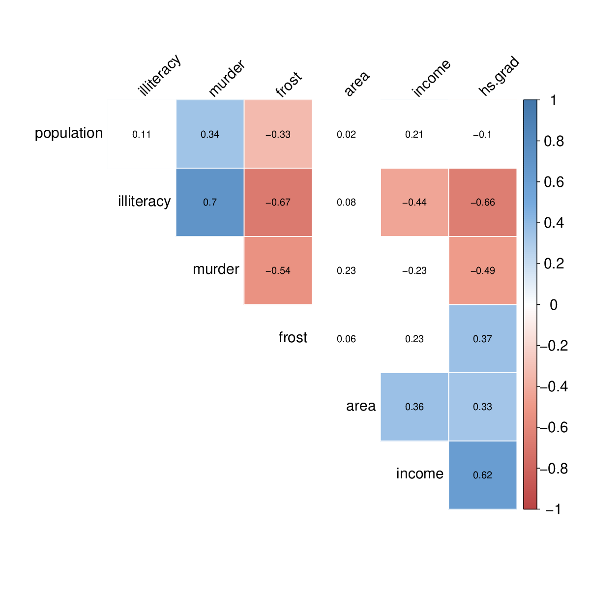
In Figure 3, we plot the coefficients of correlation among covariates. We also show the degree of correlation with colours, and the cells which has not any colour indicate that it is not significant with . According to this figure, there are strong relationship among some predictors. This situation encouraged us to use our suggested estimator since they perform superiorly.
Figure 3. Correlations among predictors
In any application, if we do not have any prior information about covariates whether they are significantly important or not, one might do stepwise or variable selection techniques to select the best subsets. In this study, we use AIC method, we find that income, illiteracy and area variables do not significantly explain the response variable, and these covariates may be ignored. Hence, we fit the sub-model with the help of this auxiliary information, and the full and candidate sub-models are given in Table 4.
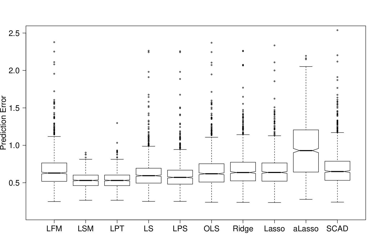
Figure 4. Prediction errors of listed estimators based on bootstrap simulation
Our results are based on bootstrap samples resampled times. Since there is no noticeable variation for larger number of replications, we did not consider further values. The average prediction errors were calculated via 10-fold CV for each bootstrap replicate. The predictors were first standardized to have zero mean and unit standard deviation before fitting the model. To evaluate the performance of the suggested estimators, we calculate the predictive error (PE) of an estimator. In Figure 4, we plot the prediction errors versus the listed estimators.
Furthermore, we define the relative predictive error (RPE) of in terms of the full model Liu regression estimator to ease comparison as follows
where can be any of the listed estimators. If the RPE is smaller than one, it indicates the superiority to LFM. Table 5 reveals the RPE of the listed estimators. According to Table 5, the sub-model estimator has the smallest RPE since it is computed based on the assumption that the selected sub-model is the true model. As expected, due to the presence of multicollinearity, the performance of both Liu-type shrinkage and pretest estimators are better than the estimators based on criteria. Thus, the data analysis corroborates with our simulation and theoretical findings.
(intercept)
Population
Murder
HS.Grad
Frost
RPE
LFM
70.894
0.202
-1.077
0.335
-0.282
1.000
0.016
-0.029
0.034
-0.061
0.016
0.117
0.153
0.181
0.223
0.175
LSM
70.881
0.234
-1.088
0.385
-0.283
0.788
0.003
0.010
0.020
0.008
0.026
0.104
0.117
0.134
0.134
0.161
LPT
70.882
0.232
-1.088
0.383
-0.283
0.794
0.004
0.008
0.020
0.007
0.026
0.105
0.118
0.136
0.136
0.162
LS
70.889
0.216
-1.091
0.350
-0.286
0.917
0.011
-0.014
0.021
-0.043
0.013
0.110
0.133
0.158
0.176
0.171
LPS
70.889
0.215
-1.086
0.353
-0.283
0.883
0.011
-0.015
0.025
-0.040
0.016
0.110
0.132
0.153
0.169
0.162
LSE
70.879
0.231
-1.112
0.395
-0.298
1.005
0.016
-0.029
0.034
-0.061
0.016
0.117
0.153
0.181
0.223
0.175
Ridge
70.893
0.119
-0.816
0.312
-0.188
0.998
0.015
-0.033
0.058
-0.043
0.048
0.115
0.124
0.190
0.145
0.136
Lasso
70.891
0.128
-0.942
0.281
-0.182
0.984
0.012
-0.055
0.090
-0.063
0.051
0.113
0.119
0.190
0.177
0.156
aLasso
70.888
0.096
-0.464
0.571
-0.079
1.385
0.010
0.104
-0.464
-0.223
-0.079
0.129
0.167
0.364
0.233
0.133
SCAD
70.888
0.141
-1.057
0.259
-0.201
1.026
0.009
-0.083
0.051
-0.117
0.107
0.116
0.140
0.175
0.219
0.187
Table 5.
Estimate (first row), Bias (second row) and standard error (third row) for significant coefficients for the state data. The RPE column gives the relative efficiency based on bootstrap simulation with respect to the LFM.
6. Conclusions
In this paper, we combined the pre-test estimator and Stein-type estimator with the Liu regression method in order to obtain a better estimators in the linear regression model when the parameter vector is partitioned into two parts, namely, the main effects and the nuisance effects such that . Thus, our main interest is to estimate when is close to zero. Therefore, we conduct a Monte Carlo simulation study to evaluate the relative efficiency of the suggested estimators and also we present a real data application. According to both the results of the simulation and real application, we conclude that our estimators have better performance than LSE, ridge and the estimators based on criteria.
Acknowledgement
This research is supported by Necmettin Erbakan University, Scientific Research Projects Unit, Project No: 171215001.
References
Ahmed, (2014)
Ahmed, S. E. (2014). Penalty, Shrinkage and Pretest Strategies: Variable Selection and Estimation. Springer, New York.
Akdeniz and Erol, (2003)Akdeniz, F., and Erol, H. (2003). Mean squared error matrix comparisons of some biased estimators in linear regression. Comm. Statist. Theo. Meth., 32(12), 2389-2413.
Belsley, (1991)
Belsley, D.A. (1991). Conditioning diagnostics. John Wiley and Sons, Inc.
Fan and Li, (2001)Fan, J. and Li, R. (2001). Variable selection via nonconcave penalized likelihood and its oracle properties. Journal of the American Statistical Association. 96,1348 – 1360.
Frank and Friedman, (1993)Frank, I. E. and Friedman, J. H. (1993). A statistical view of some chemometrics regression tools. Technometrics. 35,109 – 148.
Hoerl and Kennard, (1970)Hoerl, A. E., Kennard, R. W. (1970). Ridge Regression: Biased estimation for non-orthogonal problems. Technometrics12. 69 – 82.
Hubert and Wijekoon, (2006)Hubert, M. H., and Wijekoon, P. (2006). Improvement of the Liu estimator in linear regression model. Statistical Papers, 47(3), 471-479.
Johnson and Wichern, (2014)Johnson, R. A. and Wichern, D. W. (2014). Applied Multivariate Statistical Analysis, 6rd Ed. Prentice-Hall.
Judge and Bock, (1978)Judge, G. G. and Bock, M. E. (1978). The Statistical Implications of Pre-test and Stein-rule Estimators in Econometrics. North Holland, Amsterdam.
Kibria, (2012)Kibria, B. G. (2012). Some Liu and ridge-type estimators and their properties under the ill-conditioned Gaussian linear regression model. Journal of Statistical Computation and Simulation, 82(1), 1-17.
Knight and Fu, (2000)Knight, K. and Fu, W. (2000). Asymptotics for
Lasso-Type Estimators. The Annals of Statistics. 28(5),1356 – 1378.
Liu, (1993)Liu, K. (1993). A new class of biased estimate in linear regression. Comm. Statist. Theo. Meth., 22(2), 393-402.
Liu, (2003)Liu, K. (2003). Using Liu-type estimator to combat collinearity. Comm. Statist. Theo. Meth., 32(5), 1009-1020.
R Development Core Team (2010)R Development Core Team (2010). R: A Language and Environment for Statistical Computing. R Foundation for Statistical Computing, Vienna, Austria. ISBN 3-900051-07-0.
Saleh and Kibria, (1993)Saleh, A.K.Md. and Kibria, B. M. G. (1993). Performance of some new preliminary test ridge regression estimators and their properties. Comm. Statist. Theo. Meth., 22(10), 2747-2764.
Tibshirani, (1996)Tibshirani, R. (1996). Regression shrinkage and selection via the lasso. Journal of the Royal Statistical Society. Series B (Methodological), 267-288.
Van De Vijver et al., (2002)Van De Vijver, M. J., He, Y. D., van’t Veer, L. J., Dai, H., Hart, A. A., Voskuil, D. W., … and Bernards, R. (2002). A gene-expression signature as a predictor of survival in breast cancer. New England Journal of Medicine, 347(25), 1999–2009.
Yüzbaşı and Ahmed, (2016)
Yüzbaşı, B., & Ejaz Ahmed, S. (2016). Shrinkage and penalized estimation in semi-parametric models with multicollinear data. Journal of Statistical Computation and Simulation, 1-19.
Yüzbaşı et al., (2017)
Yüzbaşı, B., Ahmed, S.E. and Gungor, M., Improved Penalty Strategies in Linear Regression Models, REVSTAT–Statistical Journal, 15(2)(2017), 251–276.
Zou, (2006)Zou, H. (2006). The adaptive Lasso and its oracle properties. Journal of the American Statistical Association, 101(456), 1418 – 1429.