An alternate composite representation
of the velocity profile
in the zpg turbulent boundary layer
Abstract
A composite representation of the turbulent boundary-layer velocity profile is proposed, which combines a recently determined accurate interpolation of the universal law of the wall with a simple analytical expression of the smooth transition of velocity to a constant value in the outer stream. Several examples are given of application of this representation to DNS and experimental data from the literature, and a conjecture is offered for the asymptotic approach of the velocity to its constant inviscid value.
1 Introduction
Coles’ (1956) uniform representation of the mean velocity profile as the sum of a law of the wall and a law of the wake, after appearing on Vol. 1 of the Journal of Fluid Mechanics quickly became a standard in the analysis of the turbulent boundary layer, both for purposes of its theoretical description and for the interpolation of experimental data and characterization of their properties. Coles’ velocity profile can be written as
| (1) |
where both the wall-normal coordinate and streamwise velocity are expressed in wall units (i.e., they are nondimensionalized using the fluid’s viscosity and friction velocity , and so will be understood hereafter even if the traditional + is omitted), and the wake function , with denoting the outer coordinate and itself expressed in wall units, is normalized so that , ; for it Coles proposed . may be construed to be the complete law of the wall or just its logarithmic portion depending on the range over which (1) is to be applied.
Coles’ law provides a family of composite velocity profiles with two free parameters (or three if the dimensional friction velocity is counted in addition to the dimensionless external velocity and thickness ), which can be fitted to a set of measured velocity data in order to extract its boundary-layer thickness and/or shear velocity, and has ever since been widely adopted for this purpose. Yet (1) was soon recognized to miss the smooth asymptotic approach of the boundary layer to its external constant velocity (so called “corner defect”), and Coles himself later recommended (Coles 1968) that the shear velocity and boundary-layer thickness should be determined from a restricted fitting of the velocity profile excluding both a range of near the wall and a range near . The difficulty is intrinsic in the logarithmic behaviour of the overlap velocity, which diverges as the wall-normal coordinate tends either to zero or to infinity, and does not match the finite value of the external velocity unless the boundary layer is truncated at a finite thickness (or the wake function is allowed to diverge in the opposite direction).
More recently Monkewitz et al. (2007) performed an extensive survey of a large number of data sources for the zero-pressure-gradient (zpg) turbulent boundary layer, confirmed the practical adherence of all these profiles (with exceptions ascribed either to presumable imprecision or to inadequate initial conditions) to a two-parameter family of curves, and proposed an alternate composite representation of the multiplicative rather than additive kind which avoids the artificial truncation at a finite thickness; they achieved this result by combining Padé interpolations of suitable order with Euler’s exponential integral.
2 A compact, uniformly valid composite representation
Purpose of the present note is to illustrate yet another multiplicative composite representation, which in addition to providing similar advantages with a simpler expression, offers an unexpected hint at the asymptotic behaviour of the wake region as it wanes into irrotational flow. Let us take it for granted that the velocity profile (where the Reynolds number may for definiteness be the momentum-thickness Reynolds number ) assumes for at constant the universal form of a law of the wall, . In a boundary layer, for at constant it trivially asymptotes to the constant external velocity (which in the case of (1) was ). The simplest composite expression we can imagine is then a weighted sum of these two asymptotes:
| (2) |
where , with , is some yet unknown (hopefully monotonic and well behaved) weight function that goes from for to for over a characteristic thickness scale (conceptually similar but numerically unrelated to the one in (1)).
For any single given velocity profile, (2) can be made exact by simply inverting it to get the appropriate ; thus we can start by looking at what looks like in typical cases. For the law of the wall we shall adopt the analytical interpolation derived by Luchini (2017b), repeated here in a notation that can be cut-and-pasted in most computer programs or scripts:
| (3) |
or, for , just . We recall from Luchini (2017b) that the deviation of (3) from its own logarithmic asymptote is non-monotonic, crosses 0 at and attains a maximum of at ; thus it may actually be sufficient to assume as suggested in many classical textbooks, or even , for the validity of the logarithmic law provided one is willing to accept an error of this order of magnitude, and does not attempt to evaluate the slope of in the region . For a comparison of (3) with the interpolation provided by Monkewitz et al. (2007) and other historical expressions, the reader is referred to Figure 31 of Luchini (2017b).

On the other hand, a comparison of (3) with a typical boundary-layer profile is provided here in Figure 1, which displays the deviation of the mean velocity from the log law (namely the difference ) for the boundary-layer DNS of Sillero et al. (2013) as compared to (3). This figure ought to rule out any doubts that (3), derived by Luchini (2017b) from an interpolation of parallel-flow data after the pressure-gradient correction of Luchini (2017a), applies just as well to the zpg boundary layer.

Armed with from (3), we can now go back to the composite expression (2). Figure 2 reports several curves for the weight function as extracted from the numerical simulation results of Simens et al. (2009); Jimenez et al. (2010); Borrell et al. (2013); Sillero et al. (2013) and Schlatter & Örlü (2010), each normalized on a thickness such that . Though not identical, these curves are indeed close enough to each other that they can reasonably be interpolated by a single monotonic, satisfactorily smooth function.

In fact the shape of this function looks familiar, and might at first sight be mistaken for a gaussian, but Figure 3 points out that a gaussian, the exponential of , is not a good fit. However a little trial and error shows, in the same figure, that the exponential of does fit within an error comparable to the dispersion of Figure 2, in a manner that looks more convincing than an accidental coincidence. This is the interpolation we presently propose:
| (4) |
which compares well to Coles’ wake function as to simplicity, but without any corner singularity in . While (4) is very unlikely to hold literally, its good fit does bear two immediate consequences: one is that the combination of (2), (3) and (4) provides a very compact practical interpolation of a turbulent boundary-layer velocity profile without corners; the other is a suggestive cue that, although an asymptotic trend deduced from empirical data can never be taken for certain, , and not some other exponential, may be the actual asymptotic law with which the mean velocity profile of the boundary layer approaches its inviscid value. Let us consider each of these consequences in turn.

an expression with two free parameters, and , which can be used just like Coles’ and to fit an empirical profile and determine its boundary-layer thickness (and, trivially, external velocity). For instance, a least-square fitting of (5) to the data of Jimenez et al. (2010) produces a velocity profile graphically undistinguishable from the original (Figure 4). We note that the fit has been straightforwardly performed on the whole dataset with no exclusions.

Alternately, if is also regarded as an unknown parameter, (5) can be seen as an expression with three degrees of freedom and used to estimate the wall shear from the velocity profile, in a sophisticated version of Clauser extrapolation. Doing so for the experimental profile SW981127K of Österlund (1999) at nominal produces the example in Figure 5, with a small but possibly significant correction to with respect to the original value (Figure 6). Which one of the two estimates of is to be preferred may be open to discussion, or perhaps even be irrelevant, but again we stress that these figures are produced as a fit of the whole dataset with no exclusions.

3 Outer behaviour and Clauser similarity
Just like Coles’ original formula, the composite formula (5) can be separated, if so desired, into its inner and outer behaviour. For , in the inner wall layer, both formulas trivially reduce to as they are designed to, and hardly any additional remark is needed.
For (say, ), in the outer defect layer, may be replaced by , where we use and in agreement with (3) and Luchini (2017a), and thus (5) becomes
| (6) |
Clauser’s similarity (or equilibrium) regime, generally expected to occur as the Reynolds number (and with it the thickness expressed in wall units) becomes bigger and bigger, requires to be a function of only. This requirement is achieved here if in this limit , constant being in fact the same that would be identified as in (1). Whether Clauser similarity is achieved in any given set of numerical or experimental data can easily be ascertained in the present context by plotting as a function of , after extracting both parameters from a fit of (5) to the data. An example such plot is given in Figure 7.
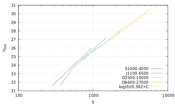
As may be seen, whereas Clauser similarity is conceivably well obeyed in the experiments, the - line has a significantly different slope in both sets of numerical simulations. Whether this is an effect of Reynolds number (but notice that the slope is different even where the Reynolds ranges overlap) or a forewarning of some other discrepancy is open to further investigation.
4 Conclusion: a conjecture on asymptotic behaviour
The success of (5) as a uniform interpolating formula leads to the conjecture that may in fact be the appropriate asymptotic behaviour of the velocity defect at the outer edge of the zpg boundary layer.

In further support of this law of asymptotic decay, Figure 8 depicts the profile of Reynolds stress (whose outer value in wall units tends to as ) compared to the exponential . That this graph too fits reasonably well the same exponential might partially be expected, on the basis of the ties of Reynolds stress with the velocity gradient (viscous stress) in the parallel momentum equation, but it is not totally obvious if it is remembered that in the boundary layer there is an additional convective, thickness-growth, term and that in the laminar regime this term provides the contribution that balances lateral diffusion; in the turbulent boundary layer, longitudinal thickness growth is even stronger. Therefore Figures 3 and 8, together, lend some credibility to the admittedly bold but fascinating conjecture that the exponential , and not or some other exponent, provides the appropriate asymptotic decay of turbulent-boundary-layer mean quantities into the irrotational outer stream.
There is hardly a theory (or perhaps too many theories) to compare this conjecture to, but we can recall that in the laminar boundary layer (and more generally in all diffusion-dominated phenomena), approach to the constant outer state is always like a gaussian (possibly multiplied by a small algebraic power depending on the precise quantity we are looking at); therefore the change in exponent denotes a stark departure from diffusive behaviour. Whether faster-than-diffusive mixing, a known generic property of turbulence, should a priori produce a faster-than-laminar or slower-than-laminar decay of the velocity defect is again not obvious; the present empirical observation of a faster decay is somewhat surprising to be found in a region characterized by entrainment and intermittency in its time evolution, but it should be remembered that the spatial decay of the average is not necessarily the same as the spatial decay of instantaneous quantities. Having a candidate exponent for such decay, nonetheless, might open the roadway to new and exciting interpretations in the future.
References
- Borrell et al. (2013) G. Borrell, J.A. Sillero, J. Jimenez (2013) A code for direct numerical simulation of turbulent boundary layers at high Reynolds numbers in BG/P supercomputers. Comp. & Fluids 80, 37–43.
- Coles (1956) D. Coles (1956) The law of the wake in the turbulent boundary layer. J. Fluid Mech. 1, 191-226.
- Coles (1968) D. Coles (1968) THe Young Person’s guide to the data. A survey lecture prepared for the 1968 AFOSR-IFP-Stanford Conference on Computation of Turbulent Boundary Layers.
- Jimenez et al. (2010) J. Jimenez, S. Hoyas, M. P. Simens, Y. Mizuno (2010) Turbulent boundary layers and channels at moderate Reynolds numbers. J. Fluid Mech. 657, 335–360.
- Luchini (2017a) P. Luchini (2017a) Universality of the turbulent velocity profile. Phys. Rev. Lett. 118, 224501.
- Luchini (2017b) P. Luchini (2017b) Structure and interpolation of the turbulent velocity profile in parallel flow. Preprint https://arxiv.org/abs/1706.02760 submitted to Eur. J. Mech. B/Fluids.
- Monkewitz et al. (2007) P.A. Monkewitz, K.A. Chauhan, H.M. Nagib (2007) Self-consistent high-Reynolds- number asymptotics for zero-pressure-gradient turbulent boundary layers. Phys. Fluids 19, 1–12.
- Österlund (1999) J. M. Österlund (1999) Experimental Studies of Zero Pressure-Gradient Turbulent Boundary-Layer Flow, Ph.D. thesis, Department of Mechanics, Royal Institute of Technology, Stockholm.
- Schlatter & Örlü (2010) P. Schlatter, R. Örlü (2010) Assessment of direct numerical simulation data of turbulent boundary layers J. Fluid Mech. 659, 116–126.
- Sillero et al. (2013) J.A. Sillero, J. Jimenez, R.D. Moser (2013) One-point statistics for turbulent wall-bounded flows at Reynolds numbers up to . Phys. Fluids 25, 105102.
- Simens et al. (2009) M. P. Simens J. Jimenez, S. Hoyas, Y. Mizuno (2009) A high-resolution code for turbulent boundary layers. J. Comp. Phys. 228, 4218–4231.