Glassy states: the free Ising model on a tree
Abstract
We consider the ferromagnetic Ising model on the Cayley tree and we investigate the decomposition of the free state into extremal states below the spin glass temperature. We show that this decomposition has uncountably many components. The tail observable showing that the free state is not extremal is related to the Edwards-Anderson parameter, measuring the variance of the (random) magnetization obtained from drawing boundary conditions from the free state.
I Introduction
It is well known that the Ising model on a regular Cayley tree undergoes a second order phase transition at the critical temperature , below which the Gibbs states and , corresponding to and boundary conditions, are different extremal states. Unlike the usual -lattice case, on the tree the behavior of the free state , corresponding to empty boundary conditions, is very rich. On we have , while on the tree that is trivially true only in the uniqueness regime. Moreover, the free state is extremal for temperatures below the critical temperature , until a certain spin-glass temperature , below which it stops to be extremal. The question of finding the temperature range of the ergodicity of the state was open for twenty years, and was solved by Bleher, Ruiz and Zagrebnov in their 1995 paper [2]. Soon after, a simpler argument was provided by Ioffe, [11]. For a closely related communication theory problem, see the ”Broadcasting on trees” paper by Evans, Kenyon, Peres and Schulman [7].
In the present paper we study the free state at temperatures below .
A principal static feature of the spin glass phase is the presence of infinitely many pure states; see the discussion in [14] and the references therein. By a gauge transformation the spin glass on the tree and the ferromagnet are equivalent, except that random boundary conditions for the ferromagnet correspond to fixed boundary conditions for the spin-glass, as was for example discussed in [3]. We show that the same phenomenon also happens in the ferromagnetic Ising model on the tree, i.e., without randomness in the interaction. Namely, the free state of the Ising model below the spin-glass temperature has a decomposition into extremal states which involves uncountably many extremal states. That is why we call this state ‘glassy’. Our result answers an older question of Arnout van Enter, [15].
The next section contains the more detailed question with some notations and definitions. Our main decomposition result is given in Section 3. The remaining sections contain further details and proofs.
II Notations and definitions
Let be the Cayley tree with branching ratio We consider the nearest neighbor Ising model, where spins have a Gibbs distribution at temperature with boundary condition in a finite volume given by
| (1) |
Both sums run over nearest neighbors pairs, the first being over the pairs
,
, and the second one runs over sites . The infinite-volume Gibbs distributions are obtained as the convex hull of the set of all possible limit point when grows to cover all the vertices of the tree.
The set of Gibbs distributions for a fixed temperature and interaction is convex, and its extreme points are called pure states: they cannot be decomposed into other states.
In the ferromagnetic case we put , while in the spin-glass model the interaction is random: with probability independently for any pair . We can also consider the random interaction
| (2) |
which interpolates between the ferromagnetic model and the spin-glass
model .
It is well known that in the ferromagnetic case the phase transition happens at the critical temperature . For there is a unique infinite-volume Gibbs distribution and below that critical temperature the spontaneous magnetization becomes nonzero, while plus and minus boundary conditions give rise to different states:
We use the convention that the boundary condition by which the infinite-volume Gibbs state is obtained is indicated by a subscript to the expectation , and superscripts will be used to indicate further parameters like temperature or the choice of model in (2).
There is yet another special temperature, , called the spin-glass temperature. It will often appear in what follows below, and it has various interpretations. For the ferromagnetic model it is known that the free state, the infinite-volume Gibbs distribution obtained by putting in (1), is extreme for while it is not for ;
see [2],[11],[7],[13].
Hence the question that motivates the present paper: what is the decomposition
of the free state (at these lower temperatures) into extremal ones?
Part of the question is also to understand why that extremality of the free state exactly stops at the spin-glass temperature, which in its origin characterizes a transition to glassy behavior in the spin-glass model. For example consider the spin-glass state obtained via plus-boundary conditions and look at the (random) local magnetization at the origin:
It depends on the independent random variables , which take values with equal probability. The spin-glass temperature is that temperature below which is a fluctuating quantity with a non-trivial distribution. For example, the second moment, the Edwards–Anderson parameter, is positive only there:
where the expectation is taken over the randomness .
III Decomposition of the free state
In this section we present the decomposition of the free state into pure states and we explain that a continuum of them enters into it, at least at low temperatures. Presumably, it is the case for all temperatures in the spin-glass region.
III.1 The construction of the decomposition
For any Gibbs state corresponding to temperature we have that
where is a spin configuration drawn from and used as boundary condition at infinity. The Gibbs distributions are
-almost surely extreme. Hence, we have here a decomposition of into extreme Gibbs distributions, but obviously the states
might well be the same for
different -s. Nevertheless this decomposition is nontrivial when is not extremal. It remains then to see how many and which different extremal states we get.
For the Ising model free state we will use the Edwards-Sokal representation, [10]:
| (3) |
(In contrast to the more standard notation we prefer here to call the
probability of removed (or closed) bonds.) On the tree, the random
cluster measure is generated by independent bond percolation and is
the resulting random bond configuration over which we take the expectation . The open bonds generate a partition
of the tree into maximal connected components. The measure is supported by the spin configurations which
are constant on each connected component as specified by these
constants take values , independently with probability 1/2.
We can rewrite (3) on the tree by ordering the components using the following definitions.
Let be
a subset of bonds of the tree , and consider the two Ising
spin configurations on defined as:
| (4) |
and
That is, we fix the value of the spin at the root (say ) to be or , and the nearest neighbor spins alternate iff the corresponding bond belongs to the set .
By we denote the Gibbs state of the ferromagnetic Ising model at inverse temperature with the boundary condition where corresponds to the way the spin at the origin is chosen.
Let . Take the set to be random: every bond decides to be in with probability independently of the other bonds. Denote by the expectation with respect to that process.
Proposition III.1.
The following decomposition of the free state for the ferromagnetic Ising model on the tree holds for all temperatures :
| (5) |
where
Proof.
We apply the Edwards-Sokal representation (3) of the Ising model. Start by noting that
Consider now for a given bond collection the atomic measure , which to assigns two configurations defined by the relations (4), each with probability In other words, fixing the spin of the origin and fixing determines all the other spin values, where in particular neighboring connected components of open bonds alternate their spin. However the resulting spin configuration would have the same distribution as in the Edwards-Sokal representation with twice as large probability of closed bonds: with ,
Bringing all that together we conclude that on the tree (3) reduces to the formula (5). ∎
Note also that the states , can be obtained as thermodynamic limits of the finite-volume Gibbs states with the boundary conditions , . These limits exist for -almost all boundary conditions , .
To see that this decomposition (5) is non-trivial for it suffices to show that when , for -typical sets . That follows from the relations
| (6) |
which are a special case of the Theorem 1.1 of [7].
Of course, the states may coincide for different sets – this is the case at high temperature. In the next subsection we will show that at low temperatures there is a continuum of different states as we vary over the sets , see also [8]. There we have shown that if the set consists of bonds sufficiently separated from one another, then the configuration is a stable ground state. Of course, for our random configuration this is not the case; for example we will see in pairs of bonds sharing a vertex, which will happen with positive density. However, quite often we will see just isolated bonds, well separated, once is small enough, see the next subsection for more details.
Remark. At all temperatures the free-state two-point function goes to zero when goes to infinity, yet for the free state is not extreme. In particular, the magnetization in increasingly large volumes has a variance that does not go to zero with the size of the volume. The interesting tail-observable which shows that the free state is not extreme is related to the Edwards-Anderson parameter. Here is the simplest version: take the magnetization at the origin,
in the infinite-volume Gibbs distribution with boundary condition ; that is drawn from the free state at temperature . For the random variable has a non-trivial distribution.
III.2 At low temperatures the states are mutually singular.
Theorem III.2.
Pick two independent configurations , from the distribution . Then the two limiting states , exist and are mutually singular a.s. with respect to , provided the temperature is low enough.
Proof. We denote by a random configuration of bonds in each bond picked independently with probability with the parameter being fixed and small enough. We will study the Gibbs states at low temperatures, with the goal of showing their a.s. mutual singularity.
Let be a bond, and be a ball of radius centered at Consider the ground state (=zero temperature Gibbs) measure in the box with boundary condition We call the bond frustrated in the state if the event happens with probability one in the state for all large enough. We call the bond to be -strongly-frustrated (or just -frustrated) in the state if the event happens with probability one in the state as well as the events for all bonds within distance from the bond again for all large enough.
For example, the above will hold if while is a deterministic configuration composed from isolated bonds which are sufficiently far away from each other, see [8], [9]. What we want to show now is that if is random, and then it is very likely that is -frustrated, provided is small enough (depending on ). Once we show that, our claim about mutual singularity will be proven, since for two independent configurations we will be able to find arbitrarily large disjoint sets of -frustrated bonds.
So let be random, and Our first observation is that the probability of having other bonds at distance from is quite small, provided is small enough. That would be the end of the story if the configuration would be a ground state configuration. Indeed, in that case the state would be a small perturbation of the configuration once is low, uniformly in
However, the configuration is not a ground state configuration a.s., so the state might have other frustrated bonds in moreover, it even can happen that itself is not frustrated in this state. We will show now that all this is highly unlikely, once is small enough.
So suppose the set of frustrated bonds of the state is not the singleton That can happen iff there is a contour crossing certain number of bonds of such that Consider the set of the bonds of which are inside and the set of bonds of the contour is intersecting. Together they form a finite tree which has the same branching number as our infinite tree The set is the set of all leaves of the tree Let be the number of nodes of inside and be the intersection So we have and
Evidently, the probability of seeing such a tree
so
The number of trees with inner nodes does not exceed Thus the probability that a given bond is a leaf of such a tree with leaves is bounded from above by
which is exponentially small in for small enough. So we can apply the standard Peierls argument to shows that the probability of the event
goes to zero as which ends the proof.
To conclude, we point out for clarity that the “Gibbs ground” states constructed from the -random bond configurations , are typically nontrivial measures, i.e. they have infinite supports, a.s. This is in contrast with the ground states constructed in [8], where the corresponding Gibbs ground states are supported by a single ground state configuration. However, as is explained above, a vast majority of the frustrated bonds under typical ground state are isolated bonds, once is small. This fact is the source for the decomposition (5) to have a continuum of extremal components.
IV Double–temperature Ising model
We already mentioned in the introduction that the phase diagram of the ferromagnetic Ising model is essentially determined by the critical temperature , and the spin-glass temperature . A clarification of the situation can however be obtained by enlarging the objects in (5) into a two-temperature setting. We consider two-temperature states, with the bulk temperature and the boundary temperature,
which is the infinite-volume Gibbs distribution at temperature with the boundary condition taken to be the spin configuration (4) where is drawn from , the Bernoulli bond percolation process with parameter .
Of course, one may wonder whether the thermodynamic limits exist.
We are not going to prove it; what is said below holds for any limit point of that family. Note that (5) contains these states with – and that is why it is useful to speak about the temperature , but of course the relevant parameter is the density . The following is therefore presented in the -plane, which is also the setting of [4].
Consider the curve
Note that when .
Proposition IV.1.
For any positive temperature and parameter ,
- 1.
When , the expected local magnetization of the random Gibbs states vanishes,
- 2.
When ,
Let us now look at the second moment, , which is called the Edwards-Anderson (EA) parameter.
Proposition IV.2.
For the random Gibbs state
- 1.
If and , then
- 2.
Otherwise, for any other temperature :
Moreover,
which means that the EA random variable is non-degenerate.
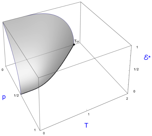
From Fig. 2 it is clear that the model shows an interesting and non-trivial behavior even on the line
That case is treated in [1].
To understand the nature of the spin-glass temperature, we remark that the composition , which we abbreviate as
is an involution: . In particular,
Let us prove the last two Propositions in the vicinity of the point After the analysis of the section III.B and using its technique, it is almost immediate.
Let us fix to be the root of our tree. Informally speaking, the magnetization at the root in the state is defined by the few bonds of the (rare) bond configuration which are in some proximity to Moreover, this magnetization will take different values when these few bonds happen to be different. Since that happens with positive probability, our claim follows.
To be more formal, let be the ball of radius centered at Let be a bond in Define the set as the family of all realisations which has as the only bond in Clearly, the probability is positive for every value of the parameter Now, let be two such bonds, with and let be two typical configurations. Then, using the technique of the section III.B and a little of cluster expansions, one sees that there exists a constant such that
provided both and are small enough. That proves the positivity of the variance of the EA random variable (with randomness coming from ).
The proofs in general case involve the recursion relations, and can be obtained from the results of the papers [5], [6]. These results are summarized graphically by the following pictures.

Acknowledgments Part of this work has been carried out in the framework of the Labex Archimede (ANR-11-LABX-0033) and of the A*MIDEX project (ANR-11-IDEX-0001-02), funded by the “Investissements d’Avenir” French Government programme managed by the French National Research Agency (ANR). Part of this work, concerning the EA parameter, has been carried out at IITP RAS. The support of Russian Foundation for Sciences (project No. 14-50-00150) is gratefully acknowledged. This work was partially supported by the CNRS PICS grant “Interfaces aléatoires discrètes et dynamiques de Glauber” and by the grant PRC No. 1556 CNRS-RFBR 2017-2019 ‘Multi-dimensional semi-classical problems of Condensed Matter Physics and Quantum Mechanics ”. CM thanks the hospitality of the CPT-Luminy at Marseille.
References
- [1] P.M. Bleher, The Bethe Lattice spin glass at zero temperature. Ann. Inst. Henri Poicaré. 54: 89-113 (1991).
- [2] P.M. Bleher, J. Ruiz, and V. Zagrebnov, On the purity of the limiting Gibbs state for the Ising model on the Bethe lattice. J. Stat. Phys. 79, 473–482 (1995).
- [3] J.T. Chayes, L. Chayes, J. P. Sethna, and D. J. Thouless, A mean field spin glass with short rang interaction. Commun. Math. Phys. 106: 41-89 (1986).
- [4] J.M. Carlson, J.T. Chayes, L. Chayes, J. P. Sethna, and D. J. Thouless, Critical behavior of the Bethe lattice spin glass. Euophys. lett. 5: 355-360 (1988).
- [5] J.M. Carlson, J.T. Chayes, L. Chayes, J. P. Sethna, and D. J. Thouless, Bethe lattice spin glass: the effects of a ferromagnetic bias and external fields. I. Bifurcation analysis. Journal of statistical physics 61, no. 5-6 (1990): 987-1067.
- [6] J.M. Carlson, J.T. Chayes, L. Chayes, J. P. Sethna, and D. J. Thouless, Bethe lattice spin glass: the effects of a ferromagnetic bias and external fields. II. Magnetized spin-glass phase and the de Almeida-Thouless line. Journal of statistical physics 61, no. 5-6 (1990): 1069-1084.
- [7] W. Evans, C. Kenyon, Y. Peres, and L.J. Schulman, Broadcasting on trees and the Ising model. Annals Appl. Prob. 10 N° 2: 410-433 (2000).
- [8] D. Gandolfo, J. Ruiz, and S.B. Shlosman, A Manifold of Pure Gibbs States of the Ising Model on a Cayley tree. J. Stat. Phys. 148: 999-1005 (2012).
- [9] D. Gandolfo, J. Ruiz, and S.B. Shlosman, A Manifold of Pure Gibbs States of the Ising Model on the Lobachevsky plane. Commun. Math. Phys. 334, 313-330 (2015)
- [10] H.-O. Georgii, O. Häggström, and C. Maes, The random geometry of equilibrium phases, Phase Transitions and Critical Phenomena, vol 18, Eds C. Domb and J.L. Lebowitz (Academic Press, London) pp 1-142, 2001.
- [11] D. Ioffe, A note on the extremality of the disordered state for the Ising model on the Bethe lattice. Lett. Math. Phys. 37: 137-143 (1996).
- [12] R. Bruce King, Beyond the Quartic Equation. Birkhaüser Boston, (1966).
- [13] F. Martinelli, A. Sinclair, and D. Weitz, Glauber dynamics on trees: boundary conditions and mixing times. Commun. Math. Phys. 250: 301-334 (2004).
- [14] C.M. Newman and D.L. Stein, Short-range spin glasses: results and speculations. Lecture notes in Mathematics, Springer-Verlag 1900, (2007).
- [15] Aernout Van Enter, Private communication, (2007).