The HIP 79977 debris disk in polarized light
Abstract
Context. Debris disks are observed around 10 to 20 % of FGK main-sequence stars as infrared excess emission. They are important signposts for the presence of colliding planetesimals and therefore provide important information about the evolution of planetary systems. Direct imaging of such disks reveals their geometric structure and constrains their dust-particle properties.
Aims. We present observations of the known edge-on debris disk around HIP 79977 (HD 146897) taken with the ZIMPOL differential polarimeter of the SPHERE instrument. We measure the observed polarization signal and investigate the diagnostic potential of such data with model simulations.
Methods. SPHERE-ZIMPOL polarimetric data of the 15 Myr-old F star HIP 79977 (Upper Sco, 123 pc) were taken in the Very Broad Band (VBB) filter ( nm, nm) with a spatial resolution of about 25 mas. Imaging polarimetry efficiently suppresses the residual speckle noise from the AO system and provides a differential signal with relatively small systematic measuring uncertainties. We measure the polarization flux along and perpendicular to the disk spine of the highly inclined disk for projected separations between (25 AU) and (200 AU). We perform model calculations for the polarized flux of an optically thin debris disk which are used to determine or constrain the disk parameters of HIP 79977.
Results. We measure a polarized flux contrast ratio for the disk of in the VBB filter. The surface brightness of the polarized flux reaches a maximum of at a separation of along the disk spine with a maximum surface brightness contrast of . The polarized flux has a minimum near the star because no or only little polarization is produced by forward or backward scattering in the disk section lying in front of or behind the star. The width of the disk perpendicular to the spine shows a systematic increase in FWHM from (12 AU) to , when going from a separation of to . This can be explained by a radial blow-out of small grains. The data are modelled as a circular dust belt with a well defined disk inclination and a radius between and 90 AU. The radial density dependence is described by with a steep (positive) power law index inside and a more shallow (negative) index outside . The scattering asymmetry factor lies between and 0.6 (forward scattering) adopting a scattering-angle dependence for the fractional polarization such as that for Rayleigh scattering.
Conclusions. Polarimetric imaging with SPHERE-ZIMPOL of the edge-on debris disk around HIP 79977 provides accurate profiles for the polarized flux. Our data are qualitatively very similar to the case of AU Mic and they confirm that edge-on debris disks have a polarization minimum at a position near the star and a maximum near the projected separation of the main debris belt. The comparison of the polarized flux contrast ratio with the fractional infrared excess provides strong constraints on the scattering albedo of the dust.
Key Words.
Planetary systems – Scattering – Stars: individual object: HIP 79977, HD 146897 – Techniques: high angular resolution, polarimetric1 Introduction
Many main-sequence stars with circumstellar dust have been identitified based on the detection of infrared (IR) excess emission (Aumann et al., 1984; Oudmaijer et al., 1992). For nearby systems with strong IR excess, like Pic, Fomalhaut, HR 4796A and others, it was shown with high contrast observations that this dust is located in disks or rings (Smith & Terrile, 1984; Backman & Paresce, 1993; Schneider et al., 1999; Kalas et al., 2005) around the central star. The dust is attributed to dust debris from collisions of solid bodies in a planetesimal disk, similar to the Kuiper belt in the solar system (see e.g., Wyatt, 2008, for a review). The lifetime of small dust particles, which are the main component for the IR-excess emission, is very short because they are blown out of the system by radiation pressure or stellar winds and therefore they must be replenished by ongoing collisions in the system. Bright debris disks are particularly frequent around young stars where they are the last phase of the evolution of planet-forming disks and for this reason young, bright giant planets are often found in systems with debris disks (Kalas et al., 2008; Marois et al., 2008; Lagrange et al., 2010, e.g.,). For older stars ( yr) the debris disks are rare and usually faint with a few interesting exceptions which could be caused by a strong transient collisional event. Debris-disk structure has the potential to reveal the dynamics of planetary systems and provide very important information about their evolution.
Important aspects for an understanding of the parent bodies responsible for the debris dust are the disk geometry and the dust particle sizes, structures, and compositions. The determination of the geometry requires spatially resolved observations of the disk. This can be achieved with IR-observations of the thermal emission of the dust (Stapelfeldt et al., 2004; Su et al., 2005; Wahhaj et al., 2007, e.g.,), or with high-contrast observations of the scattered stellar light (Golimowski et al., 2006; Schneider et al., 2014, e.g.,). Particle properties are difficult to derive observationally, because the measurements are indirect and often ambiguous. Typical particle sizes may be inferred from the spectral energy distribution in the IR and the separation of the dust from the star. For hot dust, the composition can sometimes be inferred from spectral features, mainly the silicate bands around 10 m and 18 m (Chen et al., 2006; Duchêne et al., 2014; Mittal et al., 2015; Olofsson et al., 2009; Moór et al., 2009; Olofsson et al., 2012, e.g.,) and the color of the scattered light might also indicate grain size, porosity or composition of the particle (Debes et al., 2008; Debes et al., 2013, e.g.,).
Up to now, most high-resolution and high-contrast images of debris disks in scattered light have been taken with the Hubble Space Telescope (HST) or adaptive optics (AO) observation using large telescopes from the ground. HST is a powerful high-contrast instrument because the point spread function (PSF) is not affected by a turbulent atmosphere and therefore it provides well calibrated intensity images of extended disks. AO observations from the ground provide a high spatial resolution but they suffer from the variable PSF which depends strongly on atmospheric conditions. To reveal faint debris disks, high-contrast data-reduction techniques like angular differential imaging (ADI) or reference PSF subtraction must be applied. This can be particularly difficult for ground-based AO data.
In this work we present data of the debris disk HIP 79977 which was observed with differential polarimetric imaging using the new, extreme AO instrument SPHERE-ZIMPOL at the VLT (Beuzit et al., 2008). Polarimetry is an alternative and very sensitive differential measuring method for accurate measurements of the polarized and therefore scattered light from circumstellar dust in the bright halo of unpolarized light from the central star. The measured polarization signal contains additional diagnostic information on the scattering dust, different from the intensity signal. But the diagnostic potential of polarimetry has hardly been investigated for debris disks because only a few systems have been observed with polarimetry up until a few years ago (Gledhill et al., 1991; Tamura et al., 2006; Graham et al., 2007; Hinkley et al., 2009). With the advent of new extreme AO systems, such as SPHERE and Gemini Planet Imager (GPI), with sensitive polarimetric modes (Perrin et al., 2015; Olofsson et al., 2016; Draper et al., 2016, e.g.,) this technique will become much more attractive. Our data on HIP 79977 are also used to demonstrate the capabilities of SPHERE-ZIMPOL for debris disks with imaging and polarimetric imaging. Therefore, we provide more extensive information on data reduction, analysis, and modeling.
HIP 79977 is a young, 15 Myr old (Pecaut et al., 2012),
F2/3V star of the Upper Scorpius association, located at
a distance of 123 pc (van Leeuwen, 2007). The 1.5
star is not known to have stellar or planetary companions so far. The infrared excess was detected by the IRAS satellite and was associated with a bright debris disk based on the 24 m and 70 m excesses measured with Spitzer Multiband Imaging Photometer (MIPS) (Chen et al., 2011). The authors supported their suggestion with the high-resolution optical spectra obtained with Magellan MIKE spectrograph which showed no signs of active accretion onto the star. There is not much gas in the disk because only
a tentative detection of the CO gas was reported by Lieman-Sifry et al. (2016),
suggesting that the amount of gas in the disk is
small compared to the amount of dust. The fractional IR luminosity of
of this target is
high but not exceptional. Among 46 young F-type stars of the Scorpius-Centaurus OB Association with mass 1.5 and age between 10 and 17 Myr which were identified as debris disk systems, 11 show a fractional IR luminosity higher than (Jang-Condell et al., 2015).
The disk around HIP 79977 was imaged in scattered light intensity, or Stokes , in the H-band
and also detected with polarimetry
with the Subaru HiCiao instrument (Thalmann et al., 2013). The
observations revealed an edge-on disk extending out
to approximately 2′′ (250 AU), though its inner regions () were hidden by
residual speckles.
These data show that HIP 79977 is a good case for an
edge-on debris disk fitting well onto the detector
field of view () of the SPHERE-ZIMPOL instrument.
Similar full disk observations are not possible with this instrument for the famous
nearby examples Pic or AU Mic, because they are
too extended.
The paper is organized as follows. In Sect. 2 we describe the observations and present the data. Section 3 is dedicated to the methods of the data reduction and Sect. 4 to the polarimetric data analysis. Then, in Sect. 5, we give a description of our model for the spatial distribution of the dust developed to reproduce the morphology of the HIP 79977 debris disk and present the results of the modeling. Finally, in Sect. 6, we compare results from this work with the disk models obtained in previous studies of HIP 79977 and discuss the diagnostic potential of polarimetric measurements of debris disks.
| Date/Observation | Instrument | Filter | Filter | Integration Time [s] | Observing Conditions | |||||
|---|---|---|---|---|---|---|---|---|---|---|
| identification | mode | arm 1 | arm 2 | DIT1 | Tot2 | Eff3 | Airmass | Seeing [′′] | [ms] | |
| 2014-08-15/ | ||||||||||
| OBS227_0003-0006 | imaging | VBB | I_PRIM | 60 | 2400 | 1740 | 1.00–1.01 | 0.9–1.7 | 1.7–2.8 | |
| 2015-04-24/ | ||||||||||
| OBS114_0122-0200 | SP | VBB | VBB | 16 | 5120 | 3872 | 1.03–1.27 | 1.1–2.2 | 0.9–1.8 | |
1 Detector integration time (DIT).
2 Total integration time on source.
3 Total integration time of all frames used in the data reduction.
2 Observations
The SPHERE “Planet Finder” instrument for high-contrast observations in the near-IR and visual spectral range consists of an extreme adaptive optics (AO) system and three focal plane instruments for differential imaging (Beuzit et al., 2008; Kasper et al., 2012; Dohlen et al., 2006; Fusco et al., 2014). The data described in this work were taken with the ZIMPOL (Zurich Imaging Polarimeter) subsystem working in the spectral range from 520 nm to 900 nm (Schmid et al., 2012; Bazzon et al., 2012; Roelfsema et al., 2010). The SPHERE-ZIMPOL configuration provides a spatial resolution of mas and observing modes for angular differential imaging and polarimetric differential imaging. The pixel scale of ZIMPOL is 3.60 mas per pixel and the field of view is . ZIMPOL has two camera arms, cam1 and cam2, and data are taken simultaneously in both arms, each equipped with its own filter wheel.
A special feature of the ZIMPOL detectors is the row masks covering every second row of the detector which is implemented for high-precision imaging polarimetry using a polarimetric modulation and on-chip demodulation technique (Schmid et al., 2012). A raw frame taken in imaging mode has only every second row illuminated and the useful data has a format of pixels where one pixel represents mas on the sky. The same format results from polarimetric imaging for the perpendicular and parallel polarization signals stored in the “even” and “odd” rows respectively. The advantage of this technique is that the images with opposite polarization and are recorded using the same detector pixels. This significantly reduces the differential aberation between and and flat-fielding issues. In the data reduction the and frames, each pixels, are extracted. In a later step in the reduction the pixel images are expanded into pixel images with a flux conserving interpolation so that one pixel in the reduced image corresponds to mas on sky.
All SPHERE-ZIMPOL observations of HIP 79997 are summarized in Table 1.
Imaging observations of HIP 79977 were carried out during a SPHERE commissioning run in August 2014 using the VBB or RI-band filter ( nm, nm) in cam1 and the I-band filter ( nm, nm) in cam2. A sequence of 40 frames with a total exposure time of 40 min was taken in pupil tracking mode for angular differential imaging (Marois et al., 2006, ADI;). The atmospheric conditions were strongly variable with a seeing between 0.9′′ and 1.7′′ and short coherence times between 1.7 and 2.8 ms.
Polarimetric measurements were taken as part of the SPHERE guaranteed time observations (GTO) on April 24, 2015 in field stabilized instrument mode (P2) and using the slow polarimetry (SP) detector mode with modulation frequency 27 Hz. The wide VBB filters were used in both arms of the instrument. We observed the target with four different sky orientations on the CCD detectors with position-angle offsets of and with respect to sky North. We recorded several polarimetric QU-cycles for each position angle. In one cycle, the half-wave plate (HWP) is rotated by 0∘, 45∘, 22.5∘ and 67.5∘ for measurements of the Stokes linear polarization parameters , and , respectively. In total 320 frames with an on-source integration time of about 85 min were taken. The observing conditions for the polarimetric observations were strongly variable with rather poor seeing conditions (varying from 1.07′′ to 2.23′′) and passing clouds, so that the AO system loop crashed repeatedly. Figure 1 shows the registered source counts illustrating the variable atmospheric extinction.
The peak of the stellar PSF is saturated by at most a factor of 10 in the center ( pixels) for the imaging and also the cloud-free polarimetric observations. Non-coronagraphic, moderately saturated observations were chosen to optimize the dynamical range of the data at small angular separation with not too much sensitivity loss at large separation due to read-out noise.
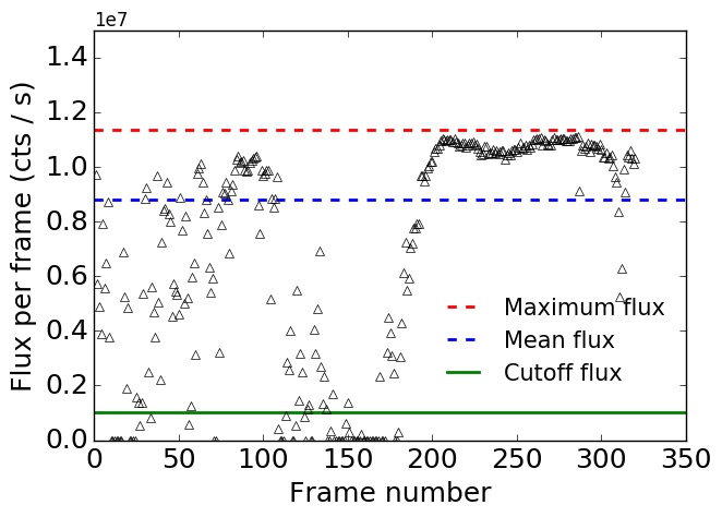
3 Data reduction
3.1 Angular differential imaging
For the basic data reduction steps of images of total intensity (Stokes ) taken in 2014, the SPHERE Data Reduction and Handling (DRH) software (Pavlov et al., 2008) was used. This includes the image preprocessing, dark frame subtraction and flat-fielding. All 40 frames were visually inspected and 11 bad frames containing strongly asymmetric PSFs and unexpected features were rejected (see Table 1 for the total effective integration time after frame selection). These effects were caused by phases when the control loop of the AO system failed or almost failed because of the “rough” atmospheric conditions. To reduce the impact of strong PSF variations, all selected frames were rescaled by dividing them by the flux measured in an annulus between pixels and pixels.
We used a LOCI algorithm (Locally Optimized Combination of Images, Lafrenière et al. (2007)) to remove the stellar light from the images. LOCI divides each frame into segmented annuli; for each segment, it then constructs a matching reference PSF from a linear combination of similar segments taken from other frames in the dataset. The two most important tuning parameters of the algorithm are and . The former determines the degree to which point sources in the data are protected from self-subtraction: frames are excluded from the linear combination if their differential field rotation with respect to the working frame is so small that a planet located in the working annulus would move by less than times the Full Width at Half Maximum (FWHM) between the two frames. The second parameter, , describes the size of the region in which the optimization is performed in units of resolution elements.
When optimized for point-source detection, LOCI causes dramatic self-subtraction and therefore signal loss in extended structures such as circumstellar disks. However, the parameters can be adapted to preserve more disk flux while still maintaining some of the algorithm’s efficacy at speckle removal (“conservative LOCI”). Here, we adopt a small value of and a large value of , which has proven effective in past studies (Thalmann et al., 2010; Buenzli et al., 2010; Thalmann et al., 2011, e.g.,).
Scattered light from the debris disk is detected in the I-band and VBB data along a line oriented in ESE – WNW direction which is slightly offset from the star towards SSW. Emission is visible from to beyond from the star as shown in Fig. 2. The LOCI reduction can be interpreted as an edge-on disk with a high inclination . At small separations from the star the southwest side of the disk is bright while the northeast side is not detected. The main disk features observed by us confirm the H-band observation of Thalmann et al. (2013) but our data provide a higher spatial resolution and S/N-detection.

3.2 Polarimetric differential imaging
The data have been reduced with the SPHERE-ZIMPOL software developed at the ETH Zurich. The basic reduction steps are essentially identical to the SPHERE DRH software.
The polarimetric data were also visually inspected and correctly recorded frames with count rates above were selected for the data reduction. The total integration time after removing bad frames is 3872 s (see Table 1).
The ZIMPOL is designed as sensitive imaging polarimeter and it includes a series of differential techniques to reduce systematic effects for the detection of faint polarimetric signals (Bazzon et al., 2012; Thalmann et al., 2008). This includes the combination of polarimetric modulation and a synchronous on-chip demodulation where opposite polarization modes and are stored with charge shifting in the “odd” and “even” detector pixel rows on the CCD. Furthermore, every second frame reverses the up and down shifting to account for charge shifting differences, and every -frame is complemented with a -frame to compensate the instrumental polarization. These steps are intrinsic parts of the observing strategy.
A basic data reduction is often sufficient to identify a bright circumstellar disk. Sometimes, better results can be obtained if also the residual telescope polarization is taken into account. This is a more difficult task, because and the orientation of this polarization depends on color, rotation mode P1 or P2, and pointing direction and the correction law is not available yet. A preliminary analysis of the calibration with zero-polarization standard stars indicates a telescope instrumental polarization at the level of . A useful work-around provides a forced normalization of the total counts of corresponding frames, for example, or . However, such procedures can introduce spurious signals and must be applied with caution because they treat the intrinsic polarization of the central star or an interstellar polarization signal like a (instrumental) telescope polarization signal.
Early ZIMPOL-SPHERE observations demonstrate that the basic reduction steps combined with the forced normalization trick yield high-quality polarimetric images of proto-planetary disks (Garufi et al., 2016; Stolker et al., 2016). However, one should be aware, that the contrast of even a bright debris disk like HIP 79977 is about one order of magnitude lower than a bright proto-planetary disk. For this reason additional systematic effects need to be corrected.
Systematic noise from the instrument can also be reduced by averaging data taken with different field orientations. We have taken such data for HIP 79977 but the improvement is limited because certain position angles were strongly affected by clouds. Important for the quality of the final result is a careful centering of individual images to a high precision. This works well with a fit of a two-dimensional (2D) Gaussian function to the steep intensity gradients of the stellar profile, despite the often saturated central peak. The estimated centering accuracy is pixels or mas.
Finally, we found that the combination of the final frames from cam1 and cam2 is also very beneficial for the image quality. Spurious polarization signals introduced by temporal variations of the atmosphere and AO system are opposite in the two channels if the same filters are used in cam1 and cam2 so that in a mean image some temporal effects are compensated.
After all these data reduction steps, significant signals of polarized light from the debris disk are clearly visible in the Stokes and images (Fig. 3). The central star is marked with an asterisk, and the white circle shows the immediate region surrounding the star which is affected by saturation and strong speckle noise.
The and images both show a faint negative halo around the central star. This could be explained by a residual polarization signal of % and % of the stellar PSF in the and images respectively which could be the result of the applied “forced normalization” described above. This effect can be corrected by:
| (1) |
| (2) |
where and are mean stellar intensities measured in and cycles respectively.
Diffraction from the telescope spider could be an additional effect contributing to the observed halo. The orientation of the vertical telescope spider coincides during the polarimetric observations with the negative regimes above and below the disk in Q and U images. Further characterization of the instrument is needed to understand the origin of this signal.
Azimuthal polarization images:
From the Stokes Q and U maps we can compute the intensity of the polarized flux . However, is affected for low signal-to-noise data by a systematic bias effect because of squaring of and parameters. Therefore we characterize the disk polarization pattern with a locally defined azimuthal / radial - and -parameter definition with respect to the central light source as discussed in Schmid et al. (2006). Single scattering off dust particles in optically thin debris disks generates linearly polarized light with the electric field vector azimuthally oriented with respect to the star. Polarization in the azimuthal direction is defined by the Stokes parameter :
| (3) |
where is the polar angle between north and the point of interest measured from the north over east. The Stokes parameter :
| (4) |
defines the polarization pattern in the directions with respect to the direction.
Figure 4 shows the final and . The
image clearly reveals the nearly edge-on disk structure down
to a projected separation of .
Polarized light is detected across the entire width of the
image of . The peak of the surface brightness
appears here as a narrow stripe below the expected major axis of an inclined circular ring
(white dotted line) with a flux minimum near the position of the star.
By contrast, the image contains no structural features from the disk. Assuming azimuthal polarization of light generated in single scattering processes and no multiple scattering (Canovas et al., 2015, see), we do not expect to find any astrophysical signal in the image. Therefore, this image can be used for an estimation of the statistical pixel to pixel noise level and large-scale systematic errors in our observations.
Very close to the star, marked by a white circle with a (Figs. 3 and 4), the data are unreliable because of strongly variable wings of the PSF peak. Also visible are the faint features at above and below the disk which are negative in the and images, and appear as positive signal in the and images. These features are much fainter (factor < 0.1) than the disk signal and originate most likely from poorly corrected instrumental effects because an intrinsic signal is expected to produce no signal.

4 Data analysis


4.1 Disk position angle
We measured the position angle of the disk in the -image by the determination of the orientation of the mirror line through the central star perpendicular to the disk. The best position angle was found by searching with an angle increment of 0.1∘ the orientation of the mirror line which produces the smallest residuals if one side is subtracted from the other side.
The results from the polarimetric and imaging data sets agree. After including ZIMPOL’s True North offset of we obtain the position angle of the disk axis to be . This value is in good agreement with PA = reported by Thalmann et al. (2013) for the scattered light images in H-band and with PA = measured by Lieman-Sifry et al. (2016) in the sub-mm range.
We define an disk coordinate system where the star is at the origin, is the coordinate along the major axis in roughly WNW-direction (), towards ESE (), and perpendicular to this with the positive axis towards NNE (or EoN). The disk images in Figs. 2 and 4 and the plot coordinates in Figs. 5 and 6 are given in this system.
Scattered light images of edge-on disks after classical ADI, LOCI or PCA-ADI reductions suffer from the disk flux over-subtraction particularly in the regions close to the star. The degree of flux loss depends on the shape of stellar PSF and, hence, on the observational conditions. This also applies to the total intensity image of the disk shown in Fig. 2. In contrast, the intensity of the polarized light in the image is not strongly affected by the data reduction and better suited for the analysis of the disk structure. Therefore, in the following sections, we study, model and discuss the distribution of the polarized surface brightness based on the image.
4.2 Polarized light brightness profiles vertical to the disk


Vertical separation from the disk major axis

Figure 5 shows the vertical brightness profiles at different separations from the star which are obtained from the image by applying a wide binning of 30 pixels (108 mas) in -direction and a narrow binning of 3 pixels in -direction. Obviously, the disk structure is very similar or symmetric on the east-southeast (ESE) and west-northwest (WNW) sides of the disk, with strongly peaked vertical profiles at small separations 0.5" ( 60 AU) and weak and broad profiles at large separations ( 87 AU). The innermost profiles at and also slightly at are affected by the residual instrumental features restricted to small -coordinates.
The vertical profiles can be fitted well by the Moffat function (Trujillo et al., 2001)
where is the flux peak located at a vertical distance from the disk major axis. The parameter and exponent are related to the FWHM by
We used a non-linear least squares algorithm to find the best fit parameters for the vertical Moffat profiles.
Figure 6 shows the -dependence of the vertical profiles along
the major axis of the disk. The top panel (Fig. 6(a))
demonstrates the nearly identical decrease of the profile’s peak
as a function of the projected separation for both sides of the
disk. The profiles with the highest peak flux lie between . The results of our measurement of interior
cannot be considered as reliable because of the residual speckle noise and detector
saturation effects.
As shown in Fig. 6(b), the disk
width is continuously increasing with separation from
about (10 AU) at (25 AU)
to (37 AU) at (100 AU). At
" the disk width is not well defined but the ESE side seems to
be broader than the WNW side. The points beyond are not
included in this estimate because of the low SNR at large separation.
The blue line in Fig. 6(c) gives the vertically integrated polarized flux per -interval (width 108 mas) along the major axis. The integration in -direction is from to for each x-bin. The blue dots are the same but the integrated flux is derived from the fitted Moffat profiles. According to this, the maximum brightness in polarized light of the edge-on disk in HIP 79977 is at a separation of (74 AU). There is a very small discrepancy between data and fit for because the Moffat profile cannot fit correctly negative flux values at small angular separations which originate from the systematic effects described above.
The vertical offset of the disk spine is shown in Figure 6(d). The spine curve is roughly symmetric with respect to . The smallest -offset is approximately mas (2.5 AU) around . Closer to the star, , the spine is further away from the major axis with mas, and also in the outskirts () the -offset is even more than 50 mas. In comparison, the offset of the disk spine measured in the imaging data (Fig. 2) is approximately mas (7.5 AU) at . For larger separations, the -offset in intensity is smaller and achieves a minimum mas at .
4.3 Polarized flux, surface brightness and contrast
The polarimetric image in Fig. 4 and the deduced profiles in Fig. 6 serve as basis for the quantitative determination of the polarized flux and surface brightness of the disk which can both be compared to the stellar brightness with “contrast” parameters.
We derive the total polarized flux of the debris disk by summing up all the bins from to 1.8′′ along the major axis in the integrated flux profile given in Fig. 6(c). This does not include the innermost regions . Only a small polarization signal is expected at small apparent separations for a disk or ring with an inner radius , because at small separations we observe scattering from the disk sections located in front of and behind the star. This forward and backward scattering produces only little polarization. Thus, one can approximate the innermost disk with a linear extrapolation of the measured curve from to (red dotted line in Fig. 6(c)).
This neglects a possible contribution of polarized flux from warm dust located very close () to the star. Studies on the spectral energy distribution of HIP 79977 (Chen et al., 2011, e.g.,) indicate that there is no significant () signal to the IR excess emission from warm dust at small separation. Therefore, we assume that there is also no significant unresolved contribution from an inner disk to the polarization signal.
The polarized flux in the VBB filter, covering an effective aperture area of and including the interpolated points inside interval , amounts to 5800 counts per second and per ZIMPOL arm. This value must be corrected for the variable atmospheric transmission (Fig. 1) using a factor of . This yields a corrected count rate of 7540 800 cts/s where the uncertainty is dominated by .
The determination of the stellar flux of HIP 79977 must account for the saturation of the PSF core and the cloudy weather. We first determine the mean value of cts/s in the VBB filter for frames 210-280 which were apparently not affected by clouds (Fig. 1). Because the exposure is saturated out to the radius px some flux is lacking. To account for the saturated part of the PSF, we compare the HIP 79977 profile with high-quality ZIMPOL PSFs of the standard star HD 183143 (Schmid et al., 2017, STD261_0013-24, ), which were taken under excellent atmospheric conditions. For the narrow band filters N_R ( nm, nm) and N_I ( nm, nm), these PSFs contain within a radius of px a flux between % and % of the total stellar flux measured for an aperture of diameter. Based on this, we assume for our HIP 79977 data, that the round annulus with inner and outer radii px and px ( diameter) contains between % and % of the flux expected for an unsaturated PSF profile. This yields for the corrected stellar count rates between cts/s and cts/s per ZIMPOL arm for observations in the VBB filter in the slow polarimetric mode.
The count rates are converted to photometric magnitude (VBB) using the following expression (Schmid et al., 2017):
where am is the airmass, is the filter coefficient for the atmospheric extinction, is the photometric zero point for the VBB filter and is an offset to the zero point which accounts for the used instrument and detector mode. We obtain for HIP 79977 a magnitude = 8.60 in good agreement with the literature values (see Table 2). The derived photometric magnitude yields the color V-VBB = 9.09m - 8.60m = 0.49m which is close to the color index in the Johnson-Cousins’ photometric system (Pecaut et al., 2012, = 0.806 m, m for ; ) for a F2/3V star.
| Filter | mag | Ref. | |||
|---|---|---|---|---|---|
| (m) | (m) | (mag) | (mag) | ||
| HIP HP | 0.528 | 0.221 | 9.20 | <0.01 | 1 |
| Tycho V | 0.532 | 0.095 | 9.11 | 0.02 | 2 |
| Johnson V | 0.554 | 0.082 | 9.09 | <0.01 | 1 |
| Gaia G | 0.673 | 0.440 | 8.93 | <0.01 | 3 |
| ZIMPOL VBB | 0.735 | 0.290 | 8.60 | 0.07 | 4 |
| Johnson J | 1.250 | 0.300 | 8.06 | 0.02 | 5 |
Notes: (1) ESA (1997); (2) Høg et al. (2000); (3) Gaia Collaboration (2016); (4) this work; (5) Cutri et al. (2003).
For the polarized flux of the whole disk we get
= 16.6m 0.3m. This yields a ratio
of total polarized flux of the disk to the stellar flux of .
We determine for the peak surface brightness of the polarized light arcsec-2 along the inner () disk spine (Fig. 6(a)) and a surface brightness contrast for the polarized flux of mag arcsec-2. For the outer disk around the surface brightness contrast is about 10 mag arcsec-2.

5 Modeling
To reproduce the physical appearance of the debris disk around
HIP 79977 we construct a 3D model
for the scattered intensity and the polarization flux from optically thin (single scattering) dust.
The disk is described by an axisymmetric dust distribution
using the cylindrical coordinates and h,
where and
describe the disk midplane and the axis gives the height above it
(see Fig. 7). The disk
model is projected onto an x-y sky plane,
where defines the line of nodes and y is the
perpendicular axis through the central star. The -axis is
equivalent to the line of sight to the star and the z-component is important for
the calculation of the scattering
angle . The disk coordinates are related to the sky coordinates by:
,
Following Artymowicz et al. (1989) we adopt a product of two functions to describe the number density distribution n(r, h) of dust grains in the disk
For the radial R(r) and vertical Z(h) distribution profiles we adopt expressions which are often used in the literature (Augereau et al., 2001; Ahmic et al., 2009; Thalmann et al., 2013) in accordance with the theory of a "birth ring", a planetesimal reservoir in analogy to the Kuiper Belt in the solar system. In this ring, dust down to sub-micron sizes is produced by collisions and evaporation of solid bodies. The radial profile is given by the following expression:
| (5) |
where is the radius of planetesimal belt and radial power laws and describe the increase of grain number density inside the "birth ring" and the decrease of the density in the outer region, respectively. The vertical profile Z(h) defines an exponential drop-off with the disk height:
| (6) |
where for a purely exponential fall off and for the Gaussian profile. For the scale height we assume a power law dependence on radius
where is a scale height at and is the flare index of the disk.
For an optically thin debris disk the amount of scattered radiation from a volume element with coordinates is determined by the intensity of the incident light at wavelength and the product of the average grain cross-section for scattering per particle with the number density of grains in this volume. How much light is scattered by particles into the specific direction depends on the scattering angle :
and is described by the phase function . We derive the intensity of the light in the computed image from the integral over all grid cells along the line of sight or z-axis
| (7) |
where denotes the HIP 79977 monochromatic luminosity at wavelength , is the star-Earth distance and is an averaged
dust scattering phase function (see Sect. 5.1).
The grain cross-section for scattering is a product of the grain geometrical cross-section with the grain-scattering efficiency .
In general, the scattering efficiency as well as the phase function depend
on the wavelength of the incident light and the grain size, shape and composition. Assuming the same composition and shape parameters for all grains in the unit volume with coordinates , we can average over all particle sizes to express per particle as
| (8) |
where is a grain radius varying between the minimum size and maximum size for a given grain size distribution , and defines the differential number density of grains with radii in the interval . The grain minimum and maximum sizes have to be fixed in our model if the phase function is calculated from the Mie scattering theory. In detailed treatments these parameters can vary freely but in order to reduce the running time of the code, we simplify the computation of the scattering cross-section by considering the same grain-size distribution, grain sizes and optical properties everywhere in the disk. In this case the average cross-section per particle is constant through the disk and we can take it out of an integral:
| (9) |
where is a normalization parameter containing all constants used in the model, such as the HIP 79977 luminosity and the star-Earth distance, and so on.
In this work we concentrate on the polarized scattered light from the debris disk. Therefore we need to model the polarized flux, which requires the consideration of a different scattering phase function together with the corresponding angle dependence of the produced polarization signal as discussed in the following subsection. The result follows then from the integration
| (10) |
where is the scaling factor .
The model images for the different polarization components , , and must be convolved with an instrument PSF before being combined to the model images of the Stokes parameters which can be compared with the observations. Because the PSF shape is strongly variable, we selected a mean PSF which is representative for the observations. This mean PSF was fitted with a radial, rotationally symmetric Moffat profile which was used for the convolution. The exact shape of the stellar PSF is not so critical because our disk models have a relatively simple structure.
5.1 The scattering phase function for polarized light
The phase function (PF) in Equation (7) characterizes the angle dependence of scattered radiation. In the following, we disregard the wavelength dependence of the PF.
A very popular way to describe the scattering phase function is the Henyey-Greenstein (HG) function (Henyey & Greenstein, 1941):
| (11) |
where is the average of the cosine of the scattering angle which characterizes the shape of the phase function. For isotropic scattering , forward scattering grains have , while for the scattering is peaked backwards.
However, there exists also growing evidence that a simple HG-function is a poor approximation for the modeling of the scattered intensity from debris disks. This is nicely demonstrated for the bright disk HR 4796A (Milli et al., 2017), which shows, for small phase angles , a strong diffraction peak and, for large phase angles , a scattering intensity which is roughly angle-independent. Thus, a more general phase function, for example, a two-component (or double) HG function seems to be required for the modeling of the scattered intensity of highly inclined debris disks
| (12) |
where the first term describes the strong diffraction peak, the second term represents the more isotropic and much less forward scattering part (Min et al., 2010, see also), and is the scaling parameter, .
For the polarized scattered radiation from a debris disk the situation is slightly different. The strong forward peak seen in intensity, which can be ascribed to the light diffraction by large particles , is expected to produce no significant light polarization. The scattering polarization is produced by the photons hitting the particle surface and interacting by diffuse reflection or/and refraction and transmission as described above by the second term . But, in addition, the angle dependence of the linear polarization produced by the particle scattering needs to be taken into account. For example, strict forward and backward scattering will produce no polarization for randomly oriented particles for symmetry reasons. We adopt the Rayleigh scattering function as a simple approximation for the angle dependence of the polarization fraction :
with the scaling factor , which defines the maximum fractional polarization produced at a scattering angle of .
Figure 8 shows some examples of obtained phase function for the polarized flux for different cases of the HG function . For isotropic scattering () the maximum of scattered polarized flux occurs at . For an asymmetry parameter the maximum is shifted to smaller scattering angles producing a corresponding asymmetry in the amount of polarized light received from the front and back sides of the disk. So, for example, the value of polarized flux PF () at is 35 times higher than at .
5.2 Model fitting
We have calculated models for a parameter grid as specified in Table 3 in order to find the set of model parameters which best fit the observed polarized intensity image.
For the fitting, we reduced the number of image pixels by binning and selected a rectangular image area with a length of 341 and width of 100 binned pixels centered and aligned to the disk x and y (major and minor) axes (see Fig. 9(d)). A round area with a radius of 16 pixels (0.17′′) centered on the star and the spurious features near the saturated region are excluded from the evaluation of the fit goodness. Figure 9 illustrates the different steps in the image fitting procedure. From the model dust distribution in the disk (a) the expected polarization flux is calculated (b), convolved with the instrument PSF (c), fitted to observation (d), and the residuals (e) are then used for the evaluation of the image fit.
The goodness of the fit was estimated for each model with the reduced -parameter:
where is a number of data points with measurement results which have uncertainties .
Each data point corresponds to a binned pixel within the minimization window shown in Fig. 9(d). denotes
the number of free parameters used to create a model image with
values and listed in Col. 1 of Table 3.
To accelerate the fitting procedure we have made a preselection of disk models using the mean disk profile along the major axis shown in Fig. 10. The mean profile consisting of 15 points from to for the observed disk polarization is obtained by averaging the data points from the negative and positive -axes given in Fig. 6(c). Thus the 2D models were collapsed to a profile and fitted first to the profile calculating the and defining a good fit threshold based on the number of degrees of freedom for the fit (Press et al., 2007).
The procedure is straight forward because the noise is well defined for these data points which represent flux integrations over a large area. This can also be inferred from the observed profiles for the two disk sides, which look essentially identical, indicating that there are no localized spurious effects or strong intrinsic asymmetries in the disk. The fitting does not depend on uncertainties in the PSF model convolution because the spatial resolution is low. Still, the key properties of the geometric distribution of the polarized flux along the disk spine are captured by the -profile.
Models with a are considered to fit the -profile well (see the examples in Fig. 10). The profile fitting is compatible with a disk with a radius in the range [60, 86] AU which coincides with the separation of the maximum. Of course, the fitting of disk models described by 9 parameters to a 15 point profile cannot define a unique solution for HIP 79977 disk but provides more or less well defined ranges for the model parameters.
The scaling factor (see Table 3) is determined by the minimization of the -profile fit for each model. This approach has been chosen because the statistical noise is larger and not well known systematic uncertainties are much harder to quantify for the image data points.


In a second step, we compare the 2D disk models which were preselected by the previous profile fitting to the image (Fig. 9(d)) to further constrain the model parameters. This provides a multidimensional parameter distribution of well-fitting models by setting a threshold for the 2D image fit . The mean values of the obtained distribution are adopted as the best-fit model parameters. Their uncertainties are given by the 68% marginalized errors as calculated from the sample covariance matrix. The mean parameters together with the confidence intervals are listed in Table 3 (Col. 5 and Col. 6, respectively). The corresponding synthetic image of polarized light is shown in Fig. 9(b) and the convolved image (Fig. 9(c)) appears to fit the image (Fig. 9(d)) well. The residuals image (Fig. 9(e)) displays some PSF-shaped leftovers, the instrumental features above and below the disk center and, possibly, some minor residues from the disk flux. In this case the model would lack flux along the spine at small separation.
| Parameter | Range | Step of linear | Best model | Model 70 | Model 40 | |
|---|---|---|---|---|---|---|
| sampling | mean value | 68% CL | ||||
| Radius of belt (AU) | [30, 90] | 10 | 73 | 16 | 70 | 40∗ |
| Inner radial index | [1, 10] | 1 | 5.0 | 2.8 | 2.0∗ | 2.0∗ |
| Outer radial index | [-6, -1] | 0.5 | -2.5 | 1.4 | -3.0 | -2.5 |
| Scale height (AU) | [0.5, 3.5] | 0.5 | 2.3 | 0.7 | 1.5 | 0.5∗ |
| Vertical profile | [0.5, 2.5] | 0.5 | 0.9 | 0.6 | 1.0 | 1.0 |
| Flare index | [0.5, 4.5] | 1 | 2.2 | 1.4 | 2.5 | 3.5 |
| Inclination | [82, 87] | 1 | 84.6 | 1.7 | 85.0 | 82.0∗ |
| HG parameter | [0.0, 0.9] | 0.1 | 0.43 | 0.25 | 0.20 | 0.20 |
| Scaling factor | - | - | 9.04 | - | 4.03 | 3.10 |
Notes: ∗ Parameter value lies outside the 68% confidence interval.
Our modeling assumes that the optical depth in the disk is small. According to our best-fit model we estimate a for a radial photon path through the disk midplane (), and significantly less for . After scattering, a photon escapes without further interaction because we see the disk inclined by with respect to edge on.
Our statistical analysis of the model fitting allows an assessment of the parameter degeneracy problem where many different combinations of parameters match the data. In particular we notice an important degeneracy between the radius of the planetesimal belt and scattering asymmetry parameter . Figure 12 shows the 68% and 95% confidence level (CL) regions derived from the distribution of these two parameters. The contours cover an extended region implying that the degeneracy between the radius of the planetesimal belt and asymmetry parameter cannot be resolved with our data.
To examine how well/badly models other than the mean model reproduce the data, we compare two models randomly picked from the generated distribution: one model (specified in Table 3 as "Model 70") with all parameters lying inside of the 1- area with the belt radius AU close to the mean value of this parameter, and one model (specified in Table 3 as "Model 40") with the same but AU lying outside of the 1- range. Figure 11 shows both models in four different views: dust distribution in the disk , non-convolved model image of the polarized flux, polarized image produced after the combination of convolved intensities , , , . with the instrumental PSF.
"Model 40" gives a significantly worse fit for the central part of the image compared to "Model 70" based on the derived and visual examination of the residues. The comparison of the disk polarization profile of “Model 40” with the observations also shows a relatively poor match (see Fig. 10). "Model 70" gives a reasonable fit to the polarization profile and also the residuals in the 2D image appear to be not much larger than the best-fit model, as is expected for a model within the 1 confidence area.


6 Discussion
6.1 Disk structure
Our results from the modeling of the dust distribution around HIP 79977 indicate a mean radius of 73 AU for the planetesimal belt. The vertical distribution of the dust in the disk is described by a profile with an exponent smaller than two. This is a steeper fall-off than a Gaussian distribution, indicating a higher concentration of particles in the midplane. The radial distribution of the grain number density matches the shape of an annular disk with an inner cavity. This assumption is supported by the SED of HIP 79977 showing no significant thermal emission at wavelengths m. The depletion of scattering material inside a possible belt of parent planetesimals can be caused by the radiation pressure or drag forces acting on small particles (Wyatt, 2008, and references therein).
The radiation pressure pushing outward the dust grains with sizes close to or smaller than the blow-out size (< 1 m) could be responsible for the growing width of the disk vertical cross-sections when the separation from the star increases from to (Fig. 6(b)).
In the past years several authors have derived a distance of the dust grains from the star in HIP 79977 by modeling the shape of the disk SED with a single- or double-temperature fit. Assuming that the dust grains emit radiation like black bodies, Chen et al. (2011) have determined a dust grain temperature of 89 K based on the Spitzer MIPS photometry. They considered amorphous silicates with olivine composition as the main component of the dust, and the average size of the grains, which were not removed by the radiation pressure, to be 1.5 m. They have estimated that if the grains are spherical and in radiative equilibrium they should be located at a distance of at least 40 AU from the star. In reality, the bulk of the dust could have a larger radial separation because the real dust grains emit radiation less efficiently than black bodies. Dust with the same equilibrium temperature can therefore exist at larger distances from the star. This supports our mean model indicating a separation which is more like 70 AU.
Jang-Condell et al. (2015) postulated a much larger average grain size of 11.1 m based on an analysis including Spitzer IRS spectra. They derived a grain temperature of 102 K (for amorphous silicates with olivine composition) requiring a stellocentric distance of about 11.5 AU for the grain distribution which is in conflict with our results.
Previous imaging and polarimetric imaging of the disk around HIP 79977 in the H-band was presented by Thalmann et al. (2013). From the data they derived a disk orientation of 114∘ (major axis), and an inclination of 84∘ in very good agreement with this work. Thalmann et al. (2013) modelled the self-subtraction effects for flux extraction for the intensity image and derived the intrinsic intensity slope for the disk along the major axis. In addition, they detected a polarimetric signal from the disk for separations from to , compared the polarization with the intensity profile and found a fractional polarization of (-range [5 %, 20 %]) at and ([30 %, 60 %]) at . From their data, it is not clear whether or not they see in polarized flux a maximum at a separation of around and a flux decrease inside. Thalmann et al. (2013) also fit the observations with model calculations but they adopt a radius of AU for the planetesimal ring and do not investigate models with larger .
The new SPHERE - ZIMPOL observations presented in this work provide a very much improved polarimetric sensitivity which clearly reveals a maximum in the polarization profile at a projected separation of 0.60 (74 AU). This maximum location is not compatible with the small ring radius of AU adopted by Thalmann et al. (2013), probably, because they only fit the intensity profile which shows no features that could constrain the ring radius.
Our best-fit model is in good agreement with results of recent observations of HIP 79977 with ALMA. Lieman-Sifry et al. (2016) used the 1240 m continuum visibilities and derived basic geometrical parameters of the disk. They modelled the surface density of the disk with a single power law extending from an inner to an outer radius and they derived AU without detecting an outer cut-off radius. This result confirms the large ring radius found by us from the polarimetric profile. Lieman-Sifry et al. (2016) also measured a disk inclination and which are consistent with our and previous results.
6.2 Diagnostic potential of polarimetry
The scattered flux has been measured for more than 20 debris disks, mainly with the Hubble Space Telescope (HST) (Schneider et al., 2014; Schneider et al., 2016, e.g.,). With ground-based observations the flux measurement for the scattered light from debris disks is very difficult because of the speckle noise introduced by the atmospheric turbulence. The polarized flux of the disk is much easier to determine, because it is a differential quantity which can be distinguished from the unpolarized light from the bright central star (), even in the presence of strong atmospheric speckles.
For HIP 79977 the disk profile in polarized flux reveals a clear maximum which traces the radial location of the disk ring. This information is difficult to obtain from intensity imaging of edge-on disks, because the Stokes I disk profile is dominated by the forward scattering dust in front of the star and therefore the projected disk extension may not be visible.
The disk flux and the polarized flux contain complementary information about the scattering dust. The scattering angle dependence is strongly different because forward and backward scattering produces no or only very little polarized flux. This applies also to the diffraction peak (or forward scattering peak) from large particles , which is not or only slightly polarized. This means that the polarized flux originates predominantly from scatterings with scattering angles in the range and the polarized flux produced per scattering event can be approximated by an averaged particle parameter for the induced scattering polarization for the scattering angle of (see Sect. 5.1).
New constraints on dust properties may be obtained if quantitative polarimetric data of many debris disks can be collected. The dust grain size distribution and therefore the polarimetric properties are expected to depend on the spectral type of the central star and different system ages may reveal evolutionary processes in the polarimetric properties of the scattering dust. Polarimetric parameters which can be quantified for the dust are scattering cross-section or albedo, and parameters of the polarimetric scattering function and . A better understanding of the dust in debris disks would be very useful for interpretations regarding the nature of their parent bodies which produced the observed dust in a collisional cascade.

6.2.1 Polarized flux and infrared excess
The reflectivity or scattering albedo of the dust in the debris disk of HIP 79977 can be characterized by a comparison of the scattered polarized flux with the IR excess luminosity which is a good measure for the dust absorption.
In Sect. 4.3, we derived the fractional polarized flux or ratio of total polarized disk flux to the stellar flux . This ratio was obtained for the wide VBB filter near the peak of the stellar energy distribution. Therefore, we can consider the ratio as a good order of magnitude estimate for the fractional polarized light luminosity of the disk expressed as . This statement considers also the fact that depends very little, less than a factor of two, upon the disk inclination.
The fractional infrared excess of HIP 79977 is given in Jang-Condell et al. (2015). This yields the double ratio
where the uncertainty only accounts for uncertainty in the -ratio derived in this paper. The double ratio could be a good proxy for the ratio between the polarized luminosity and the IR-excess luminosity of the disk
if the wavelength and inclination dependence of the dust scattering can be neglected. It is emphasized, that neglecting the wavelength dependence of the polarized flux of the disk may not be an acceptable simplification for some cases, for example, for near-IR polarimetry of disks around A-stars, which emit most of their radiation in the UV-visual spectral region.
Therefore, is an observational parameter that depends, like the scattering albedo, on the ratio between dust scattering cross-section and absorption , and parameters of the polarimetric phase function and as
| (13) |
The inclination dependence of is illustrated in Fig. 13, which shows the polarized flux (expressed per steradian) with respect to the scattered light luminosity excluding the diffracted light. The scattered light interacts with the surface of the dust particles, and, therefore, the asymmetry parameter , which we introduced for the polarized light, is also adopted for the intensity of the scattered light as a first approximation (see Sect. 5.1).
For isotropic scattering and maximum polarization (), the ratio of polarized flux to scattering luminosity is for because the scattering angle for a pole-on disk is throughout and the radiation is 100 % polarized. For larger inclinations (for ) the ratio is smaller, because there is more forward and backward scattering which produces less polarization. The ratio between a pole-on and edge-on disk is . We note that pure Rayleigh scattering is different, because it is not isotropic.
For strong forward scattering the amount of polarized light is reduced with respect to the scattered intensity (see Fig. 8) or the disk luminosity in scattered light (without diffraction). For the polarized flux is therefore almost independent of the disk inclination, and for , edge-on disks are even brighter in than pole-on disks because so much more light is scattered in forward directions.
Figure 13 is independent of the radial mass distribution for rotationally symmetric, flat, optically thin disks and a given scattering phase matrix. The inclination can usually be determined easily. More difficult is the determination of the scattering asymmetry parameter , at least for edge-on disks and pole-on disks. For HIP 79977, the 1- uncertainty range for is [0.2,0.7], and this leaves an uncertainty of about a factor 1.5 (see Fig. 13) for the ratio determination. In addition, there is also the factor , which needs to be known to constrain the mean scattering albedo of the dust in debris disks.
Clearly, there is not a straight-forward way to derive a value for from a polarimetric observation of a single disk. However, we can expect progress if the polarized flux is derived for several disks with different inclinations, including cases where the -asymmetry parameter can be well defined.
Also of great value would be polarimetric observation, for which well calibrated HST intensity images are available to complement the -plot of Schneider et al. (2014, their Fig. 8) with an equivalent plot for the polarized disk flux and constrain differences between scattered intensity and polarized intensity of debris disks.
Up to now there exists only few polarized flux measurements for debris disks and therefore it is difficult to compare different disks. More data will become available soon from the new polarimetric high-contrast observing modes of SPHERE and other similar instruments (e.g., GPI, HiCIAO).

6.2.2 Comparison with the edge-on disk AU Mic
The disk around the nearby (9.9 pc) low-mass star AU Mic (M1Ve) is a very good example of a previous high-quality study of the polarization of an edge-on debris disk. HST imaging for this target is presented by Krist et al. (2005) and Schneider et al. (2014) and imaging polarimetry is described in Graham et al. (2007).
Krist et al. (2005) measure from their AU Mic intensity image a disk width which increases with apparent separations qualitatively similar to the behavior measured from our polarized intensity image for HIP 79977 (Fig. 10). Graham et al. (2007) present a profile of the fractional polarization along the disk spine together with an intensity profile for the F606W filter-band ( = 0.590 m, m). We obtained their profiles (J. Graham, personal communication) and constructed for AU Mic a mean disk profile given in Fig. 14. This profile shows a maximum value and essentially no polarized flux close to the star, again very similar to HIP 79977 (Fig. 10).
In AU Mic, the peak of the polarized flux is at 40 AU and this coincides well with the outer edge of the dust belt seen in the ALMA 1.3 mm dust continuum, which probably traces the outer edge of the suspected “birth ring” of colliding planetesimals (MacGregor et al., 2013). This finding for AU Mic supports our interpretation of HIP 79977 data, that the measured maximum polarization at 75 AU represents well the “birth ring” radius.
The HST polarimetry of Graham et al. (2007) is not flux calibrated and therefore we used the F606W imaging of AU Mic of Krist et al. (2005). They provide a calibrated SB profile of the disk spine and the disk widths at different separations from which we derive a calibrated intensity profile . With this, we calibrate the polarimetry of Graham et al. (2007) and derive for the AU Mic disc in the F606W filter a total polarized flux of mJy. This includes the disk regions from to 11′′ on both sides but not the innermost arcsec. The calculated polarized flux relative to the stellar flux is .
With the fractional infrared luminosity (Plavchan et al., 2009) we obtain a -parameter equal to for AU Mic. It is interesting to note that the debris dust in AU Mic produces approximately five times as much scattering polarization when compared to HIP 79977, if we compare the fractional polarized flux in the F606W filter to the fractional infrared excess.
The interpretation of this difference is not clear. One possibility is, that the blue color of the disk around AU Mic is caused by a surplus of very small grains when compared to other debris disks (Krist et al., 2005). Roughly, the maximum blow-out size scales like the ratio between the stellar luminosity and the stellar mass (Burns et al., 1979). For AU Mic this ratio is about an order of magnitude smaller than for HIP 79977. When disregarding possible small differences in grain properties it implies that the minimum grain size in the disk around AU Mic is about m, in rough agreement with results obtained by Schüppler et al. (2015). The corresponding value is m for HIP 79977. For this reason, the polarized flux derived for the HST F606W might not represent a good wavelength average for the scattering polarization in AU Mic and the derived -parameter must therefore be interpreted with caution.
6.2.3 Dust scattering properties and disk model
In this work the observed polarized flux from the debris disk in HIP 79977 is fitted with disk models. For this, the parameters describing the dust scattering were restricted to for the scattering phase angle dependence for polarized light and for the amount of polarized light produced by the scattering. Unfortunately, it was not possible to constrain these parameters well with the modeling.
The maximum fractional polarization produced per scattering can only be constrained if the intensity of the scattered light from the disk can also be accurately measured. The intensity signal of HIP 79977 is clearly detected with SPHERE-ZIMPOL but this signal is strongly affected by self-subtraction effects of the ADI procedure which are hard to quantify. Therefore, a determination of and needs a more accurate stellar PSF subtraction technique, as is possible with HST.
The asymmetry parameter for the polarized scattered flux is also not well constrained because of the edge-on configuration of the HIP 79977 disk. We clearly see the expected polarization minimum for forward and backward scattering at small angular separation from the star. However, the more subtle asymmetry parameter is not well defined. From the modeling of the polarization profile along the disk spine , it is not possible to disentangle the parameters for the radial distribution of the dust from the scattering asymmetry parameter . Our data show at least that , that is, much more polarized flux is produced in the forward scattering direction because the disk spine in polarized flux is on the same side of the central star, like the intensity spine caused by forward diffraction.
A more accurate determination of will be possible for debris disks with a slightly smaller inclination, where the azimuthal dependence of the polarized flux can be defined.
7 Summary
In this paper, we present SPHERE-ZIMPOL images of polarized light of the debris disk around HIP 79977 in the 590-880 nm wavelength range using differential polarimetry and an intensity image extracted with angular differential imaging using the LOCI-algorithm. We have characterized and analyzed the disk structure, mainly based on the polarized flux image and obtained the following results:
- •
The images show a nearly edge-on disk extending from less than out to the edge of the detector at 225 AU): they unveil regions close to the star which were hidden by residual atmospheric speckles in previous data (Thalmann et al., 2013, cf.).
- •
For the PA of the disk, we measure , which is in a good agreement with the value reported by Thalmann et al. (2013) and Lieman-Sifry et al. (2016).
- •
From our polarimetric data, we derive disk cross-sections perpendicular to the disk midplane. The peaks of the perpendicular profiles are slightly offset ( mas) because we are seeing a strong flux asymmetry between the front and back sides of a highly inclined disk. At small apparent separations () the profiles have a super-exponential drop-off pointing to a well defined concentration of large dust particles in the midplane of the inner disk. The disk width (FWHM) is increasing systematically from (12 AU) to , when going from a separation of to . The growth of the profile scale height could be caused by a radial blow-out of small grains.
- •
The disk surface brightness profile in polarized light along the disk spine is symmetric on the ESE and WNW sides. There is a clear maximum of between and where the surface brightness contrast with respect to the central star is . There is a clear minimum of SB closer to the star (), because no or only little polarization is produced by forward scattering in the disk section lying in front of the star which dominates the signal in the intensity image. The geometric structure of the disk seen in polarized light is consistent with intensity images taken with SPHERE-ZIMPOL and literature data. Unfortunately, it is difficult and we were not able to derive a high-quality intensity profile for the disk and therefore we could not make a quantitative comparison between intensity and polarized flux.
- •
The disk profile in polarized flux for HIP 79977 shows a clear maximum at the projected separation of AU. This seems to be a good measure of the belt radius for this edge-on debris disk.
- •
The disk total polarized flux amounts to = 16.6 0.3 which is .
- •
The ratio compares the disk polarized flux with the disk infrared excess. We emphasize the value of this parameter for the characterization of the scattering albedo of the dust particles. For comparative purposes, we derive the ratio for the edge-on debris disk around the M star AU Mic based on the previous HST observations of this target.
The dust distribution of the disk around HIP 79977 was modelled with a 3D rotationally symmetric belt of radius , with radial power laws for the density fall-off inside and outside and an exponential function in vertical density distribution. A large grid of models was fitted to the data and we derive the best disk parameters using a optimization technique. This model analysis yields a disk with an inclination of and a belt radius AU and a grain density distribution with a steep power law index inside and a more shallow index outside . The derived scattering asymmetry parameter lies between and 0.6 (forward scattering) using an adopted angle-dependence for the fractional polarization like for Rayleigh scattering.
Acknowledgements.
We thank James Graham for providing the AU Mic disk profiles derived from HST data and published in Graham et al. (2007, Fig. 4) in electronic form. We would also like to thank the referee for many thoughtful comments which helped to improve this paper. This work is supported by the Swiss National Science Foundation through grant number 200020 - 162630. SPHERE is an instrument designed and built by a consortium consisting of IPAG (Grenoble, France), MPIA (Heidelberg, Germany), LAM (Marseille, France), LESIA (Paris, France), Laboratoire Lagrange (Nice, France), INAF – Osservatorio di Padova (Italy), Observatoire de Gen‘eve (Switzerland), ETH Zurich (Switzerland), NOVA (Netherlands), ONERA (France) and ASTRON (Netherlands), in collaboration with ESO. SPHERE was funded by ESO, with additional contributions from CNRS (France), MPIA (Germany), INAF (Italy), FINES (Switzerland) and NOVA (Netherlands). SPHERE also received funding from the European Commission Sixth and Seventh Framework Programmes as part of the Optical Infrared Coordination Network for Astronomy (OPTICON) under grant number RII3-Ct-2004-001566 for FP6 (2004–2008), grant number 226604 for FP7 (2009–2012) and grant number 312430 for FP7 (2013–2016). J.O acknowledges support from ALMA/Conicyt Project 31130027, and from the Millennium Nucleus RC130007 (Chilean Ministry of Economy).References
- Ahmic et al. (2009) Ahmic, M., Croll, B., & Artymowicz, P. 2009, ApJ, 705, 529
- Artymowicz et al. (1989) Artymowicz, P., Burrows, C., & Paresce, F. 1989, ApJ, 337, 494
- Augereau et al. (2001) Augereau, J. C., Nelson, R. P., Lagrange, A. M., Papaloizou, J. C. B., & Mouillet, D. 2001, A&A, 370, 447
- Aumann et al. (1984) Aumann, H. H., Beichman, C. A., Gillett, F. C., et al. 1984, ApJ, 278, L23
- Backman & Paresce (1993) Backman, D. E. & Paresce, F. 1993, in Protostars and Planets III, ed. E. H. Levy & J. I. Lunine, 1253–1304
- Bazzon et al. (2012) Bazzon, A., Gisler, D., Roelfsema, R., et al. 2012, in Proc. SPIE, Vol. 8446, Ground-based and Airborne Instrumentation for Astronomy IV, 844693
- Beuzit et al. (2008) Beuzit, J.-L., Feldt, M., Dohlen, K., et al. 2008, in Proc. SPIE, Vol. 7014, Ground-based and Airborne Instrumentation for Astronomy II, 701418
- Buenzli et al. (2010) Buenzli, E., Thalmann, C., Vigan, A., et al. 2010, A&A, 524, L1
- Burns et al. (1979) Burns, J. A., Lamy, P. L., & Soter, S. 1979, Icarus, 40, 1
- Canovas et al. (2015) Canovas, H., Ménard, F., de Boer, J., et al. 2015, A&A, 582, L7
- Chen et al. (2011) Chen, C. H., Mamajek, E. E., Bitner, M. A., et al. 2011, ApJ, 738, 122
- Chen et al. (2006) Chen, C. H., Sargent, B. A., Bohac, C., et al. 2006, ApJS, 166, 351
- Clarke et al. (1983) Clarke, D., Stewart, B. G., Schwarz, H. E., & Brooks, A. 1983, A&A, 126, 260
- Cutri et al. (2003) Cutri, R. M., Skrutskie, M. F., van Dyk, S., et al. 2003, VizieR Online Data Catalog, 2246
- Debes et al. (2013) Debes, J. H., Jang-Condell, H., Weinberger, A. J., Roberge, A., & Schneider, G. 2013, ApJ, 771, 45
- Debes et al. (2008) Debes, J. H., Weinberger, A. J., & Schneider, G. 2008, ApJ, 673, L191
- Dohlen et al. (2006) Dohlen, K., Beuzit, J.-L., Feldt, M., et al. 2006, in Proc. SPIE, Vol. 6269, Society of Photo-Optical Instrumentation Engineers (SPIE) Conference Series, 62690Q
- Draper et al. (2016) Draper, Z. H., Duchêne, G., Millar-Blanchaer, M. A., et al. 2016, ApJ, 826, 147
- Duchêne et al. (2014) Duchêne, G., Arriaga, P., Wyatt, M., et al. 2014, ApJ, 784, 148
- ESA (1997) ESA, ed. 1997, ESA Special Publication, Vol. 1200, The HIPPARCOS and TYCHO catalogues. Astrometric and photometric star catalogues derived from the ESA HIPPARCOS Space Astrometry Mission
- Fusco et al. (2014) Fusco, T., Sauvage, J.-F., Petit, C., et al. 2014, in Proc. SPIE, Vol. 9148, Adaptive Optics Systems IV, 91481U
- Gaia Collaboration (2016) Gaia Collaboration. 2016, VizieR Online Data Catalog, 1337
- Garufi et al. (2016) Garufi, A., Quanz, S. P., Schmid, H. M., et al. 2016, A&A, 588, A8
- Gledhill et al. (1991) Gledhill, T. M., Scarrott, S. M., & Wolstencroft, R. D. 1991, MNRAS, 252, 50P
- Golimowski et al. (2006) Golimowski, D. A., Ardila, D. R., Krist, J. E., et al. 2006, AJ, 131, 3109
- Graham et al. (2007) Graham, J. R., Kalas, P. G., & Matthews, B. C. 2007, ApJ, 654, 595
- Henyey & Greenstein (1941) Henyey, L. G. & Greenstein, J. L. 1941, ApJ, 93, 70
- Hinkley et al. (2009) Hinkley, S., Oppenheimer, B. R., Soummer, R., et al. 2009, ApJ, 701, 804
- Høg et al. (2000) Høg, E., Fabricius, C., Makarov, V. V., et al. 2000, A&A, 355, L27
- Jang-Condell et al. (2015) Jang-Condell, H., Chen, C. H., Mittal, T., et al. 2015, ApJ, 808, 167
- Kalas et al. (2008) Kalas, P., Graham, J. R., Chiang, E., et al. 2008, Science, 322, 1345
- Kalas et al. (2005) Kalas, P., Graham, J. R., & Clampin, M. 2005, Nature, 435, 1067
- Kasper et al. (2012) Kasper, M., Beuzit, J.-L., Feldt, M., et al. 2012, The Messenger, 149, 17
- Krist et al. (2005) Krist, J. E., Ardila, D. R., Golimowski, D. A., et al. 2005, AJ, 129, 1008
- Lafrenière et al. (2007) Lafrenière, D., Marois, C., Doyon, R., Nadeau, D., & Artigau, É. 2007, ApJ, 660, 770
- Lagrange et al. (2010) Lagrange, A.-M., Bonnefoy, M., Chauvin, G., et al. 2010, Science, 329, 57
- Lieman-Sifry et al. (2016) Lieman-Sifry, J., Hughes, A. M., Carpenter, J. M., et al. 2016, ApJ, 828, 25
- MacGregor et al. (2013) MacGregor, M. A., Wilner, D. J., Rosenfeld, K. A., et al. 2013, ApJ, 762, L21
- Marois et al. (2006) Marois, C., Lafrenière, D., Doyon, R., Macintosh, B., & Nadeau, D. 2006, ApJ, 641, 556
- Marois et al. (2008) Marois, C., Macintosh, B., Barman, T., et al. 2008, Science, 322, 1348
- Milli et al. (2017) Milli, J., Vigan, A., Mouillet, D., et al. 2017, A&A, 599, A108
- Min et al. (2010) Min, M., Kama, M., Dominik, C., & Waters, L. B. F. M. 2010, A&A, 509, L6
- Mittal et al. (2015) Mittal, T., Chen, C. H., Jang-Condell, H., et al. 2015, ApJ, 798, 87
- Moór et al. (2009) Moór, A., Apai, D., Pascucci, I., et al. 2009, ApJ, 700, L25
- Olofsson et al. (2009) Olofsson, J., Augereau, J.-C., van Dishoeck, E. F., et al. 2009, A&A, 507, 327
- Olofsson et al. (2012) Olofsson, J., Juhász, A., Henning, T., et al. 2012, A&A, 542, A90
- Olofsson et al. (2016) Olofsson, J., Samland, M., Avenhaus, H., et al. 2016, A&A, 591, A108
- Oudmaijer et al. (1992) Oudmaijer, R. D., van der Veen, W. E. C. J., Waters, L. B. F. M., et al. 1992, A&AS, 96, 625
- Pavlov et al. (2008) Pavlov, A., Feldt, M., & Henning, T. 2008, in Astronomical Society of the Pacific Conference Series, Vol. 394, Astronomical Data Analysis Software and Systems XVII, ed. R. W. Argyle, P. S. Bunclark, & J. R. Lewis, 581
- Pecaut et al. (2012) Pecaut, M. J., Mamajek, E. E., & Bubar, E. J. 2012, ApJ, 746, 154
- Perrin et al. (2015) Perrin, M. D., Duchene, G., Millar-Blanchaer, M., et al. 2015, ApJ, 799, 182
- Plavchan et al. (2009) Plavchan, P., Werner, M. W., Chen, C. H., et al. 2009, ApJ, 698, 1068
- Press et al. (2007) Press, W. H., Teukolsky, S. A., Vetterling, W. T., & Flannery, B. P. 2007, Numerical Recipes 3rd Edition: The Art of Scientific Computing (Cambridge)
- Roelfsema et al. (2010) Roelfsema, R., Schmid, H. M., Pragt, J., et al. 2010, in Proc. SPIE, Vol. 7735, Ground-based and Airborne Instrumentation for Astronomy III, 77354B
- Schmid et al. (2017) Schmid, H. M., Bazzon, A., Milli, J., et al. 2017, A&A, 602, A53
- Schmid et al. (2012) Schmid, H.-M., Downing, M., Roelfsema, R., et al. 2012, in Society of Photo-Optical Instrumentation Engineers (SPIE) Conference Series, Vol. 8446, Society of Photo-Optical Instrumentation Engineers (SPIE) Conference Series, 8
- Schmid et al. (2006) Schmid, H. M., Joos, F., & Tschan, D. 2006, A&A, 452, 657
- Schneider et al. (2014) Schneider, G., Grady, C. A., Hines, D. C., et al. 2014, AJ, 148, 59
- Schneider et al. (2016) Schneider, G., Grady, C. A., Stark, C. C., et al. 2016, AJ, 152, 64
- Schneider et al. (1999) Schneider, G., Smith, B. A., Becklin, E. E., et al. 1999, ApJ, 513, L127
- Schüppler et al. (2015) Schüppler, C., Löhne, T., Krivov, A. V., et al. 2015, A&A, 581, A97
- Smith & Terrile (1984) Smith, B. A. & Terrile, R. J. 1984, Science, 226, 1421
- Stapelfeldt et al. (2004) Stapelfeldt, K. R., Holmes, E. K., Chen, C., et al. 2004, ApJS, 154, 458
- Stolker et al. (2016) Stolker, T., Dominik, C., Avenhaus, H., et al. 2016, A&A, 595, A113
- Su et al. (2005) Su, K. Y. L., Rieke, G. H., Misselt, K. A., et al. 2005, ApJ, 628, 487
- Tamura et al. (2006) Tamura, M., Fukagawa, M., Kimura, H., et al. 2006, ApJ, 641, 1172
- Thalmann et al. (2010) Thalmann, C., Grady, C. A., Goto, M., et al. 2010, ApJ, 718, L87
- Thalmann et al. (2013) Thalmann, C., Janson, M., Buenzli, E., et al. 2013, ApJ, 763, L29
- Thalmann et al. (2011) Thalmann, C., Janson, M., Buenzli, E., et al. 2011, ApJ, 743, L6
- Thalmann et al. (2008) Thalmann, C., Schmid, H. M., Boccaletti, A., et al. 2008, in Society of Photo-Optical Instrumentation Engineers (SPIE) Conference Series, Vol. 7014, Society of Photo-Optical Instrumentation Engineers (SPIE) Conference Series, 3
- Trujillo et al. (2001) Trujillo, I., Aguerri, J. A. L., Cepa, J., & Gutiérrez, C. M. 2001, MNRAS, 328, 977
- van Leeuwen (2007) van Leeuwen, F. 2007, A&A, 474, 653
- Wahhaj et al. (2007) Wahhaj, Z., Koerner, D. W., & Sargent, A. I. 2007, ApJ, 661, 368
- Wyatt (2008) Wyatt, M. C. 2008, ARA&A, 46, 339