跳到论文正文
W Papers独立论文阅读器 arXiv:1709.00407 论文正文 计算阅读时间 · 0%
引用这篇论文根据当前论文元数据生成,正式投稿前建议核对。


License: arXiv.org perpetual non-exclusive license
arXiv:1709.00407v3 [stat.ML] 24 Nov 2019

Estimating Mixed Memberships with Sharp Eigenvector Deviations

Xueyu Mao ††thanks: Department of Computer Science. Email: xmao@cs.utexas.edu    Purnamrita Sarkar ††thanks: Department of Statistics and Data Sciences. Email: purna.sarkar@austin.utexas.edu    Deepayan Chakrabarti ††thanks: Department of Information, Risk, and Operations Management. Email: deepay@utexas.edu Affiliation: The University of Texas at Austin
Abstract

We consider the problem of estimating community memberships of nodes in a network, where every node is associated with a vector determining its degree of membership in each community. Existing provably consistent algorithms often require strong assumptions about the population, are computationally expensive, and only provide an overall error bound for the whole community membership matrix. This paper provides uniform rates of convergence for the inferred community membership vector of each node in a network generated from the Mixed Membership Stochastic Blockmodel (MMSB); to our knowledge, this is the first work to establish per-node rates for overlapping community detection in networks. We achieve this by establishing sharp row-wise eigenvector deviation bounds for MMSB. Based on the simplex structure inherent in the eigen-decomposition of the population matrix, we build on established corner-finding algorithms from the optimization community to infer the community membership vectors. Our results hold over a broad parameter regime where the average degree only grows poly-logarithmically with the number of nodes. Using experiments with simulated and real datasets, we show that our method achieves better error with lower variability over competing methods, and processes real world networks of up to 100,000 nodes within tens of seconds.

1 Introduction

In most real-world networks, a node belongs to multiple communities. In an university, professors have joint appointments to multiple departments; a movie like “Dirty Harry” in the Netflix recommendation network belongs to action, thriller, and the drama genre according to Google; in a book recommendation network like goodreads.com, “To Kill a Mockingbird” can be classified as a classic, historical fiction, young-adult fiction, etc. The goal of community detection is to consistently infer each node’s community memberships from just the network structure.

A well-studied variant of this problem assumes that each node belongs to a single community. For instance, under the Stochastic Blockmodel (SBM) [18], the probability of a link between two nodes depends only on their respective communities. Thus, provably consistent inference under the Stochastic Blockmodel involves finding the unknown cluster membership of each node (see [23, 31, 25]) and these are not immediately applicable for the general problem where a node may belong to multiple communities to different degrees.

In this paper, we work with the popular Mixed Membership Stochastic Blockmodel (MMSB) [3]. This generalizes the Stochastic Blockmodel by letting each node ii have different degrees of membership in all communities. In particular, each node ii is associated with a community membership vector 𝜽i∈ℝK{\bm{\theta}}_{i}\in\mathbb{R}^{K} (𝜽i≥0,‖𝜽i‖1=1{\bm{\theta}}_{i}\geq 0,\|{\bm{\theta}}_{i}\|_{1}=1), drawn from a Dirichlet prior. The model for generating the symmetric adjacency matrix is as follows:  11 1 Note that self-loops are allowed here for simplicity of analysis. Without them, the analysis gets cumbersome, leading to a negligible error term added to all our bounds, and we skip it for ease of exposition.

𝜽i\displaystyle{\bm{\theta}}_{i} ∼Dirichlet​(𝜶)\displaystyle\sim\text{Dirichlet}({\bm{\alpha}}) 𝜶∈ℝ+K,i∈[n]\displaystyle{\bm{\alpha}}\in\mathbb{R}_{+}^{K},\hskip 10.00002pti\in[n] (1)
𝐏\displaystyle{\bf P} :=ρ​𝚯​𝐁​𝚯T\displaystyle:=\rho{\bm{\Theta}}{\bf B}{\bm{\Theta}}^{T} 𝐀i​j=𝐀j​i∼Bernoulli​(𝐏i​j)i,j∈[n]\displaystyle{\bf A}_{ij}={\bf A}_{ji}\sim\text{Bernoulli}({\bf P}_{ij})\hskip 10.00002pti,j\in[n]

The matrix 𝚯{\bm{\Theta}} has 𝜽iT{\bm{\theta}}_{i}^{T} as its ithi^{\mathrm{th}} row. For identifiability we assume maxi​j⁡𝐁i​j=1\max_{ij}{\bf B}_{ij}=1. When 𝐁{\bf B} has higher values on its diagonal as compared to the off-diagonal, edges are likely between nodes that have a high membership in the same community. These are called assortative communities. In contrast, in disassortative settings, off-diagonal elements are larger than diagonal elements. Bipartite graphs are an extreme case of this. The smallest singular value of 𝐁{\bf B}, denoted by λ∗​(𝐁)\lambda^{*}({\bf B}), is a measure of the separation between communities. A larger λ∗​(𝐁)\lambda^{*}({\bf B}) corresponds to more well-separated communities. The parameter ρ\rho controls the the expected average degree of nodes O⁡(n​ρ)O(n\rho). We allow both ρ\rho and λ∗​(𝐁)\lambda^{*}({\bf B}) to go to zero with increasing number of nodes nn. The quantity α0=∑a=1Kαa\alpha_{0}=\sum_{a=1}^{K}\alpha_{a} controls the level of overlap between members of different communities. As α0→0\alpha_{0}\rightarrow 0, the MMSB model degenerates to the Stochastic Blockmodel. The goal of community detection under the MMSB model is to recover 𝚯{\bm{\Theta}} and 𝐁{\bf B} from the observed adjacency matrix 𝐀{\bf A}.

Prior work on this problem include MCMC [3] and computationally efficient variational approximation methods [17] (SVI) which do not have any guarantees of consistency. Other interesting network models for overlapping communities and non-negative matrix factorization style inference methods which do not have theoretical guarantees include  [8, 34, 35, 29]. A notable family of algorithms that has been shown to be theoretically consistent uses tensor-based methods [4, 19]. However, these are typically hard to implement, and provide overall error bounds for the columns of the estimated 𝚯{\bm{\Theta}} matrix.

Recently Mao et al. [24] have proposed a provably consistent geometric algorithm (GeoNMF) for MMSB with diagonal 𝐁{\bf B} and 𝜶=α0​𝟏K/K{\bm{\alpha}}=\alpha_{0}{\bf 1}_{K}/K. However the guarantees only work in the dense regime where average degree grows faster than n\sqrt{n}. In contrast we consider the general model where the only condition on 𝐁{\bf B} is full rank. We propose a different algorithm which works when the degree grows faster than poly-logarithm of nn.

Zhang et al. [37] propose a provably consistent spectral algorithm (OCCAM) for a related but different model with degree correction. Similar to non-negative matrix factorization methods [5, 24], the authors assume that each community has some “pure” nodes (which only belong to that community). The authors also assume that 𝐁{\bf B} is positive semidefinite and full rank with equal diagonal entries. Other assumptions ensure that the kk-medians loss function on 𝜽i{\bm{\theta}}_{i} attains its minimum at the locations of the pure nodes and there is a curvature around this minimum. This condition is typically hard to check.

Concurrent work [21] studies the degree corrected MMSB model, which extends the MMSB model by allowing degree heterogeneity. The authors show an interesting fact that the top eigenvectors, normalized appropriately, still form a simplex. However, their proposed algorithm requires a combinatorial search step (SVS)22 2 In the latest version of [21], the authors have added other methods, and proved node-wise error bounds. But they note that among these methods, SVS performs the best. We compare against the newer bounds later in our paper., and has a complexity O⁡(nK​L+K3​LK+1)O(n^{KL}+K^{3}L^{K+1}) for some tuning parameter L≥KL\geq K. This can be prohibitive for large KK. SVS is analyzed under three separate settings, a) 𝜽i{\bm{\theta}}_{i} are sampled from a distribution on the simplex such that every cluster has Θ⁡(n)\Theta(n) pure nodes, and the non pure nodes are sufficiently separated from the pure ones; b) the 𝜽i{\bm{\theta}}_{i}’s are fixed, but form a few clusters, or c) the 𝜽i{\bm{\theta}}_{i}’s are fixed, and most nodes are pure nodes.

Other notable examples of related but different models include  [30, 22]. In [30], the authors show consistency when the overlap between clusters is small, whereas in  [22], a combinatorial algorithm (SAAC) is proposed for detecting overlapping communities for a related model.

In this paper, our contributions are as follows.

Identifiability: We present both necessary and sufficient conditions for identifiability of the MMSB model in Sec 2. To our knowledge, we are the first to report both necessary and sufficient conditions for identifiability under the MMSB model.

Recovery algorithm: As shown by many authors [24, 21, 27], the population eigenvectors (i.e., eigenvectors of the matrix 𝐏{\bf P}) form a rotated and scaled simplex. We present an algorithm called SPACL, which re-purposes an existing algorithm [16] for detecting corners in a rotated and scaled simplex to find pure nodes, and then uses these to infer 𝚯{\bm{\Theta}} and 𝐁{\bf B}. It also includes a novel preprocessing step that improves performance in sparse settings. The main compute-intensive parts of the algorithm are a) top-KK eigen-decomposition of 𝐀{\bf A}, b) calculating kk-nearest neighbors of a point for preprocessing. There are highly optimized algorithms and data structures for both of these steps [9, 28, 10].

Table 1: Table of notations. KK leading eigenvectors of a matrix correspond to KK largest eigenvalues in magnitude.
nn Number of nodes KK Number of communities
ρ​𝐁∈[0,1]K×K\rho{\bf B}\in[0,1]^{K\times K} Community link probabilities (𝐁=𝐁T{\bf B}={\bf B}^{T}) 𝜶∈ℝ+K×1{\bm{\alpha}}\in\mathbb{R}_{+}^{K\times 1} Dirichlet prior parameters
𝚯∈ℝ+n×K{\bm{\Theta}}\in\mathbb{R}_{+}^{n\times K} Fractional community memberships α0\alpha_{0} ∑iαi\sum_{i}\alpha_{i}
αmin\alpha_{\min} (αmax\alpha_{\max}) mini∈[K]⁡αi\min_{i\in[K]}\alpha_{i} (maxi∈[K]⁡αi\max_{i\in[K]}\alpha_{i}) ν\nu α0/αmin\alpha_{0}/\alpha_{\min}
𝐀{\bf A} Adjacency matrix P ρ​𝚯​𝐁​𝚯T\rho{\bm{\Theta}}{\bf B}{\bm{\Theta}}^{T}
ρ\rho Upper bound on 𝐏i​j{\bf P}_{ij} 𝐈m{\bf I}_{m} m×mm\times m identity matrix
𝐄{\bf E} Diagonal matrix of KK largest 𝐄^\hat{\bf E} Diagonal matrix of KK largest
eigenvalues in magnitude of 𝐏{\bf P} eigenvalues in magnitude of 𝐀{\bf A}
𝐕∈ℝn×K{\bf V}\in\mathbb{R}^{n\times K} KK leading eigenvectors of 𝐏{\bf P} 𝐕^∈ℝn×K\hat{\bf V}\in\mathbb{R}^{n\times K} KK leading eigenvectors of 𝐀{\bf A}
𝐕P∈ℝK×K{\bf V}_{P}\in\mathbb{R}^{K\times K} True KK pure node index rows of 𝐕{\bf V} λK​(𝐌)\lambda_{K}({\bf M}) Kt​hK^{th} largest eigenvalue of 𝐌{\bf M}
𝐕p∈ℝK×K{\bf V}_{p}\in\mathbb{R}^{K\times K} Estimated KK pure node index rows of 𝐕{\bf V} λ∗​(𝐌)\lambda^{*}({\bf M}) Kt​hK^{th} largest singular value of 𝐌{\bf M}
κ⁡(𝐌)\kappa({\bf M}) Condition number of matrix 𝐌{\bf M} λi\lambda_{i} it​hi^{th} largest eigenvalue of 𝐏{\bf P}
𝚷∈{0,1}K×K{\bf\Pi}\in\{0,1\}^{K\times K} Permutation matrix λ^i\hat{\lambda}_{i} it​hi^{th} largest eigenvalue of 𝐀{\bf A}
𝟏m{\bf 1}_{m} All ones vector of length mm 𝐞i{\bf e}_{i} 𝐞i​(j)=1​(i=j){\bf e}_{i}(j)=1(i=j)

Node-wise error bound: Some of the existing works on MMSB type models show consistency in terms of the deviation or correlation of 𝚯^\hat{{\bm{\Theta}}} as a whole with respect to the truth [37, 22, 19, 21]. Others establish consistency of the deviation of columns of 𝚯^\hat{{\bm{\Theta}}} [4] (soft memberships of all nodes to a particular community) from their population counterpart. In contrast, we obtain a uniform rate of convergence of each cluster membership vector 𝜽^i,i∈[n]\hat{{\bm{\theta}}}_{i},i\in[n] to 𝜽i{\bm{\theta}}_{i}. To our knowledge this is the first work to establish uniform node-wise error bounds for an estimation algorithm for overlapping network models.

Empirical validation: In Sec 4, we compare SPACL with OCCAM, variational methods, SAAC and existing non-negative matrix factorization algorithms (GeoNMF, BSNMF) on both simulated and large real world networks with up-to 100,000 nodes.

2 Notations, Identifiability and Algorithms

Before presenting our results on identifiability we introduce some notations and assumptions. Let [n]:={1,2,⋯,n}[n]:=\{1,2,\cdots,n\}. For any matrix 𝐌{\bf M}, we use 𝐌(i,:){\bf M}(i,:)/𝐌(:,i){\bf M}(:,i), 𝐌(S,:){\bf M}(S,:)/𝐌(:,S){\bf M}(:,S) to denote the it​hi^{th} row/column of matrix 𝐌{\bf M} and the submatrix formed by rows/columns in set SS of matrix 𝐌{\bf M} respectively, and S=i:jS=i:j denotes the set of indices from ii to jj. We use ‖𝐌‖\|{\bf M}\| and ‖𝐌‖F\|{\bf M}\|_{F} to respectively denote the operator and Frobenius norms of a matrix 𝐌{\bf M}, and ‖𝐯‖\|{\bf v}\| to denote the Euclidean norm of a vector 𝐯{\bf v}. We denote [𝐗|𝐘][{\bf X}|{\bf Y}] as the concatenation of columns of matrices 𝐗{\bf X} and 𝐘{\bf Y}. We use O~\tilde{O} and Ω~\tilde{\Omega} to denote upper and lower bounds up to poly-logarithmic factors. Finally we present a consolidated list of notations in Table 1.

We shall now provide necessary and sufficient conditions for the identifiability of the MMSB model with respect to 𝚯{\bm{\Theta}} and 𝐁{\bf B}.

2.1 Identifiability

In this section, we obtain necessary and sufficient conditions for the identifiability of MMSB. In contrast, prior work [37, 24, 22, 27] typically establishes sufficient conditions. We defer the proofs of the theorems in this section to the Appendix (Sec A).

Define a pure node as a node which belongs to exactly one community. All nodes in a Stochastic Blockmodel are pure nodes, since every node belongs to exactly one community. Define a “completely mixed” node as a node mm such that θm​j>0\theta_{mj}>0 for all j∈[K]j\in[K].

Theorem 2.1.

Suppose there are KK communities, with at least one pure node for each community. Then,

  1. (a)

    If rank⁡(𝐁)=K\mathrm{rank}({\bf B})=K, then the MMSB model is identifiable up to a permutation.

  2. (b)

    If rank⁡(𝐁)=K−1\mathrm{rank}({\bf B})=K-1, and no row of 𝐁{\bf B} is an affine combination of the other rows of 𝐁{\bf B}, then the MMSB model is identifiable up to a permutation.

  3. (c)

    In any other case, if there exists a completely mixed node, then the model is not identifiable.

Theorem 2.2.

Suppose that ρ​𝐁i​j∈(0,1)\rho{\bf B}_{ij}\in(0,1) for all i,j∈[K]i,j\in[K]. MMSB is identifiable up to a permutation only if there is at least one pure node for each of the KK communities.

The above theorems show that the existence of pure nodes is necessary in most practical scenarios.

2.2 Algorithm

We do inference for the MMSB model under the following assumption, which is sufficient for identifiability.

Assumption 2.1.

𝐁∈ℝK×K{\bf B}\in\mathbb{R}^{K\times K} is full rank, and there is at least one pure node for each of the KK communities.

Since the Dirichlet distribution does not give rise to pure nodes, we assume that the set {𝜽i,i∈[n]}\{{\bm{\theta}}_{i},i\in[n]\} includes one pure nodes from each cluster in addition to n−Kn-K vectors drawn from a Dirichlet. The addition of one pure node per cluster to the standard Dirichlet draws does not affect the analysis and we ignore this for ease of exposition.

We will now discuss our inference algorithm, whose consistency results are presented in Sec 3. Let 𝐏=𝐕𝐄𝐕T{\bf P}={\bf V}{\bf E}{\bf V}^{T} be the top-KK eigendecomposition of 𝐏{\bf P}. We proceed from a simple observation that the population eigenvectors lie on a rotated and scaled simplex, as shown next. The following lemma is the starting point of most existing analysis for Stochastic Blockmodels, and different variants of this have been observed independently by a number of other researchers [27, 21, 24].

Lemma 2.3.

Let 𝐕{\bf V} be the top KK eigenvectors of 𝐏{\bf P}. Then, under Assumption 2.1, 𝐕=𝚯​𝐕P{\bf V}={\bm{\Theta}}{\bf V}_{P}, where 𝐕P=𝐕(ℐ,:){\bf V}_{P}={\bf V}(\mathcal{I},:) is full rank and ℐ\mathcal{I} is the indices of rows corresponding to KK pure nodes, one from each community.

Proof.

W.L.O.G., reorder the nodes so that 𝚯(ℐ,:)=𝐈{\bm{\Theta}}(\mathcal{I},:)={\bf I}. Then, 𝐕P​𝐄𝐕PT=𝐏⁡(ℐ,ℐ)=ρ​𝐁{\bf V}_{P}{\bf E}{\bf V}_{P}^{T}={\bf P}(\mathcal{I},\mathcal{I})=\rho{\bf B}, so 𝐕P∈ℝK×K{\bf V}_{P}\in\mathbb{R}^{K\times K} is full rank. Now, observe that 𝐕P𝐄𝐕T=𝐏(ℐ,:)=ρ𝚯(ℐ,:)𝐁𝚯T=ρ𝐁𝚯T.{\bf V}_{P}{\bf E}{\bf V}^{T}={\bf P}(\mathcal{I},:)=\rho{\bm{\Theta}}(\mathcal{I},:~){\bf B}{\bm{\Theta}}^{T}=\rho{\bf B}{\bm{\Theta}}^{T}. Hence, 𝐕=𝐏𝐕𝐄−1=ρ​𝚯​𝐁​𝚯T​𝐕𝐄−1=𝚯​𝐕P​𝐄𝐕T​𝐕𝐄−1=𝚯​𝐕P.{\bf V}={\bf P}{\bf V}{\bf E}^{-1}=\rho{\bm{\Theta}}{\bf B}{\bm{\Theta}}^{T}{\bf V}{\bf E}^{-1}={\bm{\Theta}}{\bf V}_{P}{\bf E}{\bf V}^{T}{\bf V}{\bf E}^{-1}={\bm{\Theta}}{\bf V}_{P}. ∎

Algorithm 1 SPACL
0:  Adjacency matrix 𝐀{\bf A}, number of clusters KK
0:  𝚯^\hat{{\bm{\Theta}}}, 𝐁^\hat{{\bf B}}, ρ^\hat{\rho}.
1:  Get the top-KK eigen-decomposition of 𝐀{\bf A} as 𝐕^​𝐄^​𝐕^T\hat{{\bf V}}\hat{{\bf E}}\hat{{\bf V}}^{T}.
2:  S=Prune​(𝐕^,10,.75,.95)S=\mbox{Prune}(\hat{\bf V},10,.75,.95)
3:  𝑿=𝐕^([n]∖S,:)\bm{X}=\hat{\bf V}([n]\setminus S,:)
4:  𝒮p=SPA⁡(𝑿T)\mathcal{S}_{p}=\mathrm{SPA}(\bm{X}^{T})
5:  𝑿p=𝑿(𝒮p,:)\bm{X}_{p}=\bm{X}(\mathcal{S}_{p},:)
6:  𝚯^=𝐕^​𝑿p−1\hat{{\bm{\Theta}}}=\hat{{\bf V}}\bm{X}_{p}^{-1}.
7:  𝚯^=diag​(𝚯^+​𝟏K)−1​𝚯^+\hat{{\bm{\Theta}}}=\text{diag}(\hat{{\bm{\Theta}}}_{+}{\bf 1}_{K})^{-1}\hat{{\bm{\Theta}}}_{+}
8:  𝐁^=𝑿p​𝐄^​𝑿pT\hat{{\bf B}}=\bm{X}_{p}\hat{{\bf E}}\bm{X}_{p}^{T}
9:  ρ^=maxi,j⁡𝐁^i​j\hat{\rho}=\max_{i,j}\hat{{\bf B}}_{ij}. 𝐁^=𝐁^/ρ^\hat{{\bf B}}=\hat{{\bf B}}/\hat{\rho}
Algorithm 2 Prune
0:  Empirical eigenvectors 𝐕^∈ℝn×K\hat{{\bf V}}\in\mathbb{R}^{n\times K}, an integer rr, and two numbers q,ε∈(0,1){q,\varepsilon\in(0,1)}.
0:  Set SS of nodes to be pruned.
1:  for i∈ni\in n do
2:   vi=‖𝐞iT​𝐕^‖v_{i}=\|{\bf e}_{i}^{T}\hat{\bf V}\|
3:  end for
4:  S0={i:‖𝐞iT​𝐕^‖≥quantile⁡(𝐯,q)}S_{0}=\{i:\|{\bf e}_{i}^{T}\hat{{\bf V}}\|\geq\mathrm{quantile}({\bf v},q)\}
5:  for i∈S0i\in S_{0} do
6:   di:=d_{i}:={Dist. to rr nearest neighbors}
7:   xi=∑jdi​j/rx_{i}=\sum_{j}d_{ij}/r
8:  end for
9:  S={i:xi≥quantile⁡(x,1−ε)}S=\{i:x_{i}\geq\mathrm{quantile}(x,1-\varepsilon)\}

Lemma 2.3 establishes that the corners of the simplex have the highest norm. This allows us to find the pure nodes using existing corner-finding methods such as the successive projection algorithm (SPA) [16].

Our algorithm, called “Sequential Projection After CLeaning” (SPACL, Algorithm 1) applies SPA after a preprocessing step that prunes away noisy high-norm points. SPA first finds the node with the maximum row norm of empirical eigenvector matrix 𝐕^\hat{{\bf V}}. This node is added to the set of pure nodes. Then, all remaining rows of 𝐕^\hat{{\bf V}} are projected on to the subspace that is orthogonal to the span of the pure nodes. The process is repeated for KK iterations, and yields a set of KK pure nodes, one from each community. With the pure nodes in hand, SPACL estimates 𝚯{\bm{\Theta}} and 𝐁{\bf B} using Lemma 2.3. We will show that these estimates are consistent up to a permutation (Theorem 3.5).

If we had access to the population eigenvectors 𝐕{\bf V}, SPA would return the true pure nodes. However, in reality we only observe the empirical eigenvectors, which are noisy versions of the population eigenvectors. So there can be spurious nodes with row norm larger than those of the “pure” nodes. As the graph gets sparser, the empirical points deviate more from the population simplex. This motivates the pruning step of SPACL. The main idea of pruning is to identify and remove the nodes which are far away from the population simplex. Algorithm 2 finds these by first finding contenders of pure nodes, i.e., nodes ii whose eigenvector rows 𝐕^i:=𝐞iT​𝐕^\hat{{\bf V}}_{i}:={\bf e}_{i}^{T}\hat{{\bf V}} have large norm. Among these, it prunes nodes which do not have too many nearest neighbors, or in other words, have larger average distance to their nearest neighbors in comparison to others. The removal of these nodes improves the performance of SPA on sparse networks.

Refer to caption Refer to caption
(A) (B)
Figure 1: MMSB model with n=5000n=5000, 𝜶=(0.4,0.4,0.4){\bm{\alpha}}=(0.4,0.4,0.4), 𝐁=(1−q)​𝐈3+q​𝟏3​𝟏3T{\bf B}=(1-q){\bf I}_{3}+q{\bf 1}_{3}{\bf 1}_{3}^{T} with q=0.001q=0.001. (A) Nodes picked out by Pruning with ρ=0.007\rho=0.007. (B) Effect of pruning on estimating 𝚯^\hat{{\bm{\Theta}}} (relative error defined in Sec 4.1).

Fig 1 (A) shows the benefits of pruning on a simulated network. After pruning, the remaining nodes are closer to the population simplex. This leads to better estimation. Fig 1 (B) varies ρ\rho from 0.0050 to 0.0138 leading to average degrees increasing from 8 to 23, and shows the effect of pruning (blue ◇\Diamond) over not pruning (red ×\times) on the relative estimation error of 𝚯{\bm{\Theta}}. A more detailed discussion on pruning can be found in the Appendix (Sec J).

3 Main results

We want to prove that the sample-based estimates 𝚯^\hat{{\bm{\Theta}}}, 𝐁^\hat{{\bf B}} and ρ^\hat{\rho} concentrate around their population counterparts, respectively, 𝚯{\bm{\Theta}}, 𝐁{\bf B}, and ρ\rho. By Lemma 2.3, this requires concentration of the rows of the empirical eigenvector matrix 𝐕^\hat{{\bf V}} to the population counterpart 𝐕{\bf V}. Existing techniques like the Davis-Kahan Theorem [36] only provide convergence in the Frobenius norm ‖𝐕−𝐕^​𝐎‖F\|{\bf V}-\hat{{\bf V}}{\bf O}\|_{F} (for some rotation matrix 𝐎{\bf O}) or the operator norm ‖𝐕𝐕T−𝐕^​𝐕^T‖\|{\bf V}{\bf V}^{T}-\hat{{\bf V}}\hat{{\bf V}}^{T}\|. These lead to loose bounds on the rows of 𝐕^\hat{{\bf V}}. Other existing techniques [7, 6, 24] can be applied to show that rows of 𝐕^\hat{{\bf V}} have O~P​(1/n​ρ2)\tilde{O}_{P}(1/\sqrt{n\rho^{2}}) relative error, but this is only meaningful when the degree grows faster than square root of nn, i.e. the dense degree regime. We show that, under a broad parameter regime, the suitably defined relative deviation of any row of 𝐕^\hat{{\bf V}} from its population counterpart, converges to zero when average degree only grows faster than the poly-logarithm of nn.

In Section 3.1, we show the row-wise eigenspace error bound in terms of eigenvalues of 𝚯T​𝚯{\bm{\Theta}}^{T}{\bm{\Theta}}. In Section 3.2, we translate the eigenspace bounds into error bounds on estimated 𝚯^\hat{{\bm{\Theta}}} and 𝐁^\hat{{\bf B}} matrices. Then, in Section 3.3, we provide detailed results when the rows of 𝚯{\bm{\Theta}} are drawn i.i.d from a Dirichlet distribution. Throughout, we compare our bounds to other bounds in concurrent results. We also discuss the implications of our results for specific models like the Stochastic Blockmodel.

3.1 Row-wise eigenvector error bounds

Assumption 3.1.

Assume ρ​n=Ω⁡(log⁡n)\rho n=\Omega(\log n), λK​(𝚯T​𝚯)≥1/ρ\lambda_{K}({\bm{\Theta}}^{T}{\bm{\Theta}})\geq 1/\rho, and λ∗​(𝐏)≥4​n​ρ​(log⁡n)ξ\lambda^{*}({\bf P})\geq 4\sqrt{n\rho}(\log n)^{\xi} for some constant ξ>1\xi>1.

Theorem 3.1 (Row-wise eigenspace error).

If Assumptions 2.1 and 3.1 are satisfied, then with probability at least 1−O⁡(K​n−2)1-O(Kn^{-2}),

maxi∈[n]⁡‖𝐞iT​(𝐕^​𝐕^T−𝐕𝐕T)‖\displaystyle\max_{i\in[n]}\left\|{\bf e}_{i}^{T}(\hat{{\bf V}}\hat{{\bf V}}^{T}-{\bf V}{\bf V}^{T})\right\| =O~​(ψ⁡(𝐏)​K​nρ​λ∗​(𝐁)​(λK​(𝚯T​𝚯))1.5),\displaystyle=\tilde{O}\left(\frac{\psi({\bf P})\sqrt{Kn}}{\sqrt{\rho}\lambda^{*}({\bf B})(\lambda_{K}({\bm{\Theta}}^{T}{\bm{\Theta}}))^{1.5}}\right), (2)

where ψ⁡(𝐏)\psi({\bf P}) measures how well the eigenvalues of 𝐏{\bf P} can be packed into bins. The precise definition is deferred to Eq (7), Sec 5 for ease of exposition.

Later, we will show that ψ⁡(𝐏)≤2​min⁡{K,κ⁡(𝐏)}2\psi({\bf P})\leq 2\min\{K,\kappa({\bf P})\}^{2} in the worst case. But ψ⁡(𝐏)=O⁡(1)\psi({\bf P})=O(1) if the eigenvalues of 𝐏{\bf P} can be divided into a constant number of bins where each bin has eigenvalues of the same order.

Remark 3.1 (Generalizing to low rank population matrices).

In the Appendix (Sec F), we also establish a similar eigenvector deviation result for networks generated from general low rank population matrices.

Remark 3.2 (Row-wise eigenvector error).

Note that the above row-wise error immediately gives us an error bound on rows of 𝐕^\hat{\bf V},

‖𝐞iT​(𝐕^−𝐕⁡(𝐕T​𝐕^))‖=‖𝐞iT​(𝐕^​𝐕^T−𝐕𝐕T)​𝐕^‖≤‖𝐞iT​(𝐕^​𝐕^T−𝐕𝐕T)‖.\displaystyle\|{\bf e}_{i}^{T}(\hat{\bf V}-{\bf V}({\bf V}^{T}\hat{\bf V}))\|=\|{\bf e}_{i}^{T}(\hat{\bf V}\hat{\bf V}^{T}-{\bf V}{\bf V}^{T})\hat{\bf V}\|\leq\|{\bf e}_{i}^{T}(\hat{\bf V}\hat{\bf V}^{T}-{\bf V}{\bf V}^{T})\|.

The K×KK\times K matrix 𝐕T​𝐕^{\bf V}^{T}\hat{\bf V} takes out the projection of 𝐕{\bf V} on 𝐕^\hat{\bf V} from 𝐕^\hat{\bf V}. Note that while we use 𝐕T​𝐕^{\bf V}^{T}\hat{\bf V} to align 𝐕{\bf V} and 𝐕^\hat{\bf V}, most existing literature uses its matrix sign function [2, 12]. An detailed example can be found in Lemma D.1 in the Appendix.

The proof of Theorem 3.1 can be found in Sec 5. A key element in the proof is the delocalization of population eigenvectors.

Lemma 3.2 (Delocalization of population eigenvectors).

We have that, maxi⁡‖𝐞iT​𝐕‖2≤1/λK​(𝚯T​𝚯)\max_{i}\|{\bf e}_{i}^{T}{\bf V}\|^{2}\leq 1/\lambda_{K}({\bm{\Theta}}^{T}{\bm{\Theta}}) and mini⁡‖𝐞iT​𝐕‖2≥1/(K​λ1​(𝚯T​𝚯))\min_{i}\|{\bf e}_{i}^{T}{\bf V}\|^{2}\geq 1/(K\lambda_{1}({\bm{\Theta}}^{T}{\bm{\Theta}})).

We defer the proof to Appendix (Sec B). Using this, we can prove the following.

Corollary 3.3 (Row-wise relative convergence).

If Assumption 3.1 is satisfied, and furthermore, λK​(𝚯T​𝚯)=Ω⁡(n/K)\lambda_{K}({\bm{\Theta}}^{T}{\bm{\Theta}})=\Omega(n/K), K=Θ⁡(1)K=\Theta(1) and λ∗​(𝐁)=Ω​(1)\lambda^{*}({\bf B})=\Omega(1), then

maxi∈[n]⁡‖𝐞iT​(𝐕^​𝐕^T−𝐕𝐕T)‖‖𝐞iT​𝐕𝐕T‖\displaystyle\max_{i\in[n]}\frac{\left\|{\bf e}_{i}^{T}(\hat{{\bf V}}\hat{{\bf V}}^{T}-{\bf V}{\bf V}^{T})\right\|}{\|{\bf e}_{i}^{T}{\bf V}{\bf V}^{T}\|} =O~​(1n​ρ)\displaystyle=\tilde{O}\left(\frac{1}{\sqrt{n\rho}}\right)

with probability at least 1−O⁡(K​n−2)1-O(Kn^{-2}).

In concurrent work on MMSB models [27], analysis of empirical eigenvectors yields a suboptimal O~P​(1/n​ρ2)\tilde{O}_{P}(1/\sqrt{n\rho^{2}}) rate on the Frobenius norm of the overall deviation of the whole community membership matrix from its population counterpart, thereby proving consistency only in the regime where average degree grows faster than square root of nn, not poly-logarithm of nn. While concurrent developments on entry-wise eigenvector analysis [2, 14, 11] obtain the better O~P​(1/n​ρ)\tilde{O}_{P}(1/\sqrt{n\rho}) rate, they either have a relatively worse dependence on λ∗​(𝐁)\lambda^{*}({\bf B}) or implicitly assume that the population eigenvalues are of the same order. In [11], the authors assume that KK grows slower than poly-log of nn. We show that the row-wise eigenvector bounds in [2] yield a worse dependence of λ∗​(𝐁)\lambda^{*}({\bf B}) than ours in the Appendix (Sec D). We achieve this better dependence on λ∗​(𝐁)\lambda^{*}({\bf B}) by a new construction in which we consider groups of population eigenvalues lying within specially constructed intervals, such that the ratio of the largest and smallest eigenvalues within any interval is controlled. Note that, if the population eigenvalues are of the same order, average expected degree in [2] can be a constant times log⁡n\log n, whereas we require it to grow faster than log2⁡n\log^{2}n.

We can show that our bound is tighter by an order of 1/n​ρ1/\sqrt{n\rho} than a direct application of the concentration bounds for general singular subspaces established in [12] to the MMSB model. While it is possible to improve this bound by using our theoretical results and careful analysis similar to that of the ρ\rho-correlated SBM graphs in [12], even then, our row-wise eigenspace error bound is tighter by a factor of ρ\sqrt{\rho} under a broad parameter regime, a detailed discussion of which is deferred to Sec E of the Appendix along with derivations.

So far we have talked about row-wise bounds on empirical eigenspaces. But it seems cumbersome to apply our algorithms on the n×nn\times n 𝐕^​𝐕^T\hat{{\bf V}}\hat{{\bf V}}^{T} matrix. The following simple result shows that our algorithms return the same set of pure nodes using 𝐕^\hat{\bf V} and 𝐕^​𝐕^T\hat{\bf V}\hat{\bf V}^{T} (proof in Sec G of the Appendix). Thus, for the algorithm we simply use 𝐕^\hat{\bf V}.

Lemma 3.4.

The pruning algorithm (Algorithm 2) and the SPA algorithm will return the same node indices on both 𝐕^\hat{\bf V} (𝐕^T\hat{\bf V}^{T} for SPA) and 𝐕^​𝐕^T\hat{\bf V}\hat{\bf V}^{T}.

3.2 Consistency of estimated quantities

We now use our row-wise eigenspace error bounds to analyze Algorithm 1. We do not analyze the pruning algorithm (Algorithm 2), since that requires distributional assumptions on the row-wise eigenvector errors. We need the following assumption.

Assumption 3.2.

Assume λ∗​(𝐁)=Ω~​(ψ⁡(𝐏)​(κ⁡(𝚯T​𝚯))1.5​K​nρ​λK​(𝚯T​𝚯))\lambda^{*}({\bf B})=\tilde{\Omega}\left(\dfrac{\psi({\bf P})({\kappa({\bm{\Theta}}^{T}{\bm{\Theta}})})^{1.5}K\sqrt{n}}{\sqrt{\rho}\lambda_{K}({\bm{\Theta}}^{T}{\bm{\Theta}})}\right).

Theorem 3.5.

Let 𝚯^\hat{{\bm{\Theta}}} be obtained from Step 6 of Algorithm 1. We denote the row-wise eigenspace error from Theorem 3.1 as follows:

ϵ=O~​(ψ⁡(𝐏)​K​nρ​λ∗​(𝐁)​(λK​(𝚯T​𝚯))1.5).\displaystyle\epsilon=\tilde{O}\left(\frac{\psi({\bf P})\sqrt{Kn}}{\sqrt{\rho}\lambda^{*}({\bf B})(\lambda_{K}({\bm{\Theta}}^{T}{\bm{\Theta}}))^{1.5}}\right).

If Assumptions 2.1, 3.1, and 3.2 hold, there exists a permutation matrix 𝚷{\bf\Pi} such that with probability at least 1−O⁡(K/n2)1-O(K/n^{2}),

maxi∈[n]⁡‖𝐞iT​(𝚯^−𝚯​𝚷)‖\displaystyle\max_{i\in[n]}{\left\|{\bf e}_{i}^{T}\left(\hat{{\bm{\Theta}}}-{\bm{\Theta}}{\bf\Pi}\right)\right\|} =O⁡(λ1​(𝚯T​𝚯)​κ​(𝚯T​𝚯)​ϵ),\displaystyle=O\left(\sqrt{\lambda_{1}({{\bm{\Theta}}^{T}{\bm{\Theta}}})}\kappa({{\bm{\Theta}}^{T}{\bm{\Theta}}})\epsilon\right), (3)
1ρ​‖ρ^​𝐁^−ρ​𝚷T​𝐁​𝚷‖F\displaystyle\frac{1}{\rho}{\|\hat{\rho}\hat{{\bf B}}-\rho{\bf\Pi}^{T}{\bf B}{\bf\Pi}\|_{F}} =O⁡(κ⁡(𝚯T​𝚯)​K​nλK​(𝚯T​𝚯)​ϵ).\displaystyle=O\left(\frac{\kappa({{\bm{\Theta}}^{T}{\bm{\Theta}}})\sqrt{K}n}{\sqrt{\lambda_{K}({{\bm{\Theta}}^{T}{\bm{\Theta}}})}}\epsilon\right). (4)

The proof can be found in the Appendix (Sec G).

Under the conditions of Corollary 3.3, our row-wise eigenvector bound leads to O~​(1/n​ρ)\tilde{O}(1/\sqrt{n\rho}) rates of convergence of 𝜽^i\hat{{\bm{\theta}}}_{i} to 𝜽i{\bm{\theta}}_{i}. To our knowledge, this is the first such result for detecting mixed memberships in networks.

Remark 3.3 (Application to Stochastic Blockmodels).

Theorem 3.1 can be used to establish strong consistency for Spectral Clustering for Stochastic Blockmodels. Here 𝚯{\bm{\Theta}} is a binary membership matrix with exactly one “1” on each row representing the cluster that node belongs to. So, 𝚯T​𝚯{\bm{\Theta}}^{T}{\bm{\Theta}} is a diagonal matrix whose diagonal elements (and eigenvalues) represent the sizes of the clusters. Consider the standard settings of K=2K=2 equal-sized clusters: ρ​𝐁=(pn−qn)​𝐈2+qn​𝟏2​𝟏2T\rho{\bf B}=(p_{n}-q_{n}){\bf I}_{2}+q_{n}{\bf 1}_{2}{\bf 1}_{2}^{T}, and λ1​(𝚯T​𝚯)=λK​(𝚯T​𝚯)=n/2\lambda_{1}({\bm{\Theta}}^{T}{\bm{\Theta}})=\lambda_{K}({\bm{\Theta}}^{T}{\bm{\Theta}})=n/2. By definition, maxi​j⁡𝐁i​j=1\max_{ij}{\bf B}_{ij}=1, so ρ=pn\rho=p_{n} and λ∗​(𝐁)=(pn−qn)/pn\lambda^{*}({\bf B})=(p_{n}-q_{n})/p_{n}. Our results imply exact recovery with probability greater than 1−O⁡(K/n2)1-O(K/n^{2}), as long as (pn−qn)/pn=Ω~​(1/n)(p_{n}-q_{n})/\sqrt{p_{n}}=\tilde{\Omega}(1/\sqrt{n}). This matches the separation condition in existing literature [25, 13] up-to logarithmic factors. Note that, existing work on sharp threshold for exact recovery [1] assumes pn=a​log⁡n/np_{n}=a{\log n}/{n} and qn=b​log⁡n/nq_{n}=b{\log n}/{n}, where a,ba,b are some constants. This implies λ∗​(𝐁)=(a−b)/a\lambda^{*}({\bf B})={(a-b)}/{a}. But we also allow λ∗​(𝐁)≪1\lambda^{*}({\bf B})\ll 1 in the regime that the average expected degree grows as poly-log of nn.

Remark 3.4 (Comparison to [21]).

In the latest version of [21] (updated Sep. 4th, 2019), the authors have added row-wise concentration results for eigenspaces. Their assumptions translate to κ⁡(𝚯T​𝚯)=Θ⁡(1)\kappa({\bm{\Theta}}^{T}{\bm{\Theta}})=\Theta(1). Furthermore, their assumption on the eigenvalues of 𝐏{\bf P} translates to ψ⁡(𝐏)=O⁡(1)\psi({\bf P})=O(1) in our terminology. Thus, in this regime, our error bound on estimating 𝛉i{\bm{\theta}}_{i} (converted to ℓ1\ell_{1} norm by multiplying K\sqrt{K}) is K\sqrt{K} worse than theirs up-to logarithmic factors. A detailed discussion can be found in Sec H of the Appendix.

3.3 Application to Dirichlet Prior

Now we consider the case where the {𝜽i}\{{\bm{\theta}}_{i}\} vectors are drawn from a Dirichlet distribution. We cannot directly use the bound in Theorem 3.5 since that bound depends on 𝚯{\bm{\Theta}}. However, we can probabilistically bound the relevant functions of 𝚯{\bm{\Theta}}.

Lemma 3.6.

If 𝛉i∼Dirichlet⁡(𝛂){\bm{\theta}}_{i}\sim\mathrm{Dirichlet}({\bm{\alpha}}) with αmax=maxa⁡αa\alpha_{\max}=\max_{a}\alpha_{a}, αmin=mina⁡αa\alpha_{\min}=\min_{a}\alpha_{a} and ν:=α0/αmin\nu:=\alpha_{0}/\alpha_{\min},

P⁡(λ1​(𝚯T​𝚯)≤3​n​(αmax+‖𝜶‖2)2​α0​(1+α0))\displaystyle\mathrm{P}\left(\lambda_{1}({{\bm{\Theta}}^{T}{\bm{\Theta}}})\leq\frac{3n\left(\alpha_{\max}+\|{\bm{\alpha}}\|^{2}\right)}{2\alpha_{0}(1+\alpha_{0})}\right) ≥1−K​exp⁡(−n36​ν2​(1+α0)2)\displaystyle\geq 1-K\exp\left(-\frac{n}{36\nu^{2}(1+\alpha_{0})^{2}}\right)
P⁡(λK​(𝚯T​𝚯)≥n2​ν​(1+α0))\displaystyle\mathrm{P}\left(\lambda_{K}({{\bm{\Theta}}^{T}{\bm{\Theta}}})\geq\frac{n}{2\nu(1+\alpha_{0})}\right) ≥1−K​exp⁡(−n36​ν2​(1+α0)2)\displaystyle\geq 1-K\exp\left(-\frac{n}{36\nu^{2}(1+\alpha_{0})^{2}}\right)
P⁡(κ⁡(𝚯T​𝚯)≤3​αmax+‖𝜶‖2αmin)\displaystyle\mathrm{P}\left(\kappa({{\bm{\Theta}}^{T}{\bm{\Theta}}})\leq{3\frac{\alpha_{\max}+\|{\bm{\alpha}}\|^{2}}{\alpha_{\min}}}\right) ≥1−2​K​exp⁡(−n36​ν2​(1+α0)2)\displaystyle\geq 1-2K\exp\left(-\frac{n}{36\nu^{2}(1+\alpha_{0})^{2}}\right)

where κ(.)\kappa(.) is the condition number of a matrix.

Assumption 3.3 (Parameters of Dirichlet).

Assume for some constant ξ>1\xi>1, we have,

ν:=α0αmin≤min⁡(n27​log⁡n,n​ρ)2​(1+α0),λ∗​(𝐁)ν≥8​(1+α0)​(log⁡n)ξn​ρ.\displaystyle\nu:=\dfrac{\alpha_{0}}{\alpha_{\min}}\leq\dfrac{\min(\sqrt{\frac{n}{27\log n}},{n\rho})}{2(1+\alpha_{0})},\dfrac{\lambda^{*}({\bf B})}{\nu}\geq\dfrac{8(1+\alpha_{0})(\log n)^{\xi}}{\sqrt{n\rho}}.

One can easily check that under Assumption 3.3, by Lemma 3.6, Assumption 3.1 is satisfied with probability at least 1−O⁡(K​n−3)1-O(Kn^{-3}). When α0\alpha_{0} is a constant, the condition on λ∗​(𝐁)/ν\lambda^{*}({\bf B})/\nu immediately implies ρ​n=Ω⁡((log⁡n)2​ξ)\rho n=\Omega((\log n)^{2\xi}), since λ∗​(𝐁)≤‖𝐁‖≤K≤ν\lambda^{*}({\bf B})\leq\|{\bf B}\|\leq K\leq\nu. Since the expected average degree is O⁡(n​ρ)O(n\rho), these conditions mean that the average degree must grow faster than poly-log of nn. This is the most common regime where most consistency results on network clustering are shown [4, 23, 25]. The magnitude of α0\alpha_{0} limits the amount of overlap between communities. As noted also by [4], in many real world applications nodes belong a few communities – so a constant or slowly growing α0\alpha_{0} is a reasonable assumption. For example, the conditions imposed by [21] on 𝚯{\bm{\Theta}} can be translated to α0=O⁡(1)\alpha_{0}=O(1) in the context of MMSB models. Note that, our results can handle large α0\alpha_{0}, but at the cost of a worse error bound.

Our conditions also allow KK to grow with nn. If ρ=O⁡(1)\rho=O(1), α0=O⁡(1)\alpha_{0}=O(1), and λ∗​(𝐁)=Θ​(1)\lambda^{*}({\bf B})=\Theta(1), then KK can grow with n\sqrt{n}, up to poly-log terms (using the fact that ν≥K\nu\geq K). Now, consider the common case of a simple MMSB model with KK communities: ρ​𝐁=(pn−qn)​𝐈K+qn​𝟏K​𝟏KT\rho{\bf B}=(p_{n}-q_{n}){\bf I}_{K}+q_{n}{\bf 1}_{K}{\bf 1}_{K}^{T} and 𝜶=α0​𝟏K/K{\bm{\alpha}}=\alpha_{0}{\bf 1}_{K}/K. Since the largest element of 𝐁{\bf B} is one by definition, we have ρ=pn\rho=p_{n}. This yields λ∗​(𝐁)=(pn−qn)/pn\lambda^{*}({\bf B})=(p_{n}-q_{n})/p_{n}. We also have ν=K\nu=K. Hence the second condition can be interpreted as a lower bound on cluster separation: (pn−qn)/pn=Ω~​(K/n)({p_{n}-q_{n}})/{\sqrt{p_{n}}}=\tilde{\Omega}\left({K}/{\sqrt{n}}\right). This matches the separation condition in existing literature [4].

We now show error bounds on 𝚯^\hat{{\bm{\Theta}}} and 𝐁^\hat{{\bf B}}, when 𝜽i{\bm{\theta}}_{i} is drawn from a Dirichlet distribution. For ease of exposition, we focus on the case with similar αi\alpha_{i} and α0=O⁡(1)\alpha_{0}=O(1). This corresponds to roughly-balanced communities with limited overlap.

Corollary 3.7.

Let 𝛉i∼Dirichlet⁡(α){\bm{\theta}}_{i}\sim\mathrm{Dirichlet}(\alpha) with maxa⁡αa≤C​mina​αa\max_{a}\alpha_{a}\leq C\min_{a}\alpha_{a} for some constant C≥1C\geq 1, α0=O⁡(1)\alpha_{0}=O(1). If Assumptions 2.1 and 3.3 hold, and λ∗​(𝐁)=Ω~​(min⁡{K,κ⁡(𝐁)}2​K2n​ρ)\lambda^{*}({\bf B})=\tilde{\Omega}(\frac{\min\{K,\kappa({\bf B})\}^{2}K^{2}}{\sqrt{n\rho}}), there exists a permutation matrix 𝚷{\bf\Pi} such that with probability at least 1−O⁡(K/n2)1-O(K/n^{2}),

maxi∈[n]⁡‖𝐞iT​(𝚯^−𝚯​𝚷)‖\displaystyle\max_{i\in[n]}{\left\|{\bf e}_{i}^{T}\left(\hat{{\bm{\Theta}}}-{\bm{\Theta}}{\bf\Pi}\right)\right\|} =O~​(min⁡{K,κ⁡(𝐁)}2​K1.5ρ​n​λ∗​(𝐁)),\displaystyle=\tilde{O}\left(\frac{\min\{K,\kappa({\bf B})\}^{2}K^{1.5}}{\sqrt{\rho n}\lambda^{*}({\bf B})}\right), (5)
1ρ​‖ρ^​𝐁^−ρ​𝚷T​𝐁​𝚷‖F\displaystyle\frac{1}{\rho}{\|\hat{\rho}\hat{{\bf B}}-\rho{\bf\Pi}^{T}{\bf B}{\bf\Pi}\|_{F}} =O~​(min⁡{K,κ⁡(𝐁)}2​K3ρ​n​λ∗​(𝐁)).\displaystyle=\tilde{O}\left(\frac{\min\{K,\kappa({\bf B})\}^{2}K^{3}}{\sqrt{\rho n}\lambda^{*}({\bf B})}\right). (6)
Remark 3.5 (Error bound on 𝚯^\hat{{\bm{\Theta}}} as a whole).

Note that we can get the Frobenius norm of the error for the whole matrix by directly accumulating the row-wise error bounds. With all other hyperparameters and parameters like α0\alpha_{0}, ν\nu, KK and λ∗​(𝐁)\lambda^{*}({\bf B}) held constant, our Frobenius-norm bound on 𝚯^\hat{{\bm{\Theta}}} is tighter by a factor of ρ\sqrt{\rho} than that in [24, 27], which allows the analysis to work on networks with average degree Ω~​(log⁡n)\tilde{\Omega}(\log n) rather than Ω~​(n)\tilde{\Omega}(\sqrt{n}).

Anandkumar et al. [4] have the same degree regime as ours, but their algorithm assumes prior knowledge of α0\alpha_{0}. Our bound has a worse dependence on KK, α0\alpha_{0} and ν\nu compared to them. To be concrete, when κ⁡(𝐁)=Θ⁡(1)\kappa({\bf B})=\Theta(1) and the clusters are balanced with mild overlap, i.e. maxa⁡αa/mina⁡αa=Θ⁡(1)\max_{a}\alpha_{a}/\min_{a}\alpha_{a}=\Theta(1) and α0=O⁡(1)\alpha_{0}=O(1), we have an additional K\sqrt{K} factor (after converting our Frobenius norm bound to ℓ1\ell_{1} norm by multiplying K​n\sqrt{Kn} and theirs by KK to get the error of the whole 𝚯^\hat{{\bm{\Theta}}} matrix). In the worst case, our bound has an additional K2​ν​(1+α0)K^{2}\sqrt{\nu}(1+\alpha_{0}) factor. We provide more details in the Appendixary (Sec I).

4 Experimental results

We present both simulation results and real data experiments to compare SPACL with existing algorithms for overlapping network models. We compare with the Stochastic Variational Inference algorithm (SVI) [17], a geometric algorithm for non-negative matrix factorization for MMSB models with equal Dirichlet parameters (GeoNMF) [24], Bayesian SNMF (BSNMF) [29], the OCCAM algorithm [37] for recovering mixed memberships, and the SAAC algorithm [22].

33 3 We were unable to run the GPU implementation of [4] since a required library CULA is no longer open source. We could not get good results with the CPU implementation with default settings.

For real data experiments we use two large datasets (with up to 100,000 nodes) from the DBLP corpus. One of these is assortative (𝐁{\bf B} has positive eigenvalues) and one which is disassortative (𝐁{\bf B} has negative eigenvalues). We show that for the disassortative setting, SPACL significantly outperforms other methods.

4.1 Simulations

In this section, we investigate the sensitivity of SPACL and competing algorithms to the Dirichlet parameter 𝜶{\bm{\alpha}}, the number of communities KK, the sparsity control parameter ρ\rho, and to the eigenvalues of 𝐁{\bf B}. Our simulated graphs have n=5000n=5000, unless specified otherwise. We show the relative error (‖𝚯^−𝚯‖F/‖𝚯‖F\|\hat{{\bm{\Theta}}}-{\bm{\Theta}}\|_{F}/\|{\bm{\Theta}}\|_{F}) of different methods, averaged over 1010 random runs in a range of parameter settings. The largest row-wise relative error has similar trends. Further results for varying 𝐁{\bf B} are presented in the Appendix (Sec K).

Some algorithms have an underlying model that is slightly different from MMSB. We handle these as follows. For OCCAM, we normalize each row of 𝚯{\bm{\Theta}} by its ℓ2\ell_{2} norm, thereby absorbing the ℓ2\ell_{2} norm in the degree parameter. For SAAC, we threshold elements of 𝚯{\bm{\Theta}} by 1/K1/K to get a binary matrix. For BSNMF, no adjustment is necessary. However, note that BSNMF assumes 𝐁{\bf B} is identity.

Refer to caption Refer to caption Refer to caption Refer to caption
(A) (B) (C) (D)
Figure 2: (A) Error against ϵα\epsilon_{\alpha}: 𝜶=(0.5−ϵα,0.5,0.5+ϵα){\bm{\alpha}}=(0.5-\epsilon_{\alpha},0.5,0.5+\epsilon_{\alpha}). (B) Error against increasing KK. (C) Error against increasing ρ\rho (D) Error against λK​(𝐁)\lambda_{K}({\bf B}).

Changing α{\bm{\alpha}}: In Fig 2 (A) we use 𝜶=(0.5−ϵα,0.5,0.5+ϵα){\bm{\alpha}}=(0.5-\epsilon_{\alpha},0.5,0.5+\epsilon_{\alpha}) and plot the relative error against ϵα\epsilon_{\alpha}. We set K=3K=3, ρ=0.15\rho=0.15, 𝐁i​i=1{\bf B}_{ii}=1, i∈[K]i\in[K], 𝐁i​j=0.5{\bf B}_{ij}=0.5 for i≠ji\neq j. Recall that for skewed 𝜶{\bm{\alpha}} we get unbalanced cluster sizes. SPACL is better than SAAC, SVI, BSNMF and GeoNMF, and also more stable (small variance). For imbalanced clusters (large ϵα\epsilon_{\alpha}), SPACL also outperforms OCCAM.

Changing KK: In Fig 2 (B) we plot relative error against increasing KK. We use ρ=0.1\rho=0.1, 𝜶i=3/K=1{\bm{\alpha}}_{i}=3/K=1, 𝐁i​i=1{\bf B}_{ii}=1, i∈[K]i\in[K], 𝐁i​j=0.2{\bf B}_{ij}=0.2 for i≠ji\neq j. We can see that SPACL outperforms SAAC, and is more stable than BSNMF and GeoNMF. When KK is very large (>7), everyone performs poorly. When KK is small (<5), SPACL works much better than OCCAM and SVI. However, when KK is moderately large, OCCAM is slightly better than SPACL. This is because in those cases, the eigenspaces do not concentrate very well, and estimating 𝚯^\hat{{\bm{\Theta}}} with cluster centroids (as in OCCAM) seems to reduce the noise.

Changing sparsity: We set 𝜶=(0.4,0.4,0.4){\bm{\alpha}}=(0.4,0.4,0.4), 𝐁i​i=1{\bf B}_{ii}=1, i∈[K]i\in[K], 𝐁i​j=0.05{\bf B}_{ij}=0.05 for i≠ji\neq j. We increase ρ\rho from 0.005 to 0.013, Fig 2 (C) shows the result. We see that, the error of SPACL is smaller than or similar to that of the best performing algorithm among the others. In addition, it also has smaller variance.

Changing λK​(𝐁)\lambda_{K}({\bf B}): We conclude the simulations with experiments on 𝐁{\bf B} with negative eigenvalues. We generate 𝐁{\bf B} so that the smallest eigenvalue λK​(𝐁)\lambda_{K}({\bf B}) of 𝐁{\bf B} is negative. We set 𝐁=[10.20.10.20.50.075⋅i0.10.075⋅i0]{\bf B}=\begin{bmatrix}1&0.2&0.1\\ 0.2&0.5&0.075\cdot i\\ 0.1&0.075\cdot i&0\end{bmatrix} and vary i∈[15]i\in[15]. As ii grows, λK​(𝐁)\lambda_{K}({\bf B}) becomes more negative. We set K=3K=3, ρ=0.15\rho=0.15, 𝜶=(1/3,1/3,1/3){\bm{\alpha}}=(1/3,1/3,1/3). In the plot of relative error against λK​(𝐁)\lambda_{K}({\bf B}) (Fig 2 (D)), we see that SPACL is much better than others over the entire parameter range.

Table 2: Statistics for author-author (Mono) and bipartite paper-author (Bi) graphs.
Dataset DBLP1 DBLP2 DBLP3 DBLP4 DBLP5
Mono Bi Mono Bi Mono Bi Mono Bi Mono Bi
#\# nodes nn 30,566 103,660 16,817 50,699 13,315 42,288 25,481 53,369 42,351 81,245
#\# communities KK 6 12 3 6 3 6 3 6 4 8
Average Degree 8.9 3.4 7.6 3.4 8.5 3.6 5.2 2.6 6.8 3.0
Overlap %\% 18.2 6.3 14.9 5.6 21.1 5.7 14.4 6.9 18.5 9.7

4.2 Real Data

We use the two types of DBLP networks obtained from the DBLP dataset44 4 http://dblp.uni-trier.de/xml/, where each ground truth community is a group of conferences on one topic. The author-author networks were used in [24]; in this paper we also conduct experiments on the bipartite networks by using both papers and authors as nodes. Each community is split into two, the paper community and the author community. The papers are pure nodes since they belong to one conference and hence one community, whereas the authors may belong to more than one community, since they often publish in many conferences. The details of the subfields can be found in [24]. We have two simple preprocessing steps for the adjacency matrix: 1) delete nodes that do not belong to any community; 2) delete nodes with zero degree. The statistics of the network are in Table 2, which show that despite being sparse, the networks have large overlaps between communities. The amount of overlap is measured by the number of overlapping nodes divided by nn.

Implementation details: For real world networks, specially the bipartite networks, when average degree of graphs with 100,000 nodes is smaller than four, some nodes may have extremely small values of 𝚯^\hat{{\bm{\Theta}}} and the corresponding rows may in fact become zero after thresholding. For those we essentially cannot make any prediction. This is why for Step 7 of Algorithm 1, we threshold all values smaller than 10−1210^{-12} to zero and we do not normalize rows which are all zeros. This does not make any difference for simulations, but for the real world networks, this stabilizes the results.

Refer to caption Refer to caption
(A) Rank correlation on DBLP. (B) Running time (log scale) on DBLP.
Refer to caption Refer to caption
(C)
Rank correlation on DBLP
bipartite graphs.
(D)
Running time (log scale) on DBLP
bipartite graphs.
Figure 3: Results on DBLP networks. BSNMF was out of memory for bipartite versions of DBLP1 and DBLP5.

Evaluation Metric: For author nodes, we construct the corresponding row of 𝚯{\bm{\Theta}} by normalizing the number of papers an author has in different ground truth communities. We present the averaged Spearman rank correlation coefficients (RC) between 𝚯(:,a){\bm{\Theta}}(:,a), a∈[K]a\in[K] and 𝚯^(:,σ(a))\hat{{\bm{\Theta}}}(:,\sigma(a)), where σ\sigma is a permutation of [K][K]. The formal definition is:

RCavg​(𝚯^,𝚯)\displaystyle\text{RC}_{\text{avg}}(\hat{{\bm{\Theta}}},{\bm{\Theta}}) =1Kmaxσ∑i=1KRC(𝚯^(:,i),𝚯(:,σ(i))).\displaystyle=\frac{1}{K}\max_{\sigma}\sum_{i=1}^{K}\text{RC}(\hat{{\bm{\Theta}}}(:,i),{\bm{\Theta}}(:,\sigma(i))).

Note that RCavg​(𝚯^,𝚯)∈[−1,1]\text{RC}_{\text{avg}}(\hat{{\bm{\Theta}}},{\bm{\Theta}})\in[-1,1], and higher is better. Since SAAC returns binary assignment, we compute its RCavg\text{RC}_{\text{avg}} against the binary ground truth.

Performance: We report the RCavg\text{RC}_{\text{avg}} score in Fig 3. The superior performance of SPACL on the paper-author networks over the author-author networks can be explained by the fact that the bipartite network retains information that is lost when the author-author networks are constructed. Also SPACL outperforms all other methods on bipartite networks, since these are disassortative and the corresponding 𝐁{\bf B} will have negative eigenvalues. On co-authorship graphs, SPACL performs comparably to GeoNMF, while the other methods are worse. Both SPACL and GeoNMF are much faster than the competing algorithms.

5 Analysis

Here we present the main proof idea of Theorem 3.1. We equate the difference in empirical and population eigenspaces with the Cauchy integral of a matrix resolvent. To bound the row-wise difference in eigenspaces, we have to specify the contours for the complex integration and then bound a matrix series expansion. Our contours are carefully chosen by a discretization of the eigenvalues of 𝐏{\bf P}. This yields an error bound with the proper dependence on λ∗​(𝐁)\lambda^{*}({\bf B}) and κ⁡(𝐏)\kappa({\bf P}). The matrix series expansion is controlled by upper-bounding the first log⁡n\log n terms and the rest separately, where the partial sum for the first log⁡n\log n terms is controlled by applying the union bound. This is a common technique in perturbation analysis [15]. A similar strategy is also used in concurrent work [14]. We defer proofs of some of the technical lemmas to the Appendix (Sec C).

5.1 Eigenspace Row-wise Concentration

Before presenting the analysis of the row-wise error-bounds of empirical eigenvectors, we present a discretization scheme of the population eigenvalues, which later helps in getting a better dependence of the overall row-wise error on the smallest singular value of 𝐏{\bf P}, which can also be thought of as the separation between blocks.

Definition 5.1 (A discretization of eigenvalues).
00λ10\lambda_{10}λe1\lambda_{e_{1}}λ9\lambda_{9}λ8\lambda_{8}λs1\lambda_{s_{1}}λ7\lambda_{7}λe2\lambda_{e_{2}}λ6\lambda_{6}λ5\lambda_{5}λ4\lambda_{4}λs2\lambda_{s_{2}}λ3\lambda_{3}λe3\lambda_{e_{3}}λ2\lambda_{2}λ1\lambda_{1}λs3\lambda_{s_{3}}g1g_{1}S1+S_{1}^{+}g2g_{2}S2+S_{2}^{+}g3g_{3}S3+S_{3}^{+}
Figure 4: An illustration of Definition 5.1.

Let us divide the eigenvalues of 𝐏{\bf P} into the positive ones (S+S^{+}) and negative ones (S−S^{-}). We start with the smallest eigenvalue in S+S^{+}. Denote this by λ+∗\lambda^{*}_{+}. We set the gap g1=λ+∗g_{1}=\lambda^{*}_{+} and keep moving through the eigenvalues in S+S^{+} in increasing order until we find two consecutive eigenvalues which have gap g2>g1g_{2}>g_{1}. We repeat this until all eigenvalues in S+S^{+} are covered. Then every pair of consecutive eigenvalues in the kt​hk^{th} interval is within gap gkg_{k}, and gkg_{k} grows with kk. We define sks_{k} and eke_{k} as the starting and ending index of eigenvalues of the kt​hk^{th} interval. Formally, the kt​hk^{th} interval of positive eigenvalues is the set

Sk+={λsk,…λek∈S+:λi−λi+1≤gk for sk≤i≤ek , λek+1−λsk>gk}.\displaystyle S_{k}^{+}=\{\lambda_{s_{k}},\dots\lambda_{e_{k}}\in S^{+}:\lambda_{i}-\lambda_{i+1}\leq g_{k}\mbox{ for }s_{k}\leq i\leq e_{k}\mbox{ , }\lambda_{e_{k+1}}-\lambda_{s_{k}}>g_{k}\}.

Let nk:=|Sk+|n_{k}:=|S_{k}^{+}| be the number of eigenvalues in the kt​hk^{th} interval. Fig 4 shows an example.

Let the number of intervals with positive eigenvalues be I+I^{+}. Note that λ∗​(𝐏)≤λ+∗≤g1<g2​⋯<gI+\lambda^{*}({\bf P})\leq\lambda_{+}^{*}\leq g_{1}<g_{2}\dots<g_{I^{+}}. By a similar splitting process for the negative eigenvalues in S−S^{-}, we can define I−I^{-}, s−ks_{-k}, e−ke_{-k}, and g−kg_{-k}. Let λs0=0\lambda_{s_{0}}=0 and define

ψ⁡(𝐏):=∑k=1I+λsk​(λsk−λsk−1)gk2+∑k=1I−λs−k​(λs−k−λs−k+1)g−k2.\displaystyle\psi({\bf P}):=\sum_{k=1}^{I^{+}}{\frac{\lambda_{s_{k}}(\lambda_{s_{k}}-\lambda_{s_{k-1}})}{g_{k}^{2}}}+\sum_{k=1}^{I^{-}}{\frac{\lambda_{s_{-k}}(\lambda_{s_{-k}}-\lambda_{s_{-k+1}})}{g_{-k}^{2}}}. (7)

ψ⁡(𝐏)\psi({\bf P}) measures how tightly the eigenvalues of 𝐏{\bf P} can be packed together.

The above discretization lets us control the ratio of the largest eigenvalue in each interval and the gap between an interval and the next. This in turn helps bound ψ⁡(𝐏)\psi({\bf P}).

Lemma 5.1.

In general, ψ⁡(𝐏)≤2​min⁡{K,κ⁡(𝐏)}2\psi({\bf P})\leq 2\min\{K,\kappa({\bf P})\}^{2}. If the eigenvalues of 𝐏{\bf P} can be divided into a constant number of bins where eigenvalues in each bin are of the same order, ψ⁡(𝐏)=O⁡(1)\psi({\bf P})=O(1).

For ease of exposition, we shall henceforth work with just the positive eigenvalues in our proofs, and use II for the number of intervals. The proofs go through for negative eigenvalues using a nearly identical argument. We emphasize that the statement of Theorem 3.1 considers both positive and negative eigenvalues.

In order to prove Theorem 3.1, we will first introduce the notion of matrix resolvents and useful identities on resolvents.

Definition 5.2.

A resolvent of a matrix 𝐌∈ℝn×n{\bf M}\in\mathbb{R}^{n\times n} is defined as 𝐆𝐌​(z)=(𝐌−z​𝐈)−1{\bf G}_{\bf M}(z)=({\bf M}-z{\bf I})^{-1}, where z∉{λi​(𝐌)}i=1nz\not\in\{\lambda_{i}({\bf M})\}_{i=1}^{n}. We can also write the resolvent as ∑i=1n𝐯i​(𝐌)​𝐯i​(𝐌)Tλi​(𝐌)−z\sum_{i=1}^{n}\frac{{\bf v}_{i}({\bf M}){\bf v}_{i}({\bf M})^{T}}{\lambda_{i}({\bf M})-z}, where 𝐯i​(𝐌){\bf v}_{i}({\bf M}) is the ithi^{\mathrm{th}} eigenvector of 𝐌{\bf M}.

Let us define:

𝐄z=diag​({λiz⁡(λi−z)}i=1K),𝐌z=𝐕𝐄z​𝐕T.\displaystyle{\bf E}_{z}=\text{diag}\left(\left\{\frac{\lambda_{i}}{z({\lambda_{i}-z})}\right\}_{i=1}^{K}\right),\hskip 20.00003pt{\bf M}_{z}={\bf V}{\bf E}_{z}{\bf V}^{T}. (8)

As we see below this matrix is an integral part of the resolvent of the expectation matrix 𝐏{\bf P}.

𝐆𝐏​(z)\displaystyle{\bf G}_{\bf P}(z) =∑i=1n𝐯i​𝐯iTλi−z=∑i=1K𝐯i​𝐯iT​(1λi−z+1z)−𝐈z=𝐌z−𝐈z\displaystyle=\sum_{i=1}^{n}\frac{{\bf v}_{i}{\bf v}_{i}^{T}}{\lambda_{i}-z}=\sum_{i=1}^{K}{\bf v}_{i}{\bf v}_{i}^{T}\left(\frac{1}{\lambda_{i}-z}+\frac{1}{z}\right)-\frac{{\bf I}}{z}={\bf M}_{z}-\frac{{\bf I}}{z} (9)

We will use a standard technique to compute eigenspaces of matrices (also used in [26] Lemma A.2). Consider an interval (a,b)(a,b) such that no eigenvalue of a symmetric matrix 𝐌{\bf M} equals aa or bb. Now consider a rectangular contour 𝒞\mathcal{C} in the complex plane which passes through a+γ​−1,a−γ​−1,b−γ​−1,b+γ​−1a+\gamma\sqrt{-1},a-\gamma\sqrt{-1},b-\gamma\sqrt{-1},b+\gamma\sqrt{-1} in counter clockwise direction, where γ>0\gamma>0. From the Cauchy integration formula, we know that

12​π​−1∮𝒞𝐆𝐌(z)dz=−∑i:λi​(𝐌)∈(a,b)𝐯i(𝐌)𝐯i(𝐌)T\displaystyle\frac{1}{2\pi\sqrt{-1}}\oint_{\mathcal{C}}{\bf G}_{\bf M}(z)dz=-\sum_{i:\lambda_{i}({\bf M})\in(a,b)}{\bf v}_{i}({\bf M}){\bf v}_{i}({\bf M})^{T} (10)
Definition 5.3.

We consider a sequence of non-overlapping contours 𝒞k,k∈[I]\mathcal{C}_{k},k\in[I] (I≤KI\leq K) created using ak,bk,γka_{k},b_{k},\gamma_{k}, where ‖𝐀−𝐏‖<ak<bk\|{\bf A}-{\bf P}\|<a_{k}<b_{k}, and none of the eigenvalues of 𝐀{\bf A} or 𝐏{\bf P} equal ak,bka_{k},b_{k} for k∈[I]k\in[I].

Let 𝐕k{\bf V}_{k} denote the n×nkn\times n_{k} matrix with the eigenvectors of 𝐏{\bf P} corresponding to eigenvalues in (ak,bk)(a_{k},b_{k}). Similarly let 𝐕^k\hat{\bf V}_{k} denote the eigenvectors of 𝐀{\bf A} corresponding to eigenvalues in (ak,bk)(a_{k},b_{k}). Hence, using the Cauchy integration formula (10), we have:

𝐕k​𝐕kT−𝐕^k​𝐕^kT\displaystyle{\bf V}_{k}{\bf V}_{k}^{T}-\hat{{\bf V}}_{k}\hat{{\bf V}}_{k}^{T} =12​π​−1​∮𝒞k(𝐆𝐀​(z)−𝐆𝐏​(z))​𝑑z\displaystyle=\frac{1}{2\pi\sqrt{-1}}\oint_{\mathcal{C}_{k}}\left({\bf G}_{\bf A}(z)-{\bf G}_{\bf P}(z)\right)dz (11)

Furthermore, it is not hard to check that, ∀x∈[n]\forall x\in[n],

𝐞xT​(𝐕k​𝐕kT−𝐕^k​𝐕^kT)\displaystyle{\bf e}_{x}^{T}\left({\bf V}_{k}{\bf V}_{k}^{T}-\hat{{\bf V}}_{k}\hat{{\bf V}}_{k}^{T}\right) =12​π​−1​∮𝒞k𝐞xT​(𝐆𝐀​(z)−𝐆𝐏​(z))​𝑑z\displaystyle=\frac{1}{2\pi\sqrt{-1}}\oint_{\mathcal{C}_{k}}{\bf e}_{x}^{T}\left({\bf G}_{\bf A}(z)-{\bf G}_{\bf P}(z)\right)dz (12)

We bound the Frobenius norm of the above quantities using Lemma 5.2 below.

Lemma 5.2.

For contours in Definition 5.3, we have:

‖𝐞xT​∑k=1I(𝐕k​𝐕kT−𝐕^k​𝐕^kT)‖≤∑k=1Ibk−ak+2​γkπ​maxz∈𝒞k⁡(P1​(z)+P2​(z)),\displaystyle\left\|{\bf e}_{x}^{T}\sum_{k=1}^{I}({\bf V}_{k}{\bf V}_{k}^{T}-\hat{{\bf V}}_{k}\hat{{\bf V}}_{k}^{T})\right\|\leq\sum_{k=1}^{I}\frac{b_{k}-a_{k}+2\gamma_{k}}{\pi}\max_{z\in\mathcal{C}_{k}}(P_{1}(z)+P_{2}(z)), (13)
where   P1​(z)=|z|​‖𝐆𝐀​(z)‖​‖𝐀−𝐏‖​‖𝐄z‖​‖𝐞xT​𝐆𝐀−𝐏​(z)​𝐕‖,\displaystyle P_{1}(z)=|z|\|{\bf G}_{{\bf A}}(z)\|\|{\bf A}-{\bf P}\|\|{\bf E}_{z}\|\|{\bf e}_{x}^{T}{\bf G}_{{\bf A}-{\bf P}}(z){\bf V}\|,
P2​(z)=‖𝐞xT​𝐆𝐀−𝐏​(z)​(𝐀−𝐏)​𝐕‖F​‖𝐄z‖.\displaystyle P_{2}(z)=\|{\bf e}_{x}^{T}{\bf G}_{{\bf A}-{\bf P}}(z)({\bf A}-{\bf P}){\bf V}\|_{F}\|{\bf E}_{z}\|.

Now we need to:

  1. 1.

    Define contours and events so that the LHS of Eq (13) covers the whole eigenspace.

  2. 2.

    Bound P1​(z)P_{1}(z) and P2​(z)P_{2}(z) over each contour, under these events. This requires bounds on ‖𝐞xT​𝐆𝐀−𝐏​(z)​𝐯i‖\|{\bf e}_{x}^{T}{\bf G}_{{\bf A}-{\bf P}}(z){\bf v}_{i}\|, and ‖𝐞xT​𝐆𝐀−𝐏​(z)​(𝐀−𝐏)​𝐯i‖\|{\bf e}_{x}^{T}{\bf G}_{{\bf A}-{\bf P}}(z)({\bf A}-{\bf P}){\bf v}_{i}\|, where 𝐯i{\bf v}_{i} denotes the it​hi^{th} column of 𝐕{\bf V}. We also need ‖𝐄z‖\|{\bf E}_{z}\|, ‖𝐆𝐀​(z)‖\|{\bf G}_{{\bf A}}(z)\|, ‖𝐆𝐀−𝐏​(z)‖\|{\bf G}_{{\bf A}-{\bf P}}(z)\|, etc. This requires us to bound |𝐞iT​𝐇t​𝐯i||{\bf e}_{i}^{T}{\bf H}^{t}{\bf v}_{i}| for t≤log⁡nt\leq\log n, where 𝐇:=(𝐀−𝐏)/n​ρ{\bf H}:=({\bf A}-{\bf P})/\sqrt{n\rho}. For t=1t=1, we prove the following lemma, which uses the fact that 𝐕{\bf V} is delocalized with high probability (see Lemma 3.2).

Lemma 5.3.

Let 𝐯k{\bf v}_{k} denote the kt​hk^{th} population eigenvector of 𝐏{\bf P}. If Assumption 3.1 is satisfied, for a fixed ii, P(∃k∈[K],|𝐞iT𝐇𝐯k|≥4logn∥𝐯k∥∞)=O(K/n3).\mathrm{P}\left(\exists k\in[K],|{\bf e}_{i}^{T}{\bf H}{\bf v}_{k}|\geq 4\log n\|{\bf v}_{k}\|_{\infty}\right)=O(K/n^{3}).

For 1<t≤log⁡n1<t\leq\log n, we adapt a crucial result from [15].

Lemma 5.4.

Let 𝐇:=(𝐀−𝐏)/n​ρ{\bf H}:=({\bf A}-{\bf P})/\sqrt{n\rho}. As long as Assumption 3.1 is satisfied for some constant ξ\xi, for any fixed vector 𝐯{\bf v}, for a fixed ii and for 1<t≤log⁡n1<t\leq\log n,

P(|𝐞iT𝐇t𝐯|≤(logn)t​ξ∥𝐯∥∞)≥1−exp(−(logn)ξ/3).\displaystyle\mathrm{P}\left(|{\bf e}_{i}^{T}{\bf H}^{t}{\bf v}|\leq(\log n)^{t\xi}\|{\bf v}\|_{\infty}\right)\geq 1-\exp(-(\log n)^{\xi}/3).

Proofs of Lemmas 5.2, 5.3, and 5.4 are in the Appendix (Secs C.2, C.3, and C.4 respectively).

We will now define some events, which will be used extensively to show that the contours cover all population and empirical eigenvalues, and to bound P1​(z)P_{1}(z) and P2​(z)P_{2}(z) in Eq (13). We will use ℰ\mathcal{E} to denote an event and ℰ¯\bar{\mathcal{E}} to denote its compliment. Let 𝐯k{\bf v}_{k} be the kt​hk^{th} population eigenvector. Under Assumption 3.1, for t≤log⁡nt\leq\log n,

ℰ′\displaystyle\mathcal{E}^{\prime} :={∥𝐀−𝐏∥≤Cn​ρ}\displaystyle:=\{\|{\bf A}-{\bf P}\|\leq C\sqrt{n\rho}\} P⁡(ℰ′¯)≤(i)n−3\displaystyle\mathrm{P}(\bar{\mathcal{E}^{\prime}})\stackrel{{\scriptstyle(i)}}{{\leq}}n^{-3}
ℰ1\displaystyle\mathcal{E}_{1} :={|𝐞iT𝐇𝐯k|≤4logn∥𝐯k∥∞,∀k∈[K]}\displaystyle:=\left\{\left|{\bf e}_{i}^{T}{\bf H}{\bf v}_{k}\right|\leq 4\log n\|{\bf v}_{k}\|_{\infty},\forall k\in[K]\right\} P⁡(ℰ1¯)≤(i​i)O⁡(K/n3)\displaystyle\mathrm{P}(\bar{\mathcal{E}_{1}})\stackrel{{\scriptstyle(ii)}}{{\leq}}O\left(K/n^{3}\right) (14)
ℰt\displaystyle\mathcal{E}_{t} :={|𝐞iT𝐇t𝐯k|≤(logn)t​ξ∥𝐯k∥∞,∀k∈[K]}\displaystyle:=\left\{\left|{\bf e}_{i}^{T}{\bf H}^{t}{\bf v}_{k}\right|\leq(\log n)^{t\xi}\|{\bf v}_{k}\|_{\infty},\forall k\in[K]\right\} P(ℰt¯)≤(i​i​i)Kexp(−(logn)ξ/3),1<t≤logn\displaystyle\mathrm{P}(\bar{\mathcal{E}_{t}})\stackrel{{\scriptstyle(iii)}}{{\leq}}K\exp(-(\log n)^{\xi}/3),1<t\leq\log n

For any community membership matrix 𝚯{\bm{\Theta}}, P⁡(ℰ′¯|𝚯)\mathrm{P}(\bar{\mathcal{E}^{\prime}}|{\bm{\Theta}}) can be bounded directly using Theorem 5.2 of [23], since Assumption 3.1 requires that n​ρ=Ω⁡(log⁡n)n\rho=\Omega(\log n). Hence step (i)(i) follows. Steps (i​i)(ii) and (i​i​i)(iii) follow from Lemmas 5.3 and 5.4 respectively. To denote order notation conditioned on event ℰ′\mathcal{E}^{\prime}, we will use, X=ℰ′O(.)X\stackrel{{\scriptstyle\mathcal{E}^{\prime}}}{{=}}O(.) to denote, P(X=O(.))=P(ℰ′)\mathrm{P}(X=O(.))=\mathrm{P}(\mathcal{E}^{\prime}).

Picking the contours 𝒞k\mathcal{C}_{k}: Consider the discretization in Definition 5.1. For the kt​hk^{th} interval, use γk=gk/4\gamma_{k}=g_{k}/4, ak=max⁡(λek−gk/2,(1+c)​‖𝐀−𝐏‖)a_{k}=\max(\lambda_{e_{k}}-g_{k}/2,(1+c)\|{\bf A}-{\bf P}\|), for some c>0c>0 and bk=λsk+gk/2b_{k}=\lambda_{s_{k}}+g_{k}/2. If bk≤akb_{k}\leq a_{k}, we ignore the contour. If either aka_{k} or bkb_{k} equal an eigenvalue of 𝐀{\bf A} or 𝐏{\bf P}, for any ϵ>0\epsilon>0, they can be perturbed by at most ϵ\epsilon to guarantee that they do not coincide with eigenvalues of 𝐀{\bf A} or 𝐏{\bf P}. This is possible because for a given nn, the set {𝐀∣𝐀∈{0,1}n×n}\{{\bf A}\mid{\bf A}\in\{0,1\}^{n\times n}\} is finite.

Now we bound ‖𝐆𝐀​(z)‖\|{\bf G}_{{\bf A}}(z)\|, ‖𝐆𝐏​(z)‖\|{\bf G}_{{\bf P}}(z)\|, ‖𝐄z‖\|{\bf E}_{z}\| and ‖𝐆𝐀−𝐏​(z)‖\|{\bf G}_{{\bf A}-{\bf P}}(z)\|. Since the gap between the smallest eigenvalue (in magnitude) of the kt​hk^{th} interval and the largest eigenvalue in the (k−1)t​h(k-1)^{th} interval is gkg_{k}, and by construction (Definition 5.1) λ∗​(𝐏)≤g1<g2<…\lambda^{*}({\bf P})\leq g_{1}<g_{2}<\dots, and λek≥gk\lambda_{e_{k}}\geq g_{k}, we note that for each contour 𝒞k\mathcal{C}_{k}, conditioned on ℰ′\mathcal{E}^{\prime}, |z||z| can be upper and lower bounded as follows.

|z|\displaystyle|z| ≤bk2+γk2≤bk+γk=λsk+3​gk/4\displaystyle\leq\sqrt{b_{k}^{2}+\gamma_{k}^{2}}\leq b_{k}+\gamma_{k}=\lambda_{s_{k}}+3g_{k}/4 (15)
|z|\displaystyle|z| ≥max⁡((1+c)​‖𝐀−𝐏‖,|λek−gk/2|)≥|λek−gk/2|≥gk/2\displaystyle\geq\max((1+c)\|{\bf A}-{\bf P}\|,|\lambda_{e_{k}}-g_{k}/2|)\geq|\lambda_{e_{k}}-g_{k}/2|\geq g_{k}/2 (16)
|z−λi|\displaystyle|z-\lambda_{i}| ≥gk/2,|z−λ^i|≥(i)gk/2−O⁡(n​ρ)\displaystyle\geq g_{k}/2,\hskip 20.00003pt|z-\hat{\lambda}_{i}|\stackrel{{\scriptstyle(i)}}{{\geq}}g_{k}/2-O(\sqrt{n\rho}) (17)
‖𝐌z‖\displaystyle\|{\bf M}_{z}\| =‖𝐄z‖≤maxi⁡|1λi−z+1z|=O⁡(1gk)\displaystyle=\|{\bf E}_{z}\|\leq\max_{i}\left|\frac{1}{\lambda_{i}-z}+\frac{1}{z}\right|=O\left(\frac{1}{g_{k}}\right) (18)

For all i∈[n]i\in[n] and for all z∈𝒞kz\in\mathcal{C}_{k}, Eq (18) follows from Eqs (8), (16) and (17) and Assumption 3.1.

Step (i)(i) in Eq (17), uses |λ^i−λi|=ℰ′O⁡(n​ρ)|\hat{\lambda}_{i}-\lambda_{i}|\stackrel{{\scriptstyle\mathcal{E}^{\prime}}}{{=}}O(\sqrt{n\rho}) via Weyl’s inequality. Finally using Eqs (16), (17) and (18) we also have for all z∈𝒞kz\in\mathcal{C}_{k}, conditioned on ℰ′\mathcal{E}^{\prime},

‖𝐆𝐏​(z)‖=O⁡(1gk)‖𝐆𝐀​(z)‖≤‖∑i𝐯^i​𝐯^iTλ^i−z‖=O⁡(1gk−O⁡(n​ρ))\displaystyle\|{\bf G}_{{\bf P}}(z)\|=O\left(\frac{1}{g_{k}}\right)\hskip 10.00002pt\|{\bf G}_{{\bf A}}(z)\|\leq\left\|\sum_{i}\frac{\hat{{\bf v}}_{i}\hat{{\bf v}}_{i}^{T}}{\hat{\lambda}_{i}-z}\right\|=O\left(\frac{1}{g_{k}-O(\sqrt{n\rho})}\right) (19)

Now conditioned on ℰ′\mathcal{E}^{\prime} , Eq (19) gives:

‖𝐆𝐀​(z)−𝐆𝐏​(z)‖≤‖𝐆𝐏​(z)‖​‖𝐏−𝐀‖|𝐆𝐀​(z)|=O⁡(n​ρgk)​O​(1gk−O⁡(n​ρ))\displaystyle\|{\bf G}_{\bf A}(z)-{\bf G}_{\bf P}(z)\|\leq\|{\bf G}_{\bf P}(z)\|\|{\bf P}-{\bf A}\|\|{\bf G}_{\bf A}(z)\|=O\left(\frac{\sqrt{n\rho}}{g_{k}}\right)O\left(\frac{1}{g_{k}-O(\sqrt{n\rho})}\right) (20)

Now we will bound the RHS of Eq (13) in Lemma 5.2.

Lemma 5.5.

Let 𝐯i{\bf v}_{i} denote the it​hi^{th} column of 𝐕{\bf V}. Let Assumption 3.1 be satisfied for some constant ξ\xi. Consider the events defined in Eq (14). Conditioned on ⋂t=1log⁡nℰt∩ℰ′\bigcap_{t=1}^{\log n}\mathcal{E}_{t}\cap\mathcal{E}^{\prime},

|𝐞xT​𝐆𝐀−𝐏​(z)​𝐯i|\displaystyle|{\bf e}_{x}^{T}{\bf G}_{{\bf A}-{\bf P}}(z){\bf v}_{i}| =O⁡(‖𝐯i‖∞+n−2​ξ)λ∗​(𝐏).\displaystyle=\frac{O\left(\|{\bf v}_{i}\|_{\infty}+n^{-2\xi}\right)}{\lambda^{*}({\bf P})}.
|𝐞xT​𝐆𝐀−𝐏​(z)​(𝐀−𝐏)​𝐯i|\displaystyle|{\bf e}_{x}^{T}{\bf G}_{{\bf A}-{\bf P}}(z)({\bf A}-{\bf P}){\bf v}_{i}| =O⁡(n​ρ​((log⁡n)ξ​‖𝐯i‖∞+n−2​ξ)λ∗​(𝐏)).\displaystyle=O\left(\frac{\sqrt{n\rho}\left((\log n)^{\xi}\|{\bf v}_{i}\|_{\infty}+n^{-2\xi}\right)}{\lambda^{*}({\bf P})}\right).
Proof.

First note that by construction ∀z∈𝒞k,∀k\forall z\in\mathcal{C}_{k},\forall k, |z|≥ak>‖𝐀−𝐏‖|z|\geq a_{k}>\|{\bf A}-{\bf P}\|, we have the following series expansion for 𝐆𝐀−𝐏​(z){\bf G}_{{\bf A}-{\bf P}}(z),

𝐆𝐀−𝐏(z)=−1z∑t≥0(𝐀−𝐏z)t.\displaystyle{\bf G}_{{\bf A}-{\bf P}}(z)=-\frac{1}{z}\sum_{t\geq 0}\left(\frac{{\bf A}-{\bf P}}{z}\right)^{t}. (21)

For 𝐇{\bf H} defined in Lemma 5.4, for 1≤t≤log⁡n1\leq t\leq\log n, conditioned on ℰt\mathcal{E}_{t}, t≥1t\geq 1,

|𝐞xT​(𝐀−𝐏)t​𝐯izt|=|𝐞xT​𝐇t​𝐯i​(n​ρ)tzt|≤{(n​ρ​(log⁡n)ξ|z|)t​‖𝐯i‖∞t≤log⁡n(‖𝐀−𝐏‖|z|)tt>log⁡n,\displaystyle\left|\frac{{\bf e}_{x}^{T}({\bf A}-{\bf P})^{t}{\bf v}_{i}}{z^{t}}\right|=\left|{\bf e}_{x}^{T}{\bf H}^{t}{\bf v}_{i}\frac{(\sqrt{n\rho})^{t}}{z^{t}}\right|\leq\begin{cases}\left(\frac{\sqrt{n\rho}(\log n)^{\xi}}{|z|}\right)^{t}\|{\bf v}_{i}\|_{\infty}&\mbox{$t\leq\log n$}\\ \left(\frac{\|{\bf A}-{\bf P}\|}{|z|}\right)^{t}&\mbox{$t>\log n$}\end{cases}, (22)

where we use Lemmas 5.3 and 5.4. It is easy to verify that the above holds for t=0t=0. As Assumption 3.1 gives:

λ∗​(𝐏)≥ℰ′4​n​ρ​(log⁡n)ξ⇒maxk,z∈𝒞k⁡n​ρ​(log⁡n)ξ|z|≤ℰ′12\displaystyle\lambda^{*}({\bf P})\stackrel{{\scriptstyle\mathcal{E}^{\prime}}}{{\geq}}4\sqrt{n\rho}(\log n)^{\xi}\hskip 10.00002pt\Rightarrow\hskip 10.00002pt\max_{k,z\in\mathcal{C}_{k}}\frac{\sqrt{n\rho}(\log n)^{\xi}}{|z|}\stackrel{{\scriptstyle\mathcal{E}^{\prime}}}{{\leq}}\frac{1}{2} (23)

Conditioned on ⋂t=1log⁡nℰt∩ℰ′\bigcap_{t=1}^{\log n}\mathcal{E}_{t}\cap\mathcal{E}^{\prime}, Eqs (21) and (22) give:

maxk,z∈𝒞k⁡|𝐞xT​𝐆𝐀−𝐏​(z)​𝐯i|\displaystyle\max_{k,z\in\mathcal{C}_{k}}|{\bf e}_{x}^{T}{\bf G}_{{\bf A}-{\bf P}}(z){\bf v}_{i}| ≤maxk,z∈𝒞k⁡1|z|​|∑t=0∞𝐞xT​(𝐀−𝐏)tzt​𝐯i|\displaystyle\leq\max_{k,z\in\mathcal{C}_{k}}\frac{1}{|z|}\left|\sum_{t=0}^{\infty}\frac{{\bf e}_{x}^{T}({\bf A}-{\bf P})^{t}}{z^{t}}{\bf v}_{i}\right|
≤maxk,z∈𝒞k⁡1|z|​∑t=0log⁡n|𝐞xT​(𝐀−𝐏)t​𝐯izt|+maxk,z∈𝒞k⁡1|z|​∑t>log⁡n|𝐞xT​(𝐀−𝐏)t​𝐯izt|\displaystyle\leq\max_{k,z\in\mathcal{C}_{k}}\frac{1}{|z|}\sum_{t=0}^{\log n}\left|\frac{{\bf e}_{x}^{T}({\bf A}-{\bf P})^{t}{\bf v}_{i}}{z^{t}}\right|+\max_{k,z\in\mathcal{C}_{k}}\frac{1}{|z|}\sum_{t>\log n}\left|\frac{{\bf e}_{x}^{T}({\bf A}-{\bf P})^{t}{\bf v}_{i}}{z^{t}}\right|
(Eqs (22) and (23))   ≤maxk,z∈𝒞k⁡‖𝐯i‖∞|z|−n​ρ​(log⁡n)ξ+maxk,z∈𝒞k⁡(‖𝐀−𝐏‖/|z|)log⁡n+1|z|−‖𝐀−𝐏‖\displaystyle\leq\max_{k,z\in\mathcal{C}_{k}}\frac{\|{\bf v}_{i}\|_{\infty}}{|z|-\sqrt{n\rho}(\log n)^{\xi}}+\max_{k,z\in\mathcal{C}_{k}}\frac{(\|{\bf A}-{\bf P}\|/|z|)^{\log n+1}}{|z|-\|{\bf A}-{\bf P}\|}
=O⁡(‖𝐯i‖∞λ∗​(𝐏)/2−n​ρ​(log⁡n)ξ+(2​C​n​ρ/λ∗​(𝐏))log⁡n+1λ∗​(𝐏)/2−C​n​ρ)\displaystyle=O\left(\frac{\|{\bf v}_{i}\|_{\infty}}{\lambda^{*}({\bf P})/2-\sqrt{n\rho}(\log n)^{\xi}}+\frac{({2C}\sqrt{n\rho}/\lambda^{*}({\bf P}))^{\log n+1}}{\lambda^{*}({\bf P})/2-C\sqrt{n\rho}}\right)
(Eq (23))   =O⁡(‖𝐯i‖∞+n−2​ξ)λ∗​(𝐏)\displaystyle=\frac{O\left(\|{\bf v}_{i}\|_{\infty}+n^{-2\xi}\right)}{\lambda^{*}({\bf P})}

We also have, for large enough nn, (2​C​n​ρ/λ∗​(𝐏))log⁡n+1≤(C/(2​(log⁡n)ξ))log⁡n+1≤exp⁡(O⁡(log⁡n)−ξ⁡(log⁡n+1)​log​log⁡n)=O⁡(1/(n2​ξ))\left({{2C}\sqrt{n\rho}}/{\lambda^{*}({\bf P})}\right)^{\log n+1}\leq\left({C}/({2(\log n)^{\xi}})\right)^{\log n+1}\leq\exp(O(\log n)-\xi(\log n+1)\log\log n)=O\left(1/(n^{2\xi})\right). Furthermore, using the same argument as before,

maxk,z∈𝒞k⁡|𝐞xT​𝐆𝐀−𝐏​(z)​(𝐀−𝐏)​𝐯i|\displaystyle\max_{k,z\in\mathcal{C}_{k}}|{\bf e}_{x}^{T}{\bf G}_{{\bf A}-{\bf P}}(z)({\bf A}-{\bf P}){\bf v}_{i}| =maxk,z∈𝒞k⁡|∑t=1∞𝐞xT​(𝐀−𝐏)tzt​𝐯i|=O⁡(n​ρ​((log⁡n)ξ​‖𝐯i‖∞+n−2​ξ)λ∗​(𝐏))\displaystyle=\max_{k,z\in\mathcal{C}_{k}}\left|\sum_{t=1}^{\infty}\frac{{\bf e}_{x}^{T}({\bf A}-{\bf P})^{t}}{z^{t}}{\bf v}_{i}\right|=O\left(\frac{\sqrt{n\rho}\left((\log n)^{\xi}\|{\bf v}_{i}\|_{\infty}+n^{-2\xi}\right)}{\lambda^{*}({\bf P})}\right)

∎

Now we are ready to finish the proof of Theorem 3.1.

Proof of Theorem 3.1.

Our goal is to bound the row norm of 𝐕𝐕T−𝐕^​𝐕^T{\bf V}{\bf V}^{T}-\hat{{\bf V}}\hat{{\bf V}}^{T} using Lemma 5.2. The first step is to show:

‖𝐞xT​(𝐕𝐕T−𝐕^​𝐕^T)‖==ℰ′‖∑k=1I𝐞xT​(𝐕k​𝐕kT−𝐕^k​𝐕^kT)‖.\displaystyle\|{\bf e}_{x}^{T}({\bf V}{\bf V}^{T}-\hat{{\bf V}}\hat{{\bf V}}^{T})\|\stackrel{{\scriptstyle\mathcal{E}^{\prime}}}{{{=\joinrel=}}}\left\|\sum_{k=1}^{I}{\bf e}_{x}^{T}({\bf V}_{k}{\bf V}_{k}^{T}-\hat{{\bf V}}_{k}\hat{{\bf V}}_{k}^{T})\right\|. (24)

Recall that ak=max⁡(λek−gk/2,(1+c)​‖𝐀−𝐏‖)a_{k}=\max(\lambda_{e_{k}}-g_{k}/2,(1+c)\|{\bf A}-{\bf P}\|). Conditioned on ℰ′\mathcal{E}^{\prime}, and using Assumption 3.1 and Lemma B.4, we have λek−gk/2≥λ∗​(𝐏)/2=ω⁡(‖𝐀−𝐏‖)\lambda_{e_{k}}-g_{k}/2\geq\lambda^{*}({\bf P})/2=\omega(\|{\bf A}-{\bf P}\|). This gives ak=λek−gk/2a_{k}=\lambda_{e_{k}}-g_{k}/2. Hence the intervals are mutually exclusive and cover all the population eigenvalues, proving Eq (24). By triangle inequality, conditioned on ⋂t=1log⁡nℰt∩ℰ′\bigcap_{t=1}^{\log n}\mathcal{E}_{t}\cap\mathcal{E}^{\prime}, from Lemma 5.2, we have:

‖𝐞xT​(𝐕𝐕T−𝐕^​𝐕^T)‖≤∑k=1I‖𝐞xT​(𝐕k​𝐕kT−𝐕^k​𝐕^kT)‖\displaystyle\|{\bf e}_{x}^{T}({\bf V}{\bf V}^{T}-\hat{{\bf V}}\hat{{\bf V}}^{T})\|\leq\sum_{k=1}^{I}\|{\bf e}_{x}^{T}({\bf V}_{k}{\bf V}_{k}^{T}-\hat{{\bf V}}_{k}\hat{{\bf V}}_{k}^{T})\|
=(i)∑k=1IO⁡(λsk−λek+2​gkgk)​maxz∈𝒞k⁡(O⁡(n​ρ​(bk+γk)gk)​‖𝐞xT​𝐆𝐀−𝐏​(z)​𝐕‖+‖𝐞xT​𝐆𝐀−𝐏​(z)​(𝐀−𝐏)​𝐕‖)\displaystyle\stackrel{{\scriptstyle(i)}}{{=}}\sum_{k=1}^{I}O\left(\frac{\lambda_{s_{k}}-\lambda_{e_{k}}+2g_{k}}{g_{k}}\right)\max_{z\in\mathcal{C}_{k}}\left(O\left(\frac{\sqrt{n\rho}(b_{k}+\gamma_{k})}{g_{k}}\right)\|{\bf e}_{x}^{T}{\bf G}_{{\bf A}-{\bf P}}(z){\bf V}\|+\|{\bf e}_{x}^{T}{\bf G}_{{\bf A}-{\bf P}}(z)({\bf A}-{\bf P}){\bf V}\|\right)
=(i​i)O⁡(ψ⁡(𝐏))​maxk,z∈𝒞k⁡(O⁡(n​ρ)​‖𝐞xT​𝐆𝐀−𝐏​(z)​𝐕‖+‖𝐞xT​𝐆𝐀−𝐏​(z)​(𝐀−𝐏)​𝐕‖)\displaystyle\stackrel{{\scriptstyle(ii)}}{{=}}O(\psi({\bf P}))\max_{k,z\in\mathcal{C}_{k}}\left(O\left(\sqrt{n\rho}\right)\|{\bf e}_{x}^{T}{\bf G}_{{\bf A}-{\bf P}}(z){\bf V}\|+\|{\bf e}_{x}^{T}{\bf G}_{{\bf A}-{\bf P}}(z)({\bf A}-{\bf P}){\bf V}\|\right)
=(i​i​i)O⁡(ψ⁡(𝐏)​K​n​ρλ∗​(𝐏))​((1+(log⁡n)ξ)​maxi​‖𝐯i‖∞+2​n−2​ξ)\displaystyle\stackrel{{\scriptstyle(iii)}}{{=}}O\left(\frac{\psi({\bf P})\sqrt{Kn\rho}}{\lambda^{*}({\bf P})}\right)\left((1+(\log n)^{\xi})\max_{i}\|{\bf v}_{i}\|_{\infty}+2n^{-2\xi}\right)
=(i​v)O⁡(ψ⁡(𝐏)​K​n​ρρ​λ∗​(𝐁)​λK​(𝚯T​𝚯))​(1+(log⁡n)ξλK​(𝚯T​𝚯)+2​n−2​ξ)\displaystyle\stackrel{{\scriptstyle(iv)}}{{=}}O\left(\frac{\psi({\bf P})\sqrt{Kn\rho}}{\rho\lambda^{*}({\bf B})\lambda_{K}({\bm{\Theta}}^{T}{\bm{\Theta}})}\right)\left(\frac{1+(\log n)^{\xi}}{\sqrt{\lambda_{K}({\bm{\Theta}}^{T}{\bm{\Theta}})}}+2n^{-2\xi}\right)
=(v)O~​(ψ⁡(𝐏)​K​nρ​λ∗​(𝐁)​(λK​(𝚯T​𝚯))1.5)\displaystyle\stackrel{{\scriptstyle(v)}}{{=}}\tilde{O}\left(\frac{\psi({\bf P})\sqrt{Kn}}{\sqrt{\rho}\lambda^{*}({\bf B})(\lambda_{K}({\bm{\Theta}}^{T}{\bm{\Theta}}))^{1.5}}\right) (25)

Step (i)(i) uses Eq (15). Step (i​i)(ii) uses the fact that λek−λsk−1=gk\lambda_{e_{k}}-\lambda_{s_{k-1}}=g_{k} and λsk/gk=Ω⁡(1)\lambda_{s_{k}}/g_{k}=\Omega(1). Step (i​i​i)(iii) follows from Lemma 5.5. Step (i​v)(iv) uses λ∗​(𝐏)≥ρ​λ∗​(𝐁)​λK​(𝚯T​𝚯)\lambda^{*}({\bf P})\geq\rho\lambda^{*}({\bf B})\lambda_{K}({\bm{\Theta}}^{T}{\bm{\Theta}}) (Lemma B.4 in the Appendix) and Lemma 3.2. Step (v)(v) uses λ1​(𝚯T​𝚯)≤n\lambda_{1}({\bm{\Theta}}^{T}{\bm{\Theta}})\leq n (Lemma B.2 in the Appendix) and 1/λK​(𝚯T​𝚯)≥1/λ1​(𝚯T​𝚯)=Ω⁡(1/n)=Ω⁡(n−2​ξ)1/\sqrt{\lambda_{K}({\bm{\Theta}}^{T}{\bm{\Theta}})}\geq 1/\sqrt{\lambda_{1}({\bm{\Theta}}^{T}{\bm{\Theta}})}=\Omega(1/\sqrt{n})=\Omega(n^{-2\xi}). To bound the failure probability, for some constant ξ>1\xi>1 and large enough nn, Eq (14) gives:

P⁡(⋂t=1log⁡nℰt∩ℰ′)\displaystyle\mathrm{P}(\bigcap_{t=1}^{\log n}\mathcal{E}_{t}\cap\mathcal{E}^{\prime}) ≥1−P⁡(ℰ′¯)−∑t=1log⁡nP⁡(ℰt¯)≥1−O⁡(K​n−3).\displaystyle\geq 1-\mathrm{P}(\bar{\mathcal{E}^{\prime}})-\sum_{t=1}^{\log n}\mathrm{P}(\bar{\mathcal{E}_{t}})\geq 1-O(Kn^{-3}).

Now the theorem statement follows by using a union bound.

∎

6 Conclusion

In this paper, we propose a fast and provably consistent algorithm called SPACL for inferring community memberships of nodes in a network generated by a Mixed Membership Stochastic Blockmodel (MMSB). Our proof has several new aspects, including a sharp row-wise eigenvector bound using complex contour integration, a new grouping of the eigenvalues to yield better dependence on the smallest singular value of 𝐁{\bf B}. Our eigenvector deviation results can be easily generalized to low rank population matrices arising from models other than MMSB. It also helps us establish the convergence of inferred soft community memberships of each node to its population counterpart, which is to our knowledge, the first such result for overlapping network models. In contrast to prior work, we only assume that each community has at least one pure node, and we prove both necessary and sufficient conditions for identifiability under MMSB. We demonstrate the empirical performance of SPACL on simulated and real-world networks of up-to 100,000 nodes. Our experiments show that SPACL has smaller error as well as lower variability than other competing methods. In terms of scalability, we can obtain overlapping cluster memberships of large 100,000 node networks in tens of seconds.

References

  • [1] Emmanuel Abbe, Afonso S Bandeira, and Georgina Hall. Exact recovery in the stochastic block model. IEEE Transactions on Information Theory, 62(1):471–487, 2016.
  • [2] Emmanuel Abbe, Jianqing Fan, Kaizheng Wang, and Yiqiao Zhong. Entrywise eigenvector analysis of random matrices with low expected rank. arXiv preprint arXiv:1709.09565, 2017.
  • [3] Edoardo M Airoldi, David M Blei, Stephen E Fienberg, and Eric P Xing. Mixed membership stochastic blockmodels. JMLR, 9:1981–2014, 2008.
  • [4] Animashree Anandkumar, Rong Ge, Daniel Hsu, and Sham M. Kakade. A tensor approach to learning mixed membership community models. JMLR, 15(1):2239–2312, 2014.
  • [5] Sanjeev Arora, Rong Ge, Ravindran Kannan, and Ankur Moitra. Computing a nonnegative matrix factorization–provably. In STOC, pages 145–162. ACM, 2012.
  • [6] Avanti Athreya, Carey E Priebe, Minh Tang, Vince Lyzinski, David J Marchette, and Daniel L Sussman. A limit theorem for scaled eigenvectors of random dot product graphs. Sankhya A, 78(1):1–18, 2016.
  • [7] Sivaraman Balakrishnan, Min Xu, Akshay Krishnamurthy, and Aarti Singh. Noise thresholds for spectral clustering. In NIPS, pages 954–962. 2011.
  • [8] Brian Ball, Brian Karrer, and Mark EJ Newman. Efficient and principled method for detecting communities in networks. Physical Review E, 84(3):036103, 2011.
  • [9] Jon Louis Bentley. Multidimensional binary search trees used for associative searching. Communications of the ACM, 18(9):509–517, 1975.
  • [10] Alina Beygelzimer, Sham Kakade, and John Langford. Cover trees for nearest neighbor. In International Conference on Machine Learning, pages 97–104, 2006.
  • [11] Joshua Cape, Minh Tang, and Carey E Priebe. Signal-plus-noise matrix models: eigenvector deviations and fluctuations. arXiv preprint arXiv:1802.00381, 2018.
  • [12] Joshua Cape, Minh Tang, Carey E Priebe, et al. The two-to-infinity norm and singular subspace geometry with applications to high-dimensional statistics. The Annals of Statistics, 47(5):2405–2439, 2019.
  • [13] Yudong Chen, Sujay Sanghavi, and Huan Xu. Improved graph clustering. IEEE Transactions on Information Theory, 60(10):6440–6455, 2014.
  • [14] Justin Eldridge, Mikhail Belkin, and Yusu Wang. Unperturbed: spectral analysis beyond davis-kahan. In Algorithmic Learning Theory, volume 83, pages 321–358. PMLR, 2018.
  • [15] László Erdős, Antti Knowles, Horng-Tzer Yau, Jun Yin, et al. Spectral statistics of erdős–rényi graphs i: local semicircle law. The Annals of Probability, 41(3B):2279–2375, 2013.
  • [16] Nicolas Gillis and Stephen A Vavasis. Fast and robust recursive algorithmsfor separable nonnegative matrix factorization. PAMI, 36(4):698–714, 2014.
  • [17] Prem K Gopalan and David M Blei. Efficient discovery of overlapping communities in massive networks. PNAS, 110(36):14534–14539, 2013.
  • [18] Paul W Holland, Kathryn Blackmond Laskey, and Samuel Leinhardt. Stochastic blockmodels: First steps. Social networks, 5(2):109–137, June 1983. ISSN 0378-8733.
  • [19] Samuel B Hopkins and David Steurer. Bayesian estimation from few samples: community detection and related problems. In FOCS, pages 379–390. IEEE, 2017.
  • [20] Roger A Horn and Charles R Johnson. Matrix analysis. Cambridge university press, 2012.
  • [21] Jiashun Jin, Zheng Tracy Ke, and Shengming Luo. Estimating network memberships by simplex vertex hunting. arXiv preprint arXiv:1708.07852, 2017.
  • [22] Emilie Kaufmann, Thomas Bonald, and Marc Lelarge. A spectral algorithm with additive clustering for the recovery of overlapping communities in networks. In ALT, pages 355–370, 2016.
  • [23] Jing Lei, Alessandro Rinaldo, et al. Consistency of spectral clustering in stochastic block models. The Annals of Statistics, 43(1):215–237, 2015.
  • [24] Xueyu Mao, Purnamrita Sarkar, and Deepayan Chakrabarti. On mixed memberships and symmetric nonnegative matrix factorizations. In ICML, pages 2324–2333, 2017.
  • [25] Frank McSherry. Spectral partitioning of random graphs. In FOCS, pages 529–537, 2001.
  • [26] Roberto Imbuzeiro Oliveira. Concentration of the adjacency matrix and of the laplacian in random graphs with independent edges. arXiv preprint arXiv:0911.0600, 2009.
  • [27] Maxim Panov, Konstantin Slavnov, and Roman Ushakov. Consistent estimation of mixed memberships with successive projections. In COMPLEX NETWORKS, pages 53–64. Springer, 2017.
  • [28] William H Press, Saul A Teukolsky, William T Vetterling, and Brian P Flannery. Numerical recipes 3rd edition: The art of scientific computing. Cambridge university press, 2007.
  • [29] Ioannis Psorakis, Stephen Roberts, Mark Ebden, and Ben Sheldon. Overlapping community detection using bayesian non-negative matrix factorization. Phys. Rev. E, 83(6):066114, 2011.
  • [30] Avik Ray, Javad Ghaderi, Sujay Sanghavi, and Sanjay Shakkottai. Overlap graph clustering via successive removal. In 52nd Annual Allerton Conference, pages 278–285. IEEE, 2014.
  • [31] Karl Rohe, Sourav Chatterjee, and Bin Yu. Spectral clustering and the high-dimensional stochastic blockmodel. The Annals of Statistics, pages 1878–1915, 2011.
  • [32] H.H. Schaefer. Banach Lattices and Positive Operators. Grundlehren der mathematischen Wissenschaften. Springer Berlin Heidelberg, 1974. ISBN 9783540069362.
  • [33] Joel A Tropp. User-friendly tail bounds for sums of random matrices. Foundations of computational mathematics, 12(4):389–434, 2012.
  • [34] F. Wang, T. Li, X. Wang, S. Zhu, and C. Ding. Community discovery using nonnegative matrix factorization. Data Mining and Knowl. Disc., 22(3):493–521, 2011.
  • [35] Xiao Wang, Xiaochun Cao, Di Jin, Yixin Cao, and Dongxiao He. The (un) supervised nmf methods for discovering overlapping communities as well as hubs and outliers in networks. Physica A: Statistical Mechanics and its Applications, 446:22–34, 2016.
  • [36] Yi Yu, Tengyao Wang, and Richard J Samworth. A useful variant of the davis–kahan theorem for statisticians. Biometrika, 102(2):315–323, 2015.
  • [37] Yuan Zhang, Elizaveta Levina, and Ji Zhu. Detecting overlapping communities in networks using spectral methods. arXiv preprint arXiv:1412.3432, 2014.

Appendix

Appendix A Identifiability

Our proof links the MMSB parameters 𝚯{\bm{\Theta}} and 𝐁{\bf B} to the eigen-decomposition of the probability matrix 𝐏{\bf P}, and then exploits its geometric structure. Specifically, we show that the eigenvector row corresponding to any node lies inside a polytope whose vertices correspond to pure nodes. When 𝐁{\bf B} is full rank, the polytope has KK linearly independent vertices, and the community memberships 𝜽i{\bm{\theta}}_{i} of each node ii are fixed by the position of its eigenvector row with respect to these vertices. This proves part (a) of Theorem 2.1. When 𝐁{\bf B} is rank-deficient, the points corresponding to the pure nodes are linearly dependent. However, under the conditions of part (b), the constraints on 𝚯{\bm{\Theta}} and 𝐁{\bf B} are shown to make the model identifiable. In other cases, we construct a new 𝚯′{\bm{\Theta}}^{\prime} that still yields the same probability matrix 𝐏{\bf P}. This proves part (c).

Proof of Theorem 2.1.

Without loss of generality, we absorb ρ\rho in 𝐁{\bf B}, and reorder nodes so that the first KK nodes contain one pure node from each community. Thus, 𝚯(1:K,:)=𝐈K{\bm{\Theta}}({1:K,:})={\bf I}_{K}.

Let 𝐏=𝐕𝐄𝐕T{\bf P}={\bf V}{\bf E}{\bf V}^{T} be the eigen-decomposition of 𝐏{\bf P}, with 𝐕∈ℝn×rank​(𝐁){\bf V}\in\mathbb{R}^{n\times\text{rank}({\bf B})}. Let 𝐕P=𝐕(1:K,:){\bf V}_{P}={\bf V}\left(1:K,:\right). Lemma 2.3 shows that 𝐕=𝚯​𝐕P{\bf V}={\bm{\Theta}}{\bf V}_{P}. Thus, for any node ii, 𝐕(i,:){\bf V}(i,:) lies in the convex hull of the KK rows of 𝐕P{\bf V}_{P}, that is, 𝐕(i,:)∈Conv(𝐕P){\bf V}(i,:)\in\mathrm{Conv}({\bf V}_{P}). We will slightly abuse the classical notation to denote by Conv⁡(𝐌)\mathrm{Conv}({\bf M}) the convex hull of the rows of matrix 𝐌{\bf M}.

Now, suppose 𝐏{\bf P} can be generated by another set of parameters (𝚯′,𝐁′)({\bm{\Theta}}^{\prime},{\bf B}^{\prime}), where 𝚯′{\bm{\Theta}}^{\prime} has a different set of pure nodes, with indices ℐ≠1:K\mathcal{I}\neq 1:K. By the previous argument, we must have 𝐕(ℐ,:)⊆Conv(𝐕P){{\bf V}({\mathcal{I}},:)}\subseteq\mathrm{Conv}\left({\bf V}_{P}\right). Since (𝚯′,𝐁′)({\bm{\Theta}}^{\prime},{\bf B}^{\prime}) and (𝚯,𝐁)({\bm{\Theta}},{\bf B}) have the same probability matrix 𝐏{\bf P}, they have the same eigen-decomposition up to a permutation of the communities. Thus, swapping the roles of 𝚯{\bm{\Theta}} and 𝚯′{\bm{\Theta}}^{\prime} and reapplying the above argument, we find that 𝐕P⊆Conv(𝐕(ℐ,:)){{\bf V}_{P}}\subseteq\mathrm{Conv}\left({\bf V}({\mathcal{I}},:)\right). Then Conv(𝐕P)⊆Conv(𝐕(ℐ,:))⊆Conv(𝐕P)\mathrm{Conv}\left({\bf V}_{P}\right)\subseteq\mathrm{Conv}\left({\bf V}({\mathcal{I}},:)\right)\subseteq\mathrm{Conv}\left({\bf V}_{P}\right), so we must have Conv(𝐕P)=Conv(𝐕(ℐ,:))\mathrm{Conv}\left({\bf V}_{P}\right)=\mathrm{Conv}\left({\bf V}({\mathcal{I}},:)\right). This means the pure nodes in 𝚯{\bm{\Theta}} and 𝚯′{\bm{\Theta}}^{\prime} are aligned up to a permutation, that is, 𝐕(ℐ,:)=𝐌𝐕P{\bf V}({\mathcal{I}},:)={\bf M}{\bf V}_{P}, where 𝐌∈ℝK×K{\bf M}\in\mathbb{R}^{K\times K} is a permutation matrix.

Now, 𝐕=𝚯𝐕P=𝚯′𝐕(ℐ,:)=𝚯′𝐌𝐕P{\bf V}={\bm{\Theta}}{\bf V}_{P}={\bm{\Theta}}^{\prime}{\bf V}({\mathcal{I}},:)={\bm{\Theta}}^{\prime}{\bf M}{\bf V}_{P}, which implies

(𝚯−𝚯′​𝐌)​𝐕P=0({\bm{\Theta}}-{\bm{\Theta}}^{\prime}{\bf M}){\bf V}_{P}=0 (26)

Since 𝐕=𝚯​𝐕P{\bf V}={\bm{\Theta}}{\bf V}_{P} and rank⁡(𝚯)=K\mathrm{rank}({\bm{\Theta}})=K, we have rank⁡(𝐕P)=rank⁡(𝐕)=rank⁡(𝐁)\mathrm{rank}({\bf V}_{P})=\mathrm{rank}({\bf V})=\mathrm{rank}({\bf B}). Hence, if rank⁡(𝐁)=K\mathrm{rank}({\bf B})=K, 𝐕P{\bf V}_{P} is full rank, so 𝚯=𝚯′​𝐌{\bm{\Theta}}={\bm{\Theta}}^{\prime}{\bf M}. Thus, 𝚯{\bm{\Theta}} and 𝚯′{\bm{\Theta}}^{\prime} are identical up to a permutation. To have the same 𝐏{\bf P}, 𝐁{\bf B} and 𝐁′{\bf B}^{\prime} must also be identical up to the same permutation. Hence, the MMSB model is identifiable. This proves part (a).

Now, suppose rank⁡(𝐁)=K−ℓ<K\mathrm{rank}({\bf B})=K-\ell<K. We first permute the columns of 𝚯{\bm{\Theta}}, and the rows and columns of 𝐁{\bf B}, so that

𝐁=[𝐂 𝐂𝐖 𝐖T​𝐂 𝐖T​𝐂𝐖],\displaystyle{\bf B}=\left[\begin{array}[]{c|c}\hbox{${\bf C}$}&\makebox{ \small{${\bf C}{\bf W}$}}\\ \hline\cr\makebox{ \small{${\bf W}^{T}{\bf C}$}}&\makebox{ \small{${\bf W}^{T}{\bf C}{\bf W}$}}\end{array}\right],

where 𝐂∈ℝ(K−ℓ)×(K−ℓ){\bf C}\in\mathbb{R}^{(K-\ell)\times(K-\ell)} is full rank, and 𝐖∈ℝ(K−ℓ)×ℓ{\bf W}\in\mathbb{R}^{(K-\ell)\times\ell}. We see that

𝐂⁡[𝐈K−ℓ𝐖]\displaystyle{\bf C}\left[\begin{array}[]{c|c}{\bf I}_{K-\ell}&{\bf W}\end{array}\right] =𝐕(1:(K−ℓ),:)𝐄𝐕PT,\displaystyle={\bf V}\left(1:(K-\ell),:\right){\bf E}{\bf V}_{P}^{T},
𝐖T​𝐂​[𝐈K−ℓ𝐖]\displaystyle{\bf W}^{T}{\bf C}\left[\begin{array}[]{c|c}{\bf I}_{K-\ell}&{\bf W}\end{array}\right] =𝐕((K−ℓ+1):K,:)𝐄𝐕PT.\displaystyle={\bf V}\left((K-\ell+1):K,:\right){\bf E}{\bf V}_{P}^{T}.

The first equation shows that rank(𝐕(1:(K−ℓ),:))=rank(𝐂)=K−ℓ\mathrm{rank}({\bf V}\left(1:(K-\ell),:\right))=\mathrm{rank}({\bf C})=K-\ell, so 𝐕(1:(K−ℓ),:){\bf V}\left(1:(K-\ell),:\right) is full rank. Hence,

𝐕((K−ℓ+1):K,:)=𝐖T𝐕(1:(K−ℓ),:)⇒𝐕P=[ 𝐈K−ℓ 𝐖T]𝐕(1:(K−ℓ),:)\displaystyle{\bf V}\left((K-\ell+1):K,:\right)={\bf W}^{T}{\bf V}\left(1:(K-\ell),:\right)\Rightarrow{\bf V}_{P}=\left[\begin{array}[]{c}\makebox{ \small{${\bf I}_{K-\ell}$}}\\ \hline\cr\makebox{ \small{${\bf W}^{T}$}}\end{array}\right]{\bf V}\left(1:(K-\ell),:\right)

Case 1: rank⁡(𝐁)=K−1\mathrm{rank}({\bf B})=K-1 (so 𝐖{\bf W} is a vector) and 𝐖T​𝟏K−ℓ≠1{\bf W}^{T}{\bf 1}_{K-\ell}\neq 1.

Now using Eqs (26) and (A), we have

(𝚯−𝚯′𝐌)[ 𝐈K−ℓ 𝐖T]𝐕(1:(K−ℓ),:)=𝟎⇒𝚯=𝚯′𝐌.\displaystyle({\bm{\Theta}}-{\bm{\Theta}}^{\prime}{\bf M})\left[\begin{array}[]{c}\makebox{ \small{${\bf I}_{K-\ell}$}}\\ \hline\cr\makebox{ \small{${\bf W}^{T}$}}\end{array}\right]{\bf V}\left(1:(K-\ell),:\right)={\bf 0}\Rightarrow{\bm{\Theta}}={\bm{\Theta}}^{\prime}{\bf M}.

The above equation is derived using 𝚯​𝟏K=𝚯′​𝟏K=𝟏n{\bm{\Theta}}{\bf 1}_{K}={\bm{\Theta}}^{\prime}{\bf 1}_{K}={\bf 1}_{n}, and 𝐖T​𝟏K−ℓ≠1{\bf W}^{T}{\bf 1}_{K-\ell}\neq 1.

Clearly 𝐁′=𝐌𝐁𝐌′{\bf B}^{\prime}={\bf M}{\bf B}{\bf M}^{\prime} as well, so the MMSB model is identifiable. From Eq (A), we have 𝐁((K−ℓ+1):K,:)=𝐖T𝐁(1:(K−ℓ),:){\bf B}\left((K-\ell+1):K,:\right)={\bf W}^{T}{\bf B}\left(1:(K-\ell),:\right), so 𝐖T​𝟏K−ℓ≠1{\bf W}^{T}{\bf 1}_{K-\ell}\neq 1 if and only if the last row of 𝐁{\bf B} is not a affine combination of the remaining rows. It is easy to see that the same holds for any row of 𝐁{\bf B}. This proves part (b).

Case 2: rank⁡(𝐁)=K−1\mathrm{rank}({\bf B})=K-1 and 𝐖T​𝟏K−ℓ=1{\bf W}^{T}{\bf 1}_{K-\ell}=1, or rank⁡(𝐁)<K−1\mathrm{rank}({\bf B})<K-1.

We will construct a 𝚯′≠𝚯{\bm{\Theta}}^{\prime}\neq{\bm{\Theta}} that yields the same probability matrix 𝐏{\bf P}. Let the completely mixed node be mm, so θm​j>0\theta_{mj}>0 for all communities jj. We use

𝜽j′={𝜽jif ​j≠m𝜽m+ϵ​𝜷T​[−𝐖T∣𝐈l]if ​j=m,,{\bm{\theta}}^{\prime}_{j}=\left\{\begin{array}[]{ll}{\bm{\theta}}_{j}&\text{if }j\neq m\\ {\bm{\theta}}_{m}+\epsilon{\bm{\beta}}^{T}\left[-{\bf W}^{T}\mid{\bf I}_{l}\right]&\text{if }j=m,\end{array}\right.,

where ϵ\epsilon is small enough that θm​j′∈(0,1)\theta^{\prime}_{mj}\in(0,1) for all communities jj, and 𝜷∈ℝℓ≠𝟎{\bm{\beta}}\in\mathbb{R}^{\ell}\neq{\bf 0} is such that 𝜷T​[−𝐖T​𝟏K−ℓ+𝟏ℓ]=0{\bm{\beta}}^{T}\left[-{\bf W}^{T}{\bf 1}_{K-\ell}+{\bf 1}_{\ell}\right]=0. Note that such a 𝜷{\bm{\beta}} always exists when ℓ>1\ell>1 and can be arbitrary vector when 𝐖T​𝟏K−ℓ=𝟏ℓ{\bf W}^{T}{\bf 1}_{K-\ell}={\bf 1}_{\ell}. Hence, each row of 𝚯′{\bm{\Theta}}^{\prime} sums to 11, and 𝚯′{\bm{\Theta}}^{\prime} is a valid community-membership matrix. Additionally, 𝚯′​𝐕P=𝚯​𝐕P{\bm{\Theta}}^{\prime}{\bf V}_{P}={\bm{\Theta}}{\bf V}_{P}.

Finally, we will show that (𝚯′,𝐁)({\bm{\Theta}}^{\prime},{\bf B}) and (𝚯,𝐁)({\bm{\Theta}},{\bf B}) generate the same probability matrix. Note that 𝐁=𝐏1:K,1:K=𝐕P𝐄𝐕PT{\bf B}={\bf P}_{1:K,1:K}={\bf V}_{P}{\bf E}{\bf V}_{P}^{T}. Hence,

𝚯​𝐁​𝚯T=𝚯​𝐕P​𝐄𝐕PT​𝚯T=𝐕𝐄𝐕T=𝐏=𝚯′​𝐕P​𝐄𝐕PT​𝚯′T=𝚯′​𝐁​𝚯′T.\displaystyle{\bm{\Theta}}{\bf B}{\bm{\Theta}}^{T}={\bm{\Theta}}{\bf V}_{P}{\bf E}{\bf V}_{P}^{T}{\bm{\Theta}}^{T}={\bf V}{\bf E}{\bf V}^{T}={\bf P}={\bm{\Theta}}^{\prime}{\bf V}_{P}{\bf E}{\bf V}_{P}^{T}{\bm{\Theta}}^{\prime T}={\bm{\Theta}}^{\prime}{\bf B}{\bm{\Theta}}^{\prime T}.

This proves part (c). ∎

Proof of Theorem 2.2.

Consider an MMSB model parameterized by (𝚯(1),𝐁(1))({\bm{\Theta}}^{(1)},{\bf B}^{(1)}), with 𝐏=𝚯(1)​𝐁(1)​𝚯(1)T{\bf P}={\bm{\Theta}}^{(1)}{\bf B}^{(1)}{{\bm{\Theta}}^{(1)}}^{T} (we absorb ρ\rho in 𝐁{\bf B} without loss of generality). We want to construct a (𝚯(2),𝐁(2))({\bm{\Theta}}^{(2)},{\bf B}^{(2)}) that gives the same probability matrix 𝐏{\bf P}. The idea is to construct a matrix 𝐌{\bf M} such that 𝚯(2)=𝚯(1)​𝐌{\bm{\Theta}}^{(2)}={\bm{\Theta}}^{(1)}{\bf M} and 𝐁(2)=𝐌−1​𝐁(1)​(𝐌T)−1{\bf B}^{(2)}={\bf M}^{-1}{\bf B}^{(1)}({\bf M}^{T})^{-1}. The difficulty is in ensuring that all constraints are satisfied: 𝚯(2)​𝟏K=𝟏n{\bm{\Theta}}^{(2)}{\bf 1}_{K}={\bf 1}_{n}, 𝚯(2)≥0{\bm{\Theta}}^{(2)}\geq 0, and 0≤𝐁i​j(2)≤10\leq{\bf B}^{(2)}_{ij}\leq 1 for all i,ji,j.

Without loss of generality, suppose that the first community does not have any pure nodes. In other words, for all nodes i∈[n]i\in[n], θi​1(1)≤1−δ\theta^{(1)}_{i1}\leq 1-\delta for some δ>0\delta>0. Consider the following 𝐌{\bf M}:

𝐌=[1+(K−1)​ϵ2 −ϵ2​𝟏K−1T 𝟎 ϵ​𝟏K−1​𝟏K−1T+(1−(K−1)​ϵ)​𝐈K−1 ],{\bf M}=\left[\begin{array}[]{c|c}\makebox{$1+(K-1)\epsilon^{2}$}&\makebox{ $-\epsilon^{2}{\bf 1}_{K-1}^{T}$ }\\ \hline\cr\makebox{${\bf 0}$}&\makebox{ $\epsilon{\bf 1}_{K-1}{\bf 1}_{K-1}^{T}+(1-(K-1)\epsilon){\bf I}_{K-1}$ }\end{array}\right],

where ϵ\epsilon is a small positive number (0<ϵ<δ0<\epsilon<\delta). It is easy to check that 𝐌{\bf M} is full rank (for small enough ϵ\epsilon) and 𝐌⋅𝟏K=𝟏K{\bf M}\cdot{\bf 1}_{K}={\bf 1}_{K}. Hence, 𝚯(2)​𝟏K=𝚯(1)​𝐌𝟏K=𝟏n{\bm{\Theta}}^{(2)}{\bf 1}_{K}={\bm{\Theta}}^{(1)}{\bf M}{\bf 1}_{K}={\bf 1}_{n}

For any node ii and for j>1j>1,

θi​1(2)\displaystyle\theta^{(2)}_{i1} =θi​1(1)​(1+(K−1)​ϵ2)≥0,\displaystyle=\theta^{(1)}_{i1}(1+(K-1)\epsilon^{2})\geq 0,
θi​j(2)\displaystyle\theta^{(2)}_{ij} =−θi​1(1)​ϵ2+∑ℓ=2Kθi​ℓ(1)​𝐌ℓ​j≥−θi​1(1)​ϵ2+ϵ​∑ℓ=2Kθi​ℓ(1)≥ϵ​δ2>0,\displaystyle=-\theta^{(1)}_{i1}\epsilon^{2}+\sum_{\ell=2}^{K}\theta^{(1)}_{i\ell}{\bf M}_{\ell j}\geq-\theta^{(1)}_{i1}\epsilon^{2}+\epsilon\sum_{\ell=2}^{K}\theta^{(1)}_{i\ell}\geq\epsilon\delta^{2}>0,

where we used ϵ<δ\epsilon<\delta and 𝜽i(1)​𝟏K=1{\bm{\theta}}_{i}^{(1)}{\bf 1}_{K}=1. Hence, 𝚯(2)≥0{\bm{\Theta}}^{(2)}\geq 0.

Finally, we must show that 𝐁(2)=𝐌−1​𝐁(1)​(𝐌T)−1{\bf B}^{(2)}={\bf M}^{-1}{\bf B}^{(1)}({\bf M}^{T})^{-1} has all elements between 00 and 11. Note that

𝐌−𝐈K=[(K−1)​ϵ2 −ϵ2​𝟏K−1T 𝟎 ϵ​𝟏K−1​𝟏K−1T−(K−1)​ϵ​𝐈K−1 ],\displaystyle{\bf M}-{\bf I}_{K}=\left[\begin{array}[]{c|c}\makebox{$(K-1)\epsilon^{2}$}&\makebox{ $-\epsilon^{2}{\bf 1}_{K-1}^{T}$ }\\ \hline\cr\makebox{${\bf 0}$}&\makebox{ $\epsilon{\bf 1}_{K-1}{\bf 1}_{K-1}^{T}-(K-1)\epsilon{\bf I}_{K-1}$ }\end{array}\right],

so ‖𝐌−𝐈K‖F→0\left\|{\bf M}-{\bf I}_{K}\right\|_{F}\rightarrow 0 as ϵ→0\epsilon\rightarrow 0. Since 𝐌−1{\bf M}^{-1} is continuous in 𝐌{\bf M}, we have ‖𝐌−1−𝐈K‖F→0\left\|{\bf M}^{-1}-{\bf I}_{K}\right\|_{F}\rightarrow 0. Thus,

‖𝐁(2)−𝐁(1)‖F\displaystyle\left\|{\bf B}^{(2)}-{\bf B}^{(1)}\right\|_{F} =‖𝐌−1​𝐁(1)​(𝐌T)−1−𝐁(1)‖F\displaystyle=\left\|{\bf M}^{-1}{\bf B}^{(1)}({\bf M}^{T})^{-1}-{\bf B}^{(1)}\right\|_{F}
≤‖𝐌−1−𝐈K‖F2​‖𝐁(1)‖F+2​‖𝐌−1−𝐈K‖F​‖𝐁(1)‖F\displaystyle\leq\left\|{\bf M}^{-1}-{\bf I}_{K}\right\|_{F}^{2}\left\|{\bf B}^{(1)}\right\|_{F}+2\left\|{\bf M}^{-1}-{\bf I}_{K}\right\|_{F}\left\|{\bf B}^{(1)}\right\|_{F}
→0​ as ϵ→0.\displaystyle\rightarrow 0\text{ as $\epsilon\rightarrow 0$}.

Since 𝐁i​j(1)∈(0,1){\bf B}^{(1)}_{ij}\in(0,1), we have 𝐁i​j(2)∈(0,1){\bf B}^{(2)}_{ij}\in(0,1) for ϵ\epsilon small enough, completing the proof. ∎

Appendix B Some Auxiliary Results, Proof of Lemmas 3.2

Definition B.1.

(A construction of rotation matrix) Consider the discretization defined in Definition 5.1. The Davis-Kahan Theorem states that there exists a rotation matrix 𝐎^\hat{{\bf O}} such that ‖𝐕^−𝐕​𝐎^‖F\|\hat{{\bf V}}-{\bf V}\hat{{\bf O}}\|_{F} is small. In this definition we will carefully construct this matrix. Consider the intervals resulting from the discretization of population eigenvalues in Definition 5.1. Now, from Theorem 2 of [36], ∃𝐎^k\exists\hat{{\bf O}}_{k} such that

‖𝐑k‖F=‖𝐕^Sk−𝐕Sk​𝐎^k‖F\displaystyle\|{\bf R}_{k}\|_{F}=\|\hat{{\bf V}}_{S_{k}}-{\bf V}_{S_{k}}\hat{{\bf O}}_{k}\|_{F} ≤8​nk​‖𝐀−𝐏‖gk\displaystyle\leq\frac{\sqrt{8n_{k}}\|{\bf A}-{\bf P}\|}{g_{k}} (33)

Typically the denominator is fk:=min⁡(λsk−λsk−1,min⁡(λek−λek+1,λek))f_{k}:=\min(\lambda_{s_{k}}-\lambda_{s_{k}-1},\min(\lambda_{e_{k}}-\lambda_{e_{k}+1},\lambda_{e_{k}})). We now construct our 𝐎^\hat{{\bf O}} by stacking the 𝐎^k\hat{{\bf O}}_{k} matrices on the diagonal of a K×KK\times K matrix. This is also a valid rotation matrix. Now, let 𝐄k{\bf E}_{k} by the submatrix of 𝐄{\bf E} corresponding to eigenvalues in SkS_{k}. Similarly define 𝐄^k\hat{{\bf E}}_{k}. Furthermore, let 𝐑:=[𝐑1​|…|​𝐑I]{\bf R}:=[{\bf R}_{1}|\dots|{\bf R}_{I}].

Lemma B.1.

If Assumption 3.1 holds, then there exists an orthogonal matrix 𝐎^∈ℝK×K\hat{{\bf O}}\in\mathbb{R}^{K\times K} constructed using Definition B.1 that satisfies

‖𝐑‖F\displaystyle\|{\bf R}\|_{F} ≤8​K​‖𝐀−𝐏‖λ∗​(𝐏)\displaystyle\leq\frac{\sqrt{8K}\|{\bf A}-{\bf P}\|}{\lambda^{*}({\bf P})} (34)
‖𝐄^−𝐎^T​𝐄​𝐎^‖F\displaystyle\left\|\hat{{\bf E}}-\hat{{\bf O}}^{T}{\bf E}\hat{{\bf O}}\right\|_{F} =OP​(K2​n​ρ)\displaystyle=O_{P}\left(K^{2}\sqrt{n\rho}\right) (35)

with probability larger than 1−n−31-n^{-3}.

Proof.

Consider the rotation matrix 𝐎^\hat{{\bf O}}, the residual matrix 𝐑{\bf R} constructed as in Definition B.1. This gives us the Frobenius norm of 𝐑{\bf R} as follows, since by construction gk≥λ∗​(𝐏)g_{k}\geq\lambda^{*}({\bf P}).

‖𝐑‖F≤∑k‖𝐑k‖F2≤8​K​‖𝐀−𝐏‖λ∗​(𝐏)\displaystyle\|{\bf R}\|_{F}\leq\sqrt{\sum_{k}\|{\bf R}_{k}\|^{2}_{F}}\leq\frac{\sqrt{8K}\|{\bf A}-{\bf P}\|}{\lambda^{*}({\bf P})}

Finally note that, using Lemma C.1, since λsk≤∑i=1kni​gk≤K​gk\lambda_{s_{k}}\leq\sum_{i=1}^{k}n_{i}g_{k}\leq Kg_{k},

‖𝐑k​𝐎^kT​𝐄k‖F≤‖𝐑k‖F​‖𝐄k‖≤8​nk​‖𝐀−𝐏‖​λskgk=OP​(K​nk​n​ρ)\|{\bf R}_{k}\hat{{\bf O}}_{k}^{T}{\bf E}_{k}\|_{F}\leq\|{\bf R}_{k}\|_{F}\|{\bf E}_{k}\|\leq\dfrac{\sqrt{8n_{k}}\|{\bf A}-{\bf P}\|\lambda_{s_{k}}}{g_{k}}=O_{P}(K\sqrt{n_{k}}\sqrt{n\rho}) (36)

Now we use these intervals as follows.

‖𝐄^−𝐎^T​𝐄​𝐎^‖F\displaystyle\left\|\hat{{\bf E}}-\hat{{\bf O}}^{T}{\bf E}\hat{{\bf O}}\right\|_{F} =‖𝐕^​𝐄^​𝐕^T−𝐕^​𝐎^T​𝐄​𝐎^​𝐕^T‖F\displaystyle=\left\|\hat{{\bf V}}\hat{{\bf E}}\hat{{\bf V}}^{T}-\hat{{\bf V}}\hat{{\bf O}}^{T}{\bf E}\hat{{\bf O}}\hat{{\bf V}}^{T}\right\|_{F}
=‖𝐀K−(𝐕+𝐑​𝐎^T)​𝐄​(𝐕+𝐑​𝐎^T)T‖F\displaystyle=\|{\bf A}_{K}-({\bf V}+{\bf R}\hat{{\bf O}}^{T}){\bf E}({\bf V}+{\bf R}\hat{{\bf O}}^{T})^{T}\|_{F}
≤‖𝐀K−𝐏‖F+2​‖𝐑​𝐎^T​𝐄𝐕T‖F⏟P1+‖𝐑​𝐎^T​𝐄​𝐎^​𝐑T‖F⏟P2\displaystyle\leq\|{\bf A}_{K}-{\bf P}\|_{F}+2\underbrace{\|{\bf R}\hat{{\bf O}}^{T}{\bf E}{\bf V}^{T}\|_{F}}_{P_{1}}+\underbrace{\|{\bf R}\hat{{\bf O}}^{T}{\bf E}\hat{{\bf O}}{\bf R}^{T}\|_{F}}_{P_{2}}
=OP​(K​n​ρ)+P1+P2\displaystyle=O_{P}(\sqrt{Kn\rho})+P_{1}+P_{2}

The last step is true because ‖𝐀K−𝐏‖F≤K​‖𝐀K−𝐏‖≤K​(‖𝐀−𝐀K‖+‖𝐀−𝐏‖)≤2​K​n​ρ\|{\bf A}_{K}-{\bf P}\|_{F}\leq\sqrt{K}\|{\bf A}_{K}-{\bf P}\|\leq\sqrt{K}(\|{\bf A}-{\bf A}_{K}\|+\|{\bf A}-{\bf P}\|)\leq 2\sqrt{Kn\rho} with probability at least 1−n−r1-n^{-r} using Weyl’s inequality and Theorem 5.2 of [23]. As for P1P_{1}, note that: P1≤‖𝐑​𝐎^T​𝐄‖F≤∑k‖𝐑k​𝐎^kT​𝐄k‖F2=:OP​(K3/2​n​ρ)P_{1}\leq\|{\bf R}\hat{{\bf O}}^{T}{\bf E}\|_{F}\leq\sqrt{\sum_{k}\|{\bf R}_{k}\hat{{\bf O}}_{k}^{T}{\bf E}_{k}\|_{F}^{2}}=:O_{P}(K^{3/2}\sqrt{n\rho}).

As for P2P_{2}, we have:

P2≤‖𝐑​𝐎^T​𝐄‖F​‖𝐑‖F=OP​(K2​n​ρλ∗​(𝐏))\displaystyle P_{2}\leq\|{\bf R}\hat{{\bf O}}^{T}{\bf E}\|_{F}\|{\bf R}\|_{F}=O_{P}\left(\frac{K^{2}n\rho}{\lambda^{*}({\bf P})}\right)

Thus the final bound is OP​(K2​n​ρ​(max⁡(1/K3/2,1/K,n​ρ/λ∗​(𝐏)))=OP​(K2​n​ρ)CLOSEO_{P}(K^{2}\sqrt{n\rho}(\max(1/K^{3/2},1/\sqrt{K},\sqrt{n\rho}/\lambda^{*}({\bf P})))=O_{P}(K^{2}\sqrt{n\rho}) using Assumption 3.1. The failure probability comes from the failure of event ‖𝐀−𝐏‖=OP​(n​ρ)\|{\bf A}-{\bf P}\|=O_{P}(\sqrt{n\rho}). Taking r=3r=3 we get the required bound. ∎

Lemma B.2.

For 𝚯∈ℝn×K{\bm{\Theta}}\in\mathbb{R}^{n\times K}, with ‖𝛉i‖1=1\|{\bm{\theta}}_{i}\|_{1}=1 and θi​j≥0\theta_{ij}\geq 0, ∀i,j∈[n]\forall i,j\in[n], λ1​(𝚯T​𝚯)≤maxj⁡𝟏nT​𝚯​𝐞j≤n\lambda_{1}({\bm{\Theta}}^{T}{\bm{\Theta}})\leq\max_{j}{\bf 1}_{n}^{T}{\bm{\Theta}}{\bf e}_{j}\leq n and λK​(𝚯T​𝚯)≤minj⁡𝟏nT​𝚯​𝐞j\lambda_{K}({\bm{\Theta}}^{T}{\bm{\Theta}})\leq\min_{j}{\bf 1}_{n}^{T}{\bm{\Theta}}{\bf e}_{j}.

Proof.

By Proposition 2.4 of [32], as 𝚯T​𝚯{\bm{\Theta}}^{T}{\bm{\Theta}} is a nonnegative matrix, λ1​(𝚯T​𝚯)\lambda_{1}({\bm{\Theta}}^{T}{\bm{\Theta}}) is upper bounded by its largest row sum and λK​(𝚯T​𝚯)\lambda_{K}({\bm{\Theta}}^{T}{\bm{\Theta}}) is lower bounded by its smallest row sum. For the ii-th row of 𝚯T​𝚯{\bm{\Theta}}^{T}{\bm{\Theta}}, its row sum is:

𝐞iT​𝚯T​𝚯​𝟏K=𝐞iT​𝚯T​𝟏n=𝟏nT​𝚯​𝐞i≤n.\displaystyle{\bf e}_{i}^{T}{\bm{\Theta}}^{T}{\bm{\Theta}}{\bf 1}_{K}={\bf e}_{i}^{T}{\bm{\Theta}}^{T}{\bf 1}_{n}={\bf 1}_{n}^{T}{\bm{\Theta}}{\bf e}_{i}\leq n.

Thus the result follows. ∎

Lemma B.3.

Under Assumption 2.1, we have 𝚯T​𝚯=(𝐕P​𝐕PT)−1{\bm{\Theta}}^{T}{\bm{\Theta}}=\left({\bf V}_{P}{\bf V}_{P}^{T}\right)^{-1}, which implies λ1​(𝐕P​𝐕PT)=1/λK​(𝚯T​𝚯)\lambda_{1}({{\bf V}_{P}{\bf V}_{P}^{T}})=1/\lambda_{K}({{\bm{\Theta}}^{T}{\bm{\Theta}}}), λK​(𝐕P​𝐕PT)=1/λ1​(𝚯T​𝚯)\lambda_{K}({{\bf V}_{P}{\bf V}_{P}^{T}})=1/\lambda_{1}({{\bm{\Theta}}^{T}{\bm{\Theta}}}) and κ⁡(𝐕P​𝐕PT)=κ⁡(𝚯T​𝚯)\kappa({\bf V}_{P}{\bf V}_{P}^{T})=\kappa\left({\bm{\Theta}}^{T}{\bm{\Theta}}\right).

Proof.

From Lemma 2.3, 𝐕=𝚯​𝐕P{\bf V}={\bm{\Theta}}{\bf V}_{P}, so

𝐈=𝐕T​𝐕=𝐕PT​𝚯T​𝚯​𝐕P.\displaystyle{\bf I}={\bf V}^{T}{\bf V}={\bf V}_{P}^{T}{\bm{\Theta}}^{T}{\bm{\Theta}}{\bf V}_{P}.

As 𝐕P{\bf V}_{P} is full rank, we have 𝚯T​𝚯=(𝐕P​𝐕PT)−1{\bm{\Theta}}^{T}{\bm{\Theta}}=\left({\bf V}_{P}{\bf V}_{P}^{T}\right)^{-1}, which gives

λ1​(𝐕P​𝐕PT)=1λK​(𝚯T​𝚯)​ and ​λK​(𝐕P​𝐕PT)=1λ1​(𝚯T​𝚯),\displaystyle\lambda_{1}({{\bf V}_{P}{\bf V}_{P}^{T}})=\frac{1}{\lambda_{K}\left({\bm{\Theta}}^{T}{\bm{\Theta}}\right)}\hskip 9.24994pt\text{ and }\hskip 9.24994pt\lambda_{K}({{\bf V}_{P}{\bf V}_{P}^{T}})=\frac{1}{\lambda_{1}\left({\bm{\Theta}}^{T}{\bm{\Theta}}\right)},

so κ⁡(𝐕P​𝐕PT)=κ⁡(𝚯T​𝚯)\kappa({\bf V}_{P}{\bf V}_{P}^{T})=\kappa\left({\bm{\Theta}}^{T}{\bm{\Theta}}\right). ∎

Proof of Lemma 3.6.

If 𝜽i∼Dirichlet⁡(𝜶){\bm{\theta}}_{i}\sim\mathrm{Dirichlet}({\bm{\alpha}}), let us consider 𝜽i{\bm{\theta}}_{i} as a random variable. Denote

𝐌^=𝚯T​𝚯=∑i=1n𝜽i​𝜽iT.\displaystyle\hat{{\bf M}}={\bm{\Theta}}^{T}{\bm{\Theta}}=\sum_{i=1}^{n}{\bm{\theta}}_{i}{\bm{\theta}}_{i}^{T}.

Note that 𝐌^−E⁡[𝐌^]=∑i𝐗i\hat{{\bf M}}-\mathrm{E}[\hat{{\bf M}}]=\sum_{i}{\bf X}_{i} where 𝐗i{\bf X}_{i} are independent mean zero symmetric K×KK\times K random matrices. We have

E⁡[𝜽i​𝜽iT]=diag​(𝜶)+𝜶​𝜶Tα0​(1+α0)Cov⁡(𝜽i)=α0​diag​(𝜶)−𝜶​𝜶Tα02​(1+α0).\displaystyle\mathrm{E}[{\bm{\theta}}_{i}{\bm{\theta}}_{i}^{T}]=\frac{\text{diag}({\bm{\alpha}})+{\bm{\alpha}}{\bm{\alpha}}^{T}}{\alpha_{0}(1+\alpha_{0})}\hskip 18.49988pt\mathrm{Cov}({\bm{\theta}}_{i})=\frac{\alpha_{0}\text{diag}({\bm{\alpha}})-{\bm{\alpha}}{\bm{\alpha}}^{T}}{\alpha_{0}^{2}(1+\alpha_{0})}.

Furthermore, since ‖𝜽i‖1=1\|{\bm{\theta}}_{i}\|_{1}=1, and α0=∑iαi\alpha_{0}=\sum_{i}\alpha_{i}, we have ‖𝐗i‖≤𝜽iT​𝜽i+‖E⁡[𝜽i​𝜽iT]‖≤1+αmax+‖𝜶‖2α0​(1+α0)≤2\|{\bf X}_{i}\|\leq{\bm{\theta}}_{i}^{T}{\bm{\theta}}_{i}+\|\mathrm{E}[{\bm{\theta}}_{i}{\bm{\theta}}_{i}^{T}]\|\leq 1+\frac{\alpha_{\max}+\|{\bm{\alpha}}\|^{2}}{\alpha_{0}(1+\alpha_{0})}\leq 2. Finally, since the operator norm is convex, Jensen’s inequality gives: ‖E⁡[𝐗i2]‖≤E⁡[‖𝐗i2‖]≤E⁡[‖𝐗i‖2]≤4\|\mathrm{E}[{\bf X}_{i}^{2}]\|\leq\mathrm{E}[\|{\bf X}_{i}^{2}\|]\leq\mathrm{E}[\|{\bf X}_{i}\|^{2}]\leq 4. Using standard Matrix Bernstein type concentration results (Theorem 1.4 of [33]), for large nn we get:

P⁡(‖𝐌^−E⁡[𝐌^]‖≥t)\displaystyle\mathrm{P}(\|\hat{{\bf M}}-\mathrm{E}[\hat{{\bf M}}]\|\geq t) ≤K​exp⁡(−t28​n+4​t/3)=:δt\displaystyle\leq K\exp\left(-\frac{t^{2}}{8n+4t/3}\right)=:\delta_{t}

Now Weyl’s inequality gives, with probability at least 1−δt1-\delta_{t},

|λ1​(𝐌^)−λ1​(E⁡[𝐌^])|≤t|λK​(𝐌^)−λK​(E⁡[𝐌^])|≤t\displaystyle|\lambda_{1}(\hat{{\bf M}})-\lambda_{1}(\mathrm{E}[\hat{{\bf M}}])|\leq t\hskip 18.49988pt|\lambda_{K}(\hat{{\bf M}})-\lambda_{K}(\mathrm{E}[\hat{{\bf M}}])|\leq t

For the population quantities,

λ1​(E⁡[𝐌^])≤αmax+‖𝜶‖2α0​(1+α0)​n,λK​(E⁡[𝐌^])≥αminα0​(1+α0)​n\displaystyle{\lambda_{1}(\mathrm{E}[\hat{{\bf M}}])}\leq\frac{\alpha_{\max}+\|{\bm{\alpha}}\|^{2}}{\alpha_{0}(1+\alpha_{0})}n,\hskip 18.49988pt{\lambda_{K}(\mathrm{E}[\hat{{\bf M}}])}\geq\frac{\alpha_{\min}}{\alpha_{0}(1+\alpha_{0})}n

For λ^1​(𝐌^)\hat{\lambda}_{1}(\hat{{\bf M}}) we take t=n2​αmax+‖𝜶‖2α0​(1+α0)∈[n2​ν​(1+α0),n2]t=\frac{n}{2}\frac{\alpha_{\max}+\|{\bm{\alpha}}\|^{2}}{\alpha_{0}(1+\alpha_{0})}\in[\frac{n}{2\nu(1+\alpha_{0})},\frac{n}{2}] and hence δt≤K​exp⁡(−n36​ν2​(1+α0)2)\delta_{t}\leq K\exp\left(-\frac{n}{36\nu^{2}(1+\alpha_{0})^{2}}\right). For λ^K​(𝐌^)\hat{\lambda}_{K}(\hat{{\bf M}}), we take t=n2​αminα0​(1+α0)∈[n2​ν​(1+α0),n2]t=\frac{n}{2}\frac{\alpha_{\min}}{\alpha_{0}(1+\alpha_{0})}\in[\frac{n}{2\nu(1+\alpha_{0})},\frac{n}{2}]. Hence δt≤K​exp⁡(−n36​ν2​(1+α0)2)\delta_{t}\leq K\exp(-\frac{n}{36\nu^{2}(1+\alpha_{0})^{2}}).

Hence the condition number of 𝐌^\hat{{\bf M}} can also be bounded as:

κ⁡(𝚯T​𝚯)\displaystyle\kappa({\bm{\Theta}}^{T}{\bm{\Theta}}) =λ1​(𝚯T​𝚯)λK​(𝚯T​𝚯)≤3​n2​αmax+‖𝜶‖2α0​(α0+1)n2​αminα0​(α0+1)=3​αmax+‖𝜶‖2αmin\displaystyle=\frac{\lambda_{1}({\bm{\Theta}}^{T}{\bm{\Theta}})}{\lambda_{K}({\bm{\Theta}}^{T}{\bm{\Theta}})}\leq\frac{{\frac{3n}{2}\frac{\alpha_{\max}+\|{\bm{\alpha}}\|^{2}}{\alpha_{0}(\alpha_{0}+1)}}}{\frac{n}{2}\frac{\alpha_{\min}}{\alpha_{0}(\alpha_{0}+1)}}=3{\frac{\alpha_{\max}+\|{\bm{\alpha}}\|^{2}}{\alpha_{\min}}}

∎

Lemma B.4.

Let λ∗​(𝐏)\lambda^{*}({\bf P}) denote the Kt​hK^{th} largest singular value of 𝐏{\bf P}. We have λ∗​(𝐏)≥ρ​λ∗​(𝐁)​λK​(𝚯T​𝚯)\lambda^{*}({\bf P})\geq\rho\lambda^{*}({\bf B})\lambda_{K}({\bm{\Theta}}^{T}{\bm{\Theta}}).

Proof.

First note that, by Theorem 1.3.22 of [20], we have (𝐁​𝚯T)​𝚯({\bf B}{\bm{\Theta}}^{T}){\bm{\Theta}} and 𝚯⁡(𝐁​𝚯T){\bm{\Theta}}({\bf B}{\bm{\Theta}}^{T}) have the same KK largest eigenvalues in magnitude, then

λ∗​(𝐏)=λ∗​(ρ​𝚯​𝐁​𝚯T)=λ∗​(ρ​𝐁​𝚯T​𝚯)≥ρ​λ∗​(𝐁)​λK​(𝚯T​𝚯).\displaystyle\lambda^{*}({\bf P})=\lambda^{*}(\rho{\bm{\Theta}}{\bf B}{\bm{\Theta}}^{T})=\lambda^{*}(\rho{\bf B}{\bm{\Theta}}^{T}{\bm{\Theta}})\geq\rho\lambda^{*}({\bf B})\lambda_{K}({\bm{\Theta}}^{T}{\bm{\Theta}}). (37)

The inequality holds because for all full rank positive definite matrix 𝐌1{\bf M}_{1}, 𝐌2∈ℝK×K{\bf M}_{2}\in\mathbb{R}^{K\times K}, ‖(𝐌1​𝐌2)−1‖≤‖𝐌1−1‖​‖𝐌2−1‖\|{({\bf M}_{1}{\bf M}_{2})^{-1}}\|\leq\|{{\bf M}_{1}^{-1}}\|\|{{\bf M}_{2}^{-1}}\|, and as σK​(𝐌1)=1/‖𝐌1−1‖\sigma_{K}({\bf M}_{1})=1/\|{\bf M}_{1}^{-1}\| (same for 𝐌1{\bf M}_{1} and 𝐌1​𝐌2{\bf M}_{1}{\bf M}_{2}), where σK(.)\sigma_{K}(.) denotes the Kt​hK^{th} largest singular value of a matrix. Then we have:

σK​(𝐌1​𝐌2)≥σK​(𝐌1)​σK​(𝐌2).\displaystyle\sigma_{K}{({\bf M}_{1}{\bf M}_{2})}\geq\sigma_{K}\left({\bf M}_{1}\right)\sigma_{K}\left({\bf M}_{2}\right).

∎

Proof of Lemma 3.2.

Note that 𝚯T​𝚯=(𝐕P​𝐕PT)−1{\bm{\Theta}}^{T}{\bm{\Theta}}=\left({\bf V}_{P}{\bf V}_{P}^{T}\right)^{-1} by Lemma B.3, thus for pure nodes,

maxi⁡‖𝐞iT​𝐕P‖2=maxi⁡𝐞iT​𝐕P​𝐕PT​𝐞i≤max‖𝐱‖=1⁡𝐱T​𝐕P​𝐕PT​𝐱=λ1​(𝐕P​𝐕PT)=1λK​(𝚯T​𝚯)\displaystyle\max_{i}\left\|{\bf e}_{i}^{T}{\bf V}_{P}\right\|^{2}=\max_{i}{\bf e}_{i}^{T}{\bf V}_{P}{\bf V}_{P}^{T}{\bf e}_{i}\leq\max_{\|{\bf x}\|=1}{\bf x}^{T}{\bf V}_{P}{\bf V}_{P}^{T}{\bf x}=\lambda_{1}\left({\bf V}_{P}{\bf V}_{P}^{T}\right)=\frac{1}{\lambda_{K}\left({\bm{\Theta}}^{T}{\bm{\Theta}}\right)}

As for other nodes, their rows are convex combinations of the rows of pure nodes and would be smaller than or equal to the norm of the pure nodes. Thus the result follows.

Note that by Lemma 2.3, 𝐞iT​𝐕=𝜽iT​𝐕P{\bf e}_{i}^{T}{\bf V}={\bm{\theta}}_{i}^{T}{\bf V}_{P}, then

mini⁡‖𝐞iT​𝐕‖2\displaystyle\min_{i}\left\|{\bf e}_{i}^{T}{\bf V}\right\|^{2} =mini⁡𝜽iT​𝐕P​𝐕PT​𝜽iT=mini⁡‖𝜽i‖2​𝜽iT‖𝜽i‖​𝐕P​𝐕PT​𝜽i‖𝜽i‖≥mini⁡‖𝜽i‖2​min‖𝐱‖=1​𝐱T​𝐕P​𝐕PT​𝐱\displaystyle=\min_{i}{\bm{\theta}}_{i}^{T}{\bf V}_{P}{\bf V}_{P}^{T}{\bm{\theta}}_{i}^{T}=\min_{i}\|{\bm{\theta}}_{i}\|^{2}\frac{{\bm{\theta}}_{i}^{T}}{\|{\bm{\theta}}_{i}\|}{\bf V}_{P}{\bf V}_{P}^{T}\frac{{\bm{\theta}}_{i}}{\|{\bm{\theta}}_{i}\|}\geq\min_{i}\|{\bm{\theta}}_{i}\|^{2}\min_{\|{\bf x}\|=1}{\bf x}^{T}{\bf V}_{P}{\bf V}_{P}^{T}{\bf x}
=mini⁡‖𝜽i‖2​λK​(𝐕P​𝐕PT)=mini⁡‖𝜽i‖2λ1​(𝚯T​𝚯)≥1K​λ1​(𝚯T​𝚯)\displaystyle=\min_{i}\|{\bm{\theta}}_{i}\|^{2}\lambda_{K}\left({\bf V}_{P}{\bf V}_{P}^{T}\right)=\frac{\min_{i}\|{\bm{\theta}}_{i}\|^{2}}{\lambda_{1}\left({\bm{\Theta}}^{T}{\bm{\Theta}}\right)}\geq\frac{1}{K\lambda_{1}\left({\bm{\Theta}}^{T}{\bm{\Theta}}\right)}

where for the last inequality we use for any i∈[n]i\in[n], ‖𝜽i‖≥‖𝜽i‖1/K=1/K\|{\bm{\theta}}_{i}\|\geq\|{\bm{\theta}}_{i}\|_{1}/\sqrt{K}=1/\sqrt{K}. Thus the result follows. ∎

Appendix C Proofs for Section 5

C.1 Proofs of Lemma 5.1

Lemma C.1.

Consider the intervals defined in Definition 5.1. We have for positive eigenvalues: λsk≤∑i=1kni​gk\lambda_{s_{k}}\leq\sum_{i=1}^{k}n_{i}g_{k}.

Proof.

We prove this by induction. First, note that the smallest positive eigenvalue is larger than λ∗​(𝐏)\lambda^{*}({\bf P}) by definition. For k=1k=1, λs1−λe1≤(n1−1)​λe1\lambda_{s_{1}}-\lambda_{e_{1}}\leq(n_{1}-1)\lambda_{e_{1}}, and hence λs1≤n1​λe1=n1​g1\lambda_{s_{1}}\leq n_{1}\lambda_{e_{1}}=n_{1}g_{1}. Now assume that λsk≤∑i=1kni​gk\lambda_{s_{k}}\leq\sum_{i=1}^{k}n_{i}g_{k}. Hence,

λsk+1≤(nk+1−1)​gk+1+(λek+1−λsk)+λsk=nk+1​gk+1+∑i=1kni​gk≤∑i=1k+1ni​gk+1.\displaystyle\lambda_{s_{k+1}}\leq(n_{k+1}-1)g_{k+1}+(\lambda_{e_{k+1}}-\lambda_{s_{k}})+\lambda_{s_{k}}=n_{k+1}g_{k+1}+\sum_{i=1}^{k}n_{i}g_{k}\leq\sum_{i=1}^{k+1}n_{i}g_{k+1}.

The last step holds since gk<gk+1g_{k}<g_{k+1}. ∎

Proofs of Lemma 5.1.

First consider positive eigenvalues. By Lemma C.1, λsk≤gk​∑i=1kni≤gk​∑i=1I+ni≤gk​K\lambda_{s_{k}}\leq g_{k}\sum_{i=1}^{k}n_{i}\leq g_{k}\sum_{i=1}^{I^{+}}n_{i}\leq g_{k}K and by definition λsk/gk≤κ⁡(𝐏)\lambda_{s_{k}}/g_{k}\leq\kappa({\bf P}), so λsk/gk≤min⁡{K,κ⁡(𝐏)}\lambda_{s_{k}}/g_{k}\leq\min\{K,\kappa({\bf P})\}. From construction of the eigenvalue intervals, we have: λsk−λsk−1≤nk​gk\lambda_{s_{k}}-\lambda_{s_{k-1}}\leq n_{k}g_{k}. Also note that ∑k=1I+(λsk−λsk−1)/gk=∑k=1I+(λsk−λsk−1)/λ∗​(𝐏)=λsI+/λ∗​(𝐏)≤σ1​(𝐏)/λ∗​(𝐏)=κ⁡(𝐏)\sum_{k=1}^{I^{+}}{\left(\lambda_{s_{k}}-\lambda_{s_{k-1}}\right)/{g_{k}}}={\sum_{k=1}^{I^{+}}\left(\lambda_{s_{k}}-\lambda_{s_{k-1}}\right)/{\lambda^{*}({\bf P})}}={{\lambda_{s_{I^{+}}}}/{\lambda^{*}({\bf P})}}\leq\sigma_{1}({\bf P})/\lambda^{*}({\bf P})=\kappa({\bf P}), where σ1​(𝐏)\sigma_{1}({\bf P}) is the largest singular value of 𝐏{\bf P}, we have ∑k=1I+((λsk−λsk−1)/gk)≤min⁡{K,κ⁡(𝐏)}\sum_{k=1}^{I^{+}}\left(\left(\lambda_{s_{k}}-\lambda_{s_{k-1}}\right)/{g_{k}}\right)\leq\min\{K,\kappa({\bf P})\}. A similar argument can be made for negative eigenvalues. So ψ⁡(𝐏)≤2​min⁡{K,κ⁡(𝐏)}2\psi({\bf P})\leq 2\min\{K,\kappa({\bf P})\}^{2}.

If eigenvalues of 𝐏{\bf P} can be divided by a constant number of bins where in each bin the eigenvalues are of the same order, for each bin, there will be at most a constant of intervals defined in Definition 5.1, or the eigenvalues can not be of the same order. In that case, λsk\lambda_{s_{k}}, λek\lambda_{e_{k}} and gkg_{k} are of the same order and I++I−I^{+}+I^{-} is a constant, so ψ⁡(𝐏)=O⁡(1)\psi({\bf P})=O(1). ∎

C.2 Proof of Lemma 5.2

Proof.

Since 𝐆𝐀​(z)−𝐆𝐏​(z)=𝐆𝐏​(z)​(𝐏−𝐀)​𝐆𝐀​(z){\bf G}_{\bf A}(z)-{\bf G}_{\bf P}(z)={\bf G}_{\bf P}(z)({\bf P}-{\bf A}){\bf G}_{\bf A}(z),

𝐆𝐀​(z)−𝐆𝐏​(z)\displaystyle{\bf G}_{\bf A}(z)-{\bf G}_{\bf P}(z) =(𝐌z−𝐈z)​(𝐏−𝐀)​(𝐆𝐀​(z)−𝐆𝐏​(z))+𝐆𝐏​(z)​(𝐏−𝐀)​𝐆𝐏​(z)\displaystyle=\left({\bf M}_{z}-\frac{{\bf I}}{z}\right)({\bf P}-{\bf A})({\bf G}_{\bf A}(z)-{\bf G}_{\bf P}(z))+{\bf G}_{\bf P}(z)({\bf P}-{\bf A}){\bf G}_{\bf P}(z)

Bringing 𝐀−𝐏z​(𝐆𝐀​(z)−𝐆𝐏​(z))\frac{{\bf A}-{\bf P}}{z}({\bf G}_{{\bf A}}(z)-{\bf G}_{{\bf P}}(z)) to the LHS, and using the definition of the resolvent of 𝐀−𝐏{\bf A}-{\bf P} we get:

𝐆𝐀​(z)−𝐆𝐏​(z)\displaystyle{\bf G}_{\bf A}(z)-{\bf G}_{\bf P}(z) =z​𝐆𝐀−𝐏​(z)​(𝐌z​(𝐀−𝐏)​(𝐆𝐀​(z)−𝐆𝐏​(z))⏟R0+𝐆𝐏​(z)​(𝐀−𝐏)​𝐆𝐏​(z)⏟R)\displaystyle=z{\bf G}_{{\bf A}-{\bf P}}(z)\left(\underbrace{{\bf M}_{z}({\bf A}-{\bf P})({\bf G}_{\bf A}(z)-{\bf G}_{\bf P}(z))}_{R_{0}}+\underbrace{{\bf G}_{\bf P}(z)({\bf A}-{\bf P}){\bf G}_{\bf P}(z)}_{R}\right) (38)

As it turns out, each of the rows of z​RzR either have small Frobenius norm or they disappear when combined with z​𝐆𝐀−𝐏​(z)z{\bf G}_{{\bf A}-{\bf P}}(z) post integration. We will show this step by step. Note that, using Eq (9), RR in the above equation can be decomposed as:

𝐆𝐏​(z)​(𝐀−𝐏)​𝐆𝐏​(z)=𝐀−𝐏z2⏟R1+𝐌z​(𝐀−𝐏)​𝐆𝐏​(z)⏟R2−𝐀−𝐏z​𝐌z⏟R3\displaystyle{\bf G}_{\bf P}(z)({\bf A}-{\bf P}){\bf G}_{\bf P}(z)=\underbrace{\frac{{\bf A}-{\bf P}}{z^{2}}}_{R_{1}}+\underbrace{{\bf M}_{z}({\bf A}-{\bf P}){\bf G}_{{\bf P}}(z)}_{R_{2}}-\underbrace{\frac{{\bf A}-{\bf P}}{z}{\bf M}_{z}}_{R_{3}}

Next, we show that z​𝐆𝐀−𝐏​(z)​R1z{\bf G}_{{\bf A}-{\bf P}}(z)R_{1} disappears upon integration. Since by construction ∀z∈𝒞k,∀k\forall z\in\mathcal{C}_{k},\forall k, |z|≥ak>‖𝐀−𝐏‖|z|\geq a_{k}>\|{\bf A}-{\bf P}\|, none of the contours contain zero, Eq (21) immediately gives:

12​π​−1​∮𝒞kz​𝐆𝐀−𝐏​(z)​R1​𝑑z\displaystyle\frac{1}{2\pi\sqrt{-1}}\oint_{\mathcal{C}_{k}}z{\bf G}_{{\bf A}-{\bf P}}(z)R_{1}dz =−∑t≥1∮𝒞k1z(𝐀−𝐏z)tdz=0\displaystyle=-\sum_{t\geq 1}\oint_{\mathcal{C}_{k}}{\frac{1}{z}}\left(\frac{{\bf A}-{\bf P}}{z}\right)^{t}dz=0 (39)

Thus Eqs (12), (38) and (39) give us,

𝐞xT​(𝐕k​𝐕kT−𝐕^k​𝐕^kT)\displaystyle{\bf e}_{x}^{T}({\bf V}_{k}{\bf V}_{k}^{T}-\hat{{\bf V}}_{k}\hat{{\bf V}}_{k}^{T}) =−12​π​−1∮𝒞k𝐞xT𝐆𝐀−𝐏(z)z(R0+R2−R3)dz\displaystyle=-\frac{1}{2\pi\sqrt{-1}}\oint_{\mathcal{C}_{k}}{\bf e}_{x}^{T}{\bf G}_{{\bf A}-{\bf P}}(z)z(R_{0}+R_{2}-R_{3})dz
‖𝐞xT​(𝐕k​𝐕kT−𝐕^k​𝐕^kT)‖\displaystyle\|{\bf e}_{x}^{T}({\bf V}_{k}{\bf V}_{k}^{T}-\hat{{\bf V}}_{k}\hat{{\bf V}}_{k}^{T})\| ≤bk−ak+2​γkπ​maxz∈𝒞k​‖𝐞xT​𝐆𝐀−𝐏​(z)​z​(R0+R2−R3)‖\displaystyle\leq\frac{b_{k}-a_{k}+2\gamma_{k}}{\pi}\max_{z\in\mathcal{C}_{k}}\|{\bf e}_{x}^{T}{\bf G}_{{\bf A}-{\bf P}}(z)z(R_{0}+R_{2}-R_{3})\|

Now we bound each part individually.

‖𝐞xT​𝐆𝐀−𝐏​(z)​z​(R0+R2)‖\displaystyle\|{\bf e}_{x}^{T}{\bf G}_{{\bf A}-{\bf P}}(z)z(R_{0}+R_{2})\| =‖𝐞xT​𝐆𝐀−𝐏​(z)​z​𝐌z​(𝐀−𝐏)​𝐆𝐀​(z)‖\displaystyle=\|{\bf e}_{x}^{T}{\bf G}_{{\bf A}-{\bf P}}(z)z{\bf M}_{z}({\bf A}-{\bf P}){\bf G}_{{\bf A}}(z)\|
≤‖𝐞xT​𝐆𝐀−𝐏​(z)​z​𝐌z‖F​‖𝐀−𝐏‖​‖𝐆𝐀​(z)‖\displaystyle\leq\|{\bf e}_{x}^{T}{\bf G}_{{\bf A}-{\bf P}}(z)z{\bf M}_{z}\|_{F}\|{\bf A}-{\bf P}\|\|{\bf G}_{{\bf A}}(z)\|
≤(i)|z|​‖𝐆𝐀​(z)‖​‖𝐀−𝐏‖​‖𝐄z‖|𝐞xT​𝐆𝐀−𝐏​(z)​𝐕|=:P1​(z)\displaystyle\stackrel{{\scriptstyle(i)}}{{\leq}}|z|\|{\bf G}_{{\bf A}}(z)\|\|{\bf A}-{\bf P}\|\|{\bf E}_{z}\|\|{\bf e}_{x}^{T}{\bf G}_{{\bf A}-{\bf P}}(z){\bf V}\|=:P_{1}(z)

Step (i) uses Eq (8). Finally we also have:

‖𝐞xT​z​𝐆𝐀−𝐏​(z)​R3‖\displaystyle\|{\bf e}_{x}^{T}z{\bf G}_{{\bf A}-{\bf P}}(z)R_{3}\| ≤‖𝐞xT​𝐆𝐀−𝐏​(z)​(𝐀−𝐏)​𝐕‖|𝐄z|=:P2​(z)\displaystyle\leq\|{\bf e}_{x}^{T}{\bf G}_{{\bf A}-{\bf P}}(z)({\bf A}-{\bf P}){\bf V}\|\|{\bf E}_{z}\|=:P_{2}(z)

Thus, the statement of the lemma follows. ∎

C.3 Proof of Lemma 5.3

Proof.

For ease of notation we will first prove this for one population eigenvector 𝐯{\bf v}. Recall that 𝐇:=(𝐀−𝐏)/n​ρ{\bf H}:=({\bf A}-{\bf P})/\sqrt{n\rho}. Let Xj=(𝐀i​j−𝐏i​j)​vjX_{j}=({\bf A}_{ij}-{\bf P}_{ij})v_{j}, where vjv_{j} is the jt​hj^{th} component of 𝐯{\bf v}. We have |Xj|≤‖𝐯‖∞=:M|X_{j}|\leq\|{\bf v}\|_{\infty}=:M. Since 𝚯{\bm{\Theta}} is assumed to be fixed for this lemma, 𝐏{\bf P} is fixed and XjX_{j} are mean zero independent random variables. Also note that, since ‖𝐯‖=1\|{\bf v}\|=1 and 𝐏i​j≤ρ{\bf P}_{ij}\leq\rho,

∑jvar​(Xj)=∑jE⁡[(𝐀i​j−𝐏i​j)2​vj2]=∑j𝐏i​j​(1−𝐏i​j)​vj2≤ρ\displaystyle\sum_{j}\mbox{var}(X_{j})=\sum_{j}\mathrm{E}\left[({\bf A}_{ij}-{\bf P}_{ij})^{2}v_{j}^{2}\right]=\sum_{j}{\bf P}_{ij}(1-{\bf P}_{ij})v_{j}^{2}\leq\rho

An application of Bernstein’s inequality gives us:

P⁡(|∑jXj|≥t)≤2​exp⁡(−t22​(∑jvar​(Xj)+t​M/3))=:2​exp⁡(−A)\displaystyle\mathrm{P}\left(|\sum_{j}X_{j}|\geq t\right)\leq 2\exp\left(-\frac{t^{2}}{2(\sum_{j}\mbox{var}(X_{j})+tM/3)}\right)=:2\exp(-A)

First note that the RHS of the above equation is a decreasing function of tt. We set t=4​max⁡(M,ρ)​log​nt=4\max(M,\sqrt{\rho})\log n. Consider the following two cases:

Case 1: M>ρM>\sqrt{\rho}: We have t=4​M​log⁡nt=4M\log n. Hence,

exp⁡(−A)≤exp⁡(−16​M2​log2​n2​ρ+8/3​M2​log⁡n)≤exp⁡(−16​M2​log2​n2​M2+8/3​M2​log⁡n)≤1n3\displaystyle\exp(-A)\leq\exp\left(-\frac{16M^{2}\log^{2}n}{2\rho+8/3M^{2}\log n}\right)\leq\exp\left(-\frac{16M^{2}\log^{2}n}{2M^{2}+8/3M^{2}\log n}\right)\leq\frac{1}{n^{3}}

Case 2: M≤ρM\leq\sqrt{\rho}: We have t=4​ρ​log⁡nt=4\sqrt{\rho}\log n. Hence,

exp⁡(−A)≤exp⁡(−16​ρ​log2⁡n2​ρ+8/3​M​ρ​log⁡n)≤exp⁡(−16​ρ​log2⁡n2​ρ+8/3​ρ​log⁡n)≤1n3\displaystyle\exp(-A)\leq\exp\left(-\frac{16\rho\log^{2}n}{2\rho+8/3M\sqrt{\rho}\log n}\right)\leq\exp\left(-\frac{16\rho\log^{2}n}{2\rho+8/3\rho\log n}\right)\leq\frac{1}{n^{3}}

Applying this to all KK population eigenvectors we have:

P(∃k∈[K],|𝐞iT(𝐀−𝐏)𝐯k|≥4max(∥𝐯k∥∞,ρ)logn)≤2​Kn3\displaystyle\mathrm{P}\left(\exists k\in[K],|{\bf e}_{i}^{T}({\bf A}-{\bf P}){\bf v}_{k}|\geq 4\max(\|{\bf v}_{k}\|_{\infty},\sqrt{\rho})\log n\right)\leq\frac{2K}{n^{3}} (40)

Recall from Lemma 3.2 that, ∀k∈[K],‖𝐯k‖∞≤maxi⁡‖𝐞iT​𝐕‖≤1λK​(𝚯T​𝚯)\forall k\in[K],\|{\bf v}_{k}\|_{\infty}\leq\max_{i}\|{\bf e}_{i}^{T}{\bf V}\|\leq\sqrt{\frac{1}{\lambda_{K}({\bm{\Theta}}^{T}{\bm{\Theta}})}}. Then if Assumption 3.1 is satisfied, we have, ‖𝐯k‖∞≤ρ\|{\bf v}_{k}\|_{\infty}\leq\sqrt{\rho}, ∀k∈[K]\forall k\in[K]. So from Eq. (40),

P(∃k∈[K],|𝐞iT(𝐀−𝐏)𝐯k|≥4ρ​log2​n)≤2​Kn3.\displaystyle\mathrm{P}\left(\exists k\in[K],|{\bf e}_{i}^{T}({\bf A}-{\bf P}){\bf v}_{k}|\geq 4\sqrt{\rho\log^{2}n}\right)\leq\frac{2K}{n^{3}}.

Note that ∀k∈[K]\forall k\in[K], ‖𝐯k‖∞≥1/n\|{\bf v}_{k}\|_{\infty}\geq 1/\sqrt{n}, then,

P(∃k∈[K],|𝐞iT𝐇𝐯k|≥4logn∥𝐯k∥∞)\displaystyle\mathrm{P}\left(\exists k\in[K],|{\bf e}_{i}^{T}{\bf H}{\bf v}_{k}|\geq 4\log n\|{\bf v}_{k}\|_{\infty}\right) ≤P(∃k∈[K],|𝐞iT𝐇𝐯k|≥4log2⁡nn)=O(Kn3).\displaystyle\leq\mathrm{P}\left(\exists k\in[K],|{\bf e}_{i}^{T}{\bf H}{\bf v}_{k}|\geq 4\sqrt{\frac{\log^{2}n}{n}}\right)=O\left(\frac{K}{n^{3}}\right).

∎

C.4 Proof of Lemma 5.4

Proof of Lemma 5.4.

For t≥2t\geq 2, we claim that this result follows via straightforward modifications of the proof of Lemma 7.10 in [15], where the main two elements are:

  1. 1.

    E⁡[|𝐇i​j|m]≤1n\mathrm{E}[|{\bf H}_{ij}|^{m}]\leq\frac{1}{n} for m≥2m\geq 2. Note that for our setting, Assumption 3.1 implies that n​ρ≥1n\rho\geq 1. Hence |𝐇i​j|≤1|{\bf H}_{ij}|\leq 1, and hence

    E⁡[|𝐇i​j|m]≤E⁡[|𝐇i​j|2]≤𝐏i​jn​ρ≤1n\displaystyle\mathrm{E}[|{\bf H}_{ij}|^{m}]\leq\mathrm{E}[|{\bf H}_{ij}|^{2}]\leq\frac{{\bf P}_{ij}}{n\rho}\leq\frac{1}{n}
  2. 2.

    The authors use a higher order Markov inequality. This inequality upper bounds the number of terms that are non-zero in the summand via a multigraph construction for path counting. Then these non-zero elements are bounded by their absolute value and hence, even though 𝐯{\bf v} does not equal 𝐞{\bf e}, just the fact that it is fixed and hence independent of 𝐇i​j{\bf H}_{ij}, is enough to apply the proof directly to get the required result.

Using an almost identical argument as [15], we have:

E⁡[|𝐞iT​𝐇t​𝐯|p]≤(t​p)t​p​‖𝐯‖∞p\displaystyle\mathrm{E}[|{\bf e}_{i}^{T}{\bf H}^{t}{\bf v}|^{p}]\leq(tp)^{tp}\|{\bf v}\|_{\infty}^{p}

Now a higher order Markov inequality, with p=(log⁡n)ξ/2​tp=(\log n)^{\xi}/2t gives:

P⁡(|𝐞iT​𝐇t​𝐯|≥(log⁡n)t​ξ​‖𝐯‖∞)\displaystyle\mathrm{P}\left(|{\bf e}_{i}^{T}{\bf H}^{t}{\bf v}|\geq(\log n)^{t\xi}\|{\bf v}\|_{\infty}\right) ≤(t​p)t​p​‖𝐯‖∞p(log⁡n)t​p​ξ​‖𝐯‖∞p=12(log⁡n)ξ\displaystyle\leq\dfrac{(tp)^{tp}\|{\bf v}\|_{\infty}^{p}}{(\log n)^{tp\xi}\|{\bf v}\|_{\infty}^{p}}=\frac{1}{\sqrt{2}^{(\log n)^{\xi}}}
=exp(−(logn)ξlog2)≤exp(−(logn)ξ/3)\displaystyle=\exp(-(\log n)^{\xi}\log\sqrt{2})\leq\exp(-(\log n)^{\xi}/3)

∎

Appendix D Comparison with [2] on row-wise deviation of eigenspace

Here we give a row-wise error bound for eigenspace using Abbe et al. [2]’s result.

Lemma D.1.

For 𝐏=𝐕𝐄𝐕T{\bf P}={\bf V}{\bf E}{\bf V}^{T} and 𝐀=𝐕^​𝐄^​𝐕^T{\bf A}=\hat{\bf V}\hat{{\bf E}}\hat{\bf V}^{T} as 𝐏{\bf P} and 𝐀{\bf A}’s top-KK eigen-decomposition respectively, we have

‖𝐕^​s​g​n​(𝐕^T​𝐕)−𝐀𝐕𝐄−1‖2→∞\displaystyle\|\hat{{\bf V}}sgn(\hat{\bf V}^{T}{\bf V})-{\bf A}{\bf V}{\bf E}^{-1}\|_{2\rightarrow\infty} =OP​((κ⁡(𝚯T​𝚯))2​K​nρ​(λ∗​(𝐁))3​(λK​(𝚯T​𝚯))1.5)\displaystyle=O_{P}\left(\frac{(\kappa({\bm{\Theta}}^{T}{\bm{\Theta}}))^{2}{K}\sqrt{n}}{\sqrt{\rho}(\lambda^{*}({\bf B}))^{3}(\lambda_{K}({\bm{\Theta}}^{T}{\bm{\Theta}}))^{1.5}}\right)
‖𝐕^​s​g​n​(𝐕^T​𝐕)−𝐕‖2→∞\displaystyle\|\hat{{\bf V}}sgn(\hat{\bf V}^{T}{\bf V})-{\bf V}\|_{2\rightarrow\infty} =OP​(max⁡((κ⁡(𝚯T​𝚯))2​K​nρ​(λ∗​(𝐁))3​(λK​(𝚯T​𝚯))1.5,1λK​(𝚯T​𝚯))),\displaystyle=O_{P}\left({\max}\left(\frac{(\kappa({\bm{\Theta}}^{T}{\bm{\Theta}}))^{2}{K}\sqrt{n}}{\sqrt{\rho}(\lambda^{*}({\bf B}))^{3}(\lambda_{K}({\bm{\Theta}}^{T}{\bm{\Theta}}))^{1.5}},{\frac{1}{\sqrt{\lambda_{K}({\bm{\Theta}}^{T}{\bm{\Theta}})}}}\right)\right),

where ‖𝐔‖2→∞=maxi⁡‖𝐞iT​𝐔‖\|{\bf U}\|_{2\rightarrow\infty}=\max_{i}\|{\bf e}_{i}^{T}{\bf U}\| denotes the maximum row norm of a matrix 𝐔{\bf U}, and s​g​n​(𝐕^T​𝐕)sgn(\hat{\bf V}^{T}{\bf V}) is the matrix sign function

s​g​n​(𝐕^T​𝐕)=𝐔1​𝐔2T,SVD of 𝐕^T​𝐕 is 𝐕^T​𝐕=𝐔1​𝚺​𝐔𝟐𝐓.\displaystyle sgn(\hat{\bf V}^{T}{\bf V})={\bf U}_{1}{\bf U}_{2}^{T},\hskip 9.24994pt\mbox{SVD of $\hat{\bf V}^{T}{\bf V}$ is $\hat{\bf V}^{T}{\bf V}={\bf U}_{1}\bf{\Sigma}{\bf U}_{2}^{T}$}.
Proof.

First from Assumption A3 of [2] we have c​ρ​n≤γ​Δ∗c\sqrt{\rho n}\leq\gamma\Delta^{*} for some constant cc. Δ∗\Delta^{*} is the eigen-gap, which is λ∗​(𝐏)≥ρ​λ∗​(𝐁)​λK​(𝚯T​𝚯)\lambda^{*}({\bf P})\geq\rho\lambda^{*}({\bf B})\lambda_{K}({\bm{\Theta}}^{T}{\bm{\Theta}}) from Lemma B.4. This requires

γ≥c​nρ​λ∗​(𝐁)​λK​(𝚯T​𝚯).\gamma\geq\frac{c\sqrt{n}}{\sqrt{\rho}\lambda^{*}({\bf B})\lambda_{K}({\bm{\Theta}}^{T}{\bm{\Theta}})}. (41)

Using Eqs (13) of Corollary 2.1 in [2], we have,

‖𝐕^​s​g​n​(𝐕^T​𝐕)−𝐀𝐕𝐄−1‖2→∞\displaystyle\|\hat{{\bf V}}sgn(\hat{\bf V}^{T}{\bf V})-{\bf A}{\bf V}{\bf E}^{-1}\|_{2\rightarrow\infty} ≤κ⁡(κ+φ⁡(1))​(γ+φ⁡(γ))​‖𝐕‖2→∞\displaystyle\leq\kappa(\kappa+\varphi(1))(\gamma+\varphi(\gamma))\|{\bf V}\|_{2\rightarrow\infty}
(Lemma 3.2) ≤κ⁡(κ+φ⁡(1))​(γ+φ⁡(γ))​1λK​(𝚯T​𝚯).\displaystyle\leq\kappa(\kappa+\varphi(1))(\gamma+\varphi(\gamma)){\frac{1}{\sqrt{\lambda_{K}({\bm{\Theta}}^{T}{\bm{\Theta}})}}}.

κ\kappa is the condition number of 𝐏{\bf P} which is upper bounded by:

κ≤κ⁡(𝚯T​𝚯)​κ​(𝐁)≤κ⁡(𝚯T​𝚯)​‖𝐁‖λ∗​(𝐁)≤κ⁡(𝚯T​𝚯)​Kλ∗​(𝐁).\displaystyle\kappa\leq\kappa({\bm{\Theta}}^{T}{\bm{\Theta}})\kappa({\bf B})\leq\kappa({\bm{\Theta}}^{T}{\bm{\Theta}})\frac{{\|{\bf B}\|}}{\lambda^{*}({\bf B})}\leq\kappa({\bm{\Theta}}^{T}{\bm{\Theta}})\frac{\sqrt{K}}{\lambda^{*}({\bf B})}.

Since φ⁡(x)\varphi(x) is typically bounded by a constant and φ⁡(x)/x\varphi(x)/x non-increasing, we have,

‖𝐕^​s​g​n​(𝐕^T​𝐕)−𝐀𝐕𝐄−1‖2→∞\displaystyle\|\hat{{\bf V}}sgn(\hat{\bf V}^{T}{\bf V})-{\bf A}{\bf V}{\bf E}^{-1}\|_{2\rightarrow\infty} =OP​(κ2​γ​1λK​(𝚯T​𝚯))\displaystyle=O_{P}\left(\kappa^{2}\gamma{\frac{1}{\sqrt{\lambda_{K}({\bm{\Theta}}^{T}{\bm{\Theta}})}}}\right)
=OP​((κ⁡(𝐏))2​nρ​λ∗​(𝐁)​(λK​(𝚯T​𝚯))1.5)\displaystyle=O_{P}\left(\frac{(\kappa({\bf P}))^{2}\sqrt{n}}{\sqrt{\rho}\lambda^{*}({\bf B})(\lambda_{K}({\bm{\Theta}}^{T}{\bm{\Theta}}))^{1.5}}\right)
=OP​((κ⁡(𝚯T​𝚯))2​K(λ∗​(𝐁))2​nρ​λ∗​(𝐁)​(λK​(𝚯T​𝚯))1.5)\displaystyle=O_{P}\left(\frac{(\kappa({\bm{\Theta}}^{T}{\bm{\Theta}}))^{2}{K}}{(\lambda^{*}({\bf B}))^{2}}\frac{\sqrt{n}}{\sqrt{\rho}\lambda^{*}({\bf B})(\lambda_{K}({\bm{\Theta}}^{T}{\bm{\Theta}}))^{1.5}}\right)
=OP​((κ⁡(𝚯T​𝚯))2​K​nρ​(λ∗​(𝐁))3​(λK​(𝚯T​𝚯))1.5).\displaystyle=O_{P}\left(\frac{(\kappa({\bm{\Theta}}^{T}{\bm{\Theta}}))^{2}{K}\sqrt{n}}{\sqrt{\rho}(\lambda^{*}({\bf B}))^{3}(\lambda_{K}({\bm{\Theta}}^{T}{\bm{\Theta}}))^{1.5}}\right). (42)

Furthermore, using Eqs (14) of Corollary 2.1 in [2], we have,

‖𝐕^​s​g​n​(𝐕^T​𝐕)−𝐕‖2→∞\displaystyle\|\hat{{\bf V}}sgn(\hat{\bf V}^{T}{\bf V})-{\bf V}\|_{2\rightarrow\infty} ≤‖𝐕^​s​g​n​(𝐕^T​𝐕)−𝐀𝐕𝐄−1‖2→∞+φ⁡(1)​‖𝐕‖2→∞\displaystyle\leq\|\hat{{\bf V}}sgn(\hat{\bf V}^{T}{\bf V})-{\bf A}{\bf V}{\bf E}^{-1}\|_{2\rightarrow\infty}+\varphi(1)\|{{\bf V}}\|_{2\rightarrow\infty}
=OP​(max⁡((κ⁡(𝐏))2​nρ​λ∗​(𝐁)​(λK​(𝚯T​𝚯))1.5,1λK​(𝚯T​𝚯)))\displaystyle=O_{P}\left({\max}\left(\frac{(\kappa({\bf P}))^{2}\sqrt{n}}{\sqrt{\rho}\lambda^{*}({\bf B})(\lambda_{K}({\bm{\Theta}}^{T}{\bm{\Theta}}))^{1.5}},{\frac{1}{\sqrt{\lambda_{K}({\bm{\Theta}}^{T}{\bm{\Theta}})}}}\right)\right)
=OP​(max⁡((κ⁡(𝚯T​𝚯))2​K​nρ​(λ∗​(𝐁))3​(λK​(𝚯T​𝚯))1.5,1λK​(𝚯T​𝚯)))\displaystyle=O_{P}\left({\max}\left(\frac{(\kappa({\bm{\Theta}}^{T}{\bm{\Theta}}))^{2}{K}\sqrt{n}}{\sqrt{\rho}(\lambda^{*}({\bf B}))^{3}(\lambda_{K}({\bm{\Theta}}^{T}{\bm{\Theta}}))^{1.5}},{\frac{1}{\sqrt{\lambda_{K}({\bm{\Theta}}^{T}{\bm{\Theta}})}}}\right)\right) (43)

∎

Remark D.1.

Our bound in Theorem 3.1 has better dependency on λ∗​(𝐁)\lambda^{*}({\bf B}) comparing to Eq (42) when λ∗​(𝐁)\lambda^{*}({\bf B}) goes to 0 (κ⁡(𝐏)\kappa({\bf P}) goes to infinity). If κ⁡(𝐏)=Θ⁡(1)\kappa({\bf P})=\Theta(1) or λ∗​(𝐁)=Θ​(1)\lambda^{*}({\bf B})=\Theta(1) or K=Θ⁡(1)K=\Theta(1), the bound in Theorem 3.1 is comparable or better than that in Eq (42). However, in comparison to their eigenvector deviation bound from Eq (43), we have a tighter bound by an order of 1/n​ρ1/\sqrt{n\rho} when K=Θ⁡(1)K=\Theta(1), λ∗​(𝐁)=Θ​(1)\lambda^{*}({\bf B})=\Theta(1), κ⁡(𝐏)=Θ⁡(1)\kappa({\bf P})=\Theta(1) and λK​(𝚯T​𝚯)=Ω⁡(n)\lambda_{K}({\bm{\Theta}}^{T}{\bm{\Theta}})=\Omega(n). As a matter of fact, when 𝛉i∼Dirichlet⁡(𝛂){\bm{\theta}}_{i}\sim\mathrm{Dirichlet}({\bm{\alpha}}) and αmax≤C​αmin\alpha_{\max}\leq C\alpha_{\min} for some constant C≥1C\geq 1, we have ν=α0/αmin=Θ⁡(K)\nu=\alpha_{0}/\alpha_{\min}=\Theta(K) and by Lemma 3.6, with high probability λK​(𝚯T​𝚯)=Ω⁡(n/ν)=Ω⁡(n)\lambda_{K}({\bm{\Theta}}^{T}{\bm{\Theta}})=\Omega(n/\nu)=\Omega(n) when K=Θ⁡(1)K=\Theta(1).

Appendix E Comparison with [12] on row-wise deviation of eigenspace

Here we give a row-wise error bound for eigenspace applying Cape et al. [12]’s result.

Lemma E.1.

For 𝐏=𝐕𝐄𝐕T{\bf P}={\bf V}{\bf E}{\bf V}^{T} and 𝐀=𝐕^​𝐄^​𝐕^T{\bf A}=\hat{\bf V}\hat{{\bf E}}\hat{\bf V}^{T} as 𝐏{\bf P} and 𝐀{\bf A}’s top-KK eigen-decomposition respectively, if λ∗​(𝐏)≥‖𝐀−𝐏‖∞\lambda^{*}({\bf P})\geq\|{\bf A}-{\bf P}\|_{\infty}, then there exists an orthognal matrix 𝐖𝐕∈ℝK×K{\bf W}_{\bf V}\in\mathbb{R}^{K\times K} such that

‖𝐕^−𝐕𝐖𝐕‖2→∞=OP​(nλ∗​(𝐁)​(λK​(𝚯T​𝚯))1.5).\displaystyle\|\hat{\bf V}-{\bf V}{\bf W}_{\bf V}\|_{2\rightarrow\infty}=O_{P}\left(\frac{n}{\lambda^{*}({\bf B})(\lambda_{K}({\bm{\Theta}}^{T}{\bm{\Theta}}))^{1.5}}\right). (44)
Proof.

From Lemma 3.2, ‖𝐕‖2→∞≤1λK​(𝚯T​𝚯)\|{\bf V}\|_{2\rightarrow\infty}\leq{\frac{1}{\sqrt{\lambda_{K}({\bm{\Theta}}^{T}{\bm{\Theta}})}}}. By applying Theorem 4.2 of [12], if λ∗​(𝐏)≥‖𝐀−𝐏‖∞\lambda^{*}({\bf P})\geq\|{\bf A}-{\bf P}\|_{\infty},

‖𝐕^−𝐕𝐖𝐕‖2→∞≤14​(‖𝐀−𝐏‖∞λ∗​(𝐏))​‖𝐕‖2→∞,\displaystyle\|\hat{\bf V}-{\bf V}{\bf W}_{\bf V}\|_{2\rightarrow\infty}\leq 14\left(\frac{\|{\bf A}-{\bf P}\|_{\infty}}{\lambda^{*}({\bf P})}\right)\|{\bf V}\|_{2\rightarrow\infty},

where ‖𝐀−𝐏‖∞=max⁡∑ji⁡|𝐀i​j−𝐏i​j|\|{\bf A}-{\bf P}\|_{\infty}=\max_{i}\sum_{j}|{\bf A}_{ij}-{\bf P}_{ij}|. Note that as E⁡[∑j|𝐀i​j−𝐏i​j|]=∑jE⁡[|𝐀i​j−𝐏i​j|]=∑j[𝐏i​j​(1−𝐏i​j)+(1−𝐏i​j)​𝐏i​j]=O⁡(ρ​n)\mathrm{E}[\sum_{j}|{\bf A}_{ij}-{\bf P}_{ij}|]=\sum_{j}\mathrm{E}[|{\bf A}_{ij}-{\bf P}_{ij}|]=\sum_{j}[{\bf P}_{ij}(1-{\bf P}_{ij})+(1-{\bf P}_{ij}){\bf P}_{ij}]=O(\rho n). By applying Chernoff bound, it can be shown that for all i∈[n]i\in[n], ∑j|𝐀i​j−𝐏i​j|=OP​(ρ​n)\sum_{j}|{\bf A}_{ij}-{\bf P}_{ij}|=O_{P}(\rho n). Then ‖𝐀−𝐏‖∞=max⁡∑ji⁡|𝐀i​j−𝐏i​j|=O⁡(ρ​n)\|{\bf A}-{\bf P}\|_{\infty}=\max_{i}\sum_{j}|{\bf A}_{ij}-{\bf P}_{ij}|=O(\rho n) with high probability. From Lemma B.4, we have λ∗​(𝐏)≥ρ​λ∗​(𝐁)​λK​(𝚯T​𝚯)\lambda^{*}({\bf P})\geq\rho\lambda^{*}({\bf B})\lambda_{K}({\bm{\Theta}}^{T}{\bm{\Theta}}). Then we have,

‖𝐕^−𝐕𝐖𝐕‖2→∞=OP​(nλ∗​(𝐁)​(λK​(𝚯T​𝚯))1.5).\displaystyle\|\hat{\bf V}-{\bf V}{\bf W}_{\bf V}\|_{2\rightarrow\infty}=O_{P}\left(\frac{n}{\lambda^{*}({\bf B})(\lambda_{K}({\bm{\Theta}}^{T}{\bm{\Theta}}))^{1.5}}\right).

∎

Remark E.1.

Our bound in Theorem 3.1 is tighter by an order of 1/n​ρ1/\sqrt{n\rho} comparing to Eq (44) when K=Θ⁡(1)K=\Theta(1).

Note that Lemma E.1 is a direct application of the perturbation bound in [12] to the MMSB model. If we use the more careful analysis of the authors for the ρ\rho-correlated SBM graphs, together with our Lemma 5.3, we can get a better bound as in the following Lemma.

Lemma E.2.

For 𝐏=𝐕𝐄𝐕T{\bf P}={\bf V}{\bf E}{\bf V}^{T} and 𝐀=𝐕^​𝐄^​𝐕^T{\bf A}=\hat{\bf V}\hat{{\bf E}}\hat{\bf V}^{T} as 𝐏{\bf P} and 𝐀{\bf A}’s top-KK eigen-decomposition respectively, and 𝐖𝐕=s​g​n​(𝐕T​𝐕^)∈ℝK×K{\bf W}_{\bf V}=sgn({\bf V}^{T}\hat{\bf V})\in\mathbb{R}^{K\times K}, we have

‖𝐕^−𝐕𝐖𝐕‖2→∞=OP​(nρ​(λ∗​(𝐁))2​(λK​(𝚯T​𝚯))2),\displaystyle\|\hat{\bf V}-{\bf V}{\bf W}_{\bf V}\|_{2\rightarrow\infty}=O_{P}\left(\frac{{n}}{{\rho}(\lambda^{*}({\bf B}))^{2}(\lambda_{K}({\bm{\Theta}}^{T}{\bm{\Theta}}))^{2}}\right), (45)

when λK​(𝚯T​𝚯)=Ω⁡(K)\lambda_{K}({\bm{\Theta}}^{T}{\bm{\Theta}})=\Omega(K) and ρ​(λ∗​(𝐁))2≤nK​λK​(𝚯T​𝚯)\rho(\lambda^{*}({\bf B}))^{2}\leq\frac{n}{K\lambda_{K}({\bm{\Theta}}^{T}{\bm{\Theta}})}

Proof.

Using Corallary 3.3 and Proposition 6.5 of [12], noting that (𝐈−𝐕𝐕T)​𝐏=𝟎({\bf I}-{\bf V}{\bf V}^{T}){\bf P}={\bf 0}, we have the following decomposition and bound:

‖𝐕^−𝐕𝐖𝐕‖2→∞≤\displaystyle\|\hat{{\bf V}}-{\bf V}{\bf W}_{\bf V}\|_{2\rightarrow\infty}\leq ‖(𝐈−𝐕𝐕T)​(𝐀−𝐏)​𝐕𝐖𝐕​𝐄^−1‖2→∞\displaystyle\|({\bf I}-{\bf V}{\bf V}^{T})({\bf A}-{\bf P}){\bf V}{\bf W}_{\bf V}\hat{{\bf E}}^{-1}\|_{2\rightarrow\infty}
+‖(𝐈−𝐕𝐕T)​(𝐀−𝐏)​(𝐕^−𝐕𝐖𝐕)​𝐄^−1‖2→∞\displaystyle+\|({\bf I}-{\bf V}{\bf V}^{T})({\bf A}-{\bf P})(\hat{\bf V}-{\bf V}{\bf W}_{\bf V})\hat{{\bf E}}^{-1}\|_{2\rightarrow\infty}
+‖𝐕⁡(𝐕T​𝐕^−𝐖𝐕)‖2→∞\displaystyle+\|{\bf V}({\bf V}^{T}\hat{\bf V}-{\bf W}_{\bf V})\|_{2\rightarrow\infty}
≤\displaystyle\leq ‖(𝐀−𝐏)​𝐕‖2→∞​‖𝐄^−1‖+‖𝐕‖2→∞​‖𝐕T‖​‖(𝐀−𝐏)​𝐕‖​‖𝐄^−1‖\displaystyle\|({\bf A}-{\bf P}){\bf V}\|_{2\rightarrow\infty}\|\hat{{\bf E}}^{-1}\|+\|{\bf V}\|_{2\rightarrow\infty}\|{\bf V}^{T}\|\|({\bf A}-{\bf P}){\bf V}\|\|\hat{{\bf E}}^{-1}\|\
+‖𝐈−𝐕𝐕T‖2→∞​‖𝐀−𝐏‖​‖𝐕^−𝐕𝐖𝐕‖​‖𝐄^−1‖\displaystyle+\|{\bf I}-{\bf V}{\bf V}^{T}\|_{2\rightarrow\infty}\|{\bf A}-{\bf P}\|\|\hat{\bf V}-{\bf V}{\bf W}_{\bf V}\|\|\hat{{\bf E}}^{-1}\|
+‖𝐕‖2→∞​‖𝐕T​𝐕^−𝐖𝐕‖.\displaystyle+\|{\bf V}\|_{2\rightarrow\infty}\|{\bf V}^{T}\hat{\bf V}-{\bf W}_{\bf V}\|.

By Lemma 5.3, we have ‖(𝐀−𝐏)​𝐕‖2→∞=OP​(K​n​ρ)​‖𝐕‖2→∞\|({\bf A}-{\bf P}){\bf V}\|_{2\rightarrow\infty}=O_{P}(\sqrt{Kn\rho})\|{\bf V}\|_{2\rightarrow\infty}, so

‖(𝐀−𝐏)​𝐕‖≤K​‖(𝐀−𝐏)​𝐕‖2→∞=OP​(K​n​ρ)​‖𝐕‖2→∞.\|({\bf A}-{\bf P}){\bf V}\|\leq\sqrt{K}\|({\bf A}-{\bf P}){\bf V}\|_{2\rightarrow\infty}=O_{P}(K\sqrt{n\rho})\|{\bf V}\|_{2\rightarrow\infty}.

We also have ‖𝐀−𝐏‖=OP​(n​ρ)\|{\bf A}-{\bf P}\|=O_{P}(\sqrt{n\rho}), ‖𝐄^−1‖=OP​(1ρ​λ∗​(𝐁)​λK​(𝚯T​𝚯))\|\hat{{\bf E}}^{-1}\|=O_{P}\left(\frac{1}{\rho\lambda^{*}({\bf B})\lambda_{K}({\bm{\Theta}}^{T}{\bm{\Theta}})}\right) from results in Sec B. By Lemmas 6.7 and 6.8 of [12] and using λ∗​(𝐏)≥ρ​λ∗​(𝐁)​λK​(𝚯T​𝚯)\lambda^{*}({\bf P})\geq\rho\lambda^{*}({\bf B})\lambda_{K}({\bm{\Theta}}^{T}{\bm{\Theta}}) from Lemma B.4, we have ‖𝐕^−𝐕𝐖𝐕‖=OP​(nρ​λ∗​(𝐁)​λK​(𝚯T​𝚯))\|\hat{\bf V}-{\bf V}{\bf W}_{\bf V}\|=O_{P}\left(\frac{\sqrt{n}}{\sqrt{\rho}\lambda^{*}({\bf B})\lambda_{K}({\bm{\Theta}}^{T}{\bm{\Theta}})}\right) and ‖𝐕T​𝐕^−𝐖𝐕‖=OP​(nρ​(λ∗​(𝐁))2​(λK​(𝚯T​𝚯))2)\|{\bf V}^{T}\hat{\bf V}-{\bf W}_{\bf V}\|=O_{P}\left(\frac{{n}}{{\rho}(\lambda^{*}({\bf B}))^{2}(\lambda_{K}({\bm{\Theta}}^{T}{\bm{\Theta}}))^{2}}\right). From Lemma 3.2, ‖𝐕‖2→∞≤1λK​(𝚯T​𝚯)\|{\bf V}\|_{2\rightarrow\infty}\leq{\frac{1}{\sqrt{\lambda_{K}({\bm{\Theta}}^{T}{\bm{\Theta}})}}}. It is also easy to get ‖𝐈−𝐕𝐕T‖2→∞≤2\|{\bf I}-{\bf V}{\bf V}^{T}\|_{2\rightarrow\infty}\leq 2. Putting these bounds together, we have:

‖𝐕^−𝐕𝐖𝐕‖2→∞\displaystyle\|\hat{{\bf V}}-{\bf V}{\bf W}_{\bf V}\|_{2\rightarrow\infty} =OP​(max⁡(nρ​(λ∗​(𝐁))2​(λK​(𝚯T​𝚯))2,K​n​(1+K/λK​(𝚯T​𝚯))ρ​λ∗​(𝐁)​(λK​(𝚯T​𝚯))1.5))\displaystyle=O_{P}\left(\max\left(\frac{{n}}{{\rho}(\lambda^{*}({\bf B}))^{2}(\lambda_{K}({\bm{\Theta}}^{T}{\bm{\Theta}}))^{2}},\frac{\sqrt{Kn}\left(1+\sqrt{K/\lambda_{K}({\bm{\Theta}}^{T}{\bm{\Theta}})}\right)}{\sqrt{\rho}\lambda^{*}({\bf B})(\lambda_{K}({\bm{\Theta}}^{T}{\bm{\Theta}}))^{1.5}}\right)\right)
=OP​(nρ​(λ∗​(𝐁))2​(λK​(𝚯T​𝚯))2),\displaystyle=O_{P}\left(\frac{{n}}{{\rho}(\lambda^{*}({\bf B}))^{2}(\lambda_{K}({\bm{\Theta}}^{T}{\bm{\Theta}}))^{2}}\right),

when λK​(𝚯T​𝚯)=Ω⁡(K)\lambda_{K}({\bm{\Theta}}^{T}{\bm{\Theta}})=\Omega(K) and ρ​(λ∗​(𝐁))2≤nK​λK​(𝚯T​𝚯)\rho(\lambda^{*}({\bf B}))^{2}\leq\frac{n}{K\lambda_{K}({\bm{\Theta}}^{T}{\bm{\Theta}})}. ∎

Remark E.2.

Our bound in Theorem 3.1 has better dependency on λ∗​(𝐁)\lambda^{*}({\bf B}) comparing to Eq (45) when λ∗​(𝐁)\lambda^{*}({\bf B}) goes to 0 (κ⁡(𝐏)\kappa({\bf P}) goes to infinity). When λ∗​(𝐁)=Θ​(1)\lambda^{*}({\bf B})=\Theta(1), κ⁡(𝐏)=Θ⁡(1)\kappa({\bf P})=\Theta(1), and λK​(𝚯T​𝚯)=Ω⁡(n/K)\lambda_{K}({\bm{\Theta}}^{T}{\bm{\Theta}})=\Omega(n/K), our bound in Theorem 3.1 is tighter by a factor of ρ\sqrt{\rho} comparing to Eq (45). As discussed in Sec D, when 𝛉i∼Dirichlet⁡(𝛂){\bm{\theta}}_{i}\sim\mathrm{Dirichlet}({\bm{\alpha}}) and αmax≤C​αmin\alpha_{\max}\leq C\alpha_{\min} for some constant C≥1C\geq 1, with high probability λK​(𝚯T​𝚯)=Ω⁡(n/K)≫K\lambda_{K}({\bm{\Theta}}^{T}{\bm{\Theta}})=\Omega(n/K)\gg K, and ρ​(λ∗​(𝐁))2≤nK​λK​(𝚯T​𝚯)=Θ⁡(1)\rho(\lambda^{*}({\bf B}))^{2}\leq\frac{n}{K\lambda_{K}({\bm{\Theta}}^{T}{\bm{\Theta}})}=\Theta(1) is corresponding to the interesting regime when ρ\rho or λ∗​(𝐁)\lambda^{*}({\bf B}) is small.

Appendix F Row-wise eigenspace concentration for general low rank matrix

Note that although our focus of this paper is on MMSB, Theorem 3.1 can be easily extended to handle any low rank matrix. The proof is almost identical to that of Theorem 3.1, just instead of assuming Assumption 3.1 is satisfied, we have some general conditions. The new events should be:

ℰ1′\displaystyle\mathcal{E}^{\prime}_{\mathrm{1}} :={maxi∥𝐯i∥∞≤ρ}\displaystyle:=\left\{\max_{i}\|{\bf v}_{i}\|_{\infty}\leq\sqrt{\rho}\right\} P⁡(ℰ′¯1)≤δ1\displaystyle\mathrm{P}(\bar{\mathcal{E}^{\prime}}_{\mathrm{1}})\leq\delta_{1}
ℰ2′\displaystyle\mathcal{E}^{\prime}_{\mathrm{2}} :={λ∗(𝐏)≥4n​ρ(logn)ξ}\displaystyle:=\left\{\lambda^{*}({\bf P})\geq 4\sqrt{n\rho}(\log n)^{\xi}\right\} P⁡(ℰ′¯2)≤δ2\displaystyle\mathrm{P}(\bar{\mathcal{E}^{\prime}}_{\mathrm{2}})\leq\delta_{2}
ℰ′\displaystyle\mathcal{E}^{\prime} :={∥𝐀−𝐏∥≤Cn​ρ}\displaystyle:=\{\|{\bf A}-{\bf P}\|\leq C\sqrt{n\rho}\} P⁡(ℰ′¯)≤n−3\displaystyle\mathrm{P}(\bar{\mathcal{E}^{\prime}}){\leq}n^{-3} (46)
ℰ1\displaystyle\mathcal{E}_{1} :={|𝐞iT𝐇𝐯k|≤4logn∥𝐯k∥∞,∀k∈[K]}\displaystyle:=\left\{\left|{\bf e}_{i}^{T}{\bf H}{\bf v}_{k}\right|\leq 4\log n\|{\bf v}_{k}\|_{\infty},\forall k\in[K]\right\} P⁡(ℰ1¯)≤O⁡(K/n3)+δ1\displaystyle\mathrm{P}(\bar{\mathcal{E}_{1}}){\leq}O\left(K/n^{3}\right)+\delta_{1}
ℰt\displaystyle\mathcal{E}_{t} :={|𝐞iT𝐇t𝐯k|≤(logn)t​ξ∥𝐯k∥∞,∀k∈[K]}\displaystyle:=\left\{\left|{\bf e}_{i}^{T}{\bf H}^{t}{\bf v}_{k}\right|\leq(\log n)^{t\xi}\|{\bf v}_{k}\|_{\infty},\forall k\in[K]\right\} P(ℰt¯)≤Kexp(−(logn)ξ/3),1<t≤logn\displaystyle\mathrm{P}(\bar{\mathcal{E}_{t}}){\leq}K\exp(-(\log n)^{\xi}/3),1<t\leq\log n

If we use the new events in Eq (46) in the proof, we can get the following Theorem:

Theorem F.1.

Suppose 𝐏{\bf P} has rank KK, maxi,j⁡𝐏i​j≤ρ\max_{i,j}{\bf P}_{ij}\leq\rho. Let 𝐀i​j=𝐀j​i∼Ber⁡(𝐏i​j){\bf A}_{ij}={\bf A}_{ji}\sim\mathrm{Ber}({\bf P}_{ij}), 𝐕{\bf V} and 𝐕^\hat{{\bf V}} are 𝐏{\bf P} and 𝐀{\bf A}’s KK leading eigenvectors respectively. If P⁡(maxi⁡‖𝐯i‖∞>ρ)≤δ1\mathrm{P}(\max_{i}\|{\bf v}_{i}\|_{\infty}>\sqrt{\rho})\leq\delta_{1}, and for some constant ξ>1\xi>1, ρ​n=Ω⁡((log⁡n)2​ξ)\rho n=\Omega((\log n)^{2\xi}) and P⁡(λ∗​(𝐏)<4​n​ρ​(log⁡n)ξ)<δ2\mathrm{P}(\lambda^{*}({\bf P})<4\sqrt{n\rho}(\log n)^{\xi})<\delta_{2}, then with probability at least 1−δ1−δ2−O⁡(K​n−2)1-\delta_{1}-\delta_{2}-O(Kn^{-2}),

maxi∈[n]⁡‖𝐞iT​(𝐕^​𝐕^T−𝐕𝐕T)‖=O⁡(ψ⁡(𝐏)​K​n​ρλ∗​(𝐏))​((1+(log⁡n)ξ)​maxi​‖𝐯i‖∞+2​n−2​ξ).\displaystyle\max_{i\in[n]}\|{\bf e}_{i}^{T}(\hat{{\bf V}}\hat{{\bf V}}^{T}-{\bf V}{\bf V}^{T})\|=O\left(\frac{\psi({\bf P})\sqrt{Kn\rho}}{\lambda^{*}({\bf P})}\right)\left((1+(\log n)^{\xi})\max_{i}\|{\bf v}_{i}\|_{\infty}+2n^{-2\xi}\right).
Remark F.1.

For MMSB, it is easy to check that the condition λK​(𝚯T​𝚯)≥1/ρ\lambda_{K}({\bm{\Theta}}^{T}{\bm{\Theta}})\geq 1/\rho in Assumption 3.1 is only used in the proof of Lemma 5.3 in Sec C.3 to show maxi⁡‖𝐯i‖∞≤ρ\max_{i}\|{\bf v}_{i}\|_{\infty}\leq\sqrt{\rho}, so conditioned on ℰ1′\mathcal{E}^{\prime}_{\mathrm{1}} and ℰ2′\mathcal{E}^{\prime}_{\mathrm{2}}, the proof goes through. If we plug in the upper bound of maxi⁡‖𝐯i‖∞\max_{i}\|{\bf v}_{i}\|_{\infty} from Lemma 3.2 and lower bound of λ∗​(𝐏)\lambda^{*}({\bf P}) in Lemma B.4, we can get the bound in Theorem 3.1 using Theorem F.1.

Appendix G Consistency of estimated quantities

Proof of Lemma 3.4.

To see that the pruning algorithm returns identical nodes (up-to ties) is straightforward. This is because the pruning algorithm proceeds by calculating Euclidean distances between pairs of nodes for nearest neighbor computation. We have

‖𝐕^​𝐕^T​(𝐞i−𝐞j)‖2\displaystyle\|\hat{\bf V}\hat{\bf V}^{T}({\bf e}_{i}-{\bf e}_{j})\|^{2} =(𝐞i−𝐞j)T​𝐕^​𝐕^T​(𝐞i−𝐞j)=‖𝐕^T​(𝐞i−𝐞j)‖2\displaystyle=({\bf e}_{i}-{\bf e}_{j})^{T}\hat{\bf V}\hat{\bf V}^{T}({\bf e}_{i}-{\bf e}_{j})=\|\hat{\bf V}^{T}({\bf e}_{i}-{\bf e}_{j})\|^{2}

Thus the pairwise distances between columns of 𝐕^​𝐕^T\hat{\bf V}\hat{\bf V}^{T} are the same as that between columns of 𝐕^T\hat{\bf V}^{T}. As for the SPA algorithm, we prove the claim by induction.

Base case: For step k=1k=1, as

‖𝐕^​𝐕^T​𝐞i‖2=𝐞iT​𝐕^​𝐕^T​𝐕^​𝐕^T​𝐞i=𝐞iT​𝐕^​𝐕^T​𝐞i=‖𝐕^T​𝐞i‖2,\displaystyle\|\hat{\bf V}\hat{\bf V}^{T}{\bf e}_{i}\|^{2}={\bf e}_{i}^{T}\hat{\bf V}\hat{\bf V}^{T}\hat{\bf V}\hat{\bf V}^{T}{\bf e}_{i}={\bf e}_{i}^{T}\hat{\bf V}\hat{\bf V}^{T}{\bf e}_{i}=\|\hat{\bf V}^{T}{\bf e}_{i}\|^{2},

picking max norm will give the same index, denoted as k1k_{1}.

Now for 𝐕^T\hat{\bf V}^{T}, the vector whose projection is removed is 𝐕^T​𝐞k1\hat{\bf V}^{T}{\bf e}_{k_{1}}, and the normalized vector is 𝐮=𝐕^T​𝐞k1/‖𝐕^T​𝐞k1‖{\bf u}=\hat{\bf V}^{T}{\bf e}_{k_{1}}/\|\hat{\bf V}^{T}{\bf e}_{k_{1}}\|, then for 𝐕^​𝐕^T\hat{\bf V}\hat{\bf V}^{T}, the vector whose projection is removed is 𝐕^​𝐕^T​𝐞k1\hat{\bf V}\hat{\bf V}^{T}{\bf e}_{k_{1}} and its normalized vector is 𝐮1=𝐕^​𝐕^T​𝐞k1/‖𝐕^​𝐕^T​𝐞k1‖=𝐕^​𝐕^T​𝐞k1/‖𝐕^T​𝐞k1‖=𝐕^​𝐮{\bf u}_{1}=\hat{\bf V}\hat{\bf V}^{T}{\bf e}_{k_{1}}/\|\hat{\bf V}\hat{\bf V}^{T}{\bf e}_{k_{1}}\|=\hat{\bf V}\hat{\bf V}^{T}{\bf e}_{k_{1}}/\|\hat{\bf V}^{T}{\bf e}_{k_{1}}\|=\hat{\bf V}{\bf u}.

Now

‖(𝐈−𝐮1​𝐮1T)​𝐕^​𝐕^T​𝐞i‖2\displaystyle\|({\bf I}-{\bf u}_{1}{\bf u}_{1}^{T})\hat{\bf V}\hat{\bf V}^{T}{\bf e}_{i}\|^{2} =‖(𝐈−𝐕^​𝐮𝐮T​𝐕T)​𝐕^​𝐕^T​𝐞i‖2\displaystyle=\|({\bf I}-\hat{\bf V}{\bf u}{\bf u}^{T}{\bf V}^{T})\hat{\bf V}\hat{\bf V}^{T}{\bf e}_{i}\|^{2}
=‖𝐕^​(𝐈−𝐮𝐮T)​𝐕^T​𝐞i‖2=‖(𝐈−𝐮𝐮T)​𝐕^T​𝐞i‖2,\displaystyle=\|\hat{\bf V}({\bf I}-{\bf u}{\bf u}^{T})\hat{\bf V}^{T}{\bf e}_{i}\|^{2}=\|({\bf I}-{\bf u}{\bf u}^{T})\hat{\bf V}^{T}{\bf e}_{i}\|^{2},

then for step k=2k=2, picking max norm will also give the same index.

Induction: Suppose for first k−1∈[K−1]k-1\in[K-1] steps SPA on 𝐕^T\hat{\bf V}^{T} and on 𝐕^​𝐕^T\hat{\bf V}\hat{\bf V}^{T} will give the same indices as Sk−1S_{k-1}, then for the kk-th step, we are removing the projections of the k−1k-1 columns in Sk−1S_{k-1} selected before, now denote the singular value decomposition (𝐕^Sk−1)T=𝐔𝐒𝐇T(\hat{\bf V}_{S_{k-1}})^{T}={\bf U}{\bf S}{\bf H}^{T}, then the projection matrix on columns of (𝐕^Sk−1)T(\hat{\bf V}_{S_{k-1}})^{T} is 𝐔𝐔T{\bf U}{\bf U}^{T}. Also note that 𝐕^​(𝐕^Sk−1)T=(𝐕^​𝐔)​𝐒𝐇T\hat{\bf V}(\hat{\bf V}_{S_{k-1}})^{T}=(\hat{\bf V}{\bf U}){\bf S}{\bf H}^{T}, it is easy to check that this is singular value decomposition of 𝐕^​(𝐕^Sk−1)T\hat{\bf V}(\hat{\bf V}_{S_{k-1}})^{T}, and the projection matrix on columns of 𝐕^​(𝐕^Sk−1)T\hat{\bf V}(\hat{\bf V}_{S_{k-1}})^{T} is 𝐕^​𝐔​(𝐕^​𝐔)T=𝐕^​𝐔𝐔T​𝐕^T\hat{\bf V}{\bf U}(\hat{\bf V}{\bf U})^{T}=\hat{\bf V}{\bf U}{\bf U}^{T}\hat{\bf V}^{T}. Now the norm we need to pick from for SPA on 𝐕^​𝐕^T\hat{\bf V}\hat{\bf V}^{T} is

‖(𝐈−𝐕^​𝐔𝐔T​𝐕^T)​𝐕^​𝐕^T​𝐞i‖=‖𝐕^​(𝐈−𝐔𝐔T)​𝐕^T​𝐞i‖=‖(𝐈−𝐔𝐔T)​𝐕^T​𝐞i‖,\displaystyle\|({\bf I}-\hat{\bf V}{\bf U}{\bf U}^{T}\hat{\bf V}^{T})\hat{\bf V}\hat{\bf V}^{T}{\bf e}_{i}\|=\|\hat{\bf V}({\bf I}-{\bf U}{\bf U}^{T})\hat{\bf V}^{T}{\bf e}_{i}\|=\|({\bf I}-{\bf U}{\bf U}^{T})\hat{\bf V}^{T}{\bf e}_{i}\|,

so the norms to pick for SPA on 𝐕^T\hat{\bf V}^{T} and on 𝐕^​𝐕^T\hat{\bf V}\hat{\bf V}^{T} will still be same and picking max norm will also give the same index. ∎

Lemma G.1.

(Theorem 3 of Gillis et al. [16]). Let 𝐌′=𝐌+𝐍=𝐖𝐇+𝐍∈ℝm×n{\bf M}^{\prime}={\bf M}+{\bf N}={\bf W}{\bf H}+{\bf N}\in\mathbb{R}^{m\times n}, where 𝐌=𝐖𝐇=𝐖⁡[𝐈r|𝐇′]{\bf M}={\bf W}{\bf H}={\bf W}[{\bf I}_{r}|{\bf H}^{\prime}], 𝐖∈ℝm×r{\bf W}\in\mathbb{R}^{m\times r}, 𝐇∈𝐑+r×n{\bf H}\in{\bf R}^{r\times n}_{+} and ∑k=1r𝐇k​j′≤1\sum_{k=1}^{r}{\bf H}^{\prime}_{kj}\leq 1, ∀j\forall j and r≥2r\geq 2. Let K(𝐖)=maxi∥𝐖(:,i)∥2K({\bf W})=\max_{i}\|{\bf W}\left(:,i\right)\|_{2}, and ∥𝐍(:,i)∥2≤ϵ\|{\bf N}\left(:,i\right)\|_{2}\leq\epsilon for all ii with

ϵ<σr​(𝐖)​min⁡(12​r−1,14)​(1+80​K​(𝐖)2σr2​(𝐖))−1\displaystyle\epsilon<\sigma_{r}({\bf W})\min\left(\frac{1}{2\sqrt{r-1}},\frac{1}{4}\right)\left(1+80\frac{K({\bf W})^{2}}{\sigma_{r}^{2}({\bf W})}\right)^{-1}

and JJ be the index set of cardinality rr extracted by SPA, where σr​(𝐖)\sigma_{r}({\bf W}) is the rr-th singular value of 𝐖{\bf W}. Then there exists a permutation PP of {1,2,⋯,r}\{1,2,\cdots,r\} such that

max1≤j≤r∥𝐌′(:,J(j))−𝐖(:,P(j))∥≤ϵ¯=ϵ(1+80K​(𝐖)2σr2​(𝐖)).\displaystyle\max_{1\leq j\leq r}\|{\bf M}^{\prime}\left(:,J(j)\right)-{\bf W}\left(:,P(j)\right)\|\leq\bar{\epsilon}=\epsilon\left(1+80\frac{K({\bf W})^{2}}{\sigma_{r}^{2}({\bf W})}\right).
Theorem G.2.

Let 𝒮p\mathcal{S}_{p} be the indices set returned by SPA in Algorithm 1, 𝐕^p=𝐕^(𝒮p,:)\hat{\bf V}_{p}=\hat{\bf V}(\mathcal{S}_{p},:). If Assumptions 2.1 and 3.1 are satisfied, then there exists a permutation matrix 𝚷∈ℝK×K{\bf\Pi}\in\mathbb{R}^{K\times K} such that

max1≤j≤K⁡‖𝐞jT​(𝐕^p−𝚷T​𝐕P​(𝐕T​𝐕^))‖=O⁡(κ⁡(𝚯T​𝚯)​ϵ)\displaystyle\max_{1\leq j\leq K}\left\|{\bf e}_{j}^{T}\left(\hat{\bf V}_{p}-{\bf\Pi}^{T}{{\bf V}_{P}}({{\bf V}^{T}}\hat{\bf V})\right)\right\|=O\left(\kappa({{\bm{\Theta}}^{T}{\bm{\Theta}}})\epsilon\right)

with probability larger than 1−O⁡(K​n−2)1-O(Kn^{-2}), where ϵ=O~​(ψ⁡(𝐏)​K​nρ​λ∗​(𝐁)​(λK​(𝚯T​𝚯))1.5)\epsilon=\tilde{O}\left(\frac{\psi({\bf P})\sqrt{Kn}}{\sqrt{\rho}\lambda^{*}({\bf B})(\lambda_{K}({\bm{\Theta}}^{T}{\bm{\Theta}}))^{1.5}}\right) is the row-wise error from Theorem 3.1, and the rows of 𝐕P∈ℝK×K{\bf V}_{P}\in\mathbb{R}^{K\times K} correspond to pure nodes.

Proof of Theorem G.2.

Note that from Lemma 2.3, 𝐕=𝚯​𝐕P{\bf V}={\bm{\Theta}}{\bf V}_{P}. Let 𝐌′=𝐕^​𝐕^T{\bf M}^{\prime}=\hat{\bf V}\hat{\bf V}^{T}, 𝐖=𝐕𝐕PT{\bf W}={\bf V}{\bf V}_{P}^{T}, 𝐇=𝚯T{\bf H}={\bm{\Theta}}^{T}, r=Kr=K, then for 𝐌′=𝐖𝐇+𝐍{\bf M}^{\prime}={\bf W}{\bf H}+{\bf N}, we have ∥𝐍(:,i)∥2≤ϵ\|{\bf N}\left(:,i\right)\|_{2}\leq\epsilon uniformly with probability larger than 1−O⁡(K​n−2)1-O(Kn^{-2}) by Theorem 3.1. W.L.O.G., let the first KK rows of 𝚯{\bm{\Theta}} be KK different pure nodes. Now use Lemma G.1, there exists a permutation π\pi of {1,2,⋯,K}\{1,2,\cdots,K\} such that

max1≤j≤K∥𝐌′(:,𝒮p(j))−𝐖(,:π(j))∥=ϵ(1+80K​(𝐖)2σK2​(𝐖))=O(κ(𝚯T𝚯)ϵ),\displaystyle\max_{1\leq j\leq K}\|{\bf M}^{\prime}(:,\mathcal{S}_{p}(j))-{\bf W}({,:\pi(j)})\|=\epsilon\left(1+80\frac{K({\bf W})^{2}}{\sigma_{K}^{2}({\bf W})}\right)=O\left(\kappa({{\bm{\Theta}}^{T}{\bm{\Theta}}})\epsilon\right),

since K(𝐖)=maxi∥𝐖(:,i)∥2≤σ1(𝐖)K({\bf W})=\max_{i}\|{\bf W}\left(:,i\right)\|_{2}\leq\sigma_{1}({\bf W}) and σ1​(𝐖)σK​(𝐖)=κ⁡(𝐖)≤κ⁡(𝐕P)=O⁡(κ⁡(𝚯T​𝚯))\frac{\sigma_{1}({\bf W})}{\sigma_{K}({\bf W})}=\kappa({\bf W})\leq\kappa({\bf V}_{P})=O\left(\sqrt{\kappa({{\bm{\Theta}}^{T}{\bm{\Theta}}})}\right) by Lemma B.3.

So ∃\exists a permutation matrix 𝚷∈ℝK×K{\bf\Pi}\in\mathbb{R}^{K\times K} such that

max1≤j≤K⁡‖(𝐕^​𝐕^pT−𝐖​𝚷)​𝐞j‖=O⁡(κ⁡(𝚯T​𝚯)​ϵ),\displaystyle\max_{1\leq j\leq K}\|\left(\hat{\bf V}\hat{\bf V}_{p}^{T}-{\bf W}{\bf\Pi}\right){\bf e}_{j}\|=O\left(\kappa({{\bm{\Theta}}^{T}{\bm{\Theta}}})\epsilon\right),

taking transpose, it gives

max1≤j≤K⁡‖𝐞jT​(𝐕^p​𝐕^T−𝚷T​𝐕P​𝐕T)‖=O⁡(κ⁡(𝚯T​𝚯)​ϵ),\displaystyle\max_{1\leq j\leq K}\|{\bf e}_{j}^{T}\left(\hat{\bf V}_{p}\hat{\bf V}^{T}-{\bf\Pi}^{T}{{\bf V}_{P}}{{\bf V}^{T}}\right)\|=O\left(\kappa({{\bm{\Theta}}^{T}{\bm{\Theta}}})\epsilon\right),

and

max1≤j≤K⁡‖𝐞jT​(𝐕^p−𝚷T​𝐕P​(𝐕T​𝐕^))‖\displaystyle\max_{1\leq j\leq K}\left\|{\bf e}_{j}^{T}\left(\hat{\bf V}_{p}-{\bf\Pi}^{T}{{\bf V}_{P}}({{\bf V}^{T}}\hat{\bf V})\right)\right\| =max1≤j≤K⁡‖𝐞jT​(𝐕^p​𝐕^T−𝚷T​𝐕P​𝐕T)​𝐕^‖\displaystyle=\max_{1\leq j\leq K}\left\|{\bf e}_{j}^{T}\left(\hat{\bf V}_{p}\hat{\bf V}^{T}-{\bf\Pi}^{T}{{\bf V}_{P}}{{\bf V}^{T}}\right)\hat{\bf V}\right\|
≤max1≤j≤K⁡‖𝐞jT​(𝐕^p​𝐕^T−𝚷T​𝐕P​𝐕T)‖​‖𝐕^‖=O⁡(κ⁡(𝚯T​𝚯)​ϵ)\displaystyle\leq\max_{1\leq j\leq K}\left\|{\bf e}_{j}^{T}\left(\hat{\bf V}_{p}\hat{\bf V}^{T}-{\bf\Pi}^{T}{{\bf V}_{P}}{{\bf V}^{T}}\right)\right\|\left\|\hat{\bf V}\right\|=O\left(\kappa({{\bm{\Theta}}^{T}{\bm{\Theta}}})\epsilon\right)

with probability larger than 1−O⁡(K​n−2)1-O(Kn^{-2}). The inequality follows from Proposition 5.6 of [12]. ∎

Lemma G.3.

Let 𝒮p\mathcal{S}_{p} be the set of of pure nodes extracted using SPACL. Let 𝐕^p\hat{\bf V}_{p} denote the rows of 𝐕^\hat{\bf V} indexed by 𝒮p\mathcal{S}_{p}, and 𝐕P{\bf V}_{P} denote the pure nodes of 𝐕{\bf V}. Then, if Assumptions 2.1, 3.1, and 3.2 are satisfied,

maxi∈[n]⁡‖𝐞iT​𝐕​(𝐕T​𝐕^)​(𝐕^p−1−(𝚷T​𝐕P​(𝐕T​𝐕^))−1)‖=O⁡(λ1​(𝚯T​𝚯)​κ​(𝚯T​𝚯)​ϵ)\displaystyle\max_{i\in[n]}\left\|{\bf e}_{i}^{T}{\bf V}({\bf V}^{T}\hat{\bf V})\left(\hat{\bf V}_{p}^{-1}-({\bf\Pi}^{T}{\bf V}_{P}({{\bf V}^{T}}\hat{\bf V}))^{-1}\right)\right\|=O\left(\sqrt{\lambda_{1}({{\bm{\Theta}}^{T}{\bm{\Theta}}})}\kappa({{\bm{\Theta}}^{T}{\bm{\Theta}}})\epsilon\right)

with probability larger than 1−O⁡(K​n−2)1-O(Kn^{-2}), where ϵ=O~​(ψ⁡(𝐏)​K​nρ​λ∗​(𝐁)​(λK​(𝚯T​𝚯))1.5)\epsilon=\tilde{O}\left(\frac{\psi({\bf P})\sqrt{Kn}}{\sqrt{\rho}\lambda^{*}({\bf B})(\lambda_{K}({\bm{\Theta}}^{T}{\bm{\Theta}}))^{1.5}}\right) is the row-wise error from Theorem 3.1, and rows of 𝐕P∈ℝK×K{\bf V}_{P}\in\mathbb{R}^{K\times K} are corresponding to pure nodes.

Proof of Lemma G.3.

Define by 𝐅:=𝐕T​𝐕^{\bf F}:={\bf V}^{T}\hat{{\bf V}}, and 𝐕~P:=𝚷T​𝐕P​𝐅\tilde{{\bf V}}_{P}:={\bf\Pi}^{T}{\bf V}_{P}{\bf F}, then,

‖𝐞iT​𝐕​(𝐕T​𝐕^)​(𝐕^p−1−(𝚷T​𝐕P​(𝐕T​𝐕^))−1)‖\displaystyle\left\|{\bf e}_{i}^{T}{\bf V}({\bf V}^{T}\hat{\bf V})\left(\hat{\bf V}_{p}^{-1}-({\bf\Pi}^{T}{\bf V}_{P}({{\bf V}^{T}}\hat{\bf V}))^{-1}\right)\right\|
=\displaystyle= ‖𝐞iT​𝐕𝐅​(𝐕^p−1−𝐕~P−1)‖=‖𝐞iT​𝐕𝐅​𝐕~P−1​(𝐕~P−𝐕^p)​𝐕^p−1‖\displaystyle\left\|{\bf e}_{i}^{T}{\bf V}{\bf F}({\hat{\bf V}_{p}}^{-1}-\tilde{{\bf V}}_{P}^{-1})\right\|=\left\|{\bf e}_{i}^{T}{\bf V}{\bf F}\tilde{{\bf V}}_{P}^{-1}\left(\tilde{{\bf V}}_{P}-\hat{\bf V}_{p}\right)\hat{\bf V}_{p}^{-1}\right\|
≤\displaystyle\leq ‖𝐞iT​𝐕𝐅𝐅−1​𝐕P−1​𝚷​(𝐕~P−𝐕^p)‖​‖𝐕^p−1‖=‖𝐞iT​𝚯​𝚷​(𝐕~P−𝐕^p)‖​‖𝐕^p−1‖\displaystyle\left\|{\bf e}_{i}^{T}{\bf V}{\bf F}{\bf F}^{-1}{\bf V}_{P}^{-1}{\bf\Pi}\left(\tilde{{\bf V}}_{P}-\hat{\bf V}_{p}\right)\right\|\left\|\hat{\bf V}_{p}^{-1}\right\|=\left\|{\bf e}_{i}^{T}{\bm{\Theta}}{\bf\Pi}\left(\tilde{{\bf V}}_{P}-\hat{\bf V}_{p}\right)\right\|\left\|\hat{\bf V}_{p}^{-1}\right\|
≤\displaystyle\leq max1≤i≤K⁡‖𝐞iT​(𝐕^p−𝚷T​𝐕P​𝐕T​𝐕^)‖​‖𝐕^p−1‖=O⁡(κ⁡(𝚯T​𝚯)​ϵ)​‖𝐕^p−1‖\displaystyle\max_{1\leq i\leq K}\left\|{\bf e}_{i}^{T}\left(\hat{\bf V}_{p}-{\bf\Pi}^{T}{\bf V}_{P}{\bf V}^{T}\hat{{\bf V}}\right)\right\|\left\|\hat{\bf V}_{p}^{-1}\right\|=O\left(\kappa({{\bm{\Theta}}^{T}{\bm{\Theta}}})\epsilon\right)\left\|\hat{\bf V}_{p}^{-1}\right\| (47)

where the first inequality is true because rows of 𝚯​𝚷{\bm{\Theta}}{\bf\Pi} are still nonnegative and have unit ℓ1\ell_{1} norm, and the last step follows from Theorem G.2. Now we will prove a bound on ‖𝐕^p−1‖\|\hat{\bf V}_{p}^{-1}\|. Let σ^i\hat{\sigma}_{i} be the it​hi^{th} singular value of 𝐕^p\hat{\bf V}_{p}, then,

‖𝐕^p−1‖=1σ^K.\displaystyle\|\hat{\bf V}_{p}^{-1}\|=\frac{1}{\hat{\sigma}_{K}}. (48)

From Lemma B.3, σK​(𝐕P)=1/λ1​(𝚯T​𝚯)\sigma_{K}\left({\bf V}_{P}\right)=1/\sqrt{\lambda_{1}({{\bm{\Theta}}^{T}{\bm{\Theta}}})} and σ1​(𝐕P)=1/λK​(𝚯T​𝚯)\sigma_{1}\left({\bf V}_{P}\right)=1/\sqrt{\lambda_{K}({{\bm{\Theta}}^{T}{\bm{\Theta}}})}.

Now for using the orthogonal matrix 𝐎^∈ℝK×K\hat{{\bf O}}\in\mathbb{R}^{K\times K} constructed using Definition B.1,

(𝐕^p​𝐕^T−𝚷T​𝐕P​𝐕T)​𝐕^=(𝐕^p−𝚷T​𝐕P​𝐎^)+𝚷T​𝐕P​(𝐎^​𝐕^T−𝐕T)​𝐕^,\displaystyle\left(\hat{\bf V}_{p}\hat{\bf V}^{T}-{\bf\Pi}^{T}{{\bf V}_{P}}{{\bf V}^{T}}\right)\hat{\bf V}=\left(\hat{\bf V}_{p}-{\bf\Pi}^{T}{\bf V}_{P}\hat{{\bf O}}\right)+{\bf\Pi}^{T}{{\bf V}_{P}}\left(\hat{{\bf O}}\hat{\bf V}^{T}-{\bf V}^{T}\right)\hat{\bf V},

then by Lemma B.3, Theorem G.2 and Lemma B.4, we have,

‖𝐕^p−𝚷T​𝐕P​𝐎^‖F\displaystyle\|{\hat{\bf V}_{p}-{\bf\Pi}^{T}{\bf V}_{P}\hat{{\bf O}}}\|_{F} ≤‖𝐕^p​𝐕^T−𝚷T​𝐕P​𝐕T‖F⋅‖𝐕^‖+‖𝐕P‖⋅‖𝐎^​𝐕^T−𝐕T‖F⋅‖𝐕^‖\displaystyle\leq\|\hat{\bf V}_{p}\hat{\bf V}^{T}-{\bf\Pi}^{T}{{\bf V}_{P}}{{\bf V}^{T}}\|_{F}\cdot\|\hat{\bf V}\|+\|{{\bf V}_{P}}\|\cdot\|{\hat{{\bf O}}\hat{\bf V}^{T}-{\bf V}^{T}}\|_{F}\cdot\|\hat{\bf V}\|
≤K​max1≤j≤K​‖𝐞jT​(𝐕^p−𝚷T​𝐕P​(𝐕T​𝐕^))‖+1λK​(𝚯T​𝚯)​‖𝐎^​𝐕^T−𝐕T‖F\displaystyle\leq\sqrt{K}\max_{1\leq j\leq K}\left\|{\bf e}_{j}^{T}\left(\hat{\bf V}_{p}-{\bf\Pi}^{T}{{\bf V}_{P}}({{\bf V}^{T}}\hat{\bf V})\right)\right\|+\frac{1}{\sqrt{\lambda_{K}({\bm{\Theta}}^{T}{\bm{\Theta}})}}\|{\hat{{\bf O}}\hat{\bf V}^{T}-{\bf V}^{T}}\|_{F}
≤O⁡(κ⁡(𝚯T​𝚯)​K​ϵ)+1λK​(𝚯T​𝚯)​O​(K​nρ​λ∗​(𝐁)​λK​(𝚯T​𝚯))\displaystyle\leq O\left(\kappa({{\bm{\Theta}}^{T}{\bm{\Theta}}})\sqrt{K}\epsilon\right)+\frac{1}{\sqrt{\lambda_{K}({\bm{\Theta}}^{T}{\bm{\Theta}})}}O\left(\frac{\sqrt{Kn}}{\sqrt{\rho}\lambda^{*}({\bf B})\lambda_{K}({\bm{\Theta}}^{T}{\bm{\Theta}})}\right)
=O⁡(κ⁡(𝚯T​𝚯)​K​ϵ)+O⁡(K​nρ​λ∗​(𝐁)​(λK​(𝚯T​𝚯))1.5)\displaystyle=O\left(\kappa({{\bm{\Theta}}^{T}{\bm{\Theta}}})\sqrt{K}\epsilon\right)+O\left(\frac{\sqrt{Kn}}{\sqrt{\rho}\lambda^{*}({\bf B})(\lambda_{K}({\bm{\Theta}}^{T}{\bm{\Theta}}))^{1.5}}\right)
=O⁡(κ⁡(𝚯T​𝚯)​K​ϵ)​with probability larger than 1−O⁡(K​n−2).\displaystyle=O\left(\kappa({{\bm{\Theta}}^{T}{\bm{\Theta}}})\sqrt{K}\epsilon\right)\hskip 9.24994pt\mbox{with probability larger than $1-O(Kn^{-2})$.} (49)

Now, Weyl’s inequality for singular values gives us:

|σ^i−σi​(𝐕P)|≤‖𝐕^p−𝚷T​𝐕P​𝐎^‖≤‖𝐕^p−𝚷T​𝐕P​𝐎^‖F=O⁡(κ⁡(𝚯T​𝚯)​K​ϵ)\displaystyle\left|\hat{\sigma}_{i}-\sigma_{i}({\bf V}_{P})\right|\leq\|{\hat{\bf V}_{p}-{\bf\Pi}^{T}{\bf V}_{P}\hat{{\bf O}}}\|\leq\|{\hat{\bf V}_{p}-{\bf\Pi}^{T}{\bf V}_{P}\hat{{\bf O}}}\|_{F}=O\left(\kappa({{\bm{\Theta}}^{T}{\bm{\Theta}}})\sqrt{K}\epsilon\right)
σ^K≥1λ1​(𝚯T​𝚯)​(1−O⁡(κ⁡(𝚯T​𝚯)​K​λ1​(𝚯T​𝚯)​ϵ))\displaystyle\hat{\sigma}_{K}\geq{\frac{1}{\sqrt{\lambda_{1}({{\bm{\Theta}}^{T}{\bm{\Theta}}})}}}\left(1-O\left(\kappa({{\bm{\Theta}}^{T}{\bm{\Theta}}})\sqrt{K\lambda_{1}({{\bm{\Theta}}^{T}{\bm{\Theta}}})}\epsilon\right)\right) (50)
σ^1≤1λK​(𝚯T​𝚯)​(1+O⁡(κ⁡(𝚯T​𝚯)​K​λK​(𝚯T​𝚯)​ϵ)).\displaystyle\hat{\sigma}_{1}\leq{{\frac{1}{\sqrt{\lambda_{K}({{\bm{\Theta}}^{T}{\bm{\Theta}}})}}}}\left(1+O\left(\kappa({{\bm{\Theta}}^{T}{\bm{\Theta}}})\sqrt{K\lambda_{K}({{\bm{\Theta}}^{T}{\bm{\Theta}}})}\epsilon\right)\right).

Plugging this into Eq (48) we get:

‖𝐕^p−1‖=λ1​(𝚯T​𝚯)​(1+O⁡(κ⁡(𝚯T​𝚯)​K​λ1​(𝚯T​𝚯)​ϵ))=O⁡(λ1​(𝚯T​𝚯)).\displaystyle\|\hat{\bf V}_{p}^{-1}\|={\sqrt{\lambda_{1}({{\bm{\Theta}}^{T}{\bm{\Theta}}})}}\left(1+O\left(\kappa({{\bm{\Theta}}^{T}{\bm{\Theta}}})\sqrt{K\lambda_{1}({{\bm{\Theta}}^{T}{\bm{\Theta}}})}\epsilon\right)\right)=O\left(\sqrt{\lambda_{1}({{\bm{\Theta}}^{T}{\bm{\Theta}}})}\right).

The last step is true since Assumption 3.2 implies κ⁡(𝚯T​𝚯)​K​λ1​(𝚯T​𝚯)​ϵ=O⁡(1)\kappa({{\bm{\Theta}}^{T}{\bm{\Theta}}})\sqrt{K\lambda_{1}({{\bm{\Theta}}^{T}{\bm{\Theta}}})}\epsilon=O(1). Note that we also have

‖𝐕P−1‖=1σK​(𝐕P)=O⁡(λ1​(𝚯T​𝚯)).\displaystyle\|{\bf V}_{P}^{-1}\|=\frac{1}{\sigma_{K}\left({\bf V}_{P}\right)}=O\left(\sqrt{\lambda_{1}({{\bm{\Theta}}^{T}{\bm{\Theta}}})}\right).

Finally putting everything together with Eq (47) we get, with probability larger than 1−O⁡(K​n−2)1-O(Kn^{-2}),

maxi∈[n]⁡‖𝐞iT​𝐕​(𝐕T​𝐕^)​(𝐕^p−1−(𝚷T​𝐕P​(𝐕T​𝐕^))−1)‖\displaystyle\max_{i\in[n]}\left\|{\bf e}_{i}^{T}{\bf V}({\bf V}^{T}\hat{\bf V})\left(\hat{\bf V}_{p}^{-1}-({\bf\Pi}^{T}{\bf V}_{P}({{\bf V}^{T}}\hat{\bf V}))^{-1}\right)\right\| =O⁡(κ⁡(𝚯T​𝚯)​ϵ)​‖𝐕^p−1‖\displaystyle=O\left(\kappa({{\bm{\Theta}}^{T}{\bm{\Theta}}})\epsilon\right)\left\|\hat{\bf V}_{p}^{-1}\right\|
=O⁡(λ1​(𝚯T​𝚯)​κ​(𝚯T​𝚯)​ϵ).\displaystyle=O\left(\sqrt{\lambda_{1}({{\bm{\Theta}}^{T}{\bm{\Theta}}})}\kappa({{\bm{\Theta}}^{T}{\bm{\Theta}}})\epsilon\right).

The failure probability comes from the event that Theorem 3.1 fails, giving O⁡(K​n−2)O(Kn^{-2}). ∎

Proof of Theorem 3.5.

We break this up into proofs of Eqs (3) and (4). Recall that ϵ=O~​(ψ⁡(𝐏)​K​nρ​λ∗​(𝐁)​(λK​(𝚯T​𝚯))1.5)\epsilon=\tilde{O}\left(\frac{\psi({\bf P})\sqrt{Kn}}{\sqrt{\rho}\lambda^{*}({\bf B})(\lambda_{K}({\bm{\Theta}}^{T}{\bm{\Theta}}))^{1.5}}\right) is the row-wise error from Theorem 3.1.

Proof of Eq (3). Recall that 𝚯^=𝐕^​𝐕^p−1\hat{{\bm{\Theta}}}=\hat{\bf V}\hat{\bf V}_{p}^{-1}. We have uniformly ∀i∈[n]\forall i\in[n],

‖𝐞iT​(𝚯^−𝚯​𝚷)‖\displaystyle\left\|{\bf e}_{i}^{T}\left(\hat{{\bm{\Theta}}}-{\bm{\Theta}}{\bf\Pi}\right)\right\| =‖𝐞iT​(𝐕^​𝐕^p−1−𝐕𝐕P−1​𝚷)‖\displaystyle=\left\|{\bf e}_{i}^{T}\left(\hat{\bf V}\hat{\bf V}_{p}^{-1}-{\bf V}{\bf V}_{P}^{-1}{\bf\Pi}\right)\right\|
≤‖𝐞iT​(𝐕^−𝐕⁡(𝐕T​𝐕^))​𝐕^p−1‖+‖𝐞iT​𝐕​(𝐕T​𝐕^)​(𝐕^p−1−(𝚷T​𝐕P​(𝐕T​𝐕^))−1)‖\displaystyle\leq\left\|{\bf e}_{i}^{T}(\hat{\bf V}-{\bf V}({{\bf V}^{T}}\hat{\bf V}))\hat{\bf V}_{p}^{-1}\right\|+\left\|{\bf e}_{i}^{T}{\bf V}({\bf V}^{T}\hat{\bf V})\left(\hat{\bf V}_{p}^{-1}-({\bf\Pi}^{T}{\bf V}_{P}({{\bf V}^{T}}\hat{\bf V}))^{-1}\right)\right\|
≤(i)‖𝐞iT​(𝐕^−𝐕⁡(𝐕T​𝐕^))‖​‖𝐕^p−1‖+O⁡(λ1​(𝚯T​𝚯)​κ​(𝚯T​𝚯)​ϵ)\displaystyle\stackrel{{\scriptstyle(i)}}{{\leq}}\left\|{\bf e}_{i}^{T}\left(\hat{\bf V}-{\bf V}({{\bf V}^{T}}\hat{\bf V})\right)\right\|\left\|\hat{\bf V}_{p}^{-1}\right\|+O\left(\sqrt{\lambda_{1}({{\bm{\Theta}}^{T}{\bm{\Theta}}})}\kappa({{\bm{\Theta}}^{T}{\bm{\Theta}}})\epsilon\right)
≤(i​i)ϵ⋅O⁡(λ1​(𝚯T​𝚯))+O⁡(λ1​(𝚯T​𝚯)​κ​(𝚯T​𝚯)​ϵ)\displaystyle\stackrel{{\scriptstyle(ii)}}{{\leq}}\epsilon\cdot O(\sqrt{\lambda_{1}({\bm{\Theta}}^{T}{\bm{\Theta}})})+O\left(\sqrt{\lambda_{1}({{\bm{\Theta}}^{T}{\bm{\Theta}}})}\kappa({{\bm{\Theta}}^{T}{\bm{\Theta}}})\epsilon\right)
=O⁡(λ1​(𝚯T​𝚯)​κ​(𝚯T​𝚯)​ϵ)\displaystyle=O\left(\sqrt{\lambda_{1}({{\bm{\Theta}}^{T}{\bm{\Theta}}})}\kappa({{\bm{\Theta}}^{T}{\bm{\Theta}}})\epsilon\right)
=O⁡(λ1​(𝚯T​𝚯)​κ​(𝚯T​𝚯))​O~​(ψ⁡(𝐏)​K​nρ​λ∗​(𝐁)​(λK​(𝚯T​𝚯))1.5)\displaystyle=O\left(\sqrt{\lambda_{1}({{\bm{\Theta}}^{T}{\bm{\Theta}}})}\kappa({{\bm{\Theta}}^{T}{\bm{\Theta}}})\right)\tilde{O}\left(\frac{\psi({\bf P})\sqrt{Kn}}{\sqrt{\rho}\lambda^{*}({\bf B})(\lambda_{K}({\bm{\Theta}}^{T}{\bm{\Theta}}))^{1.5}}\right)
=O~​(ψ⁡(𝐏)​(κ⁡(𝚯T​𝚯))1.5​K​nρ​λ∗​(𝐁)​λK​(𝚯T​𝚯))\displaystyle=\tilde{O}\left(\frac{\psi({\bf P})(\kappa({{\bm{\Theta}}^{T}{\bm{\Theta}}}))^{1.5}\sqrt{Kn}}{\sqrt{\rho}\lambda^{*}({\bf B})\lambda_{K}({\bm{\Theta}}^{T}{\bm{\Theta}})}\right)

with probability larger than 1−O⁡(K​n−2)1-O(Kn^{-2}). Here (i) and (ii) follow from Lemma G.3 and its proof, and the failure probability comes from the event that Theorem 3.1 does not hold.

Proof of Eq (4). Note ρ^​𝐁^=𝐕^p​𝐄^​𝐕^pT\hat{\rho}\hat{{\bf B}}=\hat{\bf V}_{p}\hat{{\bf E}}\hat{\bf V}_{p}^{T} and ρ​𝐁=𝐕P​𝐄𝐕PT\rho{\bf B}={\bf V}_{P}{\bf E}{\bf V}_{P}^{T}. Note that ‖𝐄‖≤maxi⁡‖𝐞iT​𝐏‖1=O⁡(ρ​n)\|{{\bf E}}\|\leq\max_{i}\|{\bf e}_{i}^{T}{\bf P}\|_{1}=O(\rho n), and ‖𝐄^‖≤‖𝐄‖+‖𝐀−𝐏‖=O⁡(ρ​n)\|\hat{{\bf E}}\|\leq\|{\bf E}\|+\|{{\bf A}}-{\bf P}\|=O(\rho n) using Weyl’s inequality and Theorem 5.2 of [23]. Then we have the following decomposition

‖ρ^​𝐁^−ρ​𝚷T​𝐁​𝚷‖F=‖𝐕^p​𝐄^​𝐕^pT−𝚷T​𝐕P​𝐄𝐕PT​𝚷‖F\displaystyle\left\|\hat{\rho}\hat{{\bf B}}-\rho{\bf\Pi}^{T}{\bf B}{\bf\Pi}\right\|_{F}=\left\|\hat{\bf V}_{p}\hat{{\bf E}}\hat{\bf V}_{p}^{T}-{\bf\Pi}^{T}{\bf V}_{P}{\bf E}{\bf V}_{P}^{T}{\bf\Pi}\right\|_{F}
=\displaystyle= ‖(𝐕^p−𝚷T​𝐕P​𝐎^)​𝐄^​𝐕^pT+𝚷T​𝐕P​(𝐎^​𝐄^−𝐄​𝐎^)​𝐕^pT+𝚷T​𝐕P​𝐄​𝐎^​(𝐕^pT−𝐎^T​𝐕PT​𝚷)‖F\displaystyle\left\|\left(\hat{\bf V}_{p}-{\bf\Pi}^{T}{\bf V}_{P}\hat{{\bf O}}\right)\hat{{\bf E}}\hat{\bf V}_{p}^{T}+{\bf\Pi}^{T}{\bf V}_{P}\left(\hat{{\bf O}}\hat{{\bf E}}-{\bf E}\hat{{\bf O}}\right)\hat{\bf V}_{p}^{T}+{\bf\Pi}^{T}{\bf V}_{P}{\bf E}\hat{{\bf O}}\left(\hat{\bf V}_{p}^{T}-\hat{{\bf O}}^{T}{\bf V}_{P}^{T}{\bf\Pi}\right)\right\|_{F}
≤\displaystyle\leq ‖𝐕^p−𝚷T​𝐕P​𝐎^‖F​‖𝐄^‖​‖𝐕^p‖+‖𝐕P‖​‖𝐎^​𝐄^−𝐄​𝐎^‖F​‖𝐕^p‖+‖𝐕P‖​‖𝐄‖​‖𝐕^pT−𝐎^T​𝐕PT​𝚷‖F\displaystyle\left\|{\hat{\bf V}_{p}-{\bf\Pi}^{T}{\bf V}_{P}\hat{{\bf O}}}\right\|_{F}\left\|\hat{{\bf E}}\right\|\left\|\hat{\bf V}_{p}\right\|+\left\|{\bf V}_{P}\right\|\left\|{\hat{{\bf O}}\hat{{\bf E}}-{\bf E}\hat{{\bf O}}}\right\|_{F}\left\|\hat{\bf V}_{p}\right\|+\left\|{\bf V}_{P}\right\|\left\|{\bf E}\right\|\left\|{\hat{\bf V}_{p}^{T}-\hat{{\bf O}}^{T}{\bf V}_{P}^{T}{\bf\Pi}}\right\|_{F}
≤\displaystyle\leq 2⋅O⁡(κ⁡(𝚯T​𝚯)​K​ϵ)⋅O⁡(ρ​n)⋅1λK​(𝚯T​𝚯)+1λK​(𝚯T​𝚯)​‖𝐎^​𝐄^−𝐄​𝐎^‖F​1λK​(𝚯T​𝚯)\displaystyle 2\cdot O\left(\kappa({{\bm{\Theta}}^{T}{\bm{\Theta}}})\sqrt{K}\epsilon\right)\cdot O(\rho n)\cdot{{\frac{1}{\sqrt{\lambda_{K}({{\bm{\Theta}}^{T}{\bm{\Theta}}})}}}}+{{\frac{1}{\sqrt{\lambda_{K}({{\bm{\Theta}}^{T}{\bm{\Theta}}})}}}}\left\|{\hat{{\bf O}}\hat{{\bf E}}-{\bf E}\hat{{\bf O}}}\right\|_{F}{{\frac{1}{\sqrt{\lambda_{K}({{\bm{\Theta}}^{T}{\bm{\Theta}}})}}}}
=\displaystyle= O⁡(κ⁡(𝚯T​𝚯)​K​ρ​n​ϵλK​(𝚯T​𝚯))+O⁡(1λK​(𝚯T​𝚯))​‖𝐎^​𝐄^−𝐄​𝐎^‖F\displaystyle O\left(\frac{\kappa({{\bm{\Theta}}^{T}{\bm{\Theta}}})\sqrt{K}\rho n\epsilon}{\sqrt{\lambda_{K}({{\bm{\Theta}}^{T}{\bm{\Theta}}})}}\right)+O\left({\frac{1}{\lambda_{K}({{\bm{\Theta}}^{T}{\bm{\Theta}}})}}\right)\left\|{\hat{{\bf O}}\hat{{\bf E}}-{\bf E}\hat{{\bf O}}}\right\|_{F}

using Eqs (49) and (50) and Lemma B.3.

Now by Lemma B.1,

1ρ​‖ρ^​𝐁^−ρ​𝚷T​𝐁​𝚷‖F≤O⁡(κ⁡(𝚯T​𝚯)​K​n​ϵλK​(𝚯T​𝚯))+O⁡(1ρ​λK​(𝚯T​𝚯))​‖𝐎^​𝐄^−𝐄​𝐎^‖F\displaystyle\frac{1}{\rho}{\|\hat{\rho}\hat{{\bf B}}-\rho{\bf\Pi}^{T}{\bf B}{\bf\Pi}\|_{F}}\leq O\left(\frac{\kappa({{\bm{\Theta}}^{T}{\bm{\Theta}}})\sqrt{K}n\epsilon}{\sqrt{\lambda_{K}({{\bm{\Theta}}^{T}{\bm{\Theta}}})}}\right)+O\left({\frac{1}{\rho\lambda_{K}({{\bm{\Theta}}^{T}{\bm{\Theta}}})}}\right)\left\|{\hat{{\bf O}}\hat{{\bf E}}-{\bf E}\hat{{\bf O}}}\right\|_{F}
=O⁡(κ⁡(𝚯T​𝚯)​K​nλK​(𝚯T​𝚯))⋅O~​(ψ⁡(𝐏)​K​nρ​λ∗​(𝐁)​(λK​(𝚯T​𝚯))1.5)+O⁡(1ρ​λK​(𝚯T​𝚯))⋅O⁡(K2​n​ρ)\displaystyle=O\left(\frac{\kappa({{\bm{\Theta}}^{T}{\bm{\Theta}}})\sqrt{K}n}{\sqrt{\lambda_{K}({{\bm{\Theta}}^{T}{\bm{\Theta}}})}}\right)\cdot\tilde{O}\left(\frac{\psi({\bf P})\sqrt{Kn}}{\sqrt{\rho}\lambda^{*}({\bf B})(\lambda_{K}({\bm{\Theta}}^{T}{\bm{\Theta}}))^{1.5}}\right)+O\left({\frac{1}{\rho\lambda_{K}({{\bm{\Theta}}^{T}{\bm{\Theta}}})}}\right)\cdot O\left(K^{2}\sqrt{n\rho}\right)
=O~​(ψ⁡(𝐏)​κ​(𝚯T​𝚯)​K​n1.5ρ​λ∗​(𝐁)​(λK​(𝚯T​𝚯))2)\displaystyle=\tilde{O}\left(\frac{\psi({\bf P})\kappa({{\bm{\Theta}}^{T}{\bm{\Theta}}})Kn^{1.5}}{\sqrt{\rho}\lambda^{*}({\bf B})(\lambda_{K}({\bm{\Theta}}^{T}{\bm{\Theta}}))^{2}}\right)

with probability larger than 1−O⁡(K​n−2)1-O(Kn^{-2}). The failure probability comes from the event that Theorem 3.1 does not hold.

∎

Proof Corollary 3.7.

Define the event

Ω:={𝚯:λK(𝚯T𝚯)≥1/ρ,λ∗(𝐏)≥4n​ρ(logn)ξ for some constant ξ>1}.\displaystyle\Omega:=\{{\bm{\Theta}}:\lambda_{K}({\bm{\Theta}}^{T}{\bm{\Theta}})\geq 1/\rho,\lambda^{*}({\bf P})\geq 4\sqrt{n\rho}(\log n)^{\xi}\text{ for some constant }\xi>1\}.

If 𝜽i∼Dirichlet⁡(𝜶){\bm{\theta}}_{i}\sim\mathrm{Dirichlet}({\bm{\alpha}}) and Assumption 3.3 is satisfied, we have P⁡(𝚯∈Ω)≥1−K​n−3\mathrm{P}({\bm{\Theta}}\in\Omega)\geq 1-Kn^{-3}. If Assumption 2.1 holds, and λ∗​(𝐁)=Ω~​(min⁡{K,κ⁡(𝐁)}2​K2n​ρ)\lambda^{*}({\bf B})=\tilde{\Omega}(\frac{\min\{K,\kappa({\bf B})\}^{2}K^{2}}{\sqrt{n\rho}}), for 𝚯∈Ω{\bm{\Theta}}\in\Omega, by Theorem 3.1 and Lemma 3.6,

maxi∈[n]⁡‖𝐞iT​(𝚯^−𝚯​𝚷)‖\displaystyle\max_{i\in[n]}\left\|{\bf e}_{i}^{T}\left(\hat{{\bm{\Theta}}}-{\bm{\Theta}}{\bf\Pi}\right)\right\| =O~​(ψ⁡(𝐏)​(κ⁡(𝚯T​𝚯))1.5​K​nρ​λ∗​(𝐁)​λK​(𝚯T​𝚯))=O~​(ψ⁡(𝐏)​(αmax+‖𝜶‖2αmin)1.5​K​nρ​λ∗​(𝐁)​n2​ν​(1+α0))\displaystyle=\tilde{O}\left(\frac{\psi({\bf P})(\kappa({{\bm{\Theta}}^{T}{\bm{\Theta}}}))^{1.5}\sqrt{Kn}}{\sqrt{\rho}\lambda^{*}({\bf B})\lambda_{K}({\bm{\Theta}}^{T}{\bm{\Theta}})}\right)=\tilde{O}\left(\frac{\psi({\bf P})\left(\frac{\alpha_{\max}+\|{\bm{\alpha}}\|^{2}}{\alpha_{\min}}\right)^{1.5}\sqrt{Kn}}{\sqrt{\rho}\lambda^{*}({\bf B})\frac{n}{2\nu(1+\alpha_{0})}}\right)
=O~​(min⁡{K,κ⁡(𝐁)}2​K1.5ρ​n​λ∗​(𝐁)).\displaystyle=\tilde{O}\left(\frac{\min\{K,\kappa({\bf B})\}^{2}K^{1.5}}{\sqrt{\rho n}\lambda^{*}({\bf B})}\right). (51)

Since maxa⁡αa≤C​mina​αa\max_{a}\alpha_{a}\leq C\min_{a}\alpha_{a} for some constant C≥1C\geq 1, and α0=O⁡(1)\alpha_{0}=O(1), the last step uses that

αmax+‖𝜶‖2αmin≤αmax+αmaxαmin=(1+α0)​αmaxαmin=O⁡(1),\displaystyle\frac{\alpha_{\max}+\|{\bm{\alpha}}\|^{2}}{\alpha_{\min}}\leq\frac{\alpha_{\max}+\alpha_{\max}}{\alpha_{\min}}=(1+\alpha_{0})\frac{\alpha_{\max}}{\alpha_{\min}}=O(1),

and by the worst case bound from Lemma 5.1, we have, ψ⁡(𝐏)≤min⁡{K,κ⁡(𝐏)}2≤min⁡{K,κ⁡(𝚯T​𝚯)​κ​(𝐁)}2=O⁡(min⁡{K,κ⁡(𝐁)}2)\psi({\bf P})\leq\min\{K,\kappa({\bf P})\}^{2}\leq\min\{K,\kappa({\bm{\Theta}}^{T}{\bm{\Theta}})\kappa({\bf B})\}^{2}=O(\min\{K,\kappa({\bf B})\}^{2}).

Now we are ready to obtain the failure probability of Eq (51). Consider the event 𝒜\mathcal{A} that 𝚯^\hat{{\bm{\Theta}}} does not satisfy Eq (51). Then, by Theorem 3.1,

P⁡(𝒜)\displaystyle\mathrm{P}(\mathcal{A}) =∫𝚯∈ΩP⁡(𝒜|𝚯)​P​(𝚯)​𝑑𝚯+∫𝚯∉ΩP⁡(𝒜|𝚯)​P​(𝚯)​𝑑𝚯\displaystyle=\int_{{\bm{\Theta}}\in\Omega}\mathrm{P}\left(\mathcal{A}|{\bm{\Theta}}\right)\mathrm{P}({\bm{\Theta}})d{\bm{\Theta}}+\int_{{\bm{\Theta}}\not\in\Omega}\mathrm{P}\left(\mathcal{A}|{\bm{\Theta}}\right)\mathrm{P}({\bm{\Theta}})d{\bm{\Theta}}
=O⁡(Kn2)+1−P⁡(𝚯∈Ω)=O⁡(Kn2).\displaystyle=O\left(\frac{K}{n^{2}}\right)+1-\mathrm{P}({\bm{\Theta}}\in\Omega)=O\left(\frac{K}{n^{2}}\right). (52)

Similarly, by Theorem 3.1 and Lemma 3.6,

1ρ​‖ρ^​𝐁^−ρ​𝚷T​𝐁​𝚷‖F\displaystyle\frac{1}{\rho}{\|\hat{\rho}\hat{{\bf B}}-\rho{\bf\Pi}^{T}{\bf B}{\bf\Pi}\|_{F}} =O~​(ψ⁡(𝐏)​κ​(𝚯T​𝚯)​K​n1.5ρ​λ∗​(𝐁)​(λK​(𝚯T​𝚯))2)=O~​(ψ⁡(𝐏)​(αmax+‖𝜶‖2αmin)​K​n1.5ρ​λ∗​(𝐁)​(n2​ν​(1+α0))2)\displaystyle=\tilde{O}\left(\frac{\psi({\bf P})\kappa({{\bm{\Theta}}^{T}{\bm{\Theta}}})Kn^{1.5}}{\sqrt{\rho}\lambda^{*}({\bf B})(\lambda_{K}({\bm{\Theta}}^{T}{\bm{\Theta}}))^{2}}\right)=\tilde{O}\left(\frac{\psi({\bf P})\left(\frac{\alpha_{\max}+\|{\bm{\alpha}}\|^{2}}{\alpha_{\min}}\right)Kn^{1.5}}{\sqrt{\rho}\lambda^{*}({\bf B})\left(\frac{n}{2\nu(1+\alpha_{0})}\right)^{2}}\right)
=O~​(min⁡{K,κ⁡(𝐁)}2​K3ρ​n​λ∗​(𝐁)).\displaystyle=\tilde{O}\left(\frac{\min\{K,\kappa({\bf B})\}^{2}K^{3}}{\sqrt{\rho n}\lambda^{*}({\bf B})}\right). (53)

By an argument analogous to that in Eq (52), we can show that the failure probability of Eq (53) is O⁡(K​n−2)O(Kn^{-2}). ∎

Appendix H Comparison with [21]

We first translate some key assumptions in [21] (Eqs (2.14) and (2.15)) with our notation.

Assumption H.1.

Assume for some constants C>0C>0 and c1>0c_{1}>0,

nC​K\displaystyle\frac{n}{CK} ≤λK​(𝚯T​𝚯)≤λ1​(𝚯T​𝚯)≤C​nK\displaystyle\leq\lambda_{K}({\bm{\Theta}}^{T}{\bm{\Theta}})\leq\lambda_{1}({\bm{\Theta}}^{T}{\bm{\Theta}})\leq\frac{Cn}{K}
c1​nK​λ∗​(𝐁)\displaystyle\frac{c_{1}n}{K}\lambda^{*}({\bf B}) ≤|λK​(𝐁​𝚯T​𝚯)|≤|λ2​(𝐁​𝚯T​𝚯)|≤nc1​K​λ∗​(𝐁)\displaystyle\leq|\lambda_{K}({\bf B}{\bm{\Theta}}^{T}{\bm{\Theta}})|\leq|\lambda_{2}({\bf B}{\bm{\Theta}}^{T}{\bm{\Theta}})|\leq\frac{n}{c_{1}K}\lambda^{*}({\bf B})
|λ2​(𝐁​𝚯T​𝚯)|\displaystyle|\lambda_{2}({\bf B}{\bm{\Theta}}^{T}{\bm{\Theta}})| ≤(1−c1)​λ1​(𝐁​𝚯T​𝚯)\displaystyle\leq(1-c_{1})\lambda_{1}({\bf B}{\bm{\Theta}}^{T}{\bm{\Theta}})
Lemma H.1.

If Assumption H.1 is satisfied, for 𝚯^\hat{{\bm{\Theta}}} estimated by SPACL, we have,

‖𝐞iT​(𝚯^−𝚯​𝚷)‖=O~​(K1.5n​ρ​λ∗​(𝐁)).\displaystyle\left\|{\bf e}_{i}^{T}\left(\hat{{\bm{\Theta}}}-{\bm{\Theta}}{\bf\Pi}\right)\right\|=\tilde{O}\left(\frac{K^{1.5}}{\sqrt{n\rho}\lambda^{*}({\bf B})}\right).
Proof.

By Theorem 1.3.22 of [20], ρ​𝐁​𝚯T​𝚯\rho{\bf B}{\bm{\Theta}}^{T}{\bm{\Theta}} and 𝐏=ρ​𝚯​𝐁​𝚯T{\bf P}=\rho{\bm{\Theta}}{\bf B}{\bm{\Theta}}^{T} have the same KK largest eigenvalues in magnitude. So Assumption H.1 implies that:

c1​n​ρK​λ∗​(𝐁)\displaystyle\frac{c_{1}n\rho}{K}\lambda^{*}({\bf B}) ≤|λK​(𝐏)|≤|λ2​(𝐏)|≤n​ρc1​K​λ∗​(𝐁)\displaystyle\leq|\lambda_{K}({\bf P})|\leq|\lambda_{2}({\bf P})|\leq\frac{n\rho}{c_{1}K}\lambda^{*}({\bf B})
|λ2​(𝐏)|\displaystyle|\lambda_{2}({\bf P})| ≤(1−c1)​λ1​(𝐏).\displaystyle\leq(1-c_{1})\lambda_{1}({\bf P}).

Then the eigenvalues of 𝐏{\bf P} can be divided into at most 2 groups where eigenvalues in each group are of the same order, by Lemma 5.1, we have ψ⁡(𝐏)=O⁡(1)\psi({\bf P})=O(1).

On the other hand, if Assumption H.1 is satisfied, we have κ⁡(𝚯T​𝚯)=O⁡(1)\kappa({\bm{\Theta}}^{T}{\bm{\Theta}})=O(1), and by Theorem 3.5,

‖𝐞iT​(𝚯^−𝚯​𝚷)‖\displaystyle\left\|{\bf e}_{i}^{T}\left(\hat{{\bm{\Theta}}}-{\bm{\Theta}}{\bf\Pi}\right)\right\| =O~​((κ⁡(𝚯T​𝚯))1.5​K​nρ​λ∗​(𝐁)​λK​(𝚯T​𝚯))=O~​(K​nρ​λ∗​(𝐁)​n/K)=O~​(K1.5n​ρ​λ∗​(𝐁))\displaystyle=\tilde{O}\left(\frac{(\kappa({{\bm{\Theta}}^{T}{\bm{\Theta}}}))^{1.5}\sqrt{Kn}}{\sqrt{\rho}\lambda^{*}({\bf B})\lambda_{K}({\bm{\Theta}}^{T}{\bm{\Theta}})}\right)=\tilde{O}\left(\frac{\sqrt{Kn}}{\sqrt{\rho}\lambda^{*}({\bf B})n/K}\right)=\tilde{O}\left(\frac{K^{1.5}}{\sqrt{n\rho}\lambda^{*}({\bf B})}\right)

∎

Remark H.1.

Since [21] shows ℓ1\ell_{1} norm error bound, our result in Lemma H.1 matches theirs with an extra K\sqrt{K} factor up-to logarithm factor, if we convert the bound in Lemma H.1 to ℓ1\ell_{1} norm by multiplying K\sqrt{K}.

Appendix I Comparison with [4]

Lemma I.1.

Let 𝛉i∼Dirichlet⁡(α){\bm{\theta}}_{i}\sim\mathrm{Dirichlet}(\alpha). If Assumptions 2.1 and 3.3 hold, and λ∗​(𝐁)=Ω~​(min⁡{K,(1+α0)​κ​(𝐁)​αmax/αmin}2​K2n​ρ)\lambda^{*}({\bf B})=\tilde{\Omega}(\frac{\min\{K,(1+\alpha_{0})\kappa({\bf B}){\alpha_{\max}}/{\alpha_{\min}}\}^{2}K^{2}}{\sqrt{n\rho}}), there exists a permutation matrix 𝚷{\bf\Pi} such that with probability at least 1−O⁡(K/n2)1-O(K/n^{2}), ∀i∈[n]\forall i\in[n],

‖𝚯^−𝚯​𝚷‖1=O~​((αmaxαmin)1.5​nρ​min⁡{K,(1+α0)​κ​(𝐁)​αmax/αmin}2​K​ν​(1+α0)2.5λ∗​(𝐁)),\displaystyle\left\|{\hat{{\bm{\Theta}}}-{\bm{\Theta}}{\bf\Pi}}\right\|_{1}=\tilde{O}\left(\left(\frac{\alpha_{\mathrm{max}}}{\alpha_{\mathrm{min}}}\right)^{1.5}\sqrt{\frac{n}{\rho}}\frac{\min\{K,(1+\alpha_{0})\kappa({\bf B}){\alpha_{\max}}/{\alpha_{\min}}\}^{2}K\nu\left(1+\alpha_{0}\right)^{2.5}}{\lambda^{*}({\bf B})}\right),

where ‖𝐌‖1=∑i,j|𝐌i​j|\|{\bf M}\|_{1}=\sum_{i,j}|{\bf M}_{ij}| is the ℓ1\ell_{1} norm for a matrix 𝐌{\bf M}.

Proof.

First note from the proof of Corollary 3.7, we have (αmax+‖𝜶‖2)/αmin≤(1+α0)​αmax/αmin(\alpha_{\max}+\|{\bm{\alpha}}\|^{2})/\alpha_{\min}\leq(1+\alpha_{0})\alpha_{\max}/\alpha_{\min}, and by Lemma 3.6, we have, with high probability ψ⁡(𝐏)≤min⁡{K,κ⁡(𝐏)}2≤min⁡{K,κ⁡(𝚯T​𝚯)​κ​(𝐁)}2=O⁡(min⁡{K,(1+α0)​κ​(𝐁)​αmax/αmin}2)\psi({\bf P})\leq\min\{K,\kappa({\bf P})\}^{2}\leq\min\{K,\kappa({\bm{\Theta}}^{T}{\bm{\Theta}})\kappa({\bf B})\}^{2}=O(\min\{K,(1+\alpha_{0})\kappa({\bf B}){\alpha_{\max}}/{\alpha_{\min}}\}^{2}). Now by Theorem 3.5, if we sum up the squared error bound for each row, we can get a Frobenius bound:

1n​‖𝚯^−𝚯‖F=\displaystyle\frac{1}{\sqrt{n}}\left\|{\hat{{\bm{\Theta}}}-{\bm{\Theta}}}\right\|_{F}= O~​((αmaxαmin)1.5​min⁡{K,(1+α0)​κ​(𝐁)​αmax/αmin}2​K0.5​ν​(1+α0)2.5ρ​n​λ∗​(𝐁))\displaystyle\tilde{O}\left(\left(\frac{\alpha_{\mathrm{max}}}{\alpha_{\mathrm{min}}}\right)^{1.5}\frac{\min\{K,(1+\alpha_{0})\kappa({\bf B}){\alpha_{\mathrm{max}}}/{\alpha_{\mathrm{min}}}\}^{2}K^{0.5}\nu\left(1+\alpha_{0}\right)^{2.5}}{\sqrt{\rho n}\lambda^{*}({\bf B})}\right)

and so

‖𝚯^−𝚯‖1\displaystyle\left\|{\hat{{\bm{\Theta}}}-{\bm{\Theta}}}\right\|_{1} ≤K​n​‖𝚯^−𝚯‖F\displaystyle\leq\sqrt{Kn}\left\|{\hat{{\bm{\Theta}}}-{\bm{\Theta}}}\right\|_{F}
=O~​((αmaxαmin)1.5​nρ​min⁡{K,(1+α0)​κ​(𝐁)​αmax/αmin}2​K​ν​(1+α0)2.5λ∗​(𝐁))\displaystyle=\tilde{O}\left(\left(\frac{\alpha_{\mathrm{max}}}{\alpha_{\mathrm{min}}}\right)^{1.5}\sqrt{\frac{n}{\rho}}\frac{\min\{K,(1+\alpha_{0})\kappa({\bf B}){\alpha_{\mathrm{max}}}/{\alpha_{\mathrm{min}}}\}^{2}K\nu\left(1+\alpha_{0}\right)^{2.5}}{\lambda^{*}({\bf B})}\right)

∎

Remark I.1.

By Theorem 9 of [4], we have:

‖𝚯^−𝚯‖1\displaystyle\left\|\hat{{\bm{\Theta}}}-{\bm{\Theta}}\right\|_{1} =O~​(αmaxα0​(αmaxαmin)0.5​n​K​ν1.5​(1+α0)1.5​maxi⁡(ρ​𝐞iT​𝐁​𝜶)ρ​α0​λ∗​(𝐁))\displaystyle=\tilde{O}\left(\frac{\alpha_{\mathrm{max}}}{\alpha_{0}}\left(\frac{\alpha_{\mathrm{max}}}{\alpha_{\mathrm{min}}}\right)^{0.5}\frac{\sqrt{n}K\nu^{1.5}\left(1+\alpha_{0}\right)^{1.5}\sqrt{\max_{i}(\rho{\bf e}_{i}^{T}{\bf B}{\bm{\alpha}})}}{\rho\sqrt{\alpha_{0}}\lambda^{*}\left({{\bf B}}\right)}\right)
=O~​(αmaxα0​(αmaxαmin)0.5​nρ​K​ν1.5​(1+α0)1.5λ∗​(𝐁))\displaystyle=\tilde{O}\left(\frac{\alpha_{\mathrm{max}}}{\alpha_{0}}\left(\frac{\alpha_{\mathrm{max}}}{\alpha_{\mathrm{min}}}\right)^{0.5}\sqrt{\frac{n}{\rho}}\frac{K\nu^{1.5}\left(1+\alpha_{0}\right)^{1.5}}{\lambda^{*}({\bf B})}\right) (54)

When maxa⁡αa≤C​mina​αa\max_{a}\alpha_{a}\leq C\min_{a}\alpha_{a} for some constant C≥1C\geq 1, α0=O⁡(1)\alpha_{0}=O(1) and κ⁡(𝐁)=Θ⁡(1)\kappa({\bf B})=\Theta(1), we have ν=O⁡(K)\nu=O(K), αmax/α0=O⁡(1/K)\alpha_{\mathrm{max}}/\alpha_{0}=O(1/K), αmax/αmin=O⁡(1){\alpha_{\mathrm{max}}}/{\alpha_{\mathrm{min}}}=O(1) and min⁡{K,(1+α0)​κ​(𝐁)​αmax/αmin}2=O⁡(min⁡{K,κ⁡(𝐁)}2)=O⁡(1)\min\{K,(1+\alpha_{0})\kappa({\bf B}){\alpha_{\mathrm{max}}}/{\alpha_{\mathrm{min}}}\}^{2}=O(\min\{K,\kappa({\bf B})\}^{2})=O(1), so our bound in Lemma I.1 is worse by K\sqrt{K} than Eq. (54).

For worst case analysis, αmax/α0=O⁡(1)\alpha_{\mathrm{max}}/\alpha_{0}=O(1), αmax/α0=O⁡(ν)\alpha_{\mathrm{max}}/\alpha_{0}=O(\nu), and min⁡{K,(1+α0)​κ​(𝐁)​αmax/αmin}2=K2\min\{K,(1+\alpha_{0})\kappa({\bf B}){\alpha_{\mathrm{max}}}/{\alpha_{\mathrm{min}}}\}^{2}=K^{2}, so our bound in Lemma I.1 is worse by K2​ν​(1+α0)K^{2}\sqrt{\nu}(1+\alpha_{0}) than Eq. (54).

Note that the proposed algorithm in [4] requires prior knowledge on α0\alpha_{0} while our algorithm does not need α0\alpha_{0} as input.

Appendix J Why Pruning Works

Proving the pruning algorithm requires strong distributional conditions on the residuals of the rows of eigenvectors. Here we present a heuristic argument of why pruning works. Note that in the pruning algorithm, essentially we are estimating the density of points in an ϵ\epsilon-ball around every point ii which has sufficiently large norm. This should work only if the points outside the population simplex have lower density in their ϵ\epsilon-balls than the corners of the simplex. Otherwise, the pruning will remove the corners of the population simplex, diminishing the quality of the pure nodes.
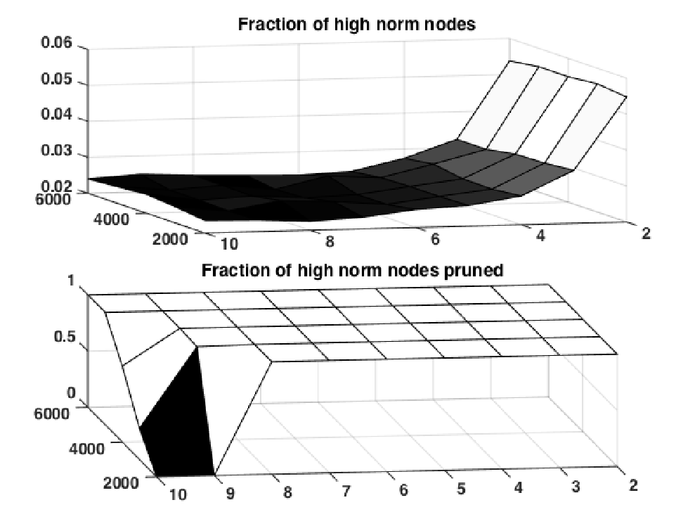
Refer to caption
Figure 5: Top panel: fraction of nodes with high norm. Bottom panel: fraction of nodes with high norm pruned. We vary K∈{2,…,10}K\in\{2,\dots,10\} on the X axis and vary n∈{2000,3000,…,6000}n\in\{2000,3000,\dots,6000\} on the YY axis.

We consider K∈{2,…,10}K\in\{2,\dots,10\} and n∈{2000,3000,…,6000}n\in\{2000,3000,\dots,6000\}, 𝜶=𝟏K/K{\bm{\alpha}}={\bf 1}_{K}/K, 𝐁i​i=1,𝐁i​j=0.001{\bf B}_{ii}=1,{\bf B}_{ij}=0.001 and ρ=log⁡n/n\rho=\log n/n. For each combination we use ϵ\epsilon as the median of the row-wise difference of the empirical eigenvectors from their suitably rotated population counterpart. Let y=maxi⁡‖𝐕i‖y=\max_{i}\|{\bf V}_{i}\| denote the largest row-wise norm of the population eigenvectors; recall that this occurs at one of the corners of the simplex. Let S0S_{0} denote the set of nodes with high empirical eigenvector row-norms (the “high-norm” nodes), defined as S0:={i:‖𝐕^i‖≥y+ϵ}S_{0}:=\{i:\|\hat{\bf V}_{i}\|\geq y+\epsilon\}. SPA will choose at least one of these nodes (and possibly several of them) as its estimated corners. Let B⁡(x,ϵ)B(x,\epsilon) denote the ℓ2\ell_{2} ball of size ϵ\epsilon centered at point xx. For each of the KK corners cic_{i} of the population simplex (cic_{i} equals some row of 𝐕P{\bf V}_{P}), we compute the number of neighborhood points xi:=|{j|𝐕^j∈B⁡(ci,ϵ)}|x_{i}:=|\{j|\hat{\bf V}_{j}\in B(c_{i},\epsilon)\}|; let δ:=mini⁡xi\delta:=\min_{i}x_{i} be the minimum neighborhood size among these corners. Similarly, for each i∈S0i\in S_{0}, we compute zi=|{j|𝐕^j∈B⁡(𝐕^i,ϵ)}|z_{i}=|\{j|\hat{\bf V}_{j}\in B(\hat{\bf V}_{i},\epsilon)\}|. Now we count the fraction of nodes in S0S_{0} that could be pruned without pruning the corners cic_{i} of the population simplex. This fraction is m=∑i∈S0𝟏{zi<δ}|S0|m=\frac{\sum_{i\in S_{0}}{\bf 1}\{z_{i}<\delta\}}{|S_{0}|}. Fig 5 shows that for almost all combinations of KK and nn, we have m=1m=1, i.e., all the nodes in S0S_{0} do get pruned, except for K=10,n=2000K=10,n=2000. This is expected, since for large KK and small nn the pure node density around the corners of the population simplex will be small. Fig 5 shows the fraction |S0|/n|S_{0}|/n of high-norm nodes. For all (K,n)(K,n) combinations pruning removes about a 2% to 6% of the nodes.

Appendix K Extra simulation results

Refer to caption Refer to caption
(i) (ii)
Figure 6: Error against ϵ\epsilon: we use 𝐁i​i=1{\bf B}_{ii}=1, 𝐁i​j=ϵ{\bf B}_{ij}=\epsilon for i≠ji\neq j. (i) K=3K=3. (ii) K=7K=7.

Changing 𝐁{\bf B}: In Fig 6 (i), we plot the relative error in estimating 𝚯{\bm{\Theta}} against increasing off diagonal noise ϵ\epsilon of 𝐁{\bf B}. We take K=3K=3, ρ=0.15\rho=0.15, αi=3/K=1\alpha_{i}=3/K=1, 𝐁i​i=1{\bf B}_{ii}=1, i∈[K]i\in[K]. We see that SPACL outperforms SAAC, SVI, and OCCAM over the entire parameter range. For large ϵ\epsilon, it is also better than GeoNMF and BSNMF.

We also include simulation results with K=7K=7. We take ρ=0.15\rho=0.15, αi=3/K=3/7\alpha_{i}=3/K=3/7, 𝐁i​i=1{\bf B}_{ii}=1, i∈[K]i\in[K]. We see in Fig 6 (ii) that SAAC performs poorly, and OCCAM performs similarly with SPACL, which can also be implied from the simulation results on changing KK. SPACL is more stable and outperforms GeoNMF and BSNMF.