Basic Concepts Involved in Tropical Cyclone Boundary Layer Shocks
ABSTRACT
This paper discusses some basic
concepts that arise in the study of the tropical cyclone frictional boundary
layer. Part I discusses the concepts of asymptotic triangular waves
and asymptotic N-waves in the context of the nonlinear advection equation
and Burgers’ equation. Connections are made between triangular waves
and single eyewalls, and between N-waves and double eyewalls. In Part II,
analytical solutions of a line-symmetric, -plane, slab model of the
atmospheric boundary layer are presented. The boundary layer flow is
forced by a specified pressure field and initialized with and
fields that differ from the steady-state Ekman solution. With certain
smooth initial conditions, discontinuities in and can be produced
during the transient adjustment to the steady-state Ekman solution.
Associated with these discontinuities in the horizontal wind components
are singularities in the boundary layer pumping and the boundary layer
vorticity, which can be either divergence-preferred or vorticity-preferred.
These models serve as a prototype for understanding the role of the
atmospheric boundary layer in the dynamics of primary and secondary
eyewalls in tropical cyclones.
Contents
- I.
Advection Equation and Burgers’ Equation
- 1.
Introduction
- 2.
Asymptotic triangular waves and their conceptual connection with primary eyewalls
- 3.
Asymptotic N-waves and their conceptual connection with moats and double eyewalls
- 3a.
Undamped N-waves
- 3b.
Damped N-waves
- 3a.
- 4.
Triangular waves and primary eyewalls from Burgers’ equation
- 5.
N-waves, moats, and double eyewalls from Burgers’ equation
- 6.
Axisymmetric shocks
- 1.
- II.
Line-Symmetric Slab Ekman Layer Model
- 7.
Analytical solutions for -independent shocks
- 8.
Alternative derivation of the and solutions
- 9.
Examples with initial divergence only
- 9a.
Formation of a triangular wave
- 9b.
Formation of an N-wave
- 9a.
- 10.
Examples with initial vorticity only
- 10a.
Formation of a triangular wave
- 10b.
Formation of an N-wave
- 10a.
- 11.
Concluding remarks
- 7.
I. Advection Equation and Burgers’ Equation
1 Introduction

The NOAA WP-3D aircraft data obtained in Hurricane Hugo (1989) alerted the tropical cyclone research community to the dangers of the tropical cyclone boundary layer and led to research into the possibility that discontinuities (or shocks) in the boundary layer radial and tangential flow can occur in intense hurricanes. This data, which has been discussed in detail by Marks et al. (2008), is reproduced here as Fig. 1. As the aircraft flew at m northeastward towards the eye, the boundary layer tangential wind (solid red curve in the upper panel) increased from 50 m s-1 near km to a maximum of 88 m s-1 near km. At the inner edge of the eyewall, there were multiple updraft-downdraft couplets (the strongest updraft just exceeding 20 m s-1) with associated oscillations of the boundary layer radial and tangential velocity components and a very rapid 60 m s-1 change in tangential velocity near km. After ascending in the eye, the aircraft departed the storm at m (i.e., above the frictional boundary layer), obtaining the horizontal and vertical velocity data shown by the blue curves in Fig. 1. If the tangential wind at m is assumed to be close to gradient balance and the pressure gradient in the boundary layer is essentially the same as that at m, then the region km has supergradient boundary layer flow, while the region km has subgradient boundary layer flow. This is a telltale sign of the importance of the nonlinear advective effects that produce the near discontinuities in and at km and the near singularity in at km.
After the Hugo flight, the risks involved in boundary layer penetrations into the core of intense hurricanes became more fully appreciated, causing NOAA to effectively abandon such penetrations after 1989. However, flights above the boundary layer continued to expand our knowledge of the wind and thermal structure of intense hurricanes. For example, Fig. 2 shows NOAA WP-3D aircraft observations of radar reflectivity and radial profiles of tangential wind, temperature, and dewpoint temperature for Hurricane Frances during a hour interval on 30 August 2004, when the storm was passing just north of the Virgin Islands. This hurricane, described in detail by Rozoff et al. (2008), originated as an African easterly wave that, on 28 August, developed into a major hurricane with a minimum sea-level pressure of 948 hPa and a maximum wind speed of 60 m s-1. During the time interval shown in Fig. 2, Frances had well-defined concentric eyewalls, with a 30 km diameter inner eyewall and a 100 km diameter outer eyewall. Temperatures near the center were as much as C warmer than at radii of 60–70 km, with Fig. 2f showing a warm-ring structure just inside the inner eyewall. In the subsiding air of the echo-free moat between the concentric eyewalls, dewpoint depressions as large as C were observed. Understanding the formation and evolution of such concentric eyewalls is presently an area of active research, with the boundary layer playing an important role in the organization of the moist convection.


We shall argue here that the remarkable convective organization in hurricanes like Hugo and Frances is primarily due to boundary layer dynamics, in particular to the formation of discontinuities in the boundary layer radial inflow and hence singularities in the boundary layer pumping. In terms of the axisymmetric form of the slab boundary layer approximation, tropical cyclone boundary layer dynamics can be described by
| (1) |
where is the radial component, the tangential component, the wind speed, and where the Coriolis parameter , the boundary layer depth , the drag coefficient , and the horizontal diffusivity are assumed to be constants. The specified forcing term can also be interpreted as a specified gradient wind, since the gradient wind is defined in terms of the boundary layer density and pressure by . Slocum et al. (2014) presented three numerical experiments with a slightly generalized version of the slab boundary layer equations (1). Their generalized version includes vertical advection terms and an empirical relation for as a function of . Their specified forcing is shown in the lower panel of Fig. 3, with the associated relative vorticity shown in the upper panel. All three forcing profiles have the same and the same for km. For experiments C1 and C2, the profiles have been locally ( km) enhanced over that of experiment C3 so that the associated profiles differ for km. The sequence C3C2C1 can be considered as an enhancement of the outer gradient balanced flow while the inner core balanced flow remains unchanged. For each of these three specified forcing functions, the numerical model was integrated until a steady state was obtained. Such steady states are generally obtained quickly with most of the change from the initial conditions and occurring in the first hour and only small changes occurring after 3 hours. Figure 4 shows the steady-state boundary layer flows beneath each of these three forcing functions. The three panels show radial profiles ( km) of the boundary layer radial wind (top panel), tangential wind (middle panel), and vertical velocity (bottom panel). Note that in each case, strong radial inflow, supergradient or subgradient tangential winds, and large boundary layer pumping develop. Due to the term in the radial equation of motion, Burgers’ shock-like structures develop just inside the local maxima in the initial tangential wind. At the inner eyewall ( km), the maximum radial inflows are 22 m s-1 for case C3, 11.5 m s-1 for case C2, and 12.5 m s-1 for case C1, so the strength of the inner eyewall shock is considerably reduced by the presence of an outer shock. Note that, even though cases C1 and C2 have stronger inflow than case C3 at km, the situation is reversed at km, a radius at which the radial inflow has been reduced to essentially zero for cases C1 and C2. Although the radial inflows for cases C1 and C2 do somewhat recover in the moat region between the two eyewalls ( km), the width of the moat and the strength of the agradient term are not large enough to allow a full recovery of the radial inflow, leading to an inner eyewall boundary layer pumping (bottom panel of Fig. 4) that is reduced to approximately 50% of the value obtained in case C3. In sections 2--5, the general structure of the radial flow and boundary layer pumping will be related to simple solutions of the nonlinear advection equation and Burgers’ equation. In sections 2 and 4, it will be shown that the radial inflow in case C3 resembles an asymptotic triangular wave, while in sections 3 and 5 it will be shown that the radial inflows in cases C1 and C2 resemble an asymptotic N-wave.11 1 Although the term “inverted N-wave” may be more precise, we use the generic term “N-wave” throughout the discussion here.
This paper is organized into two parts. Part I discusses analytical solutions of the nonlinear advection equation for asymptotic triangular waves (section 2) and asymptotic N-waves (section 3). These two sections review the concepts of hyperbolic equations, the method of characteristics, expansive and compressive regions, wave breaking, multivalued solutions, and the introduction of shock conditions to guarantee single-valued solutions. Sections 4 and 5 discuss the analogous solutions for Burgers’ equation that can be solved analytically via the Cole–Hopf transformation. Since Burgers’ equation includes the horizontal diffusion term, multivalued solutions do not arise, so shock conditions are not required. However, for small values of the diffusion coefficient, the asymptotic triangular wave and the asymptotic N-wave closely resemble those for the advection equation. Sections 2–5 treat line-symmetric problems in the Cartesian coordinate and might be called “toy models” or “metaphors” for certain aspects of tropical cyclone boundary layer dynamics. They are presented here to help understand the boundary layer inflow features that are associated with the advection and diffusion terms in (1). In section 6, we consider analytical solutions of Burgers’ equation for the case of circular symmetry. This axisymmetric case provides further insight into the formation, propagation, and merger of tropical cyclone boundary layer shocks. Part II (sections 7–10) discusses analytical solutions of the line-symmetric version of (1), thus illustrating how multivalued boundary layer solutions can appear in finite time and how the singularities can be either divergence-preferred or vorticity-preferred. The analytical solutions are used to better understand the role of boundary layer shocks in tropical cyclone dynamics. Section 11 presents some concluding remarks, including the implications of the present work on understanding eyewall replacement cycles.
2 Asymptotic triangular waves and their conceptual connection with primary eyewalls
We begin our analysis with the one-dimensional, nonlinear advection problem
| (2) |
where the initial condition is a specified function. In this section, we assume that has the constant value for and , and has values for . Our example assumes , so we are envisioning a boundary layer inflow toward a cyclone center that lies to the left. In our discussion of the asymptotic behavior of the solutions of (2), we shall not be concerned with the details of in the region , but rather only with the fact that in this region. As will be seen, the details of are forgotten as the solution evolves and only the constant and the initial integrated momentum anomaly are remembered at large times.
In order to anticipate some of the discussion to follow, it is interesting to note that is a solution of the nonlinear advection equation with denoting a positive constant. When , we have and the field is steepening with time, i.e., as . In contrast, when , we have and the field is flattening with time, i.e., as . As we shall see below, we need to fit together these two types of solutions and ensure that the result is not multivalued. This gives rise to the concepts of asymptotic triangular waves (this section) and asymptotic N-waves (next section).
Problem (2) is a hyperbolic equation that can also be stated in the characteristic form
| (3) |
where is the derivative along a characteristic. Since it follows from (3) that is invariant along a characteristic and that the characteristics are therefore straight lines in the -plane, the solution is
| (4) |
where is the label (i.e., the initial position) of the characteristic that goes through the point . The continuous solution (4) is valid only until the shock formation time, after which the discontinuity in the solution needs to be tracked via a shock-fitting procedure.

If the shock position at time is denoted by , then from the second part of (4) we obtain
| (5) |
where and are the values of on either side of the shock at time . Elimination of between the two equations in (5) yields
| (6) |
This is one relation between , , and the specified initial condition . A second relation can be found from Whitham’s equal area property, which can be illustrated as follows (Whitham 1974). For the given time , place the points and on the curve shown in Fig. 5. According to the equal area property, these two points will simultaneously reach the shock at time if the secant line between them cuts off equal areas of the curve. This equal area property can be expressed as
| (7) |
As time proceeds, decreases and eventually becomes less than , after which and the lower limit of the integral in (7) can be set to . Equations (6) and (7) then simplify to
| (8) |
| (9) |
Eliminating between these last two equations, we obtain
| (10) |
As time proceeds further, increases and eventually reaches zero, after which, equation (10) yields
| (11) |
where the initial integrated momentum anomaly is defined by
| (12) |
From (4) and (11), we obtain the asymptotic formula
| (13) |
for the value of just behind (i.e., just to the right of) the leftward-moving shock. From (5), the asymptotic form of the shock position is
| (14) |
Therefore, the asymptotic form of the solution is
| (15) |
which is a triangular wave as plotted in Fig. 6. The jump in across the shock is and the width of the triangular region behind the shock is , so the area under the curve remains equal to its initial value . Since the asymptotic formula (15) involves only and , the details of the initial condition are lost. The region where might be called the “forgetful region.” To summarize, all initial conditions with the same and have the same ultimate behavior. A smooth initial pulse of radial inflow evolves into an asymptotic triangular wave, with a discontinuity in the radial velocity and a singularity in the boundary layer pumping. This is conceptually similar to the profile of case C3 in the top panel of Fig. 4.
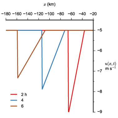
3 Asymptotic N-waves and their conceptual connection with moats and double eyewalls
a Undamped N-waves
In the previous section, we presented some ideas concerning the question of how a smooth pulse of enhanced radial inflow evolves into a primary eyewall shock. We now consider the following related question: How does a smooth undulation of enhanced and reduced radial inflow evolve into double eyewall shocks? The initial condition for this section is illustrated in the upper panel of Fig. 7. Since there are two compressive regions where surrounding a single expansive region where , we expect two shocks to form. The initial integrated momentum anomalies for the forward and rear areas are defined by
| (16) |
where is the left enhanced area and is the right reduced area. The characteristics for this problem are shown in the lower panel of Fig. 7 and the asymptotic solution is given by
| (17) |
which is an N-wave as plotted in Fig. 8 for m s-1 and h. Figure 8a is for the choice m2 s-1, which produces forward and rearward shocks of equal strength. Figure 8b is for the choice m2 s-1 and m2 s-1, which produces a rearward shock that is weaker than the forward shock. The jump in across the front shock is , while the jump across the rear shock is . The width of the region between the two shocks is . The area under the curve in the left portion of the N-wave remains equal to its initial value of , while the area under the curve in the right portion of the N-wave remains equal to its initial value of .


This N-wave pattern for the nonlinear advection equation is similar to the N-wave patterns shown in the top panel of Fig. 4 for the slab boundary layer model simulations of concentric eyewalls (cases C1 and C2).
b Damped N-waves
This section discusses how initial conditions that result in two shocks (i.e., N-waves) in the undamped problem (2) can lead to two, one, or no shocks in the damped problem. We begin the analysis with the damped nonlinear advection problem
| (18) |
where is the constant damping time scale and the initial condition is a specified function. Problem (18) is a hyperbolic equation that can also be stated in the characteristic form
| (19) |
where is the derivative along a characteristic. Since is invariant along each characteristic, the solution of the first equation in (19) is
| (20) |
where is the label (i.e., the initial position) of the characteristic that goes through the point . Using the solution (20) in the right-hand side of the second equation in (19) and then integrating in time, we obtain
| (21) |
The characteristics defined by (21) are not straight lines in the -plane, although they do become straight in the limit , in which case . If shocks appear, the continuous solution (20) and (21) is valid only until the first shock formation time, after which the discontinuity in the solution needs to be tracked via a shock-fitting procedure. The vertical motion implied by the solution can be found from , where the boundary layer depth is taken as 1000 m. Using (20) and (21), we obtain the boundary layer pumping formula
| (22) |
where is the first derivative of the initial condition . A singularity in will occur along the characteristic if and when , i.e., at the shock formation time given implicitly by
| (23) |

| Case | |||||
|---|---|---|---|---|---|
| (h) | (h) | (h) | |||
| A | 0.05 | 3.33 | 0.150 | 3.03 | 4.96 |
| B | 0.05 | 2.22 | 0.225 | 5.01 | No Shock |
| C | 0.05 | 1.67 | 0.300 | No Shock | No Shock |
| D | 0.00 | 3.33 | 0.150 | 3.05 | 3.05 |
| E | 0.00 | 1.67 | 0.300 | No Shock | No Shock |

As an example, consider the initial condition
| (24) |
where the initial maximum flow , the horizontal scale , and the asymmetry parameter are specified constants. Plots of (24) for are shown in Fig. 9. Note that, when , the field is perfectly anti-symmetric about . Since the derivative of (24) is
| (25) |
it is easily seen that the minimum value of occurs at and the maximum value occurs when , with the corresponding values of being and , respectively. The second derivative of (24) is
| (26) |
From the numerator on the right-hand side of (26), we see that at and at the two points that are solutions of the quadratic equation . These two solutions, denoted by and , are
| (27) |
The points and correspond to local minima of , while the point corresponds to a local maximum of . A shock cannot occur along the characteristic because and cannot ever be satisfied. However, shocks can occur along the characteristics and . We denote the shock formation time along these two characteristics as and . From (23) and (25), we then obtain
| (28) |
where
| (29) |
for . Solving (28) for , we obtain
| (30) |
This formula has been used to construct Fig. 10, which divides the dimensionless -plane into three regions. In the hatched region, two shocks occur since the argument of the natural logarithm in (30) is positive for both and . The shock formation time for the left shock occurs before the right shock for initial conditions where . In the blue region, a shock occurs only on the left side since the argument of the natural logarithm is positive only for . In the white region, no shocks occur since the argument of the natural logarithm is negative for both and . Table 1 lists data for the five examples indicated by the dots A–E in Fig. 10. The solutions at three different times are plotted22 2 In order to avoid iterative procedures in dealing with the implicit nature of the solutions (20)–(21), a simple way to produce plots of these solutions is as follows. Choose a time and then calculate the corresponding from the second entry in (21). Choose a set of equally spaced values of and then use the first entry in (21) to calculate the corresponding set of unequally spaced values of . Then use (20) to calculate at the unequally spaced -points. Finally, plot as a function of at the chosen time using a plotting routine that can handle unequally spaced data points. in Fig. 11. For the cases that produce one or two shocks (cases A,B,D), the final time is the shock formation time for the left shock (between 3 and 5 hours, as listed in Table 1). For the cases that don’t produce a shock (cases C and E), the times are 0, 3, and 6 h. Note that all cases are characterized by a broadening divergent region with collapsing convergent regions on each side. Cases A and D have weak damping ( h) and produce two shocks, while cases C and E have strong damping ( h) and do not produce shocks. Case B has an intermediate value of damping ( h) and produces a shock only on the left side. Another view of cases A and C is provided by the characteristic curves shown in Fig. 12. The upper panel (case A) illustrates the intersection of characteristics on the left side near h. In the lower panel (case C), the damping is strong enough that no shocks are produced, even though there is some concentration of convergence on the left side.


4 Triangular waves and primary eyewalls from Burgers’ equation
To further understand the formation and propagation of boundary layer shocks, we now consider Burgers’ equation
| (31) |
with the initial and boundary conditions
| (32) |
where the function and the constant are specified. For ease of physical interpretation, we again assume that , i.e., a basic inflow toward the storm center, which lies far to the left of the origin. Note that the Burgers’ equation (31) captures three important terms in the radial momentum equation of the slab boundary layer model (1), albeit in the line-symmetric rather than the axisymmetric form. An excellent general mathematical discussion of Burgers’ equation can be found in the book by Whitham (1974).
In sections 2 and 3, the discussion concerned solutions of the hyperbolic problems (2) and (18), so that the method of characteristics played a central role. Since Burgers’ equation (31) is not hyperbolic, the method of characteristics is not useful. However, considerable analytical progress can be made using the Cole–Hopf transformation. The mathematical analysis given here follows that given by Lighthill (1956) in his study of viscosity effects in sound waves of finite amplitude. Although our application to the radial inflow in the tropical cyclone boundary layer has nothing to do with compressibility effects and finite amplitude sound waves, we have adapted Lighthill’s mathematical analysis to our problem. We begin by considering solutions of Burgers’ equation with an initial condition consisting of a localized irregularity superposed on the constant flow . Define the new dependent variable and the new independent variables . Then
| (33) |
and Burgers’ equation becomes
| (34) |
with the initial and boundary conditions
| (35) |
An integral relation associated with the problem (34)–(35) can be obtained by writing (34) in the form
| (36) |
and then integrating over the entire domain to obtain the conservation relation , where
| (37) |
so that the integrated momentum is an invariant of the problem.
The problem (34)–(35) can be solved analytically using the Cole–Hopf transformation. The first step in this transformation is to use (36) to define the velocity potential such that
| (38) |
Combining these last two equations, we obtain
| (39) |
The second step in the Cole–Hopf transformation is to define the new dependent variable by
| (40) |
from which it follows that
| (41) |
| (42) |
with the initial and boundary conditions
| (43) |
where is the Reynolds’ number. Thus, the Cole–Hopf procedure (38)–(41) has transformed the nonlinear advection-diffusion equation (34) to the linear diffusion equation (42). If we can solve the diffusion equation (42) for , we can recover the solution of the nonlinear equation (34) from
| (44) |
The challenge now is to find a simple solution of (42) and (43) that translates into a physically interesting solution of (31) and (32).
An interesting solution of the diffusion equation (42) is
| (45) |
where the complementary error function is given in terms of the error function by
| (46) |
To verify that the boundary conditions in (43) are satisfied, note that as , and that as . The diffusion equation solution (45) is shown in the top panel of Fig. 13, where is plotted as a function of for the three Reynolds’ numbers .
Using (45) in (44), we obtain the Burgers’ equation solution
| (47) |
Translating back to the original variables, the solution (47) can be written in the form
| (48) |
One way to display the solution (48) is to plot as a function of . This is shown in the bottom panel of Fig. 13 for the three different Reynolds’ numbers . A more physically intuitive way to display the solution (48) is to plot for the choices m s-1, m2 s-1, and . This is shown in the top panel of Fig. 14 for h. If is interpreted as the divergent component of the flow in a slab boundary layer of constant depth , then the implied boundary layer pumping is given by . Profiles of at h are shown in the bottom panel of Fig. 14, assuming m. As discussed in section 2 for the advection equation (see Fig. 6), the shock strength decreases as while the width of the subsidence region increases as . It is worth noting that if is increased, we will retrieve the asymptotic solutions shown in Fig. 6 and that if decreases, the diffusion would increase and smooth the discontinuity as shown in Fig. 13. The smoothing of the discontinuity in the field as decreases represents a “shock-like” feature.


5 N-waves, moats, and double eyewalls from Burgers’ equation
The diffusion equation solution (45) gives rise to the triangular wave solution (48). Another interesting diffusion equation solution gives rise to an N-wave solution. This diffusion equation solution is
| (49) |
where the constant is determined below. Using the diffusion equation solution (49) in (44), we obtain the Burgers’ equation solution
| (50) |
The integrated momentum excess in the region is defined by
| (51) |
where the second equality follows from (44) and the third equality from (49). This is also equal to the integrated momentum deficit in the region as given by
| (52) |
The effective Reynolds’ number is defined by
| (53) |
so that the value of at is given by and the constant can be expressed in terms of by . Using this last relation, the solution (50) can be written in the form
| (54) |
Translating back to the original variables, we obtain
| (55) |
which is plotted in Fig. 15a for h.
In order to compare the solution (55) to the solution (17) of the nonlinear advection equation in section 3, consider the case where , in which case (55) becomes
| (56) |
For this case of , in the region , the exponential term in (56) can be neglected so that , while in the region , the exponential term is much greater than unity so that . Thus, the solution is
| (57) |
when becomes large.
As before, if is interpreted as the divergent component of the flow in a slab boundary layer of constant depth , then the implied boundary layer pumping is given by , which is plotted in Fig. 15b for h. Since the integrated momentum deficit in the region is equal to the integrated momentum excess in the region , this example produces shocks of equal strength on the leading and trailing edges of the widening moat. Examples with shocks of unequal strength are also possible and examples with the stronger shock on the leading edge more closely resemble what happens in hurricanes with concentric eyewalls.

The simple Burgers’ equation solutions discussed here can serve as the basis of the following conjecture. When an anomaly forms in the boundary layer radial inflow, it tends to evolve into either a broadening triangular wave pattern with concentrated Ekman pumping on the inner edge or a broadening N-wave pattern with concentrated Ekman pumping on both sides of a moat region with weak subsidence. In other words, a single eyewall is formed when the term distorts the boundary layer radial inflow into a triangular wave, while concentric eyewalls are formed when the inflow is distorted into an N-wave.
6 Axisymmetric shocks
In the previous two sections, we have studied solutions of the Cartesian coordinate form of Burgers’ equation. In this section, we shift our attention to the polar coordinate form
| (58) |
which can also be solved analytically using the Cole–Hopf transformation. In particular, the Cole–Hopf transformation of the nonlinear, advection-diffusion equation (58) leads to the linear diffusion equation (64). An integral representation of the solution to (64) is given by (71), where is defined by (73). When this diffusion equation solution is translated back to the Burgers’ equation solution , one obtains (74). Since the Burgers’ equation solution (74) is expressed as the ratio of two integrals, its detailed structure is difficult to see, although the application of asymptotic methods (not discussed here) can reveal certain aspects of the solution structure. Because of the mathematical details involved here, some readers may wish to skip directly to section 7, simply noting that the polar coordinate version (58) of Burgers’ equation can indeed be solved by the Cole–Hopf transformation.
To proceed with the details of the Cole–Hopf transformation, the first step in the transformation is to write (58) in the form
| (59) |
and then to define the velocity potential such that
| (60) |
Combining these last two equations, we obtain
| (61) |
The second step in the Cole–Hopf transformation is to define the new dependent variable by
| (62) |
from which it follows that
| (63) |
| (64) |
Thus, the Cole–Hopf procedure has transformed the nonlinear advection-diffusion equation (58) to the linear diffusion equation (64). If we can solve the diffusion equation (64) for , we can recover the solution of the nonlinear equation (58) from
| (65) |
If is interpreted as the divergent component of the flow in a slab boundary layer of constant depth , then the implied boundary layer pumping is given by
| (66) |
In the remainder of this section, we derive solutions of (64) from which we obtain the corresponding and fields.
Solutions of (64) can be found by a variety of methods, one of which is the Hankel transform method. The Hankel transform pair is
| (67) |
| (68) |
where is the order zero Bessel function and is the radial wavenumber. Multiplying (64) by , integrating over all , performing integration by parts twice using the Bessel function derivative formulas and , we can transform the partial differential equation (64) into the ordinary differential equation
| (69) |
The solution of (69) is
| (70) |
where the second equality follows from the use of (67) at . Substituting (70) into (68) yields
| (71) |
where
| (72) |
We next make use of Weber’s second exponential integral, which is given on page 393 of Watson (1995) and on page 739 of Gradshteyn and Ryzhik (1994). This allows us to write (72) as
| (73) |
where is the order zero modified Bessel function. The second line in (73) is a useful form for because as .
Equation (71) gives the solution for the diffusion problem (64). The solution of the original problem (58) is then found by substituting (71) into (65), which yields
| (74) |
where denotes the partial derivative of with respect to . Note that in the relation (73) for , and thus in (71) for , the constant always appears coupled to , i.e., only as the product . This is not a property of the solution (74). In fact, the field diffuses while the field shocks.
As a simple example, choose the initial field to be
| (75) |
where are constants. The exponents in (75) define two Reynolds’ numbers as and . For example, if km, m s-1, km, m s-1, and m2 s-1, we have and . Using (62), the corresponding initial field is
| (76) |
and, from the first entry in (60), the corresponding initial field is
| (77) |
For reasonable choices such as and , this example illustrates a simple boundary layer mechanism for the merging of tropical cyclone convective rings into a single eyewall structure. In other words, the solution (74) can describe the merger of two shocks that propagate inward. As the outer shock overtakes the inner one, the details of the evolving structure are lost and a very simple final shock-like structure is obtained. A thorough examination of such solutions is left for future study.
We conclude Part I by asking: “How do hurricane eyewalls originate?” The results of sections 2 and 4 suggest the possibility that a single eyewall is a phenomenon instigated by the tendency of the boundary layer radial inflow to form a single shock on the inward edge of a region of enhanced radial inflow. Similarly, the results of sections 3 and 5 suggest the possibility that a double eyewall is a phenomenon instigated by the tendency of the boundary layer radial inflow to form a double shock (or N-wave) on the inward and outward edges of a region that has both enhanced and reduced radial inflow. In either case, the formation of a boundary layer shock may be one of the most important events in the life cycle of a hurricane, for it imposes on the storm a classic eye/eyewall structure. In comparing our solutions to observed aspects of the tropical cyclone boundary layer, we note that these solutions lack the pressure gradient force and dissipative effects. The result is that we capture only some of the evolution seen in nature.
II. Line-Symmetric Slab Ekman Layer Model
7 Analytical solutions for -independent shocks
We now return to the discussion of the slab boundary layer model (1). In the absence of horizontal diffusion, the line-symmetric version of (1) can be solved analytically using the method of characteristics. Thus, consider the line-symmetric slab boundary layer equations
| (78) |
where is the wind speed, and where the Coriolis parameter , the boundary layer depth , and the drag coefficient are assumed to have the values s-1, m, and . The forcing term , which is also assumed to be a constant, can be interpreted in terms of a specified geostrophic wind , since . Our goal is to solve the system (78) for and on an infinite domain subject to the initial conditions
| (79) |
where and are specified functions. Obviously, the line-symmetric boundary layer dynamics (78) lacks important curvature effects and misses important spatial variations to the forcing that are present in the axisymmetric dynamics (1). Thus, (78) should be regarded as a qualitative model of the hurricane boundary layer. Its attraction is the ease with which analytical solutions can be obtained for a coupled pair of equations that increases our understanding of shocks in the full slab model (1).
The quasi-linear system (78) is hyperbolic and can be written in characteristic form, i.e., it can be written as a system of ordinary differential equations. In order to make the characteristic form of the and equations homogeneous, it is convenient to introduce the constant Ekman flow components and , which are determined from the nonlinear algebraic system
| (80) |
where . The “solutions” of (80) are
| (81) |
These two relations are implicit because the wind speed depends on the velocity components and . However, we can find an explicit solution for by squaring each equation in (81) and adding the results to obtain
| (82) |
where and . Equation (82) can be solved as a quadratic for , yielding33 3 Note that can be interpreted as the “slab Ekman number,” i.e., as the ratio of the magnitudes of the drag force and the Coriolis force. Similarly, can be interpreted as the “forced Ekman number.”
| (83) |
For the five values of listed in the first column of Table 2, the second column lists the corresponding values of , the third column lists the corresponding values of determined from (83), while the fourth and fifth columns list the corresponding values of and determined from (81).
| (m s-1) | (m s-1) | (m s-1) | ||
|---|---|---|---|---|
| 10 | 0.4 | 0.3746 | 8.77 | |
| 20 | 0.8 | 0.6659 | 13.86 | |
| 30 | 1.2 | 0.8944 | 16.67 | |
| 40 | 1.6 | 1.0846 | 18.38 | |
| 50 | 2.0 | 1.2496 | 19.52 |

We now approximate the factors in (78) by . Then, combining this approximate form of (78) with (80), we obtain the characteristic form
| (84) |
where can be interpreted as the derivative along a characteristic. In the special case , the two momentum equations in (84) decouple, and the first reduces to the nonlinear advection equation with damping, which was discussed in section 3b. Thus, we anticipate the possible appearance of shocks in the solutions of the coupled equations (84). As can be checked by direct substitution, the solutions of the coupled and equations in (84) are
| (85) |
| (86) |
where is the initial position of the characteristic. According to (85) and (86), if and/or , there will be damped inertial oscillations along each characteristic, leading to eventual steady-state Ekman balance. To find the shapes of the characteristics, we now substitute the solution for into the right-hand side of , and then integrate from zero to along a characteristic, thereby obtaining
| (87) |
where the and functions are defined by
| (88) |
To verify that (87) and (88) constitute a solution of , take of (87) and make use of and . Plots of and for the cases ( m s-1) and ( m s-1) are shown in the two panels of Fig. 16. Since each characteristic can be considered to be uniquely labeled by its value of , equations (85) and (86) give the variation of and along the characteristic, while (87) gives the shape of the characteristic. Thus, (85)–(88) constitute the solution of the original problem (78) and (79), with the understanding that the factors in (78) have been approximated by , and the solution does not extend past shock formation time.44 4 In analogy with the procedure used in section 3, iterative calculations can be avoided in dealing with the implicit nature of the solutions (85)–(88) by producing plots of these solutions as follows. Choose a time and then calculate the corresponding and from (88). Choose a set of equally spaced values of and then use (87) to calculate the corresponding set of unequally spaced values of . Then use (85) and (86) to calculate and at the unequally spaced -points. Finally, plot and as functions of at the chosen time using a plotting routine that can handle unequally spaced data points.
To understand when the divergence and the vorticity become infinite, we first note that of (87) yields
| (89) |
so that of (85) and (86) yield
| (90) |
From the analytical solutions (90), we can easily obtain
| (91) |
To compute the time of shock formation, we note that, from the denominators on the right-hand sides of (90), the divergence and the vorticity can become infinite if
| (92) |
along one or more of the characteristics. Note from Fig. 16 that the values of and may never get large enough to satisfy (92), in which case a shock will not form. In section 9 we consider shock formation for initial conditions with and , while in section 10 we consider initial conditions with and . However, before discussing these particular initial conditions, we provide in section 8 an alternative derivation of the solutions (90).
8 Alternative derivation of the and solutions
Since it is the divergence and vorticity that can become infinite when a shock occurs, rather than the velocity components and , it is of interest to recall the governing equations for and . These equations, derived from (84), can be written as
| (93) |
| (94) |
where we have assumed and . Note that the term in (93) originates from the term in the -momentum equation and that the term in (94) originates from the term in the -momentum equation. Thus, we expect that the and terms play a crucial role in the development of any singularities in divergence and vorticity.
Taking the sum of times (93) and times (94), we obtain
| (95) |
so that decays along a characteristic when and grows along a characteristic when , i.e., growth occurs when the magnitude of convergence exceeds the critical value . If, at any time , the divergence and vorticity satisfy , then it follows that and, according to (95), will further decrease. Thus, a necessary condition for shock formation is .

We now consider the derivation of the solutions for and directly from (93) and (94). As before, let be the label of a given characteristic, with a convenient choice for this label being the initial position of the characteristic. Since the label is invariant along the characteristic, we have . Then, taking of this last relation we obtain
| (96) |
which is an equation relating the spacing of the characteristics to the divergence . Now search for solutions of (93) and (94) having the form
| (97) |
When characteristics come together in the -plane, the dimensionless spacing goes to zero and the above factor goes to infinity. In this way the solutions and can become singular while and remain well-behaved. Substitution of (97) into the divergence equation (93) yields
| (98) |
where the last line follows from the fact that (96) can be used to verify cancellation of the last two terms in the second line. Similarly, substitution of (97) into the vorticity equation (94) yields
| (99) |
where, as before, the last line follows from the fact that (96) can be used to verify cancellation of the last two terms in the second line. Thus, while and satisfy the nonlinear equations (93) and (94), the new variables and satisfy the linear equations
| (100) |
The solutions of the coupled equations (100) are
| (101) |
Combining (96), (97), and the first line of (101), it can be shown that
| (102) |
Integrating (102), noting that at , we find that the spacing of the characteristics is given by the inverse of (89), i.e.,
| (103) |
When (101) and (103) are substituted into (97), we recover the previously derived solutions (90) for and and gain insight into the role of the intersection of characteristics in the formation of singularities in and .
9 Examples with initial divergence only
In this section, we consider examples for which there is initial divergence, but no initial vorticity. The initial condition used in section 9a leads to the formation of a triangular wave, or single eyewall structure, while the initial condition used in section 9b leads to the formation of an N-wave, or double eyewall structure. In section 10, we consider examples for which there is initial vorticity, but no initial divergence.
a Formation of a triangular wave

In the first example, consider the initial conditions
| (104) |
where the constants and specify the horizontal extent and strength of this initial symmetric divergent flow anomaly. The initial divergence and vorticity associated with (104) are
| (105) |
We assume so that initially convergence appears to the left of the origin and divergence to the right. With these initial conditions, the solutions (85) and (86) simplify to
| (106) |
while the characteristic equation (87) simplifies to
| (107) |
The solutions (90) for the divergence and vorticity become
| (108) |
so that
| (109) |
From (108) or (109), shock formation occurs along the characteristic when . This occurs first along the characteristic with the minimum value of . For this example, the minimum value of occurs at , so that, from (105), . Application of (109) along the characteristic yields
| (110) |
Thus, the shock formation time is given implicitly by
| (111) |
and, from (107), the position of shock formation is
| (112) |
Note from Fig. 16 that equation (111) has a solution only when is smaller than the maximum value of . The maximum value of occurs at h and, from (88), has the value
Thus, the condition for shock formation is
| (113) |

Equations (111) and (113) have been used to construct the top panel of Fig. 17, which shows isolines of the shock formation time and the shock critical condition (thick line) in the -plane. There is only a weak dependence of on , with shock formation times less than one hour when . The three columns of Fig. 18 show three examples of the analytical solutions (106)–(108). The four rows show plots of , , , and as functions of with the initial conditions given by the gray curves and the distributions at shock formation time given by the red curves (corresponding to 45 min for the left column, 29 min for the middle column, and 22 min for the right column). As the spatial variation of the initial increases, the final jump in also increases, but the final jump in changes little. Since the final jumps in are smaller than the corresponding final jumps in , all three cases can be classified as divergence-preferred triangular waves.
b Formation of an N-wave
For the second example, consider the initial conditions
| (114) |
where the constants and now specify the horizontal extent and strength of this initial antisymmetric divergent flow anomaly. The initial divergence and vorticity associated with (114) are
| (115) |
We assume , which is the case leading to an N-wave and a double shock. With the initial conditions (114), the solutions (85) and (86) become
| (116) |
and the characteristic equation (87) becomes
| (117) |
The solutions (90) for the divergence and vorticity become
| (118) |
so that
| (119) |
From (118) or (119), shock formation occurs along a characteristic when . This occurs first along the two characteristics with the minimum value of the initial divergence , i.e., along the two characteristics with the maximum value of the initial convergence. For this example, the two minimum values of occur at , so that, from (115), . Application of (119) along the two characteristics , where , yields
| (120) |
Thus, the shock formation time is given implicitly by
| (121) |
and, from (117), the positions of shock formation are
| (122) |
From Fig. 16, equation (121) has a solution only when is smaller than the maximum value of . The maximum value of occurs at h and, from (88), has the value
Thus, the condition for shock formation is
| (123) |
Isolines of the shock formation time , as given implicitly by (121), and the shock condition, as given by (123), are shown in the bottom panel of Fig. 17. The solutions for , as given by (116)–(118), are plotted in Fig. 19 for the particular constants m s-1, km, and for the three cases m s-1. All three examples evolve into N-waves in and , and therefore singularities in the Ekman pumping on both edges of the widening moat.
The time evolution of the divergence and vorticity along the shock-producing characteristics for these N-waves is shown by the bluish curves in the lower panel of Fig. 20. All three cases are divergence-preferred, so the discontinuities in are larger than those in .


10 Examples with initial vorticity only
In this section, it is shown that triangular waves and N-waves can also be produced from initial conditions that have zero divergence and nonzero vorticity.
a Formation of a triangular wave
As the first set of simple examples for this section, consider the initial conditions
| (124) |
where the constants and specify the horizontal extent and strength of this initial rotational flow anomaly. The initial divergence and vorticity associated with (124) are
| (125) |
We assume so that negative initial vorticity appears to the left of the origin. With these initial conditions, the solutions (85) and (86) simplify to
| (126) |
while the characteristic equation (87) simplifies to
| (127) |
The solutions (90) for the divergence and vorticity become
| (128) |
so that
| (129) |
From (128) or (129), shock formation occurs along the characteristic when . This occurs first along the characteristic with the minimum value of . For this example, the minimum value of occurs at so that, from (125), . Application of (129) along the characteristic yields
| (130) |
Thus, the shock formation time is given implicitly by
| (131) |
and, from (127), the position of shock formation is
| (132) |
Note from Fig. 16 that equation (131) has a solution only when is smaller than the maximum value of . The maximum value of occurs at h and, from (88), has the value
Thus, the condition for shock formation is
| (133) |

The solutions for , , , and , as given by (126)–(128), are plotted in Fig. 22 for the constants m s-1, km, and m s-1 for cases Aζ, Bζ, and Cζ. The plots cover the spatial interval km and are for and , where h is the shock formation time for each initial condition.
The time evolution of the divergence and vorticity along the first shock-producing characteristic is shown by the reddish curves in the top panel of Fig. 20. Note from (128) that , so that the shock is vorticity-preferred if and is divergence-preferred if . All three of the cases Aζ, Bζ, Cζ fall in the former range and are therefore vorticity-preferred triangular waves.
b Formation of an N-wave

As the second set of simple examples for this section, consider the initial conditions
| (134) |
where the constants and now specify the horizontal extent and strength of this initial anti-symmetric rotational flow anomaly. The initial divergence and vorticity associated with (134) are
| (135) |
We assume , so that negative initial vorticity appears on the wings of a central region of positive vorticity. With these initial conditions, the solutions (85) and (86) simplify to
| (136) |
while the characteristic equation (87) simplifies to
| (137) |
The solutions (90) for the divergence and vorticity become
| (138) |
so that
| (139) |
From (138) or (139), shock formation occurs along a characteristic when . This occurs first along the two characteristics with the minimum value of the initial vorticity . For this example, the two minimum values of occur at , so that, from (135), . Application of (139) along the two characteristics , where , yields
| (140) |
Thus, the shock formation time is given implicitly by
| (141) |
and, from (137), the positions of shock formation are
| (142) |
From Fig. 16, equation (141) has a solution only when is smaller than the maximum value of . The maximum value of occurs at h and, from (88), has the value
Thus, the condition for shock formation is
| (143) |
The solutions for , , , , as given by (136)–(138), are plotted in Fig. 23, using the constants m s-1, 10 km, and m s-1 for cases Dζ, Eζ, Fζ. As can be seen from the lower panel of Fig. 20, the case Dζ produces divergence-preferred N-wave shocks, while cases Eζ and Fζ produce N-wave shocks that are of nearly equal strength in divergence and vorticity.
11 Concluding remarks
In sections 2–6, we have reviewed the theory of the one-dimensional nonlinear advection equation and Burgers’ equation. These two equations provide a simple framework for understanding the concepts of triangular waves and N-waves. In sections 7–10, we have considered the line-symmetric slab boundary layer model (78). Although this model lacks important curvature effects that are present in the axisymmetric slab boundary layer model (1), the line-symmetric model is simple enough for analytical progress and generalization of the concepts of triangular waves and N-waves. In particular, the line-symmetric model (78) has been solved by taking advantage of its hyperbolic form, thereby rewriting it as the system of three ordinary differential equations given in (84). The solutions of these three ordinary differential equations are given in (85)–(88), with the associated divergence and vorticity solutions given in (90). When the denominators on the right hand sides of (90) vanish, the divergence and vorticity become infinite, so there appears a singularity in the boundary layer pumping along with a vertically oriented vorticity sheet in the boundary layer. As shown by the examples in sections 9 and 10, such shocks develop when the initial convergence or initial vorticity exceed a critical value. The shocks can be classified as divergence-preferred or vorticity-preferred, depending on whether the jump in the divergent component is larger than the jump in the rotational component , or vice versa. In this regard it is interesting to note that the classic Hurricane Hugo case (Fig. 1) can be interpreted as a vorticity-preferred shock, with the jump in the rotational component nearly three times as large as the jump in the divergent component.
The plots shown in sections 9 and 10 display the solutions up to the shock formation time . How do we extend the solutions beyond , i.e., into regions of the -plane where characteristics intersect and the solutions (85) and (86) become multivalued? Although the momentum equations (78) remain valid in the smooth regions of flow, these equations are not useful at the discontinuity, where and become infinite. Thus, equations (78) need to be supplemented by jump conditions that describe the dynamics across the shock. One practical alternative to the use of jump conditions is to include horizontal diffusion terms in (78), but to set the diffusivity constant to such a small value that the horizontal diffusion terms have importance only in the region near the shock. Then, since and are prevented from becoming infinite, explicit jump conditions are not required. This strategy of including horizontal diffusion was used in the numerical simulations of single and double eyewalls shown in Fig. 4. Another practical alternative to the use of jump conditions involves shock-capturing numerical methods such as those used by Kuo and Polvani (1997) to simulate the shocks that appear as transient features in the fully nonlinear, shallow-water, geostrophic adjustment problem.
The results presented here provide some insight into questions such as: (1) What determines the size of the eye? (2) How are potential vorticity rings produced? (3) How does an outer concentric eyewall form and how does it influence the inner eyewall? The slab boundary layer results support the notion that the size of the eye is determined by nonlinear processes that set the radius at which the eyewall shock forms. A boundary layer potential vorticity ring is also produced at this radius. By boundary layer pumping and latent heat release, the boundary layer potential vorticity ring is extended upward. If, outside the eyewall, the boundary layer radial inflow does not decrease monotonically with radius, a concentric eyewall boundary layer shock can form. If it is strong enough and close enough to the inner eyewall, this outer eyewall shock can chock off the boundary layer radial inflow to the inner shock and effectively shut down the boundary layer pumping at the inner eyewall. An important issue not explored here is the distinction between weak and strong shocks. Although some initial conditions can technically produce shocks, they may be too weak to be of physical significance. Thus, an interesting remaining problem is to determine the conditions that produce strong enough shocks that the boundary layer can take control of the organization of the deep moist convection in the cyclone.
The frictional boundary layer comprises only about 10% of the mass involved in the tropical cyclone circulation. However, because of its high moisture content and its tendency to produce regions of intense convergence and Ekman pumping, it can dictate the location and strength of primary and secondary eyewalls. Thus, the dynamical importance of the frictional boundary layer far exceeds its fractional mass content. Concerning the location and strength of eyewall convection, the basic idea presented here is that the single and double eyewall structures observed in tropical cyclones are a result of the nonlinear dynamics of the boundary layer. Because of the term in the radial equation of motion, divergent regions of boundary layer flow broaden and weaken with time, while convergent regions sharpen and strengthen with time. Single eyewalls develop when the sharpening process is dominant on the inside edge of the divergent moat, in analogy with the development of a triangular wave. Concentric eyewalls develop when the sharpening process is active on both sides of the moat, in analogy with the development of an N-wave. An interesting aspect of tropical cyclone boundary layer dynamics is that the term in the radial equation of motion can be negligible at most radii, so that a local Ekman theory (i.e., a theory that neglects radial advection) yields a reasonable approximation to the flow at most radii. However, as a tropical cyclone intensifies, there can develop radial intervals where local Ekman theory breaks down and Burgers-type sharpening effects become dominant in determining the boundary layer flow structure. It can be argued that such sharpening processes are crucial in producing the classic single or double eyewall structures that define a hurricane.
In closing we note that the present study has focused on understanding the boundary layer response to a specified, axisymmetric, non-translating pressure field, in which case the boundary layer shocks are circular. Tropical cyclones are rarely stationary, and when the pressure field translates, the boundary layer shocks can form more complicated structures, such as crescent shapes or spiral shapes. Understanding the development of boundary layer shocks forced by a translating pressure field remains a challenging problem.
Acknowledgments.
We would like to thank Alex Gonzalez, Paul Ciesielski, and Gabriel Williams for their advice. This work has been supported by the NSF under Grants AGS-1546610 and AGS-1601623 and by the Hurricane Forecast Improvement Project (HFIP) under NOAA Grant NA090AR4320074.
REFERENCES
- Gradshteyn and Ryzhik (1994) Gradshteyn, I. S., and I. M. Ryzhik, 1994: Tables of Integrals, Series, and Products, 5th edition. Academic Press, 1204 pp.
- Kuo and Polvani (1997) Kuo, A. C., and L. M. Polvani, 1997: Time-dependent fully nonlinear geostrophic adjustment. J. Phys. Oceanogr., 27, 1614–1634.
- Lighthill (1956) Lighthill, M. J., 1956: Viscosity effects in sound waves of finite amplitude. Surveys in Mechanics, G. K. Batchelor, and R. M. Davies, Eds., Cambridge University Press.
- Marks et al. (2008) Marks, F. D., P. G. Black, M. T. Montgomery, and R. W. Burpee, 2008: Structure of the eye and eyewall of Hurricane Hugo (1989). Mon. Wea. Rev., 136, 1237–1259.
- Rozoff et al. (2008) Rozoff, C. M., W. H. Schubert, and J. P. Kossin, 2008: Some dynamical aspects of tropical cyclone concentric eyewalls. Quart. J. Roy. Meteor. Soc., 134, 583–593.
- Slocum et al. (2014) Slocum, C. J., G. J. Williams, R. K. Taft, and W. H. Schubert, 2014: Tropical cyclone boundary layer shocks. arXiv: Atmos. and Oceanic Phys., 19 pp (Available at http://arXiv:1405.7939).
- Watson (1995) Watson, G. N., 1995: A Treatise on the Theory of Bessel Functions. Cambridge University Press, 401 pp.
- Whitham (1974) Whitham, G. B., 1974: Linear and Nonlinear Waves. John Wiley and Sons, 363 pp.
- Williams et al. (2013) Williams, G. J., R. K. Taft, B. D. McNoldy, and W. H. Schubert, 2013: Shock-like structures in the tropical cyclone boundary layer. J. Adv. Model. Earth Syst., 5, 338–353.