Intrinsic ac anomalous Hall effect of nonsymmorphic chiral superconductors with an application to
Abstract
We identify an intrinsic mechanism of the anomalous Hall effect for non-symmorphic chiral superconductors. This mechanism relies on both a nontrivial multi-band chiral superconducting order parameter, which is a mixture of pairings of even and odd angular momentum channels, and a complex normal state inter-sublattice hopping, both of which are consequences of the nonsymmorphic group symmetry of the underlying lattice. We apply this mechanism to the putative chiral superconducting phase of the heavy-fermion superconductor and calculate the anomalous ac Hall conductivity in a simplified two-band model. From the ac Hall conductivity and optical data we estimate the polar Kerr rotation angle and compare it to the measured results for [E. R. Schemm et al., Science 345,190(2014)].
I Introduction
Understanding unconventional superconductors has been one of the central goals in condensed matter research. Among the various unconventional superconductors, chiral superconductors have attracted a great deal of attention in recent years, in part because they provide a platform to study the interplay between spontaneous symmetry breaking and topology [1]. In a chiral superconductor, a Cooper pair carries a nonzero relative orbital angular momentum whose projection along a certain direction is also nonzero. Choosing this direction as the angular momentum quantization axis , different chiral superconductors that are eigenstates of angular momentum can be characterized by the Cooper pair orbital angular momentum quantum numbers, and . A general chiral superconducting order, however, need not be an angular momentum eigenstate. For example, chiral f-wave may mix with chiral p-wave, etc.
One of the defining properties of a chiral superconductor is its spontaneous breaking of parity and time-reversal symmetry. As a consequence, there can be a nonzero anomalous Hall effect (i.e., a Hall effect in the absence of an external magnetic field), which can be detected by polar Kerr effect measurements [2]. Experimentally, a frequency dependent rotation angle between the polarization of incident and reflected light is measured. This Kerr angle, , is related to the ac anomalous Hall conductivity, , by [3]
| (1) |
where is the frequency dependent index of refraction. A nonzero Kerr signal has been observed in the superconducting phase of several unconventional superconductors including [4], [5], [6], [7], and bilayers [8]. is widely thought to be a chiral -wave superconductor [9, 10]; while the heavy fermion superconductor is expected to be a chiral -wave superconductor with symmetry, corresponding to , in the continuum limit. [11, 12]
However, parity and time reversal symmetry breaking are necessary but not sufficient conditions for a nonzero anomalous Hall effect. Breaking of additional symmetries, translation and particle-hole, are needed for a nonzero . Consequently, the size of the effect depends crucially on the mechanism by which these symmetries are broken. As pointed out previously [13, 14, 15], vanishes at all frequencies for a Galliean invariant chiral superconductor. One way to break translation symmetry is by extrinsic impurity scattering, which has been studied by several groups in the context of [16, 15, 17]. This impurity effect does not contribute to in the lowest order Born approximation and therefore requires higher order scattering [16]. However, both and are very clean, and it is not clear if the observed effect is due to disorder. Even without impurities, translation symmetry can be broken by certain intrinsic mechanisms, which turn out to be rather subtle. There have been two intrinsic mechanisms proposed previously. One is based on a collective mode [18], combined with the small but finite momentum of the incident photon and the breaking of inversion symmetry along the incident external electro-magnetic wave propagation direction. However, the estimated angle for this mechanism is too small to account for experiments [4]. The other intrinsic mechanism invokes a multiband effect [19, 20, 21, 22, 23], arising from structure within the crystal unit cell, which also involves interband pairing. Here, we will study a generalization of this multi-band mechanism.
All of these theories (impurity effects, collective modes, and the multiband effect) have so far only been studied for the case of chiral -wave superconductors. This has led to a better understanding of the Kerr effect in . However, is thought to be a chiral -wave superconductor in its lower superconducting transition temperature phase. One might think that the conclusions obtained for the Kerr effect in a chiral -wave superconductor can be directly generalized to higher chirality superconductors with without much difficulty. However, such a naive generalization is problematic. As recent studies on non-topologically protected quantities, such as the integrated edge current [24] and the total orbital angular momentum [25, 26], have demonstrated explicitly, chiral superconductors with can behave very differently from the chiral -wave case. Given that the anomalous Hall conductivity is also a non-topologically protected quantity [13, 15], unlike its thermal Hall counterpart, we expect that of chiral superconductors with can be quite different from that of . In fact, as has already been pointed out by Goryo in Ref. 16, in the continuum limit, the skew impurity scattering diagram for the lowest order impurity contribution to is nonzero only for chiral superconductors with and vanishes for . More generally, to have a non-zero in the continuum limit, the azimuthal angular integral of , where are the two components of the chiral order parameter, must be non-zero. While the details differ somewhat for the different mechanisms, the in the angular integral effectively arises from the current (or velocity) operators in and is the lowest order contribution that directly brings in the chirality to which is proportional. It follows that only for . The vanishing of for higher chirality superconductors in the continuum limit is a concern for because the observed Kerr signal in [5] is actually larger than in [4]. To get a nonzero anomalous Hall conductivity for from chiral -wave order, one needs to include lattice or bandstructure effects.
exhibits multiple superconducting phases in its temperature-magnetic field phase diagram [27, 28, 29]. At zero field it undergoes two separate superconducting transitions at and [30, 31, 32, 33, 34]. A nonzero Kerr rotation [5] has been observed only in the superconducting phase below . To study whether this Kerr effect can arise from the multi-band mechanism, one needs a model with at least two bands. The simplest case is two bands arising from the stacking of the hexagonal planes of the atoms along the crystal axis. (See Fig. 1.) Due to this stacking, the crystal has a close-packed hexagonal lattice structure corresponding to the nonsymmorphic space group . One can ask if the two bands resulting from this stacking can give rise to a nonzero Kerr effect. In fact, as will be discussed later, one can show that a simple chiral - or -wave pairing on a triangular lattice with stacking gives zero, even including lattice effects beyond the continuum limit.
Recently, Yanase [35] argued that, due to the nonsymmorphic space group, the spin triplet superconducting order parameter is not a simple chiral -wave or a combination of only - and -wave. Chiral -wave pairing also mixes with the symmetry of the representation of the crystal lattice point group . In this model, chiral - and -wave are even in the sublattice index, which can be thought of as an extra pseudospin index, while chiral -wave is odd in that index and, consequently, chiral -pairing is a triplet in the -sublattice subspace while the chiral -wave pairing is a singlet. Both - and -components involve nearest-neighbor interlayer pairing and are of the same magnitude, while the chiral -wave component involves pairing within the basal plane and is expected to be smaller. The smaller -wave pairing amplitude is presumably conjectured because of the relatively larger in-plane atom distance [36] and perhaps also because the chiral -component is energetically unfavorable since it pairs only one spin component. The mixing of chiral - and -wave leads to a more complex chiral pairing order parameter that is nonunitary.[35]
As a simple model, following Yanase, we study the two bands, resulting from the stacking, that model the “starfish” like Fermi surfaces [30, 37], centered on the point at the top and bottom of the Brillouion zone (BZ). There are also four other Fermi surface sheets resolved experimentally [30, 37], which, however, will not be considered in this paper. The four other Fermi sheets are not simply related by stacking since, in general, the two bands due to the stacking (the bonding and anti-bonding bands) are well separated in energy and only one of them crosses the Fermi energy. However, in the case of the “starfish” Fermi surfaces on the BZ boundary, without spin-orbit coupling (SOC) the two bands are degenerate by symmetry on the top and bottom BZ faces. With SOC, band degeneracies remain along six directions on the top and bottom surfaces. These bands give a particularly simple two-band model for studying the intrinsic multiband mechanism of the Kerr effect.
In this paper we show that this two band model with a mixed wave superconducting order parameter can give rise to a nonzero Kerr effect with or without the small chiral -wave pairing component. We find that mixing of the chiral -component with the chiral -wave pairing is essential for a nonzero . We also find that the nature of the terms that contribute to are distinct from the terms that give a nonzero contribution for the case [19]. From we estimate the Kerr angle and find it to be about 10% of the experimental value in [5]. Factors that might increase (or decrease) this estimate are discussed.
Although our work is not a complete theory of the Kerr effect for , it captures a key possible contribution and more generally illustrates the necessary ingredients for a non-zero Kerr effect for a higher chirality superconductor, a case which is noticeably more subtle than that of chiral -wave.
The paper is organized as follows. In Sec. II we describe the BdG Hamiltonian that we use for the starfish-like Fermi surface. In Sec. III we derive an approximate expression for for this BdG Hamiltonian, evaluate it numerically, and identify the key ingredients of the result. The estimation of the Kerr angle from and comparison to experiment are given in Sec. IV. Sec. V contains our conclusions and further discussions. Some technical computational details are relegated to the Appendices.
II Model
We focus on a two-band model proposed by Yanase [35] to describe the starfish Fermi surface (FS) of UPt3. With the two sublattices and two spin components, the BdG Hamiltonian can be written in terms of an eight component spinor whose transpose is defined as
| (2) |
where is the anihilation operator for an electron with momentum , sublattice index and spin quantum number . In this basis the BdG Hamiltonian can be written as
| (3) |
with
| (4) |
where is the normal state Hamiltonian and is the superconducting order parameter, both matrices.
II.1 Normal state Hamiltonian and Fermi surfaces
Using and to denote the four Pauli matrices for the two sublattices and spin, respectively, we can write the normal state Hamiltonian as
| (5) |
where and and are given by
| (6a) | ||||
| (6b) | ||||
| (6c) | ||||
Here, contains all nearest neighbor (NN) hoppings within the same sublattice, both in-plane hopping with parameter and intra-sublattice NN hopping along the -axis with parameter , is the chemical potential and . The three unit vectors, with and , are defined within the plane as shown in Fig. 1. (All lattice spacings are set to unity.) describes inter-sublattice NN hopping with parameter . The prefactor in comes from the fact that these hoppings are defined on the inter-sublattice bonds which are described by three nonprimitive lattice vectors: , with . is a Kane-Mele type spin orbit coupling (SOC) [38, 39] that is allowed since the local symmetry of each atom is , which does not have inversion. Note this SOC term cannot exist between two different sublattices because the center of the inter-sublattice bond is inversion symmetric. Also the SOCs for the two sublattices must have opposite signs in order for the lattice to restore its global symmetry which preserves inversion [35]. This explains the presence of the Pauli matrix in the SOC term in the expression of . The parameter in characterizes the SOC strength.
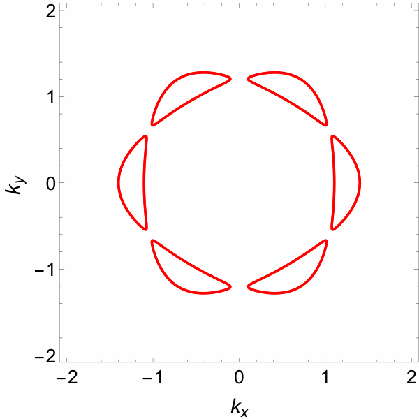
Diagonalizing the Hamiltonian gives the two normal state band dispersions, , each of which is two-fold degenerate. The Fermi surfaces are shown in Fig. 2 for the parameters from Ref. 35.
 |
|
|---|---|
II.2 Superconducting order parameter
The superconducting order parameter proposed in Ref. 35 is an state that can be written as . Here and are two basis functions of the representation, and , with overall pairing magnitude and a real number that controls the anisotropy of the order parameter. Due to the relative phase between and , is chiral, with the chirality determined by the sign of .
and are both triplets in spin as suggested by experiments [11, 40, 30]. The spatial parts of and contain not only - and -wave components but also a -wave component as discussed above. Spatial inversion operation not only transforms but also interchanges the two sublattices. The - and -wave components are odd functions of and triplets in the sublattice index, while the -component is an even function of but a sublattice singlet. As mentioned above, the pairing amplitudes of the - and -wave components connect different sublattices while the -wave component pairs sites on the same sublattice. The - and -components are of similar magnitude while the -wave is smaller. In the following, we will ignore this small -component. Then the two basis functions and can be written as [35]
| (7a) | ||||
| (7b) | ||||
where, for nearest-neighbor intersublattice pairing,
| (8a) | ||||
| (8b) | ||||
| (8c) | ||||
| (8d) | ||||
In the expressions for and , the spin Pauli matrix indicates that the spin triplet pairing vector is along the -direction (or the crystal -axis). The presence of sublattice Pauli matrices and comes from the fact that the - and -wave components are derived from the real and imaginary part, respectively, of a pairing amplitude for electrons from NN inter-sublattice ions. Because of the mixing between the - and -wave components,
| (9) |
has a term which is not proportional to the identity matrix , which makes nonunitary [41]. In Eq. (9),
| (10a) | ||||
| (10b) | ||||
II.3 Reduction of the BdG Hamiltonian
The expressions for and defined above can now be substitued into the BdG Hamiltonian given by Eq. (4). One finds reduces to two decoupled blocks:
| (11) |
with
| (12a) | |||
| (12b) | |||
The two bases are
| (13a) | |||
| (13b) | |||
In the above equations, , and , where are sublattice labels. The two blocks are connected to each other by spin inversion, , which leaves all matrix elements of and unchanged except for a change in the sign of the SOC term, . However, as will be shown later, the Hall conductivity is an even function of . Therefore we only need to focus on one block, say , and multiply the computed for that block by a factor of two. An additional factor of 1/2, arising from the double-counting of degrees of freedom in BdG theory, will cancel this factor of 2. Hereafter, we drop the superscript in and simply denote it as for brevity. Note that this decomposition into two blocks is only possible in the absence of the intralayer -wave pairing.
From one can obtain the Bogoliubov quasiparticle energies, which have line nodes on the plane that form six rings, as shown in Fig. 3. These nodal rings are counter examples to Blount’s theorem [42, 43, 44, 45, 46, 47] and are topologically protected as a joint consequence of both the non-symmorphic group symmetries and the nonzero spin orbital coupling, as discussed in Refs. 45, 46, 47.
III Computation of the anomalous Hall conductivity
The Hall conductivity can be computed from the Kubo formula [48, 19]
| (14) |
where is the electric current density - correlator. At the one-loop level is given by (setting )
| (15) |
where is the temperature (set to at the end of the calculation) and and are fermionic and bosonic Matsubara frequencies, respectively. is the Green’s function of the block Hamiltonian with inverse defined by
| (16) |
From one obtains the Bogoliubov quasiparticles energies of the Hamiltonian . However, the equation to be solved is not a quadratic equation for but a quartic equation in (see Eq. (40) in App. A). Consequently, the analytic expressions for the quasiparticle energies as well as the final expression for are quite lengthy, and these results are summarized in App. A in Eqs. (42) to (46b). From these expressions it is difficult to identify which ingredients are essential to obtain a nonzero , and so we also compute perturbatively to obtain a much simpler expression that is valid at intermediate to high frequencies.
We treat the -wave component of the superconducting order parameter as a perturbation and write where
| (17) |
and
| (18) |
and will be taken as the “unperturbed” and “perturbed” Hamiltonian, respectively. We choose this particular partition because it is precisely the component superconducting order parameter part that makes the Bogoliubov quasiparticle energy expression complicated (see Eq. (40) in App. A) and also because, as we will see later, the leading order contribution to is linear in .
Since we are including the effect of only perturbatively, the results are only reliable for sufficently large . Actually, the perturbative expansion is in , not just (see Eq. (40) in App. A for details). So, the perturbative results are reliable for , where is the SOC strength. The full Green’s function results and the perturbative results for , are compared in App. A in Figs. 7 and 8, showing the two are essential identical beyond . Since the laser frequency at which the Kerr effect has been measured is [5], which is in our model, the perturbative results can be used to compare to experiment.
III.1 Perturbative calculation
Here we discuss the perturbative calculation of , with further details given in App. B. Quantities of different order in are represented by superscripts . First, consider zeroth order described by the Hamiltonian . The Bogoliubov quasiparticle energies, , are
| (19) |
with
| (20a) | ||||
| (20b) | ||||
which are slightly different from those of the full Hamiltonian . However still has nodal rings on the plane that are almost identical to those obtained from the full Hamiltonian, , plotted in Fig. 3. These nodal rings are protected by the non-symmorphic space group symmetry and spin-orbit coupling [45, 35].
The velocity operators, which appear in Eq. (15), are defined by the normal state Hamiltonian, , which can be written in terms of the sublattice Pauli matrices, :
| (21) |
with and . Then [15, 19], where is the identity matrix for the Nambu space, or written out explicitly,
| (22) |
with and . can be obtained from by the substitution: . With and , one can compute the zeroth order current-current correlator from Eq. (15). However, a direct computation shows that , so that . In other words, a chiral -wave superconducting order parameter alone does not give rise to a non-zero anomalous Hall conductivity from the multiband mechanism if the two bands arise from stacking. The mixing between -wave and -wave components is crucial for a nonzero and one needs to go to first order to calculate a non-zero .
From the full Green’s function , one can define the first order Green’s function as and, from Eq. (15), the first order current-current correlator is
| (23) |
This (or, more precisely, ) is evaluated in App. B by first writing the velocity operators and Green’s functions as linear combinations of Pauli matrices to simplify computing the trace and then doing the Matsubara sum. After performing a Wick rotation, , one obtains the final expression for the Hall conductivity,
| (24) |
where for brevity we have suppressed the infinitesimal imaginary part, , in . is an anti-symmetrized velocity factor given by
| (25) |
We have also introduced two frequency dependent functions in Eq. (24), which are defined as (for details see App. B)
| (26) |
and
| (27) |
with and given by
| (28a) | ||||
| (28b) | ||||
| (28c) | ||||
The sign means only the leading order terms in and have been kept. There are seven frequency independent coefficients in the numerators of and . Their expressions are
| (29a) | ||||
| (29b) | ||||
| (29c) | ||||
| (29d) | ||||
| (29e) | ||||
The subscripts, , in these coefficients directly reflect the corresponding physical processes that they are associated with, which can be inferred from the denominator of each term in the expressions of , and . For example, the first term in with coefficient corresponds to a process where a Cooper pair, with momentum , is broken and a Bogoliubov quasiparticle pair with energies, and , are excited by the incident photon with a frequency . The two Bogoliubov quasiparticles have the same momentum as the broken Cooper pair because the incident photon momentum relative to . Energy conservation of this process requires , which explains the denominator in the first term in . Other terms in , and can be interpretated in a similar way. Notice that in the expressions for , and there is no term with a denominator , which would correspond to a process where a preexisting Bogoliubov quasiparticle with an energy gets excited to a higher energy level of by the incident photon.
Finally, as noted below Eq. (13b), we can see from Eqs. (26)-(27), that is an even function of , since the two functions and depend on only through , which are even in (see Eq. (19)); does not depend on (see Eq. (25)), and the factor is also even in because the mixed product contributes one and only one since .
Next we evaluate the expression for in Eq. (24) numerically. Replacing with in Eq. (24), the imaginary part can be written as
| (30) |
where and are:
| (31a) | ||||
| (31b) | ||||
The summation in Eq. (30) is calculated numerically for each and the results are plotted in Fig. 4 over two different ranges of so that the details at larger , where is smaller, can be clearly seen. has several sign changes as a function of because the different factors in Eq. (30) change sign at different positions with different quasiparticle energies. Also note that is non-zero for arbitrarily small since the external field can excite quasiparticle pairs at arbitrarily small energy near the line nodes in the superconducting gap. Although vanishes as , this feature is not visible in Fig. 4 (left panel) because the crossover to small behavior occurs at very small frequency, (see Fig.6 of Ref. 35).
The real part, , can be computed from the data for by the Kramers-Kronig transformation,
| (32) |
where stands for Cauchy principal value integral. The results for are plotted in Fig. 5. In the right panel of Fig. 5, the red dashed line is an exact high frequency asymptotic result, whose expression is given by [49]
| (33) |
where is an equal time commutator and the expectation value is with respect to the ground state of the BdG Hamiltonian. In App. C, we compute to first order in and find . Similar to , has further structure at very low frequency, . It saturates to a constant with a zero slope as . Again, due to the large frequency range in Fig. 5 (left panel), this feature is not visible.
III.2 Discussions of
From Eq. (24), we can identify the necessary ingredients for to be nonzero. As emphasized previously, both the chiral -wave and the chiral -wave components need to be present. In particular, the dependence of on these two parameters is through the combination , which is proportional to the chirality. Under time reversal, this combination, and consequently , changes sign. This can be seen explicitly from the fact that under time reversal, , and . This is the only combination quadratic in and/or that is odd under time-reversal. It is also this term that makes the order parameter nonunitary.
The second important ingredient for is the complex inter-sublattice hopping, , since both velocity terms appearing in Eq. (24), and , vanish if is real. These velocity terms are consistent with another general requirement for to be nonzero in the multi-band mechanism. Namely, some antisymmetrized products of the velocity operators, (where label orbitals or, in our case, sublattices) need to be nonzero. Note that SOC, , is not necessary for a nonzero . Of the two terms in Eq. (24), only the first term vanishes if . The second term, with , only depends on through the Bogoliubov quasiparticle energies and remains nonzero if the SOC is absent.
The two key ingredients identified above, the mixing of the chiral - and -wave order parameters and the complex inter-sublattice hopping, , are both direct consequences of the non-symmorphic symmetry of . They would both be absent if the lattice were symmorphic. In this sense, the terms that we have identified for are unique to non-symmorphic chiral superconductors.
The two terms in Eq. (24) can be represented by Feynman diagrams, which are shown in Fig. 6. For each diagram in Fig. 6, the time-reversed diagram needs to be subtracted.
There are two types of diagrams. In Fig. 6(a) only one of the two vertices involves two different orbitals; while in Fig. 6(b) both the vertices involve transitions between different orbitals. Of the two terms in Eq. (24), the term only contributes to Fig. 6(b), while the other term, , is a mixture of Fig. 6(a) and 6(b). This is because can be written as a sum of and , of which the former and latter correspond to Fig. 6(a) and Fig. 6(b), respectively. In the band basis, the term in Eq. (24) corresponds to Fig. 6(a) (with now labelling bands), rather than Fig. 6(b) as in the orbital basis; while the whole term corresponds to Fig. 6(b). It is clear in the band basis that both Fig. 6(a) and Fig. 6(b) vanish if the inter-band pairing is zero, similar to what was found in Ref. 19.
Note that Fig. 6(b) type of diagram is absent in Ref. 19 because the model studied there has a real inter-orbital hopping , which makes the contribution from Fig. 6(b) with the photon polarization exactly cancel the same diagram with . On the other hand, Fig. 6(a) vanishes in the current model unless is complex, while it survives in Ref. 19 for real inter-orbital hopping, due to the different way the inter-orbital pairing arises in the two models.
also needs to obey the following two sum rules [50, 51],
| (34) | ||||
| (35) |
where Eq. (35) is analogous to the well-known optical conductivity -sum rule. In App. C, we show these sum rules are satisfied, both analytically and numerically, by .
Lastly we mention that the Hall conductivity, quite generally, needs to satisfy several symmetry constraints. Under time reversal, all vertical mirror reflections, and particle-hole interchange, must reverse its sign. Both given in Eq. (24), and the full Green’s function result of given in App. A are consistent with these symmetry constraints.
IV Estimation of the Kerr rotation angle
From the numerical results of , the Kerr rotation angle, , can be estimated using Eq. (1), which also involves the complex index of refraction, . Here we use our results to estimate the Kerr angle for , where was measured [5] at a laser frequency .
We first estimate = from experimental data. By definition , where is related to the conductivity, , by and is the high frequency limit dielectric constant. We extract = from the experimental data of Ref. 52. Taking , we obtain =, which gives an index of refraction,
| (36) |
To obtain a value for , we need to estimate the in-plane hopping parameter in eV, since we have scaled all energies by . This can be obtained by comparing the normal state band dispersions of our two-band model along the symmetry directions in the plane to the corresponding first-principle calculation results from Ref. 53. The comparison gives (for details, see App. D). This value of corresponds to at . From our numerical results for in Fig. 4 and Fig. 5 we obtain, at ,
| (37) |
where is the -axis lattice spacing of . From Eqs. (36), (37) and (1), the Kerr angle is then,
| (38) |
Our estimated is about an order of magnitude smaller than the experimental value of about 350 nanoradians measured at the lowest temperatures [5]. However, it may still be a significant contribution to the explanation for the Kerr measurement on [5] given that there are uncertainties in the optical constants, the band parameters, and the magnitude of used for this estimate. We briefly comment on these uncertainties.
Ideally, one would like measurements of on the same crystal used for the Kerr measurements. Other optical data on would give somewhat different results [54, 55, 56], although we estimate that the uncertainty in the optical data is unlikely to change the estimated Kerr angle by more than a factor of 3 or so.
As to the band parameters, uncertainty comes both from the value of and from the fact that a very simplified nearest-neighbour hopping model has been used to approximate the two bands which give rise to the starfish Fermi surface. This likely introduces a larger uncertainty than that from errors in the estimate of .
The other parameter that can greatly affect the size of is , the amplitude of the gap function written in the orbital basis. Note that is not the gap that one would observe in tunneling measurements. Defining as the position of the coherence peak in the Bogoliubov quasiparticle density of states spectrum, one finds (see Fig.6 of Ref. 35). Experiments have found values for of 0.04 meV [57], 0.1 meV [58], and more recently, 0.5 meV [31]. The parameters we used, taken from Yanase [35], with meV, corresponds to meV, roughly consistent with the most recent experimental value. Since the Kerr angle scales quadratically with the gap magnitude, smaller values of would give much smaller values of . For example, setting K, we find meV for our model in the weak-coupling limit, which would reduce by a factor of 26.
Lastly there are several other Fermi surface sheets that we did not take into account, which might contribute to . These additional contributions could either increase or decrease the total , depending on their relative magnitude and sign.
With these uncertainties in mind, we conclude that the that we have identified here can be significant for explaining the Kerr measurement on , even if it is not large enough to account for the whole experimentally observed signal. Further experiments and theoretical studies are needed to resolve the above uncertainties.
V Conclusion and Discussions
To summarize, by considering a simplified two band model that results from ABAB stacking for the starfish-like Fermi surface of , we have identified a contribution to the ac anomalous Hall conductivity for within the intrinsic multiband chiral superconductivity mechanism. The Kerr angle estimated from the computed Hall conductivity can be significant for understanding the Kerr measurement on . This mechanism requires non-zero interband pairing. Since intra- and inter-band pairing are indistinguishable at the six points on the plane where the starfish-like Fermi surfaces of UPt3 intersect, this is a useful model for studying the multiband chiral superconductivity mechanism.
We have identified two crucial ingredients for the nonzero : a complex inter-sublattice hopping between sites and a novel superconducting order parameter that involves mixing between chiral -wave and chiral -wave pairing. Both of these are consequences of the nonsymmorphic group symmetry of the crystal lattice. If the inter-sublattice hopping is real or if one of the chiral - and -wave pairing components is absent, then and vanish. This is a generalization of, albeit somewhat distinct from, the multiband chiral superconductivity mechanism for the anomalous ac Hall effect in a chiral -wave superconductor [19]. The and contribution that we have discussed here can also be applied to other nonsymmorphic chiral superconductors.
In our analysis we have identified two types of terms that contribute to at each point, as can be seen from Eq. (24). One term does not require SOC, while the other does. The two make comparable contributions to . However, these two contributions in general can have different signs at different points, which results in multiple sign changes of as a function of . Because of these sign changes the estimated Kerr angle can be sensitive to the band parameters as well as to the laser frequency used in the Kerr measurement. Therefore future Kerr measurements at different frequencies would be very helpful in determining how relevant the Kerr angle contribution identified here is to .
We should mention that in our calculation we have neglected a small chiral -wave component pairing in the original proposed superconducting order parameter of Ref. 35. This component is also symmetry allowed but is expected to be energetically less favorable compared with the dominant chiral - and -components. In the two band model we consider, this -wave component alone can also give rise to a nonzero . This contribution relies on the nonunitary nature of the -wave pairing (it pairs only one spin component if ), and requires nonzero SOC and complex inter-sublattice hopping. Presumably the admixture of this neglected small -wave component will not significantly alter the estimated Kerr angle simply because its pairing amplitude is thought to be very small..
Recently the authors of Ref. 59 suggested that the Kerr rotation in can not be understood without invoking pairing in completely filled or empty bands because the laser frequency used in the Kerr angle measurement [5], , is bigger than the normal state bandwidth of the partially filled bands of . However, this does not need to be the case for two reasons. First, since the incident photon breaks a Cooper pair and generates two Bogoliubov quasiparticles, the maximum energy cost is not the bandwidth, but twice the energy difference between the Fermi level and the bottom or top of the band (whichever is greater). From Ref. 60, this maximum energy along the symmetry direction in the plane is about , while from Ref. 53, this is about . The latter (which we used to determine the hopping in our model) allows energy-conserving transitions within the band at 0.8 eV. Second, both and can make significant contributions to . Even if the laser frequency is larger than the excitation energy of two quasiparticles within the band, will still be nonzero at . Consequently, the observation of nonzero in at 0.8 eV may still be understood within a model of partially filled bands.
VI Acknowledgements
We would like to thank Tom Timusk and Steve Kivelson for helpful discussions. This work is supported in part by NSERC (CK and ZW), the Canada Research Chair program (CK), the National Science Foundation under Grant No. NSF PHY11-25915 (AJB, CK, GZ), the Gordon and Betty Moore Foundation’s EPiQS Initiative through Grant GBMF4302 (AJB and CK), the ANR-DFG grant Fermi-NESt (GZ), and a grant from the Simons Foundation (395604 to CK). AJB, CK and GZ greatly appreciate the hospitality provided by the Kavli Institute for Theoretical Physics at UCSB and (for AJB, CK and ZW) the hospitality of the Stanford Institute for Theoretical Physics, where part of the work was completed.
Appendix A Full Green’s function calculation of
As mentioned in the main text, the full Green’s function calculation is much more involved than the perturbative calculation. Here, we present some main steps for the full calculation of , omitting detail of derivations.
We first establish some notation. We denote the four Bogoliubov quasiparticle energies of the BdG Hamiltonian , from Eq. (12a) of the main text, as , with . The are solutions to
| (39) |
which can be expanded as
| (40) |
where the three coefficients are given by
| (41a) | ||||
| (41b) | ||||
| (41c) | ||||
Eq. (40) is a quartic equation for rather than a quadratic equation in due to the term. Because of this, the solutions do not occur as particle hole pairs. However, this does not contradict the particle-hole symmetry of the full superconducting BdG Hamiltonian which is restored when is combined with the other block , given in Eq. (12b), to form the full . Also, because of the term in Eq. (40), the expressions for the , in terms of the three coefficients are much more complicated than in the case of . For brevity we will not present them here.
With the coefficients and defined above we can now write the final result for as follows
| (42) |
where was defined in Eq. (25). In Eq. (42) the three frequency dependent functions are defined as
| (43a) | ||||
| (43b) | ||||
| (43c) | ||||
and are connected to the three functions, , that we introduced in our perturbative calculations, by
| (44) |
where are the two Bogoliubov quasiparticle energies of the zeroth order Hamiltonian(see Eq. (19)). From these relations we see that the parameter that controls our perturbative calculation is rather than simply .
The term in Eq. (42) contains terms of higher powers, fourth order in and , compared with the other terms that are second order in and (ignoring the dependence through the quasiparticle energies ). This is clear from Eq. (41b), the expression for , and from
| (45) |
where we have introduced two additional anti-symmetrized velocity products and , defined as follows
| (46a) | ||||
| (46b) | ||||
From in Eq. (42) we can derive its imaginary part, . Then we can numerically evaluate and compare the results with our perturbation results for in the main text. The comparison is given in Fig. 7. We see that the two are quite different for , but they are essentially indistinguishable for .
We can also compute by the Kramers-Kronig transformation and compare the results with , presented in the main text. This comparison is shown in Fig. 8. Again at the two agree well.
Appendix B Derivation of
In order to compute , using Eq. (14) and (23), we introduce the function such that
| (47) |
From the expression for in Eq. (23), we can write as follows
| (48) |
This expression contains traces of products of matrices and . To complete these traces we decompose the matrices into linear combinations of , where and are Pauli matrices for the sublattice and particle-hole Nambu subspaces, respectively. Then
| (49) | ||||
| (50) |
We choose the following basis for the above decomposition
| (51) | ||||
| (52) |
where and . In Eq. (50), and elsewhere, summations over repeated indices are assumed. In order to extract the coefficients and it will be convenient to introduce both the conjugate of , denoted as , and also the conjugate of , denoted as . Their definitions are
| (53) |
Different components of the vectors and satisfy an orthonormal relation: . Using this relation we can obtain the coefficients in Eq. (50) as follows,
| (54) | ||||
| (55) |
Substituting Eq. (50) into the expression for in Eq. (48) gives
| (56) |
where we have suppressed the arguments of the Green’s functions. However, it should be kept in mind that in each of the two-Green’s function products, the first Green’s function should be evaluated at ; while the second should be evaluated at . The trace over Pauli matrix products in Eq. (56) is trivial: . The other trace, , is nonzero only for two cases: all four indices, , are different from each other; the four indices consist of two identical pairs. However, the latter contribution is even with respect to the interchange and therefore contributes zero to after the antisymmetrization, . Therefore the only non-zero contribution comes from the case with all four indices different. Because each of the indices,, can take four possible values there are different terms in total. However, half of them are zero because of the following three identities
| (57a) | ||||
| (57b) | ||||
| (57c) | ||||
Then we are left with
| (58) |
In obtaining this equation we have used the trace identity as well as its permutations.
Next we need to complete the the Matsubara summation in Eq. (47). This can be done for each of the three lines in Eq. (58). The derivations are quite lengthy, and we do not present them here. The final results are:
| (59a) | ||||
| (59b) | ||||
| (59c) | ||||
For brevity we have introduced two frequency dependent functions, and , which are defined as
| (60) | ||||
| (61) |
where the sign means only terms of leading order in and have been kept. and are given by
| (62a) | ||||
| (62b) | ||||
where , , , , , , , and are eight independent coefficients. The expressions for , , , , , and were given in Eqs. (29a)-(29e). The other two coefficients are as follows
| (63) |
Notice that both the term in Eq. (62a) and the term in Eq. (62b) have a second order pole at on the complex plane; while all other terms have first order poles. The second order poles appear only in the perturbative calculation but not in the full calculation. Numerically we found that the second order pole contributions to from Eq. (62a) and (62b) are negligible at , where is the SOC coupling strength. Hence we will ignore them hereafter. Performing a Wick rotation, , we see that and are given by Eqs. (26) and (27).
Now inserting the results from Eqs. (59a)-(59c) into the expression for in Eq. (58) we obtain
| (64) |
where we have used
| (65) |
and also introduced a notation for the following anti-symmetrized velocity factor
| (66) |
With these compact notations one can substitute from Eq. (64) back into Eq. (47) and obtain the final expression for the Hall conductivity as a function of frequency given in Eq. (24).
Appendix C Asymptotic result for large and sum rules
In this section we compute on the right hand side of Eq. (33) for the BdG Hamiltonian in Eq. (12a) up to first order in . Denote the basis of the Hamiltonian from Eq. (12a) as . Then the current operator can be written as , with . The velocity operator matrix is given in Eq. (22). Using the fact that the equal time expectation value , we obtain
| (67) |
with and given by
| (68a) | ||||
| (68b) | ||||
On the right hand side of Eq. (67) all Green’s function matix elements are evaluated at .
In Eq. (67) if we use the zeroth order result, , for all the Green’s function matrix elements then we obtain . This is consistent with Eq. (33) and the fact that .
The nonzero comes from the next order contribution: . Substituting the matrix elements of the first order Green’s function, , into Eq. (67) and completing the Matsubara summation,
| (69) |
where is defined in Eq. (25). The remaining summation in Eq. (69) can be evaluated numerically and the final result is . Then Eq. (33) becomes
| (70) |
It is also possible to perform the integral in Eq. (35) analytically using from Eq. (30). The result is identical to times Eq. (69). Similarly the integral of Eq. (34) can be performed analytically using Eq. (24)-(28c). The zero result follows from the analytic structure of the in Eq. (28a)-(28c). We also numerically evaluate the two sides of Eq. (34) and (35) using the data from Figs. 4 and 5 and confirm that Eqs. (34) and (35) are well satisfied.
Appendix D Estimation of the NN hopping
We plot the two normal state energy band dispersions along high symmetry directions in Fig. 9.
From the dispersions along , the corresponding band width in the plane is . We can fit this to the first-principles calculation results from Ref. 53. From the Supplemental Material Fig.S1(b), we estimate that the bandwidth of the dispersions along is . Therefore, as an estimation, .
We note that the bands along in Fig. 9 are far below the Fermi energy, which is inconsistent with the realistic first principle calculation result in Ref. 53. This is due to the oversimplification of our model which consists of only two bands resulting from the stacking. Due to this oversimplification, the dispersions along are not realistic. In order to estimate how these unrealistic dispersions affect our calculations of , we have recomputed by excluding all points that satisfy , where is the band bottom of the dispersions along in Fig. 9. The result is similar to the value obatined in the main text without this truncation. In other words, the unrealistic dispersions along do not significantly change our conclusion for . This is because the main contribution to comes from values closer to and not from the region near in the BZ.
References
- [1] C. Kallin and J. Berlinsky, Reports on Progress in Physics 79, 054502 (2016).
- [2] A. Kapitulnik, J. Xia, E. Schemm, and A. Palevski, New Journal of Physics 11, 055060 (2009).
- [3] P. N. Argyres, Phys. Rev. 97, 334 (1955).
- [4] J. Xia, Y. Maeno, P. T. Beyersdorf, M. M. Fejer, and A. Kapitulnik, Phys. Rev. Lett. 97, 167002 (2006).
- [5] E. R. Schemm, W. J. Gannon, C. M. Wishne, W. P. Halperin, and A. Kapitulnik, Science 345, 190 (2014).
- [6] E. R. Schemm, R. E. Baumbach, P. H. Tobash, F. Ronning, E. D. Bauer, and A. Kapitulnik, Phys. Rev. B 91, 140506 (2015).
- [7] E. Levenson-Falk, E. Schemm, M. Maple, and A. Kapitulnik, arXiv preprint arXiv:1609.07535 (2016).
- [8] X. Gong, M. Kargarian, A. Stern, D. Yue, H. Zhou, X. Jin, V. M. Galitski, V. M. Yakovenko, and J. Xia, Science Advances 3, e1602579 (2017).
- [9] C. Kallin and A. J. Berlinsky, Journal of Physics: Condensed Matter 21, 164210 (2009).
- [10] A. P. Mackenzie, T. Scaffidi, C. W. Hicks, and Y. Maeno, Quantum Materials 2, 40 (2017).
- [11] J. Sauls, Advances in Physics 43, 113 (1994).
- [12] M. Norman, Physica C: Superconductivity 194, 203 (1992).
- [13] N. Read and D. Green, Phys. Rev. B 61, 10267 (2000).
- [14] R. Roy and C. Kallin, Phys. Rev. B 77, 174513 (2008).
- [15] R. M. Lutchyn, P. Nagornykh, and V. M. Yakovenko, Phys. Rev. B 80, 104508 (2009).
- [16] J. Goryo, Phys. Rev. B 78, 060501 (2008).
- [17] E. J. König and A. Levchenko, Phys. Rev. Lett. 118, 027001 (2017).
- [18] S. K. Yip and J. A. Sauls, Journal of Low Temperature Physics 86, 257 (1992).
- [19] E. Taylor and C. Kallin, Phys. Rev. Lett. 108, 157001 (2012).
- [20] E. Taylor and C. Kallin, Journal of Physics: Conference Series 449, 012036 (2013).
- [21] K. I. Wysokiński, J. F. Annett, and B. L. Györffy, Phys. Rev. Lett. 108, 077004 (2012).
- [22] M. Gradhand, K. I. Wysokinski, J. F. Annett, and B. L. Györffy, Phys. Rev. B 88, 094504 (2013).
- [23] V. P. Mineev, Phys. Rev. B 89, 134519 (2014).
- [24] W. Huang, S. Lederer, E. Taylor, and C. Kallin, Phys. Rev. B 91, 094507 (2015).
- [25] Y. Tada, W. Nie, and M. Oshikawa, Phys. Rev. Lett. 114, 195301 (2015).
- [26] G. E. Volovik, JETP Letters 100, 742 (2015).
- [27] R. A. Fisher, S. Kim, B. F. Woodfield, N. E. Phillips, L. Taillefer, K. Hasselbach, J. Flouquet, A. L. Giorgi, and J. L. Smith, Phys. Rev. Lett. 62, 1411 (1989).
- [28] G. Bruls, D. Weber, B. Wolf, P. Thalmeier, B. Lüthi, A. d. Visser, and A. Menovsky, Phys. Rev. Lett. 65, 2294 (1990).
- [29] S. Adenwalla, S. W. Lin, Q. Z. Ran, Z. Zhao, J. B. Ketterson, J. A. Sauls, L. Taillefer, D. G. Hinks, M. Levy, and B. K. Sarma, Phys. Rev. Lett. 65, 2298 (1990).
- [30] R. Joynt and L. Taillefer, Rev. Mod. Phys. 74, 235 (2002).
- [31] J. Gouchi, A. Sumiyama, A. Yamaguchi, G. Motoyama, N. Kimura, E. Yamamoto, Y. Haga, and Y. Ōnuki, Journal of Physics: Conference Series 592, 012066 (2015).
- [32] S. M. Hayden, L. Taillefer, C. Vettier, and J. Flouquet, Phys. Rev. B 46, 8675 (1992).
- [33] B. Lussier, B. Ellman, and L. Taillefer, Phys. Rev. B 53, 5145 (1996).
- [34] The splitting of these two transitions has been attributed to very weak antiferromagnetic order (which we ignore in our analysis). See, for example, J.A. Sauls, Adv. Phys. 43, 113 (1994).
- [35] Y. Yanase, Phys. Rev. B 94, 174502 (2016).
- [36] Note that the crystal strcuture of is far from the ideal hcp structure. atoms in each layer form a hexagonal lattice with a atom between each nearest-neighbor pair of atoms, which means that the lattice of atoms in each layer is greatly expanded compared, for example to Uranium metal. By comparison, the nearest-neighbor distance for neighboring layers is much shorter, only of the intralayer distance. The axis distance is also rather short, wth ratio of only , compared to the ideal hcp ratio of .
- [37] G. J. McMullan, P. M. C. Rourke, M. R. Norman, A. D. Huxley, N. Doiron-Leyraud, J. Flouquet, G. G. Lonzarich, A. McCollam, and S. R. Julian, New Journal of Physics 10, 053029 (2008).
- [38] M. H. Fischer, F. Loder, and M. Sigrist, Phys. Rev. B 84, 184533 (2011).
- [39] D. Maruyama, M. Sigrist, and Y. Yanase, Journal of the Physical Society of Japan 81, 034702 (2012).
- [40] H. Tou, Y. Kitaoka, K. Ishida, K. Asayama, N. Kimura, Y. Onuki, E. Yamamoto, Y. Haga, and K. Maezawa, Phys. Rev. Lett. 80, 3129 (1998).
- [41] M. Sigrist and K. Ueda, Rev. Mod. Phys. 63, 239 (1991).
- [42] E. I. Blount, Phys. Rev. B 32, 2935 (1985).
- [43] M. R. Norman, Phys. Rev. B 52, 15093 (1995).
- [44] T. Micklitz and M. R. Norman, Phys. Rev. B 80, 100506 (2009).
- [45] S. Kobayashi, Y. Yanase, and M. Sato, Phys. Rev. B 94, 134512 (2016).
- [46] T. Micklitz and M. R. Norman, Phys. Rev. B 95, 024508 (2017a).
- [47] T. Micklitz and M. R. Norman, Phys. Rev. Lett. 118, 207001 (2017b).
- [48] G. D. Mahan, Many-Particle Physics (Plenum Press, 1990).
- [49] B. S. Shastry, B. I. Shraiman, and R. R. P. Singh, Phys. Rev. Lett. 70, 2004 (1993).
- [50] E. Lange and G. Kotliar, Phys. Rev. Lett. 82, 1317 (1999).
- [51] H. D. Drew and P. Coleman, Phys. Rev. Lett. 78, 1572 (1997).
- [52] P. E. Sulewski, A. J. Sievers, M. B. Maple, M. S. Torikachvili, J. L. Smith, and Z. Fisk, Phys. Rev. B 38, 5338 (1988).
- [53] T. Nomoto and H. Ikeda, Phys. Rev. Lett. 117, 217002 (2016).
- [54] J. Schoenes and J. Franse, Physica B+C 130, 69 (1985).
- [55] M. Dressel, N. Kasper, K. Petukhov, B. Gorshunov, G. Grüner, M. Huth, and H. Adrian, Phys. Rev. Lett. 88, 186404 (2002).
- [56] F. Marabelli, G. Travaglini, P. Wachter, and J. Franse, Solid State Communications 59, 381 (1986).
- [57] G. Goll, H. v. Löhneysen, I. K. Yanson, and L. Taillefer, Phys. Rev. Lett. 70, 2008 (1993).
- [58] G. Goll, C. Bruder, and H. v. Löhneysen, Phys. Rev. B 52, 6801 (1995).
- [59] R. Joynt and W.-C. Wu, Scientific Reports 7, 12968 (2017).
- [60] C. S. Wang, M. R. Norman, R. C. Albers, A. M. Boring, W. E. Pickett, H. Krakauer, and N. E. Christensen, Phys. Rev. B 35, 7260 (1987).