On the Distribution, Model Selection Properties and Uniqueness of the Lasso Estimator in Low and High Dimensions

The distribution of the Lasso estimator (Tibshirani, 1996) has been an object of study in the statistics literature for a number of years. The often cited paper by Knight & Fu (2000) gives the asymptotic distribution of the Lasso in the framework of conservative model selection in a low-dimensional (fixed-$p$) framework by listing the limit of the corresponding stochastic optimization. Pötscher & Leeb (2009) derive explicit expressions of the distribution in finite samples as well as asymptotically for all large-sample regimes of the tuning parameter (“conservative” as well as “consistent model selection”) in the framework of orthogonal regressors. More recently, Zhou (2014) gives high-level information on the finite-sample distribution for arbitrary designs in low and high dimensions, geared towards setting up a Monte-Carlo approach to infer about the distribution. In Ewald & Schneider (2018), the large-sample distribution of the Lasso is derived in a low-dimensional framework for the large-sample regime of the tuning parameter not considered in Knight & Fu (2000). Moreover, Jagannath & Upadhye (2018) consider the characteristic function of the Lasso to obtain approximate expressions for the marginal distribution of one-dimensional components of the Lasso when these components are “large”, therefore not having to consider the atomic part of the estimator.

In this paper, we exactly and completely characterize the distribution of the Lasso estimator in finite samples in the context of a linear regression model with normal errors. In low dimensions, we give formulae for the cumulative distribution function (cdf), as well as the density functions conditional on which components of the estimator are non-zero. We do so assuming full column rank of the regressor matrix. Our results do not hinge on the normality assumption of the errors, but can easily be extended to more general error distributions. We also exactly quantify the correspondence between the Lasso and least-squares (LS) estimator, depending on the regressor matrix and tuning parameters only.

In a high-dimensional setting, we make absolutely no assumptions on the regressor matrix. We give formulae for the probability of the Lasso estimator falling into a given set and exactly quantify the relationship between the Lasso estimator and the data object $X^{\prime}y$. Through this relationship, we also learn that the Lasso may never select certain models, this property depending only on the regressor matrix and the penalization weights and being independent of the observed response vector. In fact, we can characterize a so-called structural set that contains all covariates that are part of a Lasso model model for some response vector. This structural set can be identified by how the row space of the regressor matrix intersects a cube centered at the origin whose side lengths are determined by the penalization weights. The set may not contain all indices, in which case the Lasso estimator will rule out certain covariates for all possible observations of the dependent variable. This is related to the idea of so-called SAFE rules (Tibshirani et al., 2012) that can discard covariates for Lasso solutions for a fixed value of the dependent variable.

Finally, we present a condition for uniqueness of the Lasso estimator that is both necessary and sufficient, again related to how the row space of the regressor matrix intersects the above mentioned cube. Previously, only a sufficient condition for uniqueness has been known (Tibshirani, 2013, Ali & Tibshirani, 2019, see e.g.). The results quantifying the relationship between the Lasso and the LS estimator or $X^{\prime}y$, respectively, are in fact completely independent of the error distribution and merely utilize the given values of the dependent variable and the regressor matrix. The results on model selection properties and uniqueness use the regressor matrix and penalization weights only.

The paper is organized as follows. We introduce the setting and notation in Section 2 and state basic results used throughout the paper. The low-dimension case is treated in Section 3, whereas we consider the high-dimensional case in Section 4. We conclude in Section 5.

Consider the linear model

where $y$ is the observed $n\times 1$ data vector, X is the $n\times p$ regressor matrix which is assumed to be non-stochastic, $\beta\in\mathbb{R}^{p}$ is the true parameter vector and $\varepsilon$ the unobserved error term. We assume that $X^{\prime}\varepsilon$ follows a $N(0,\sigma^{2}X^{\prime}X)$-distribution with $\sigma^{2}>0$, which, for instance, is the case when the components of $\varepsilon$ are independent and identically distributed according to a $N(0,\sigma^{2})$-distribution. Our results depend on the distribution of $X^{\prime}\varepsilon$ only, and we chose the normal distribution for presentation purposes.¹¹ 1 In fact, some of the following results are completely independent of the error distribution. These are Lemma 1 and Corollary 2, Theorems 8 and 12, Corollary 13 as well as Theorems 14 and 15.

We consider the weighted Lasso estimator $\hat{\beta}_{\textnormal{\tiny L}}$, defined as a solution to the minimization problem

where $\lambda_{n,j}$, are non-negative user-specified tuning parameters that will typically depend on $n$. To ease notation, we shall suppress this dependence for the most part and write $\lambda_{n,j}=\lambda_{j}$ for each $j$. Note that if $\lambda_{j}=0$ for all $j$, the weighted Lasso is equal to LS estimation, and that $\lambda_{1}=\dots=\lambda_{p}>0$ corresponds to the classical Lasso estimator as proposed by Tibshirani (1996), to which case we also refer to by uniform tuning. For later use, let $\lambda=(\lambda_{1},\dots,\lambda_{p})^{\prime}$ and define $\mathcal{M}_{0}=\{j:\lambda_{j}=0\}$, the index set of all unpenalized coefficients. If $\mathcal{M}_{0}\neq\varnothing$, we speak of partial tuning. Note that $\mathcal{M}_{0}$ contains the indices of covariates that will be part of any model chosen by the Lasso. We stress dependence on the unknown parameter $\beta$ when it occurs, but do not specify dependence on $X$, $y$ or $\lambda$ as these quantities are available to the user.

The following notation will be used throughout the paper. Let $\phi_{(\mu,\Sigma)}$ denote the Lebesgue-density of a normally distributed random variable with mean $\mu$ and covariance matrix $\Sigma$, and let $\Phi$ be the cdf of a univariate standard normal distribution. For a vector $m\in\mathbb{R}^{p}$ and an index set $I\subseteq\{1,\dots,p\}$, the vector $m_{I}\in\mathbb{R}^{|I|}$ contains only the components of $m$ corresponding to the elements of $I$. We write $|I|$ for the cardinality of $I$, and $I^{c}$ for $\{1,\dots,p\}\setminus I$, the complement of $I$. The $1$-norm of $m$ is denoted by $\|m\|_{1}$ whereas the $2$-norm is simply denoted by $\|m\|$. For $x\in\mathbb{R}$, let $\operatorname{sgn}(x)=\mathds{1}_{\{x>0\}}-\mathds{1}_{\{x<0\}}$ where $\mathds{1}$ is the indicator function. For a set $A\subseteq\mathbb{R}^{p}$, the set $m+A=A+m$ is defined as $\{m+z:z\in A\}$, with a analogous definitions for $A-m$ and $m-A$. We denote the Cartesian product by $\prod$ and the kernel, column space, and rank of a matrix $C$ by $\ker(X)$, $\operatorname{col}(C)$, and $\operatorname{rk}(C)$, respectively. The columns of $C$ are denoted by $C_{j}$ whereas $C_{I}$, for some index set $I$, is the matrix containing the $|I|$ columns of $C$ corresponding to indices in $I$ only. For a quadratic matrix $C$, $|C|$ denotes the determinant of $C$. We use $\mathbb{R}_{>0}$ for the positive, and $\mathbb{R}_{\geq 0}$ for the non-negative real numbers.

Let $\{D_{-},D_{0},D_{+}\}$ be a partition of $\{1,\dots,p\}$ into three sets, some of which may be empty. It will be convenient to also describe this partition by a vector $d\in\{-1,0,1\}^{p}$ with $d_{j}=\mathds{1}_{\{j\in D_{+}\}}-\mathds{1}_{\{j\in D_{-}\}}$. For such $d$, we denote by $\mathcal{O}^{d}=\{z\in\mathbb{R}^{p}:\operatorname{sgn}(z_{j})=d_{j}\text{ for }j=1,\dots,p\}=\{z\in\mathbb{R}^{p}:z_{j}<0\text{ for }j\in D_{-},z_{j}=0\text{ for }j\in D_{0},z_{j}>0\text{ for }j\in D_{+}\}$. Note that $m+\beta\in\mathcal{O}^{d}$ is short-hand notation for $m_{j}<-\beta_{j}$ for $j\in D_{-}$, $m_{j}=-\beta_{j}$ for $j\in D_{0}$ and $m_{j}>-\beta_{j}$ for $j\in D_{+}$. We write $D_{\pm}$ for $D_{-}\cup D_{+}$.

Finally, we state the conditions that characterize solutions to (2), known as the Kuhn-Karush-Tucker (KKT) conditions for the Lasso (see e.g. Tibshirani, 2013, with the slight adaptation that we use componentwise tuning) which form the basis of most proofs and will be used throughout the article.

Plugging in $y=X\beta+u$, we rewrite this as

Throughout this section, we assume that $X$ has full column rank $p$, implying that we are considering the low-dimensional setting where $p\leq n$. This assumption is used in the following through the fact that $W=X^{\prime}\varepsilon$ follows a non-degenerate normal distribution on $\mathbb{R}^{p}$ in the distributional statements on $\hat{\beta}_{\textnormal{\tiny L}}$ (Theorem 3, Corollary 5). It is additionally used through the fact that the true parameter is properly identified in the distributional statements concerning the estimation error $\hat{\beta}_{\textnormal{\tiny L}}-\beta$ (Corollary 4, Proposition 6, Theorem 7). We also rely on this assumption in Theorem 8 through the invertibility of $X^{\prime}X$ and the existence of the LS estimator.

Theorem 3 gives the distribution of $\hat{\beta}_{\textnormal{\tiny L}}$. The dependence on the unknown parameter $\beta$ arises in the shift $(m_{\beta})_{D_{0}}=-\beta_{D_{0}}$ as well as in the limits for the variables of integration $m_{D_{+}}$ and $m_{D_{-}}$. In case the regressors are orthogonal, more concretely, if $X^{\prime}X=I_{p}$, the probability expression in Theorem 3 can be written as

where $Z_{j}\overset{\text{\tiny{iid}}}{\sim}N(0,\sigma^{2})$, which is consistent with the well-known fact that the Lasso is equivalent to componentwise soft-thresholding in this case, also treated in Pötscher & Schneider (2009).

The distribution of the estimation error $\hat{u}=\hat{\beta}_{\textnormal{\tiny L}}-\beta$ can now be derived from Theorem 3 as a corollary.

Another direct consequence of Theorem 3 is a concrete formula for the probability of the extreme event of the Lasso setting all components equal to zero.

Theorem 3 now puts us into a position to fully specify the distribution of the Lasso estimator. In case $\lambda_{j}>0$ for all $j$, one easily sees from the preceding corollary that this distribution is not absolutely continuous with respect to the $p$-dimensional Lebesgue-measure, and thus no density exists. One can, however, represent the distribution through Lebesgue-densities after conditioning on which components of the estimator are negative, equal to zero, and positive, which we shall do in the sequel.

Besides the conditional densities, we can also specify the full cdf of $\hat{u}=\hat{\beta}_{\textnormal{\tiny L}}-\beta$ which is done in the following theorem.

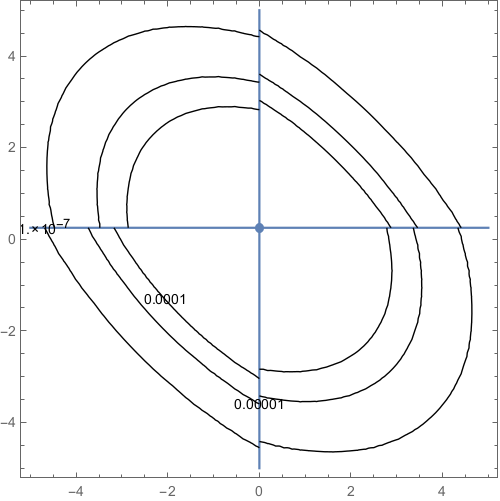
For illustration of Proposition 6 and Theorem 7, consider Figures 2 and 3 which display an example of the distribution of $\hat{u}=\hat{\beta}_{\textnormal{\tiny L}}-\beta$. One can see that the Lasso estimation error follows a shifted normal distribution, conditional on the event $\hat{u}_{j}\neq-\beta_{j}$ ($\hat{\beta}_{\textnormal{\tiny L},j}\neq 0$) for each $j$, with the shift depending on the signs of $\hat{\beta}_{\textnormal{\tiny L}}$, as can be seen in Figure 2. Figure 3 displays the mass which lies on the set $\{z\in\mathbb{R}^{2}:z_{1}=-\beta_{1},z_{2}\neq 0\}$, that is, the density functions $h^{(0,1)}$ and $h^{(0,-1)}$ on their corresponding domains. The mass on the set $\{z\in\mathbb{R}^{2}:z_{1}\neq 0,z_{2}=-\beta_{2}\}$ looks qualitatively similar to Figure 3. Note that we also have point-mass at $-\beta$, as is pointed out by Corollary 5.

We now turn to the main case of this this article, the high-dimensional setting where $p>n$. We make no assumptions on the regressor matrix $X$ in this section. Using similar arguments as in the case $p\leq n$, we can again start by characterizing the distribution of the Lasso, albeit in a somewhat less explicit form. Note that we have $\operatorname{rk}(X)<p$ and that the true parameter is not identified without further assumptions. We denote by $\mathcal{B}_{0}$ the set of all $\beta\in\mathbb{R}^{p}$ that yield the model given in (1), that is, $\mathcal{B}_{0}=\{\beta\in\mathbb{R}^{p}:X\beta=\operatorname{\mathbb{E}}(y)=\mu\}$. Furthermore, it is important to note that the Lasso solution need not be unique anymore. We give necessary and sufficient conditions for uniqueness later in Section 4.3.

All findings in this section also hold when $p\leq n$, but more explicit results for this case are found in Section 3. We start with a high-level result on the distribution of $\hat{\beta}_{\textnormal{\tiny L}}$, which immediately follows from Corollary 2.

To derive the analogue of the distribution of the estimation error in high dimensions for a fixed $\beta\in\mathcal{B}_{0}$, define the function $V_{\beta}(u)=L(u+\beta)-L(\beta)$ given by

which is minimized at $\hat{\beta}_{\textnormal{\tiny L}}-\beta$, and where $\hat{\beta}_{\textnormal{\tiny L}}$ may be any minimizer of $L(\upbeta)$. The high-dimensional version of Corollary 4 can now be formulated as

While the distribution of $\hat{\beta}_{\textnormal{\tiny L}}-\beta$ depends on the choice of $\beta\in\mathcal{B}_{0}$, the distribution of $\hat{\beta}_{\textnormal{\tiny L}}$ does not, as it is determined by $y\sim N(\mu,\sigma^{2}I_{n})$. This is further formalized in the following corollary. As mentioned before, $\hat{\beta}_{\textnormal{\tiny L}}$ need not be unique. Also remember that $\hat{\beta}_{\textnormal{\tiny L}}$ itself minimizes the function $L(\upbeta)$ defined in (2).

As the random variable $W=X^{\prime}\varepsilon$ has singular covariance matrix, some care needs to be taken when computing the probability from Corollary 10 through the appropriate integral of the corresponding density function.

References

- Ali & Tibshirani (2019) Ali, A. & Tibshirani, R. J. (2019). The generalized lasso problem and uniqueness. Electronic Journal of Statistics 13, 2307–2347.
- Ewald & Schneider (2018) Ewald, K. & Schneider, U. (2018). Uniformly valid confidence sets based on the Lasso. Electronic Journal of Statistics 12, 1358–1387.
- Ghaoui et al. (2012) Ghaoui, L. E., Viallon, V. & Rabbani, T. (2012). Safe feature elimination in sparse supervised learning. Pacific Journal of Optimization 8, 667–698.
- Jagannath & Upadhye (2018) Jagannath, R. & Upadhye, N. S. (2018). The Lasso estimator: Distributional properties. Kybernetika 54, 778–797.
- Knight & Fu (2000) Knight, K. & Fu, W. (2000). Asymptotics of Lasso-type estimators. Annals of Statistics 28, 1356–1378.
- Lee et al. (2016) Lee, J. D., Sun, D. L., Sun, Y. & Taylor, J. E. (2016). Exact post-selection inference with an application to the Lasso. Annals of Statistics 44, 907–927.
- Ndiayee et al. (2017) Ndiayee, E., Fercoq, O., Gramfort, A. & Salmon, J. (2017). Gap safe screening rules for sparsity enforcing penalties. Journal of Machine Learning Research 18, 1–33.
- Pötscher & Leeb (2009) Pötscher, B. M. & Leeb, H. (2009). On the distribution of penalized maximum likelihood estimators: The LASSO, SCAD, and thresholding. Journal of Multivariate Analysis 100, 2065–2082.
- Pötscher & Schneider (2009) Pötscher, B. M. & Schneider, U. (2009). On the distribution of the adaptive LASSO estimator. Journal of Statistical Planning and Inference 139, 2775–2790.
- Sepehri & Harris (2017) Sepehri, A. & Harris, N. (2017). The accessible lasso models. Statistics 51, 711–721.
- Tibshirani (1996) Tibshirani, R. (1996). Regression shrinkage and selection via the Lasso. Journal of the Royal Statistical Society Series B 58, 267–288.
- Tibshirani et al. (2012) Tibshirani, R., Bien, J., Friedman, J., Hastie, T., Simon, N., Taylor, J. & Tibshirani, R. J. (2012). Strong rules for discarding predictors in lasso-type problems. Journal of the Royal Statistical Society Series B 74, 245–266.
- Tibshirani (2013) Tibshirani, R. J. (2013). The Lasso problem and uniqueness. Electronic Journal of Statistics 7, 1456–1490.
- Tibshirani & Taylor (2012) Tibshirani, R. J. & Taylor, J. (2012). Degrees of freedom in lasso problems. Annals of Statistics 40, 1198–1232.
- Zhou (2014) Zhou, Q. (2014). Monte carlo simulation for Lasso-type problems by estimator augmentation. Journal of the American Statistical Association 109, 1495–1516.