Fractal Properties of Magic State Distillation
Abstract
Magic state distillation protocols have a complicated non-linear nature. Analysis of protocols is therefore usually restricted to one-parameter families of states, which aids tractability. We show that if we lift this one-parameter restriction and embrace the complexity, distillation exhibits fractal properties. By studying these fractals we demonstrate that some protocols are more effective when not restricted. Low fidelity states that are usually worthless for distillation are now usable, and fewer iterations of the protocols are needed to reach high fidelity.
Quantum error correction codes allow a quantum computer to protect data from decoherence. Fault-tolerant manipulation of encoded data is challenging since no error correction code supports a universal set of transversal operations [ZCC07]. Restricted sets of operations that can be implemented fault-tolerantly, like the Clifford group, can be elevated to universality via access to certain ‘magic’ states [bk04]. Magic state distillation studies the preparation of these states.
Motivated by the restrictions of fault-tolerant quantum computation, we consider a quantum device with the following ideal operations:
- 1.
Clifford operations ,
- 2.
measurement in the basis,
- 3.
preparation of stabilizer states,
- 4.
classical randomness, and
- 5.
preparation of a state , a qubit mixed state.
Two questions arise:
- •
Is the device universal for quantum computation: can in principle be converted to a magic state?
- •
How many copies of are needed to prepare a magic state to a target fidelity?
Despite over a decade of study with many successes, neither question has a complete answer. Ideally we would like a resource theory that can calculate the optimal rate of conversion from copies of to a magic state, and a description of the distillation protocol to do so. Such a theory was recently developed [monotone] for the complete set of stabilizer-preserving operations, which is larger than the set listed above and not known to be achievable in fault-tolerant quantum computation. Veitch et al. [resource] developed a resource theory for the above operations that can upper bound the average rate but not determine possibility of distillation.
Without a resource theory, the traditional approach to attack either question has been to construct and analyze specific protocols built with quantum error correction codes. Analysis is done by examining one-parameter families that consist of low-fidelity versions of the and magic states:
| (1) |
| (2) |
Initial successes by Reichardt [R04] [R06] demonstrated that the vast majority of qubit non-stabilizer states can be distilled by giving explicit codes that increase when is above a threshold. However, there remain some states with no known effective distillation protocol, and finding codes with low threshold seems to be limited to guesswork. Concerning fast distillation we can do much better than guesswork using error correction codes with transversal non-Clifford [bravhaah] or Clifford [jones] gates. These techniques almost saturate conjectured asymptotic optimality bounds [infinite].
In this study we explore what is to be gained from analyzing existing protocols outside of these one-parameter families. We find that some protocols exhibit fractal properties. In section I we give background on analysis of distillation protocols in the mathematical language of fractals. In section II we show that the fractal properties of the five qubit and Steane codes change the picture of which states are known to be distillable in principle. In section III we analyze the protocols proposed by [bravhaah] and [jones] and study the circumstances under which distillation rate can be improved.
I Fatou and Julia sets of Distillation
All distillation schemes with a single output state can be written as follows [cb-struct]:
- 1.
Collect unentangled copies of an initial state .
- 2.
Project onto the codespace of an stabilizer code.
- 3.
Decode the logical qubit to obtain the output .
In [weightenums] we showed that evolution of under distillation can always be expressed in terms of rational functions. If we use the Bloch sphere expansion,
then for any code there exist multivariate polynomials , , and such that the expansion of the output state satisfies:
| (3) |
This map is iterated until a sufficiently high-fidelity state is obtained. From this premise it is almost unsurprising that fractal properties emerge, since fractals are commonly constructed via the iteration of rational functions [Beardon].
Most fractals are constructed in 2D via the iteration of rational functions in a single complex number, rather than three real numbers. To achieve 3D fractals one can construct rational functions of quaternions. This seems promising since qubit hermitian matrices, e.g., density matrices, are isomorphic to quaternions. However, we find that for all codes we studied it is impossible to rephrase (3) as a single univariate rational function of a quaternion.
Despite this difference from fractal literature [Beardon] a key concept remains useful: the Fatou and Julia sets. Let us represent density matrices as vectors in a Euclidian metric space and view distillation as a function . We say is equicontinuous at if for any -repeated distillation and for every there exists a such that:
Any has a maximal open subset of that is equicontinuous. We call this the Fatou set , and its complement the Julia set .
Equicontinuity implies that both sets and are closed under . can usually be viewed as the regions of states that converge to a particular fixed point, such as a magic state, or a worthless state like a stabilizer state or the maximally mixed state. is the boundary between these converging sets and can be viewed as a 3D generalization of a distillation threshold, the cutoff between distillable and not distillable states.
Next we give some examples of these sets to introduce the visualization techniques we use for the rest of the paper. Fatou sets are easy to visualize using color. Given an input we calculate for some sufficiently large such that approximate convergence has been reached. ‘Small’ values, e.g. are sufficient, although the number of resource states required to produce is assuming ideal postselection (i.e. not small for a real quantum computer). is then assigned to an rgb color where:
| (4) |


Any within a 2x2x2 cube centered at the origin can be represented this way. Fig. 1 shows the Fatou set structure of the five qubit code, with generators:
| (5) |
| Bad Input | ||||
|---|---|---|---|---|

We observe that the majority of states converge to the maximally mixed state, but bubbles near the surface of the Bloch sphere converge to different pure states. The code exhibits cycling behavior: distilling a magic state causes it to rotate by a (possibly state-dependent) Clifford gate. This is a common effect observed previously in both qubit [bk04] and qutrit [qutrit] codes.
Zooming in on a region in the same diagram we observe fractal properties, as shown by Fig. 2. The structure becomes very detailed in some areas, and exhibits self-similarity. As we render the diagrams in higher detail the edges become blurry. This is because distillation was not iterated infinitely many times and some states have not converged.
The boundaries between the regions of convergence form the Julia set . Points in are unstable fixed points of distillation up to Clifford rotations. Since represents the distillation thresholds, we would like a numerical method for identifying points in .

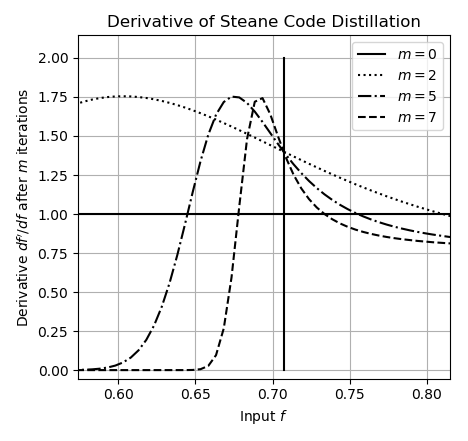
Points in the Julia set are unstable in the sense that a small perturbation can move them into the Fatou set, and cause them to converge upon distillation. This means a small change in should cause a large change in , which is easily measured using a vector derivative. To illustrate we first consider motion in the one-parameter family under the Steane code:
| (6) |
Fig. 3 shows the derivative of iterations of the Steane code. We see that the derivative peaks near the distillation threshold, and that the peak moves closer to the threshold as the code is iterated more often. Thus the derivative serves as a crude numerical means to identify the distillation threshold. In the limit of infinite , the distillation curve should be a step function, and its derivative a -function which is zero everywhere except at the threshold.
We generalize this idea to 3D via the directional derivative via a small perturbation . The directional derivative of -repeated application of , written , in a direction orthogonal to the Julia set should approach a -function.
Here is the Jacobian, and is a unit vector representing the direction of differentiation. To choose the such that the derivative is maximized, we take the largest singular value of . This is conveniently encoded by the norm: .
We demonstrate the successes and weaknesses of this technique in an interesting region of the five qubit code (5) (see Fig. 4). Observe that the large region that converges to the maximally mixed state has small since it is in the Fatou set. However the region that converges to pure states has oscillation in its output state as a function of input state. Thus is large in this entire region.


Are these points in the Fatou set or in the Julia set? The uncertainty stems from the fact that only a finite number of iterations was used in the visualization. In fact, this region has fine structure with infinitely many slim bands in the Julia set, separating by the Fatou set. Since a Julia set has no interior [Beardon], contiguous regions with high suggest such fine structure. Furthermore, is only an approximation to the Julia set when : it may be nonzero outside the Julia set and is only maximal close to the Julia set (see Fig. 3).
In this section we showed how to highlight output states via colors and how to approximate Julia sets via . As an example we demonstrated the fractal properties of the five qubit code. In the next sections we show how analyzing these fractals can benefit distillation protocols.
II Distillation thresholds
There are many advantages to restricting to the one-parameter families (1, 2), which is why many studies, e.g., [bk04], [cb-struct], [bravhaah], [jones], make the simplification. Not only does it make analysis easier, but it is motivated by the computational capabilities of the model. Magic states are eigenstates of Clifford operations:
| (7) |
This allows any qubit state to be projected into the one-parameter families via a ‘twirling’ operation, (where is some qubit Clifford gate and ):
| (8) |
| (9) |
Twirling is in principle possible in the model by applying a Clifford operation at random. Therefore restricting to one-parameter families is completely feasible.
On the other hand, if Bloch vector length is viewed as a measure of ‘purity’ of a quantum state, the twirling operations actively reduce purity and thus fidelity as a magic state. It is therefore almost surprising that distillation protocols achieve such fast distillation speeds and nearly tight thresholds with this simplification. In this section we illustrate that the five qubit code can only distill certain states if twirling is not used. We also show that twirling provides a limited view of the Steane code that may be an issue when considering noise.

The five qubit code achieves the best known distillation threshold for distilling states in the family. Unlike the Steane code for states, the five qubit code is not tight for the family. As shown in Fig. 5 there is a small gap of states outside the polytope that converge to the maximally mixed state. This shortcoming manifests itself as a slim polyhedron of states (Fig. 6) for which no successful protocol using twirling is known.
However, if we consider a cross-section of the Bloch sphere that intersects this otherwise undistillable polyhedron and plot the convergence under iteration of the five qubit code, we see that there do in fact exist distillable states inside this region (Fig. 7). This result is not completely new: it was pointed out by Reichardt [R06] who gave several examples of codes that cut into this region. However it was not realized that the curves describing the boundaries of the region were in fact a part of a fractal. It is therefore probably impossible to describe this boundary analytically.

Our current understanding of low-threshold distillation is unsatisfactory. Resource theories [resource] [monotone] strongly suggest (but do not prove) that every non-stabilizer state should be distillable to a magic state at least in principle. But we have no techniques for constructing codes with low thresholds other than guesswork. The fractal nature of distillation codes may explain why no better techniques are known: thresholds, which are essentially Julia sets, are fundamentally difficult to tailor.
Even the simplified picture of best known thresholds using twirling (Fig. 6) is misleading. There exist codes that can penetrate into the region of otherwise undistillable states. But furthermore, the one-parameter simplification provides no direct means for analyzing the stability of protocols to noise other than depolarizing noise (mixing with ). For example, the Steane code achieves tight distillation of the family, thereby distilling the vast majority of non-stabilizer mixed states. If we however plot the Julia set in a surrounding region (Fig. 8) we see that distillation is not stable: small perturbations can cause distillation to converge to a stabilizer state. This situation is reminiscent of Fig. 4.
In particular, if we simplify the Steane code polynomials governing distillation according to eqn. (3) with and assume is small so we can drop terms and higher powers, we obtain:

So already at first order Steane code distillation is unstable to perturbations in . The situation for larger deviations is best understood via the numerics in Fig. 8.
Restriction to the and families is a simplification with many merits. But when studying distillation thresholds, it paints an incomplete picture. Finding distillation protocols for all non-stabilizer states will require analysis of fractals with unpredictable properties.
III Distillation rates
The number of low-fidelity states required to assemble a target state scales exponentially in the number of repeated distillations . For practical distillation protocols it is essential that is made as small as possible. It was shown in 2009 [cb-struct] that all distillation protocols can be transformed into the standard form described at the beginning of section I. Despite this, protocols designed for distillation with low are not usually designed in this form.
Instead, quantum circuit techniques for assembling magic states using ideal resource state are combined with quantum error correction codes. A state Clifford-equivalent to the state:
| (10) |
can be used to implement a gate via a CNOT and a projection onto . Using an code where a physical acts like a logical , an approximate gate is applied to to obtain an approximate (figure ). This technique was proposed by Bravyi and Haah in [bravhaah].