Fused Segmentation of Geometric Models for Myocardium and Coronary Artery via Medial Axis
Abstract
Coronary arteries and their branches supply blood to myocardium. The obstruction of coronary arteries results in significant loss of myocardium, called acute myocardial infarction, and the number one cause of death globally. Hence, quantification of the regional amount of heart muscle subtended by obstructed coronary arteries is of critical value in clinical medicine. However, the conventional methods are inaccurate and frequently disagree with clinical practices. This study proposes a novel algorithm to segment regional myocardium-at-risk subtended by any potentially obstructed coronary artery. Assuming the geometric triangular mesh models of coronary artery and myocardium derived from an individual cardiac computed tomography image, the proposed algorithm performs (i) computation of the medial axis of the coronary artery and (ii) segmentation of the coronary artery and myocardium using the medial axis. The algorithm provides the fused segmentation of coronary artery and myocardium via the medial axis. The computed result provides a robust mathematical linkage between myocardium-at-risk and supplying coronary arteries so that ischemic myocardial regions can be accurately identified, and both the extent and severity of myocardial ischemia can be quantified effectively and efficiently. Furthermore, the correspondence between segmented coronary artery and myocardium can be more importantly used for building optimization models of cardiac systems for various applications. We believe that the proposed algorithm and implemented VoroHeart program, which is freely available at http://voronoi.hanyang.ac.kr/software/voroheart, will be an invaluable tool for patient-specific risk predictions and the treatment of obstructed coronary artery disease in clinical medicine. The algorithmic accuracy and efficiency are theoretically asserted and experimentally verified.
Keywords:
segmentation, medial axis, geometric mesh model, coronary artery, myocardium, cardiac computed tomography1 Introduction
Coronary artery disease is the number one cause of death worldwide and entrusts a huge socio-economic burden on the nations. World Health Organization 2012 statistics reported that 7.4 million people died from coronary artery disease every year [1]. Atherosclerotic obstruction of coronary artery (CA) leads to loss of oxygenated blood supply to regional myocardium (heart muscle), which causes severe myocardial ischemia and acute myocardial infarction, i.e., a heart attack.
Localizing and assessing the extent of regional myocardium-at-risk subtended by obstructed CA is of critical importance in the diagnosis and decision of treatment [2]. A 17-piece myocardial model based on two-dimensional images is currently used by clinical guidelines as recommended by the American Heart Association [3]11 1 The 17-segment model popular in medicinal community is not used here to avoid the confusion with the segmentation of data.. However, the model does not reflect individual structural variation of both CA and myocardium and frequently produces inaccurate assignments or disagreements between supplying CA and regional myocardium receiving blood [4, 5]. The establishment of an accurate and robust linkage between myocardial territory and supplying CA is required for the optimal diagnosis and treatment of CA disease [6].
Assuming that the triangular mesh model representation derived from an individual cardiac computed tomography image is available, this study presents a method to segment a myocardial 3D geometric model of a triangular mesh so that ischemic myocardial region can be accurately identified for each individual patient and both the extent and severity of myocardial ischemia can be quantified effectively and efficiently. Nowadays, many programs are frequently used to extract the geometric model of a triangular mesh from computed tomography images [7, 8, 9]. There are two driving forces, which will be detailed in Sec. 6.2, for the proposed research:
- 1.
- 2.
Figure 1 shows the overview of the approach taken by the proposed research. Given a cardiac computed tomography (cardiac CT) in the left of the figure, both CA and myocardium are derived and represented by three-dimensional geometric models of a triangular mesh [17, 18]. Given 3D geometric models in the yellow box, the method computes the medial axis of the coronary arteries in the red circle and then performs the fused segmentation of the coronary arteries and myocardium in the blue box using the medial axis. The VoroHeart program, which implemented the proposed algorithm, is freely available at http://voronoi.hanyang.ac.kr/software/voroheart. Readers are recommended to refer to the demo video for the details of VoroHeart’s functions.

Figure 2(a) shows a cardiac CT image from which the three-dimensional geometric mesh models of Figs. 2(b) through (f) are extracted. The human heart consists of four chambers (i.e., two atriums and two ventricles), valves, CA, and proximal ascending aorta. The entire heart structure is surrounded by pericardial fat (PF) as shown in Fig. 2(b). Figure 2(c) shows CA, ascending aorta, left ventricle (LV), right ventricle (RV), and left atrium (LA) after the PF, right atrium, and pulmonary artery are removed from the heart structure. Figure 2(d) shows LV, aorta, and CA that consists of left CA (LCA) and right CA (RCA), both connected to the aorta. Figure 2(e) shows CA and LV which play a key role in cardiac function. Figure 2 (f) show LV from a different view.
The statistics of the heart model in Fig. 2, which is obtained from a teaching university hospital in Korea, are as follows. Let and be the geometric models of a triangular mesh for the coronary artery and left ventricle, respectively. Similarly, let , , and be the mesh models for right ventricle, left atrium, and pericardial fat, respectively. Let and denote the number of vertices and faces of , respectively. Then , , , , , , , , , and .


We discuss a geometric method to segment myocardial region of the left ventricle (LV) into subregions, where each corresponds to a coronary artery CA piece and/or a concatenation of consecutive downhill pieces of CA. In this study, CA is modeled as a closed 2-manifold triangular mesh of a single shell with neither a mesh boundary nor a handle. This implies that CA is represented by a mesh surface with neither wall thickness nor any void. LV is also similarly modeled, yet it is interpreted to possess a thickness corresponding to the heart wall, which should be inferred from the distance between the appropriate triangular faces in the neighborhood (See Fig. 2(f)).
The remainder of this paper is organized as follows: Section 2 reviews related studies. Section 3 presents an algorithm for extracting an adjacency tree from an adjacency graph, which is constructed from a constrained Delaunay triangulation of the coronary artery. Section 4 presents the medial axis computation by refining the adjacency tree. Section 5 presents the segmentation of the left ventricle and coronary artery. Section 6 presents the algorithm summary and experimental result. Section 7 concludes the paper.
2 Literature review
This study discusses the segmentation of 3D geometric mesh models derived from cardiac CT images for the left ventricle and coronary artery using the medial axis of the coronary artery. The paper discusses two technical issues: (i) the medial axis of coronary artery and (ii) the segmentation of coronary artery and left ventricle using the medial axis that establishes their correspondence. We thus review these two issues, i.e., medial axis computation and the segmentation of image or mesh.
The medial axis, sometimes called the symmetric axis or skeleton [19], was first introduced by Blum in 1967 in order to describe biological shapes [20] and was extensively used for diverse applications such as shape description/matching [21, 22, 23], surface reconstruction [24, 25], animation [26], smoothing or sharpening of shape [27], motion planning [28], and mesh generation [29, 30].
Voronoi diagram (VD) and its dual Delaunay triangulation (DT) is one of the most fundamental tool for shape analysis and spatial reasoning. VD and DT has many applications such as coverage maximization of wireless sensor network (WSN) [31], deployment schemes for sensor coverage in WSN [32], analysis of data collected from WSN [33], and facility location [34], etc. It is known that a medial axis for a planar shape can be correctly and efficiently computed using the Voronoi diagram of a simple polygon [19, 35] which can also be used for the offset computation of the polygon by representing the Voronoi edges with rational quadratic Bzier curves [36, 37]. On the other hand, its counterpart in 3D, called a medial surface, may contain both surface patches as well as degenerating curves [25, 38], thus leaving its computation a challenge. Culver et al. presented an algorithm and its implementation for polyhedra using exact arithmetic [39]. However, the algorithm turned out impractical due to the enormous computational requirement to compute the correct medial axis with polyhedra of even a moderate size of hundreds of faces due to the algebraic complexity of the medial axis. Another important issue related with the exact computation approach is that a medial axis can have many insignificant parts related with a tiny disturbance of polyhedron geometry because the medial axis is very sensitive to perturbation [40, 41]. Therefore, an approximation approach is sufficiently justified.
An obvious approach to the approximation of a medial axis might be first to compute the Voronoi diagram of points on a model boundary and then to remove the insignificant parts of the Voronoi diagram [42, 43, 44]. This approach seems reasonable as Brandt showed in 2D that the Voronoi vertices inside the shape boundary converges to its medial axis as the sampling rate increases [45]. However, practical consideration of the trade-off between the computational requirement and solution quality due to the number of sampling points on the model boundary becomes a major bottleneck of this approach. Attali and Montanvert proposed an approximation algorithm of a 3D medial axis using the Voronoi diagram of intersection points of 3D spherical balls, which approximates the shape [42].
Based on the research experience of both segmentation of images [46, 47, 48, 49, 50] and segmentation of mesh models [51, 52, 53], the segmentation of myocardium and blood vessel was intensively studied. While several image-based studies were reported [54, 55, 56, 57, 12, 58, 59], one noteworthy work was to segment the computed tomography image of the left ventricle LV using that of the coronary artery CA, where a user manually picks some voxel points belonging to CA so that each voxel of LV can be assigned to its closest picked point [12, 60]. An application of the medial axis based on an image-based approach was reported for analyzing the morphometry, such as diameters and branching pattern of CA [61].
An improvement was made to take advantage of the mesh representation of geometric modeling. For the segmentation of myocardial mesh in 3D, a notably improved algorithm was reported that combined two representations [62], i.e., image and mesh: i) For CA, tomographic image representation - The centerline was computed via an image processing technique including the identification of branch points [63], which was then projected to the surface of LV mesh; ii) For LV, mesh representation - The Voronoi diagram of the projected points on the LV surface was computed with the geodesic distance metric so that the collection of the Voronoi cells belonging to the projection of the voxels of a particular artery piece could provide the segmentation information of LV.
3 Extraction of the adjacency tree for the coronary artery
This section explains an algorithm to extract an adjacency tree from an adjacency graph, which is constructed using a constrained Delaunay triangulation of the coronary artery . We will transform the adjacency tree to the medial axis of the , which is a one-dimensional curve-skeleton [64, 65].
3.1 Constructing the adjacency graph from constrained Delaunay triangulation
The medial axis of a simple polygon in the plane is a subset of the Voronoi diagram of the polygon [19, 35]. Figures 3(a) and (b) show the correct medial axis of a simple polygon and the (interior) Voronoi diagram of the polygon, respectively. Consider a reflex vertex in Fig. 3(b) where the internal angle between the incident edges is greater than 180 degrees. Removing Voronoi edges incident to all reflex vertices reduces the Voronoi diagram to the correct medial axis [35, 37].
However, this idea cannot be directly applied to the three-dimensional counterpart because the correct Voronoi diagram of a polyhedron is difficult to compute in general [39]. Instead, an obvious and direct approach might be to use the ordinary Voronoi diagram of sampling points on the shape boundary, as this type of Voronoi diagram can be easily computed. Then, a medial axis approximation can be obtained by a postprocessing of pruning the insignificant substructure of the Voronoi diagram.
The proposed algorithm is based on the constrained Delaunay triangulation (CDT) which is the dual structure of the constrained Voronoi diagram (Note that the Delaunay triangulation is the dual of the ordinary Voronoi diagram of points) [66, 67]. The idea is explained by the same figure. Figure 3(c) shows CDT for point generators on shape boundary where the point set contains some sampled points (i.e., the filled rectangles) in addition to the vertices of the polygon. Figure 3(d) shows the adjacency graph, which represents the adjacency among the triangles of CDT by connecting the centers of the circumcircles of triangles (See Definition 1). Note that three dotted circumcircles do not contain any other point generators, thus leading to the Delaunay property. Figure 3(e) shows the adjacency graph on the top of the medial axis. Observe that the adjacency graph relatively well approximates the medial axis. The main idea of this study for the three-dimensional medial axis starts from this simple yet important observation.


The algorithm of CDT in three-dimensional space was reported [68, 69, 70] and its well-known implementation is available [71, 72, 73]. Let be the CDT of the geometric mesh model for coronary artery where , , , and are the sets of vertices, edges, faces, and tetrahedral cells of the triangulation, respectively.
Definition 1
(Adjacency graph ) Let be the adjacency graph (adj-graph) of where and are the sets of nodes and links, respectively. Then is in one-to-one correspondence to , and the coordinate of the circumsphere center of becomes the attribute of . Two cells , are defined to be adjacent to each other if and share a common triangular face. Then each pair of adjacent cells in defines .
has the following properties.
- 1.
may have cycles.
- 2.
may have one or more nodes located outside the model boundary.
The construction of an adj-graph is obvious. Given , suppose that has adjacent cells (i.e., has neighboring cells where and each cell share one of its face with ). If the triangulation is stored in the data structure, such as the simplicial complex data structure [74], the traversal from a cell to its adjacent cell take time in the worst case. As there are adjacency relationships for CDT with triangular faces, the construction of the adj-graph can be done in linear time with respect to the number of tetrahedral cells in .
3.2 Extracting the adjacency tree from the adjacency graph by removing cycles
As the overall topology of the coronary artery is a tree, the corresponding medial axis should also be a tree. However, an adjacency graph adj-graph may have cycles depending on the arrangement of cells in the constrained Delaunay triangulation. We should remove the cycles to reduce an adj-graph to a tree.
Definition 2
(Adjacency tree ) The adjacency tree (adj-tree) corresponding to an adjacency graph (adj-graph) of is a connected subgraph of without any cycles where , .
The adj-tree may not be unique because there are in general multiple ways to remove cycles of a graph. Computing the shortest path tree (SPT) of an adj-graph, for example using the Dijkstra algorithm [75], might be a simple yet effective approach. To launch the SPT algorithm, it is necessary to determine the root node from which the entire tree can be constructed. While determination of the root node in reality requires information beyond geometry, an observation is that the shape of becomes narrower as it approaches an end tip. This implies that the root node tends to be most volumetric among the cells in . Hence, in the automatic mode, we define the root node as the cell with the largest face in the entire triangulation. We also have an additional mode to manually select the root node.
Figure 4(a) shows a schematic diagram for and its ideal medial axis. Assuming that the node in the northernmost tip is the root node , the adj-tree can be extracted with the Dijkstra algorithm by finding the shortest path from to each node of the corresponding adj-graph. However, the computed shortest path tree can be problematic in that it can be somewhat different from the ideal medial axis. It turns out that the branching node of the shortest path tree moves closer to the root node. Figures 4(b) and (c) show that this problem indeed occurs and the choice of another node as the root does not solve the problem, respectively. As the tree can branch off at a node closer to the root than at the desirable node, this phenomenon is called a of the shortest path tree. In real models, the premature branching can be of significance as shown in Fig. 5. The zoom-up shows that the tree branches off at a node much closer to the root node than at the node where it actually should.


Let the shortest path tree above be the forward shortest path tree computed by the forward pass of Dijkstra. Each shortest path is called the forward shortest path. In order to avoid premature branching, we modify the forward shortest path tree as follows. Suppose that there are leaf nodes in and thus paths from the root node. We store the paths in the priority queue according to the path length in non-increasing order (i.e., the root of corresponds to the longest path in ). Each node of also stores the leaf node of each path of .
Figure 6(a) shows for where the root (black filled circle) and leaf (unfilled circle) nodes are shown. Let be the forward shortest path corresponding to the root of , which is the longest path of from the root node to a leaf node, say . Let be the initial adj-tree, where and denote the sets of all nodes and all links in , respectively. Figure 6(b) shows . For the next iteration, is updated by removing its current root.
Consider corresponding to the next root of , which is the second longest path of from to another leaf node, say . Then we compute the shortest path of adj-graph from to by applying the Dijkstra algorithm in a backward fashion. The topological distance from a node to a tree is stated in Definition 3 below. We grow to by concatenating to (Definition 4 below states the concatenation of a tree and a path). Figure 6(c) illustrates the construction of .
The next root of corresponds to the third longest path, say from to the leaf node, say . Then we compute the shortest path from to and concatenate it to to produce . Figure 6(d) illustrates . We repeat this process while the priority queue is non-empty (See Figures 6(e) and 6(f)). The above each shortest path is called the backward shortest path and each shortest path tree is called the backward shortest path tree computed by the backward pass of Dijkstra. Figure 6(f) shows the final backward shortest path tree computed from Fig. 6(a).
Definition 3
(Distance between a node and a subtree) Suppose . The topological distance between a node and a tree is given as
| (1) |
where is the topological distance between and an arbitrary node through the shortest path between them.
Definition 4
(Concatenation) Given a tree and a path , the concatenation is defined as the addition of the nodes and links of to and , respectively.
Definition 5
(Intermediate adj-tree) Each subtree defined by the concatenations of a set of paths is an intermediate adj-tree.
Note that Eq. (1) prevents premature branching because the distance is now defined from each leaf node to the intermediate adj-tree rather than from the root node.
Let be a backward shortest path from the leaf node of adj-graph , which corresponds to the current root of at the -th step. Then the following lemma holds.
Lemma 1
(Construction of adj-tree by concatenation)
| (2) |
Be aware that can be different from and the processes in the following sections are based on .


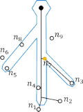
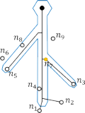

The proposed tree extraction algorithm is summarized in Algorithm 1. The code chunk line 1 through 6 computes the forward shortest path tree and stores both the leaf nodes and the corresponding paths in the priority queue. Line 7 constructs the initial adj-tree . Lines 8 through 14 iteratively update the subtree by concatenating a backward shortest path from a leaf node to the previous intermediate adj-tree. Note that line 11 implies that the length of a backward path can be zero when the leaf node for is already included in any previously updated subtree. For example, a leaf node is included in the backward shortest path as shown in Fig. 6(d). The length of the backward path from is zero, thus is not concatenated any more.
The Dijkstra algorithm takes time in the worst case if it is based on a priority queue implemented by a Fibonacci heap where and represent the numbers of nodes and links, respectively [76]. Note that the Dijkstra algorithm can deteriorate to time in the worst case if it is implemented otherwise. The proposed algorithm runs two passes of Dijkstra: one for the forward pass and the other for the backward pass. The forward pass computes the shortest paths of all nodes from the root, whereas the backward pass consists of the runs for computing the backward shortest path from each leaf node to an intermediate adj-tree. Hence, the worst-case time complexity of Algorithm 1 becomes using a Fibonacci heap.
4 Transformation of adjacency tree to medial axis
The adjacency tree adj-tree above becomes the initial representation of the medial axis, which is fine-tuned in this section.
4.1 Removing outrageous nodes
The medial axis of a shape should be located inside the shape boundary. However, the adj-tree obtained in the previous section may have some extraneous nodes that are placed outside the geometric mesh model of the coronary artery. Figure 7 shows and the corresponding adj-tree. As shown in the close-up, the adj-tree has several blue leaf nodes emanating to the outside of . This section presents an algorithm to remove those extraneous nodes.

Definition 6
(Outrageous node) Given an adj-tree , if is placed outside , is called an outrageous node and the corresponding CDT cell is called an outrageous cell.
It turns out that an outrageous cell tends to be relatively flat and is located near the boundary of [43]. Figure 7, in the close-up, shows some (blue) outrageous nodes and the corresponding (red) flat cells near the boundary. We will remove those nodes from via two steps as follows: (i) Identify the outrageous nodes and (ii) remove those nodes.
A simple yet effective way to identify the outrageous nodes is to check if the intersection between links and the boundary of . Consider a link whose start node is inside . The end node of the link will be inside if does not intersect or has an even number of intersections. On the other hand, the end node will be outside if has an odd number of intersections. Mostly, the number of intersections will be less than two. If we pick the links incident to the end node, this process can be repeated because we have always one visited node (a node whose status is known) and the other unvisited node for each link. After all nodes are visited, all of the outrageous nodes are recognized.
After identifying the outrageous nodes, we traverse the adj-tree, starting from an outrageous leaf node, and collect the outrageous nodes until we cross the boundary. Then we remove the collected nodes safely. The bucket system is exploited in order to localize the candidate faces of for the intersection. Assuming that the number of candidate faces for the intersection of each link is , the algorithm takes time in the worst-case scenario where is the number of nodes of adj-tree.
4.2 Shaving hairs
The adj-tree after the removal step usually contains tiny subtrees that constitute an undesirable part of the medial axis. Such a subtree is called a because its contribution to a medial axis is negligible. In this section, we discuss an operation to remove hairs, called . Figures 8(a) and (b) show the adj-tree before and after shaving the (yellow) hairs, respectively.


We measure the contribution of each subtree, say , of an adj-tree to the corresponding medial axis as follows. Given an intermediate tree , consider adding a subtree to to produce . If the contribution of is significant, it is is considered a new subtree of . Otherwise, we consider it a hair.
Definition 7
(Distance between trees) The distance between two trees and where is
| (3) |
| (4) |
where is the topological distance between and as defined in Eq. (1).
Note that if and only if . If , . Hence, can be an indicator that tells us how close the intermediate adj-tree is to .
Hence, is non-increasing and . Lemma 2 states that an intermediate adj-tree is closer to the original adj-tree as we concatenate more paths. However, the marginal increase of the closeness of each incrementally concatenated path should be investigated since that of one path can be significantly different from that of another. We evaluate for each root, say in the -th iteration, of a priority queue , which corresponds to a path in . is concatenated to if , where is a parameter given by the user.
The proposed hair-shaving algorithm is summarized in Algorithm 2. Lines 1 through 5 compute the path from the root node to each leaf node and store each path and its corresponding leaf node in the priority queue according to a non-increasing order of path length. Lines 6 through 15 compute the distance of each intermediate adj-tree which is constructed by concatenating each path. Then of Eq. (4) is also computed. Lines 12 through 14 incrementally construct the shaved adj-tree. Note that line 13 concatenates a path to the current shaved tree only if the distance reduction induced by is larger than a given threshold . In this study, we have used the average distance reduction of intermediate adj-trees for . Algorithm 2 takes time in the worst-case scenario, where is the number of nodes in the unshaved tree.
4.3 Straightening bumpy nodes
The adj-tree after the outrageous node removal step may still have some outrageous nodes, which need to be somehow fixed to improve the quality of the adj-tree to be the medial axis. As a brute force removal of such a node may cause a disconnectedness of the adj-tree, it should be carefully managed. This section presents an algorithm to remove those nodes outside so that the adj-tree is a connected component.
Consider four consecutive nodes , and of an adj-tree, and their associated three links , and . Each link is defined by two consecutive nodes and . Then we may define the unit direction vectors , and corresponding to , and , respectively. Consider the difference vector . Then shows how far node is away from neighboring nodes. A similar interpretation can be applied to for node . Consider the following two conditions.
| (6) | |||
| (7) |
where and are some threshold. Satisfying both of the conditions means that node is relatively far away compared to node (Refer to B for an alternative interpretation of Eqs. (6) and (7)). Then, it would be reasonable that the bumpy node and both links and are removed from the adj-tree and a new link connecting and is inserted. The proposed algorithm removes those nodes and associated links and inserts new links by checking the above conditions. In this study, we have chosen 0.5 for both and through some experiments. It turns out that the algorithm effectively smooths down by straightening the bumpy nodes (See Figs. 10 (c) and (d) to compare the adjacency tree before and after straightening bumpy nodes).
5 Fused segmentation of ventricles and arteries
This section presents the segmentation of the geometric mesh models and for left ventricle and coronary artery, respectively, using the above computed medial axis of . Once is available, the segmentation can be done in a rather simple way. We first present the segmentation of in detail and then present that of , which is similar to but simpler than that of .
5.1 Segmenting left ventricle
Given the medial axis , the algorithm will segment into a set of subregions so that each subregion is assigned to one and only one node of .
Suppose that the constrained Delaunay triangulation of is available. Let be the nodes of . Then, we can formulate the segmentation of as a problem to assign each cell of to one and only one node of so that the summation of the distance between each cell and each node is minimized. We use the Euclidean distance between the mass center of the cell and the coordinate of the medial axis node while other considerations such as the radii of CA, blood stream flow, and blood pressure may have to be reflected in future.
The segmentation of is a many-to-one assignment problem that can be formulated as an integer linear program as follows:
| (8) | |||||
| (9) | |||||
| (10) |
where and are the index sets which label the elements of and , respectively. the distance between the mass center of and . Equation (9) forces each cell to be assigned to one and only one node. The formulation above can be solved by an implementation which, taking time in the worst-case, assigns to the node which corresponds to
| (11) |
The definition of the distance in Eq. (11) can be improved by reflecting the medical condition, and the efficiency improvement needs to be made in the future.
5.2 Segmenting the coronary artery
The segmentation of is similarly done by assigning each tetrahedral cell of the constrained Delaunay triangulation of to a node of according to the minimum Euclidean distance. Note that is already available during the computation of . Then the algorithm segments both left and right by assigning each cell of s to a node of .
Figure 9 shows the segmentation result. Figure 9(a) shows the medial axis of both left coronary artery () and right coronary artery () is computed and their branches are also recognized: The branches of are red-colored while those of are blue-colored. Figures 9(b) and (c) show the segmentations of and with the colors synchronized, respectively. Figure 9(d) shows the segmented and altogether from a different orientation. Recall that we model left ventricle with a wall thickness: Be aware that the myocardium inside is also segmented and thus the volume of myocardial region corresponding to a supplying coronary artery piece can be measured.


6 Algorithm summary and experiments
This section summarizes the proposed algorithm and presents experimental results on both the segmentation of the coronary artery and left ventricle and computation of the medial axis.
6.1 Algorithm summary
The proposed algorithm is summarized in Algorithm 3, which first computes the constrained Delaunay triangulation of . Then an adjacency graph is constructed from in Step 2. Step 3 extracts an adjacency tree by removing the cycles of the adjacency graph. The adjacency tree is transformed to the medial axis by removing outrageous nodes, shaving hairs, and straightening bumpy nodes in Steps 4, 5, and 6, respectively. Step 7 computes for the segmentation of . Then the algorithm segments and into subregions by assigning each tetrahedral cell in both and to each node in the medial axis in Steps 8 and 9, respectively.
Figure 10 shows the computation results for Steps 3, 4, 5 and 6 of Algorithm 3 using the close-up of the adjacency tree and coronary artery. Figures 10(a) and (b) respectively show the adjacency trees before and after outrageous nodes are removed. In both figures, the adjacency tree is superimposed on the boundary of the coronary artery mesh. Figures 10(c) and (d) show the adjacency trees only after the shaving and straightening, respectively.


6.2 Experimental results
Algorithm 3 was implemented using the Microsoft Visual C++ and OpenGL library. Figure 11 shows the developed VoroHeart program running on Microsoft Windows. After segmenting and using , VoroHeart visualizes the recognized branches of in the main pane with the synchronized colors for the corresponding and segments. The right pane displays the tree hierarchy of branches and the lower pane shows the parent-and-child relationship between branches with a color-encoding. The lower pane also shows the mass properties of each segmented subregion of and its supplying branch. The mass properties include the volume/surface area of the segmented subregion, the length, thickness, surface area, and volume of branch, of which the importance for medical diagnosis and treatment to the cardiac function was verified [11, 12, 13]. Hence, the VoroHeart program, which implemented the proposed algorithm, will be useful for the assessment of the severity of heart attack by quantifying the volume and area of the myocardium-at-risk.

Figure 12 shows an application using segmentation of the left ventricle. Suppose that we pick a point, as marked by the yellow arrow, which actually corresponds to a node of the medial axis of . Consider that the coronary artery is obstructed at the picked point. Figure 12(a) shows i) the subset of the coronary artery from the pick point down to the leaves (shown in light gray), and ii) the subset of the myocardial muscle corresponding to the coronary artery subset (shown in dark gray). Figure 12(b) shows the case that the picking point is located further down to a leaf. Observe that the corresponding myocardial muscle region shrinks.


Figure 13 shows a section view of the left ventricle and the entire coronary arteries. Figure 13(a) shows the remaining part of the left ventricle after the upper ventricular lump above a trimming plane is removed where the trimming plane (not shown in the figure) is created through a user-interaction with VoroHeart via the screen. The figure in the red-box of Figure 13(a) is the ventricle from a different view. Be aware that the muscle in the ventricle wall is also properly assigned to a corresponding branch. Figure 13(b) similarly shows a section view for a different trimming plane. Thus we can investigate the morphometry of myocardium such as the wall thickness from the section view and can easily compute the thickness if necessary. Note that the wall thickness of the left ventricle is an important measure for analyzing cardiac function and diagnosing cardiovascular disease [77, 78, 79].
Thus, the proposed geometric model based approach can facilitate various clinical studies where model quantification is an important measure [10, 11, 12, 13, 80]. Furthermore, the proposed research could be exploited for applications related to model optimization. For example, one of the promising therapies for cardiac disease is to transplant stem cells into either the myocardium at the site of injury or the supplying CA branch [15, 16]. One important issue for this approach is to optimize the delivery of stem cells to the appropriate site so that cardiac regeneration is maximized [14]. In this case, the segmentation result of this study would be more importantly used for the delivery optimization.


We have also tested Algorithm 3 using a data set of 20 clinical cases of anonymous patients from a teaching university hospital in Korea. The cardiac CT image of each case for left and right coronary arteries and left ventricle was obtained using a dual source CT scanner, SOMATOM Definition Flash (Siemens Healthineers, Germany) [81] with a slice thickness 0.6mm and nonionic contrast medium (iomeron), in DICOM (Digital Imaging and Communications in Medicine) format [82]. The geometric model stored in the STL format was extracted from an individual cardiac CT image using the VitreaWorkstation program [7]. The computational environment for the experiment is as follows: CUP: Inter Core2 Duo E7500 2.93Ghz; RAM: 4GB; OS: Windows 7.
Figure 14 shows the size of the input geometric mesh models for both the coronary artery (Figure 14(a)) and the left ventricle (Figure 14(b)). The horizontal axis, not only this figure but also throughout this section, represents the number of triangular faces of each input mesh model and the vertical axis the number of vertices and edges. The graphs show a strong linear relationship. Figures 15(a) and (b) show the size of s for both and , respectively. The vertical axis represents the number of vertices, edges, faces, and cells of s. The graphs are again all linear. Figure 16(a) shows the size of the adjacency graph and adjacency tree where different colors denote the entity size after different steps of the algorithm are applied. Note that the data size decreases as the algorithm proceeds in its steps for computing the medial axis. While the adjacency tree extraction and shaving steps significantly reduce the number of nodes, both the outrageous-node removing and the straightening steps do not reduce much. Figure 16(b) shows two curves corresponding to the shaving and straightening steps.


Figure 17 shows the computation time of both the medial axis and the entire segmentation for the test data set of twenty clinical cases. We group the steps of Algorithm 3 into three phases. Phase I (extraction of adjacency tree) consisting of Steps 1, 2, and 3; Phase II (transformation of adjacency tree to medial axis) consisting of Steps 4, 5, and 6; and Phase III (segmentation of ventricles and coronary arteries) consisting of Steps 7, 8, and 9. Figure 17(a) decomposes the computation time for the medial axis into three parts: the time for loading each model file, the time for Phase I, and the time for Phase II. Note that the total time shows a quadratic increase with respect to the model size because the most expensive operation is Step 3 with the time complexity with respect to nodes and links in the adjacency graph (See Sec. 3.2) and both and linearly increase regarding the model size. For the clarity of the other times, the times for Phase I and II are shown in Figs. 17(b) and (c), respectively. The time for loading the triangular mesh model is excluded. Among the times for Phase I, the time for adjacency tree extraction is mostly dominant while times for both and the adjacency graph are relatively negligible. For the steps of Phase II, the outrageous-node-removing takes more time than other steps. The bumpy-node-straightening step is relatively negligible. Figure 17(d) shows the times for the model file loading and Phase III, which consists of the computation of , -segmentation, and -segmentation. The time for is not shown because that is already included in Phase I. The time for -segmentation shows a linear increase with model size because its time complexity is with respect to nodes in the medial axis and tetrahedral cells in , respectively (See Sec. 5). Note that and linearly increases with model size. The similar argument applies to the time for -segmentation.


7 Conclusion
This study presents an algorithm and its implementation to segment regional myocardium-at-risk subtended by any potentially obstructed coronary artery based on the geometric models of a triangular mesh for the coronary artery and myocardium obtained from an individual cardiac computed tomography image. The key idea of the algorithm is (i) computation of the medial axis of the coronary artery and (ii) segmentation of the coronary artery and myocardium into a set of regions where each corresponds to a node of the medial axis. The medial axis is transformed from an adjacency tree, which is extracted by removing cycles of an adjacency graph. The adjacency graph is constructed from the constrained Delaunay triangulation of the triangular mesh model of the coronary artery. The algorithmic accuracy and efficiency are theoretically asserted and experimentally verified.
Obstruction of the coronary artery results in acute myocardial infarction. Hence, quantification of the regional amount of myocardium subtended by the obstructed coronary artery is of critical value in clinical medicine. However, conventional methods such as the 17-piece model are inaccurate and frequently disagree with clinical practice. The proposed algorithm provides a robust mathematical linkage between myocardium-at-risk and supplying coronary arteries so that ischemic myocardial region can be accurately identified, and both the extent and severity of myocardial ischemia can be quantified effectively and efficiently. Furthermore, the computed result of segmented coronary artery and myocardium can be more importantly used for building optimization models of cardiac systems for various applications. We believe that the algorithm and developed VoroHeart program will be an invaluable tool for patient-specific risk predictions and the treatment of obstructed coronary artery disease in clinical medicine.
Acknowledgments
The authors would like to thank research assistants Seon-A Jeong and So-Hyeon Park for their efforts to prepare clinical data. Jehyun Cha, Joonghyun Ryu, and Deok-Soo Kim were supported by the National Research Foundation of Korea(NRF) grant funded by the Korea government(MSIP) (No. 2017R1A3B1023591). Jin-Ho Choi was supported by grants from Samsung Medical Center basic research (GL1B33211, CRP1500053), and the Korean Society of Interventional Cardiology (2014-1).
References
References
- [1] World Health Organization, World health statistics 2012 (world health statistics annual), Tech. rep., World Health Organization (2012).
- [2] B. D. Bruyne, W. F. Fearon, N. H. Pijls, E. Barbato, P. Tonino, Z. Piroth, N. Jagic, S. Möbius-Winckler, G. Rioufol, N. Witt, P. Kala, P. MacCarthy, T. Engström, K. Oldroyd, K. Mavromatis, G. Manoharan, P. Verlee, O. Frobert, N. Curzen, J. B. Johnson, A. Limacher, E. Nüesch, P. Jüni, Fractional flow Reserve–Guided pci for stable coronary artery disease, The New England Journal of Medicine 371 (2014) 1208–1217.
- [3] M. D. Cerqueira, N. J. Weissman, V. Dilsizian, A. K. Jacobs, M. Sanjiv Kaul, W. K. Laskey, D. J. Pennell, J. A. Rumberger, T. Ryan, M. S. Verani, Standardized myocardial segmentation and nomenclature for tomographic imaging of the heart, Circulation 105 (2002) 539–542.
- [4] J. T. Ortiz-Pérez, J. Rodríguez, S. N. Meyers, D. C. Lee, C. Davidson, E. Wu, Correspondence between the 17-segment model and coronary arterial anatomy using contrast-enhanced cardiac magnetic resonance imaging, JACC : Cardiovascular Imaging 1 (3) (2008) 282–293.
- [5] M. S. Javadi, R. Lautamäki, J. Merrill, C. Voicu, W. Epley, G. McBride, F. M. Bengel, Definition of vascular territories on myocardial perfusion images by integration with true coronary anatomy: A hybrid pet/ct analysis, Journal of Nuclear Medicine 51 (2) (2010) 198–203.
- [6] B. D. Bruyne, N. H. Pijls, B. Kalesan, E. Barbato, P. A. Tonino, Z. Piroth, N. Jagic, S. Möbius-Winkler, G. Rioufol, N. Witt, P. Kala, P. MacCarthy, T. Engström, K. G. Oldroyd, K. Mavromatis, G. Manoharan, P. Verlee, O. Frobert, N. Curzen, J. B. Johnson, P. Jüni, W. F. Fearon, Fractional flow Reserve–Guided pci versus medical therapy in stable coronary disease, The New England Journal of Medicine 367 (2012) 991–1001.
- [7] Vitrea workstation, http://www.toshiba-medical.eu (2015).
- [8] Aquarius, http://www.terarecon.com (2016).
- [9] IntelliSpace Portal, http://www.usa.philips.com (2016).
- [10] S. Saito, J. Y. K. Miura, N. Nakao, T. Nagao, T. Sugimoto, T. Hirano, N. Kuroda, Y. Iimuro, J. Fujimoto, A novel 3d hepatectomy simulation based on liver circulation: Application to liver resection and transplantation, Hepatology 41 (6) (2005) 1297–1304.
- [11] S. Sumitsuji, S. Ide, P. T. Siegrist, Y. Salah, K. Yokoi, M. Yoshida, M. Awata, K. Yamasaki, K. Tachibana, H. Kaneda, S. Nanto, Y. Sakata, Reproducibility and clinical potential of myocardial mass at risk calculated by a novel software utilizing cardiac computed tomography information, Cardiovascular Intervention and Therapeutics 31 (2016) 218–225.
- [12] A. Kurata, A. Kono, T. Sakamoto, T. Kido, T. Mochizuki, H. Higashino, M. Abe, A. Coenen, R. G. Saru-Chelu, P. de Feyter, G. P. Krestin, K. Nieman, Quantification of the myocardial area at risk using coronary ct angiography and voronoi algorithm-based myocardial segmentation, European Radiology 25 (1) (2015) 49–57.
- [13] A. F.Frangi, W. J.Niessen, M. A.Viergever, Three-dimensional modeling for functional analysis of cardiac images: A review, IEEE Transzctions on Medical Imaging 20 (1) (2001) 2–25.
- [14] P. Oettgen, Cardiac stem cell therapy need for optimization of efficacy and safety monitoring, Circulation 114 (4) (2006) 339–358.
- [15] V. F. M. Segers, R. T. Lee, Stem-cell therapy for cardiac disease, Nature 451 (2008) 937–942.
- [16] M. Shafiq, Y. Jung, S. H. Kim, Insight on stem cell preconditioning and instructive biomaterials to enhance cell adhesion, retention, and engraftment for tissue repair, Biomaterials 90 (2016) 85–115.
- [17] C. Lorenz, J. von Berg, A comprehensive shape model of the heart, Medical Image Analysis 10 (2006) 657–670.
- [18] S. de Putter, F. N. van de Vosse, F. A. Gerritsen, F. Laffargue, M. Breeuwer, Computational mesh generation for vascular structures with deformable surfaces, International Journal of Computer Assisted Radiology and Surgery 1 (1) (2006) 39–49.
- [19] D. G. Kirkpatrick, Efficient computation of continuous skeletons, in: Proceedings of the 14th Annual IEEE Symposium on Foundations of Computer Science, 1979.
- [20] H. Blum, A transformation for extracting new descriptors of shape, in: W. Wathen-Dunn (Ed.), Models for the Perception of Speech and Visual Form, Cambridge, MA, 1967, pp. 362–380.
- [21] H. Blum, R. N. Nagel, Shape description using weighted symmetric axis features, Pattern Recognition 10 (1978) 167–180.
- [22] L. R. Nackman, S. M. Pizer, Three-dimensional shape description using the symmetric axis transform i: Theory, IEEE Transactions on Pattern Analysis and Machine Intelligence PAMI-7 (2) (1985) 187–202.
- [23] S. M. Pizer, W. R. Oliver, S. H. Bloomberg, Hierarchical shape description via the multiresolution symmetric axis transform, IEEE Transactions on Pattern Analysis and Machine Intelligence PAMI-9 (4) (1987) 505–511.
- [24] N. Amenta, M. Bern, M. Kamvysselis, A new Voronoi-based surface reconstruction algorithm, in: Proceedings of the SIGGRAPH ’98, 1998, pp. 415–421.
- [25] A. C. Jalba, J. Kustra, A. C. Telea, Surface and curve skeletonization of large 3d models on the gpu, IEEE Transactions on Pattern Analysis and Machine Intelligence 35 (6) (2013) 1495–1508.
- [26] L. Wade, R. E. Parent, Automated generation of control skeletons for use in animation, The Visual Computer 18 (2) (2002) 97–110.
- [27] S. beng Ho, C. R. Dyer, Shape smoothing using medial axis properties, IEEE Transactions on Pattern Analysis and Machine Intelligence PAMI-8 (4) (1986) 512–520.
- [28] C. Holleman, L. E. Kavraki, A framework for using the workspace medial axis in prm planners, in: IEEE International Conference on Robotics and Automation, Vol. 2, 2000, pp. 1408–1413.
- [29] T. Tam, C. Armstrong, 2d finite element mesh generation by medial axis subdivision, Advances in Engineering Software and Workstations 13 (5-6) (1991) 313–324.
- [30] L. Linardakis, N. Chrisochoides, Algorithm 870: A static geometric medial axis domain decomposition in 2d euclidean space, ACM Transactions on Mathematical Software (TOMS) 34 (1).
- [31] M. Abo-Zahhad, N. Sabor, S. Sasaki, S. M. Ahmed, A centralized immune-voronoi deployment algorithm for coverage maximization and energy conservation in mobile wireless sensor networks, Information Fusion 30 (2016) 36–51.
- [32] M. R. Senouci, A. Mellouk, K. Asnoune, F. Y. Bouhidel, Movement-assisted sensor deployment algorithms: A survey and taxonomy, IEEE Communications Surveys & Tutorials 17 (4) (2015) 2493–2510.
- [33] H. H. Bosman, G. Iacca, A. Tejada, H. J. W’́ortche, Spatial anomaly detection in sensor networks using neighborhood information, Imformation Fusion 33 (2017) 41–56.
- [34] F. Peng, X. Wang, Y. Ouyang, Approximation of discrete spatial data for continuous facility location design, Integrated Computer-Aided Engineering 21 (4) (2014) 311–320.
- [35] D. T. Lee, Medial axis transformation of a planar shape, IEEE Transactions on Pattern Analysis and Machine Intelligence 4 (1982) 363–369.
- [36] D.-S. Kim, Polygon offsetting using a Voronoi diagram and two stacks, Computer-Aided Design 30 (14) (1998) 1069–1076.
- [37] D.-S. Kim, I.-K. Hwang, B.-J. Park, Representing the Voronoi diagram of a simple polygon using rational quadratic Bzier curves, Computer-Aided Design 27 (8) (1995) 605–614.
- [38] W. GONG, G. BERTRAND, A simple parallel 3d thinning algorithm, in: Proc. IEEE Pattern Recognition, 1990, pp. 188–190.
- [39] T. Culver, J. Keyser, D. Manocha, Exact computation of the medial axis of a polyhedron, Computer Aided Geometric Design 21 (1) (2004) 65–98.
- [40] D. Shaked, A. M. Brucksteiny, Pruning medial axes, Computer Vision and Image Understanding 69 (2) (1998) 156–169.
- [41] S. W. Choi, H.-P. Seidel, Linear onesided stability of mat for weakly injective 3d domain, Computer-Aided Design 36 (2) (2004) 95–109.
- [42] D. Attali, A. Montanvert, Computing and simplifying 2d and 3d continuous skeletons, Computer Vision and Image Understanding 67 (3) (1997) 261–273.
- [43] N. Amenta, S. Choi, R. K. Kolluri, The power crust, unions of balls, and the medial axis transform, Computational Geometry - Theory and Applications 19 (2001) 127–153.
- [44] T. K. Dey, W. Zhao, Approximate medial axis as a voronoi subcomplex, Computer-Aided Design 36 (2004) 195–202.
- [45] J. Brandt, Convergence and continuity criteria for discrete approximation of the continuous planar skeleton, CVGIP: Image Understanding 59 (1) (1994) 116–124.
- [46] A. P. James, B. V. Dasarathy, Medical image fusion: A survey of the state of the art, Information Fusion 19 (2014) 4–19.
- [47] N. Makni, N. Betrouni, O. Colot, Introducing spatial neighbourhood in evidential c-means for segmentation of multi-source images: Application to prostate multi-parametric mri, Information Fusion 19 (2014) 61–72.
- [48] M. Mignotte, A label field fusion model with a variation of information estimator for image segmentation, Information Fusion 20 (2014) 7–20.
- [49] D. Schwarz, T. Kasparek, Brain morphometry of MR images for automated classification of first-episode schizophrenia, Information Fusion 19 (2014) 97–102.
- [50] A. Sankaran, A. Jain, T. Vashisth, M. Vatsa, R. Singh, Adaptive latent fingerprint segmentation using feature selection and random decision forest classification, Information Fusion 34 (2017) 1–15.
- [51] A. Shamir, A survey on mesh segmentation techniques, Computer Graphics forum 27 (6) (2008) 1539–1556.
- [52] O. K.-C. Au, Y. Zheng, M. Chen, P. Xu, C.-L. Tai, Mesh segmentation with concavity-aware fields, IEEE Transactions on Visualization and Computer Graphics 18 (7) (2012) 1125–1134.
- [53] Y. Zheng, C.-L. Tai, O. K.-C. Au, Dot scissor: A single-click interface for mesh segmentation, IEEE Transactions on Visualization and Computer Graphics 18 (18) (2012) 1304–1312.
- [54] J. S.Suri, Computer vision, pattern recognition and image processing in left ventricle segmentation: The last 50 years, Pattern Analysis & Applications 3 (3) (2000) 209–242.
- [55] S. C. Mitchell, B. P. F. Lelieveldt, R. J. van der Geest, H. G. Bosch, J. H. C. Reiber, M. Sonka, Multistage hybrid active appearance model matching: segmentation of left and right ventricles in cardiac mr images, IEEE Transactions on Medical Imaging 20 (5) (2001) 415–423.
- [56] N. Paragios, A level set approach for shape-driven segmentation and tracking of the left ventricle, IEEE Transactions on Medical Imaging 22 (6) (2003) 773–776.
- [57] D. Lesage, E. D. Angelini, I. Bloch, G. Funka-Lea, A review of 3d vessel lumen segmentation techniques: Models, features and, Medical Image Analysis 13 (6) (2009) 819–845.
- [58] I. Cabria, I. Gondra, Mri segmentation fusion for brain tumor detection, Information Fusion 36 (2017) 1–9.
- [59] ChaoyingTang, H. Zhang, A. Kong, Using multiple models to uncover blood vessel patterns in color images for forensic analysis, Information Fusion 32 (2016) 26–39.
- [60] H. G. Debarba, D. J. Zanchet, D. Fracaro, A. Maciel, A. N. Kalil, Efficient liver surgery planning in 3d based on functional segment classification and volumetric information, in: 32nd Annual International Conference of the IEEE EMBS, 2010.
- [61] T. Wischgoll, J. S. Choy, E. L. Ritman, G. S. Kassab, Validation of image-based method for extraction of coronary morphometry, Annals of Biomedical Engineering 36 (3) (2008) 356–368.
- [62] M. Termeer, J. O. Bescós, M. Breeuwer, A. Vilanova, F. Gerritsen, M. Gröller, E. Nagel, Patient-Specific Mappings between Myocardial and Coronary Anatomy, Vol. 1 of Dagstuhl Follow-Ups, Schloss Dagstuhl-Leibniz-Zentrum fuer Informatik, 2010.
- [63] C. Lorenz, S. Renisch, T. Schlathölter, T. Bülow, Simultaneous segmentation and tree reconstruction of the coronary arteries in msct images, Proceeding of SPIE 5031 (2003) 167–177.
- [64] L. Liu, E. W. Chambers, D. Letscher, T. Ju, A simple and robust thinning algorithm on cell complexes, in: Pacific Graphics 2010, Vol. 29, 2010.
- [65] N. D. Cornea, D. Silver, P. Min, Curve-skeleton properties, applications, and algorithms, IEEE Transactions on Visualization and Computer Graphics 13 (3) (2007) 530–548.
- [66] F. Aurenhammer, Voronoi diagrams – a survey of a fundamental geometric data structure, ACM Computing Surveys 23 (3) (1991) 345–405.
- [67] A. Okabe, B. Boots, K. Sugihara, S. N. Chiu, Spatial Tessellations: Concepts and Applications of Voronoi Diagrams, 2nd Edition, John Wiley & Sons, Chichester, 1999.
- [68] J. R. Shewchuk, Updating and constructing constrained delaunay and constrained regular tringulations by flips, in: nineteenth annual symposium on Computational geometry, 2003, pp. 181–190.
- [69] H. Si, K. Gartner, 3d boundary recovery by constrained delaunay tetrahedralization, International Journal for Numerical Methods in Engineering 85 (2011) 1341–1364.
- [70] H. Si, J. R. Shewchuk, Incrementally constructing and updating constrained delaunay tetrahedralizations with finite-precision coordinates, Engineering with Computers 30 (2014) 253–269.
- [71] H. Si, Three dimensional boundary conforming delaunay mesh generation, Ph.D. thesis, TU Berlin (2008).
- [72] H. Si, Tetgen: A quality tetrahedral mesh generator and 3d delaunay triangulator, Technical Report 13, WIAS (2013).
- [73] H. Si, Tetgen, a delaunay-based quality tertrahedral mesh generator, ACM Transactions on Mathematical Mesh Generator 41 (2) (2015) Article No. 11.
- [74] D.-S. Kim, D. Kim, Y. Cho, K. Sugihara, Quasi-triangulation and interworld data structure in three dimensions, Computer-Aided Design 38 (7) (2006) 808–819.
- [75] E. W. Dijkstra, A note on two problems in connexion with graphs, Numerische Mathematik 1 (1959) 269–271.
- [76] M. L. Fredman, R. Tarjan, Fibonacci heaps and their uses in improved network optimization algorithms, in: 25th Annual Symposium on Foundations of Computer Science, 1984, pp. 338–346.
- [77] S. Sasayama, D. Franklin, J. R. Jr., W. S. Kemper, D. McKown, Dynamic changes in left ventricular wall thickness and their use in analyzing cardiac function in the conscious dog: A study based on a modified ultrasonic technique, The American Journal of Cardiology 38 (7) (1976) 870–879.
- [78] W. H. Gaasch, Left ventricular radius to wall thickness ratio, The American journal of cardiology 43 (6) (1979) 1189–1194.
- [79] I. Olivotto, R. Gistri, P. Petrone, E. Pedemonte, D. Vargiu, F. Cecchi, Maximum left ventricular thickness and risk of sudden death in patients with hypertrophic cardiomyopathy, Journal of the American College of Cardiology 41 (2) (2003) 315–321.
- [80] S. Prakash, C. R. Ethier, Requirements for mesh resolution in 3d computational hemodynamics, Journal of Biomechanical Engineering 123 (2001) 134–144.
- [81] Siemens Healthineers, https://www.healthcare.siemens.com (2016).
- [82] Digital Imaging and Communications in Medicine, h͡ttp://dicom.nema.org/ (2015).
Appendix A Proof of Lemma 2
Proof: Given where has leaf nodes, because .
Appendix B Interpretation of the conditions in Eqs. (6) and (7)
The conditions in Eqs. (6) and (7) can be interpreted alternatively as follows. Suppose that , and are the uniformly sampled points on a smooth curve. Thus, the lengths of and are equivalent to each other. If we increase the sampling rate, the length of each link decreases. In the limiting case, each corresponding unit vector approaches the unit tangent vector of the curve and each link approaches the curve piece. Let and be the tangent vectors of the limiting case that correspond to the unit direction vectors of and , respectively. is the difference vector on between and .
Consider the osculating circle c on the node . Let and be the center and the radius of c, respectively. Let be the angle between and and let . Then following Lemma 3 says that can be represented via the radius of the osculating circle and the arc length .
Lemma 3
| (12) |
Proof: Refer to Fig. 18. The angle because is the angular bisector of . Let us draw the perpendicular line from a point on to . Then holds because is the angular bisector of where .
Because the triangle is an isosceles triangle, the angle . Consider the perpendicular line from to . Then similarly, holds because is the angular bisector of the angle . From the above equations,

Assuming that the length of each link is equal to each other and sufficiently small, i.e., , Lemma 3 shows that reflects the curvature at node well. The derivation and interpretation could similarly apply to for . Equation (7) shows how much the curvature is different between and . Therefore, the proposed algorithm for straightening bumpy nodes approximately reflects the variation of the local curvature.