跳到论文正文
W Papers独立论文阅读器 arXiv:1708.09004 论文正文 计算阅读时间 · 0%
引用这篇论文根据当前论文元数据生成,正式投稿前建议核对。


License: arXiv.org perpetual non-exclusive license
arXiv:1708.09004v1 [math.ST] 29 Aug 2017

Preliminary Testing Derivatives of a Linear Unified Estimator in the Logistic Regression Model

Yasin Asar* Yasin Asar*Corresponding Author: Department of Mathematics-computer Sciences Necmettin Erbakan University, Konya, Turkey Email address: yasar@konya.edu.tr, yasinasar@hotmail.com , Bahadır Yüzbaşı Bahadır YüzbaşıDepartment of Econometrics, Inonu University, Malatya 44280, Turkey Email address: b.yzb@hotmail.com , Mohammad Arashi Mohammad ArashiDepartment of Statistics, School of Mathematical Sciences, Shahrood University of Technology, Shahrood, Iran Email address: m_arashi_stat@yahoo.com and Jibo Wu Jibo WuKey Laboratory of Group and Graph Theories and Applications, Chongqing University of Arts and Sciences, Chongqing, China Email address: linfen52@126.com
Abstract.

Recently, the well-known Liu estimator [19] is attracted researchers’ attention in regression parameter estimation for an ill-conditioned linear model. It is also argued that imposing sub-space hypothesis restriction on parameters improves estimation by shrinking toward non-sample information. [10] proposed the almost unbiased Liu estimator (AULE) in the binary logistic regression. In this article, some improved unbiased Liu type estimators, namely, restricted AULE, preliminary test AULE, Stein-type shrinkage AULE and its positive part for estimating the regression parameters in the binary logistic regression model are proposed based on the work [10]. The performances of the newly defined estimators are analyzed through some numerical results. A real data example is also provided to support the findings.

Keywords: Biasing parameter; Logistic regression; MLE; Preliminary test estimator; Unbiased Liu estimator

2010 Mathematics Subject Classification
Primary 62J07; Secondary 62J02

1. Introduction

Consider the following logistic regression model

(1.1) yi=πi+ϵi,i=1,…,n,y_{i}=\pi_{i}+{\it\epsilon}_{i},\;\;i=1,\ldots,n,

where

πi=π⁡(xi)=E⁡[yi]=exi​𝜷1+exi​𝜷,yi∼Bernoulli⁡(πi)\pi_{i}=\pi\left(x_{i}\right)=E\left[y_{i}\right]=\frac{e^{x_{i}}{\bm{\beta}}}{1+e^{x_{i}}{\bm{\beta}}},\;\;\;y_{i}\sim{\rm Bernoulli}\left(\pi_{i}\right)

and 𝜷=(β0,β1,…,βp)′{\bm{\beta}}=\left(\beta_{0},\beta_{1},\ldots,\beta_{p}\right)^{{{}^{\prime}}} denotes the unknown (p+1)-vector of regression coefficients, 𝐗=(x1,…,xn)⊤{\mathbf{X}}=\left(x_{1},\ldots,x_{n}\right)^{\top} is the n×(p+1)n\times\left(p+1\right) data matrix with 𝐱i=(1,x1​i,…,xp​i)⊤{\mathbf{x}}_{i}=\left(1,x_{1i},\ldots,x_{pi}\right)^{\top} and ϵi{\it\epsilon}_{i}’s are independent with zero mean and variance equal to wi=πi​(1−πi)w_{i}=\pi_{i}\left(1-\pi_{i}\right) therefore the conditional distribution of the dependent variable follows a binomial distribution having probability πi\pi_{i}.

The maximum likelihood (ML) method is generally used to estimate the coefficient vector 𝜷{\bm{\beta}}. The corresponding log-likelihood equation of model (1.1) is given by

(1.2) L=∑i=1nyi​log​(πi)+(1−yi)​log​(1−πi)L=\mathop{\sum}\limits_{i=1}^{n}y_{i}{\rm log}\left(\pi_{i}\right)+\left(1-y_{i}\right){\rm log}\left(1-\pi_{i}\right)

where πi\pi_{i} is the it​hi^{th} element of the vector 𝝅^,\widehat{\bm{\pi}}, i=1,2,…,n.i=1,2,...,n.

ML estimator (MLE), or unrestricted MLE (UMLE) can be obtained by maximizing the log-likelihood equation given in (1.2).

Since Equation (1.2) is non-linear in 𝜷{\bm{\beta}}, one may use the iteratively re-weighted least squares algorithm (IRLS) as follows [25]:

(1.3) 𝜷^t+1=𝜷^t+(𝐗⊤​𝐖^​𝐗)−1​𝐗⊤​𝐖^t​(𝐲−𝝅^t)\widehat{\bm{\beta}}^{t+1}=\widehat{\bm{\beta}}^{t}+\left({\mathbf{X}}^{\top}\widehat{{\mathbf{W}}}{\mathbf{X}}\right)^{-1}{\mathbf{X}}^{\top}\widehat{{\mathbf{W}}}^{t}\left({\mathbf{y}}-\widehat{\bm{\pi}}^{t}\right)

where 𝝅^t\widehat{\bm{\pi}}^{t}is the estimated values of 𝝅^\widehat{\bm{\pi}} using 𝜷^t\widehat{\bm{\beta}}_{t} and 𝐖^t=diag⁡(π^it​(1−π^it))\widehat{{\mathbf{W}}}^{t}={\rm diag}\left(\hat{\pi}_{i}^{t}\left(1-\hat{\pi}_{i}^{t}\right)\right) such that π^it\hat{\pi}_{i}^{t} is the ith element of 𝝅^t\widehat{\bm{\pi}}^{t}. After some algebra, Equation (1.3) can be written as follows:

(1.4) 𝜷^M​L​E=(𝐗⊤​𝐖^​𝐗)−1​𝐗⊤​𝐖^​𝐳^\widehat{\bm{\beta}}_{MLE}=\left({\mathbf{X}}^{\top}\widehat{{\mathbf{W}}}{\mathbf{X}}\right)^{-1}{\mathbf{X}}^{\top}\widehat{{\mathbf{W}}}\widehat{{\mathbf{z}}}

where 𝐳^⊤=(z1⋯zn)\widehat{{\mathbf{z}}}^{\top}=\left(z_{1}\cdots z_{n}\right) with ηi=xi′​𝜷\eta_{i}=x^{\prime}_{i}{\bm{\beta}} and zi=ηi+(yi−πi)​(∂ηi/∂πi)z_{i}=\eta_{i}+(y_{i}-\pi_{i})(\partial\eta_{i}/\partial\pi_{i}).

Suppose that 𝜷{\bm{\beta}} is subjected to lie in the sub-space restriction 𝐇​𝜷=𝐡{\mathbf{H}}{\bm{\beta}}={\mathbf{h}}, where 𝐇{\mathbf{H}} is q×(p+1)q\times\left(p+1\right) known matrix and 𝐡{\mathbf{h}} is a q×1q\times 1 vector of pre-specified values. Then, the corresponding restricted MLE (RMLE) has the form

(1.5) 𝜷^RMLE=𝜷^MLE−𝐂−1​𝐇⊤​[𝐇𝐂−1​𝐇⊤]−1​(𝐇​𝜷^MLE−𝐡)\bm{\widehat{\beta}}_{\textrm{RMLE}}=\bm{\widehat{\beta}}_{\textrm{MLE}}-{\mathbf{C}}^{-1}{\mathbf{H}}^{\top}\left[{\mathbf{H}}{\mathbf{C}}^{-1}{\mathbf{H}}^{\top}\right]^{-1}\left({\mathbf{H}}\bm{\widehat{\beta}}_{\textrm{MLE}}-{\mathbf{h}}\right)

where 𝐂=𝐗⊤​𝐖^​𝐗{\mathbf{C}}={\mathbf{X}}^{\top}\widehat{{\mathbf{W}}}{\mathbf{X}} [25].

In reality, to select one of the UMLE or RMLE, one needs to test whether the following null hypothesis is true or not

H0:𝐇​𝜷=𝐡.H_{0}:{\mathbf{H}}{\bm{\beta}}={\mathbf{h}}.

For testing the null hypothesis against the alternative HA:𝐇​𝜷≠𝐡H_{A}:{\mathbf{H}}{\bm{\beta}}\neq{\mathbf{h}}, following [25], we propose the following test statistic

Ln=n​(𝐇​𝜷^M​L​E−𝐡)⊤​[𝐇​(1n​𝐂)−1​𝐇⊤]−1​(𝐇​𝜷^M​L​E−𝐡).L_{n}=n\left({\mathbf{H}}\widehat{\bm{\beta}}_{MLE}-{\mathbf{h}}\right)^{\top}\left[{\mathbf{H}}\left(\frac{1}{n}{\mathbf{C}}\right)^{-1}{\mathbf{H}}^{\top}\right]^{-1}\left({\mathbf{H}}\widehat{\bm{\beta}}_{MLE}-{\mathbf{h}}\right).

As n→∞n\to\infty, the above test statistic has asymptotic chi-square distribution with qq degrees of freedom.

Now, suppose that the following regularity assumptions hold

  1. (A1)

    : 1n​𝐂→𝐃\frac{1}{n}{\mathbf{C}}\to{\mathbf{D}}, as n→∞n\to\infty

  2. (A2)

    : max1≤i≤n𝐱i′𝐂−1𝐱i=o(n)max_{1\leq i\leq n}{\mathbf{x}}_{i}^{{}^{\prime}}{\mathbf{C}}^{-1}{\mathbf{x}}_{i}=o(n)

  3. (A3)

    : 𝐋d∗→𝐋d{\mathbf{L}}_{d}^{*}\to{\mathbf{L}}_{d} as n→∞n\to\infty where 𝐋d=𝐈−(1−d)2​(𝐃+𝐈)−2{\mathbf{L}}_{d}={\mathbf{I}}-\left(1-d\right)^{2}\left({\mathbf{D}}+{\mathbf{I}}\right)^{-2}.

where 𝐃{\mathbf{D}} is a finite and positive definite matrix and 𝐱i{\mathbf{x}}_{i} is the ith row of 𝐗{\mathbf{X}} and 𝐋d∗=𝐈−(1−d)2​(1n​𝐂+𝐈)−2{\mathbf{L}}_{d}^{*}={\mathbf{I}}-\left(1-d\right)^{2}\left(\frac{1}{n}{\mathbf{C}}+{\mathbf{I}}\right)^{-2}.

Then, 𝜷^M​L​E\widehat{\bm{\beta}}_{MLE} is asymptotically distributed according to a normal distribution, precisely

(1.6) n(𝜷^MLE−β)→DNp+1(0,𝐃−1)\sqrt{n}\left(\bm{\widehat{\beta}}_{\textrm{MLE}}-\beta\right)\mathop{\to}\limits^{D}N_{p+1}\left(0,{\mathbf{D}}^{-1}\right)

where →D{{\stackrel{{\scriptstyle D}}{{\rightarrow}}}} denotes convergence in distribution [25]. And we have

limn→∞P⁡(Ln≤x|Ho)=Hq​(x,0)\mathop{\lim}\limits_{n\to\infty}P\left(L_{n}\leq x|H_{o}\right)=H_{q}\left(x;0\right)

where Hq​(x,Δ2)H_{q}\left(x{\kern 1.0pt};{\rm\Delta}^{2}\right) is the cumulative distribution function (c.d.f.) of the non-central chi-square distribution with qq degrees of freedom and non-centrality parameter Δ2/2{\rm\Delta}^{2}/2.

Apparently, in applications, one selects one of the extremes UMLE or RMLE depending on output of the test. Hence, the preliminary test MLE (PTMLE) is given as [25]

(1.7) 𝜷^PTE=𝜷^MLE−(𝜷^MLE−𝜷^RMLE)​I​(Ln<χq,α2)\bm{\widehat{\beta}}_{\textrm{PTE}}=\bm{\widehat{\beta}}_{\textrm{MLE}}-\left(\bm{\widehat{\beta}}_{\textrm{MLE}}-\bm{\widehat{\beta}}_{\textrm{RMLE}}\right)I\left(L_{n}<\chi_{q,\alpha}^{2}\right)

where χq,α2\chi_{q,\alpha}^{2} is the α\alpha level upper value of the null distribution of the test statistic LnL_{n} and I⁡(A)I\left(A\right) is the indicator function for the set AA, see [24] for details.

This estimator is also known as quasi-empirical Bayes estimator [25]. The preliminary test estimation approach and its shrinkage derivatives have been considered by many researches. We refer to [8], [11], [3], [27], [14], [17], [24], [18], [15], [16], [4], [9], [28] and [29] to mention a few.

When the multicollinearity exists, the use of logistic ridge estimator [26] and logistic Liu estimator [20], to propose well performed estimators as alternatives to the MLE, has been frequently seen in the studies of researchers ([7], [21], [30] etc.). However, since the occurrence of HoH_{o} is under suspicious, the use of the preliminary test counterparts is neglected.

In this paper, we consider the estimation of 𝜷{\bm{\beta}} in the logistic regression model by developing preliminary test estimators of a set of almost unbiased Liu type estimators. To be updated and avoiding from doing repetitive work, the building block of our problem will be based on the very recent study due to [10]. The author proposed the almost unbiased Liu estimator (AULE) which is the unrestricted estimator of 𝜷{\bm{\beta}} considered in this study and we denote it by UR in the logistic regression model as follows:

(1.8) 𝜷^UR=𝐋d​𝜷^MLE.\bm{\widehat{\beta}}_{\textrm{UR}}={\mathbf{L}}_{d}\bm{\widehat{\beta}}_{\textrm{MLE}}.

We refer to [3], [20], [2], [7] and [30] for recent studies in Liu regression.

Following [15] and [23], we define the preliminary test unbiased Liu estimator (PT) having the following form

(1.9) 𝜷^PT=𝜷^UR−(𝜷^UR−𝜷^RE)​I​(Ln<χq,α2)\bm{\widehat{\beta}}_{\textrm{PT}}=\bm{\widehat{\beta}}_{\textrm{UR}}-\left(\bm{\widehat{\beta}}_{\textrm{UR}}-\bm{\widehat{\beta}}_{\textrm{RE}}\right)I\left(L_{n}<\chi_{q,\alpha}^{2}\right)

where

(1.10) 𝜷^RE=𝐋d​𝜷^RMLE.\bm{\widehat{\beta}}_{\textrm{RE}}={\mathbf{L}}_{d}\bm{\widehat{\beta}}_{\textrm{RMLE}}.

which is the restricted almost unbiased Liu estimator (RE) proposed by [31].

Although the focus of this study is the preliminary test estimator, due to its discontinuous nature and strong dependency to the level of significance α\alpha, it is of interest to consider α\alpha-free and continuous derivatives, namely shrinkage estimators.

The preliminary test unbiased Liu estimator (PTE) has two extreme choices, namely, the 𝜷^UR\bm{\widehat{\beta}}_{\textrm{UR}} and 𝜷^RE\bm{\widehat{\beta}}_{\textrm{RE}}. A compromise approach can be suggested by using the Stein-type shrinkage unbiased Liu estimator (S) of 𝜷{\bm{\beta}} as

(1.11) 𝜷^S=𝜷^UR−(𝜷^UR−𝜷^RE)​c​Ln−1\widehat{\bm{\beta}}_{S}=\bm{\widehat{\beta}}_{\textrm{UR}}-\left(\bm{\widehat{\beta}}_{\textrm{UR}}-\bm{\widehat{\beta}}_{\textrm{RE}}\right)cL_{n}^{-1}

where c=q−2c=q-2.

The Stein-type estimator S will provide uniform improvement over UR, however it is not a convex combination of two extremes. This estimator has the disadvantage that the shrinkage factor (1−c​Ln−1)\left(1-cL_{n}^{-1}\right) becomes negative for Ln<cL_{n}<c. Following [5], we define the positive-rule shrinkage unbiased Liu estimator (PS) of 𝜷{\bm{\beta}} in the logistic regression model as follows

(1.12) 𝜷^PS\displaystyle\bm{\widehat{\beta}}_{\textrm{PS}} =\displaystyle= 𝜷^RE+(1−c​Ln−1)​I​(Ln>c)​(𝜷^UR−𝜷^RE)\displaystyle\bm{\widehat{\beta}}_{\textrm{RE}}+\left(1-cL_{n}^{-1}\right)I\left(L_{n}>c\right)\left(\bm{\widehat{\beta}}_{\textrm{UR}}-\bm{\widehat{\beta}}_{\textrm{RE}}\right)
=\displaystyle= 𝜷^S−(𝜷^UR−𝜷^RE)​(1−c​Ln−1)​I​(Ln<c).\displaystyle\widehat{\bm{\beta}}_{S}-\left(\bm{\widehat{\beta}}_{\textrm{UR}}-\bm{\widehat{\beta}}_{\textrm{RE}}\right)\left(1-cL_{n}^{-1}\right)I\left(L_{n}<c\right).

See [24] for extensive study on shrinkage estimators.

2. Asymptotic Performance

In this section, we provide the asymptotic properties of the proposed estimators. According to [25], to obtain proper discrimination between the asymptotic distributions of the estimators, we consider the local alternatives of form

(2.1) K(n):𝐇​𝜷=𝐡+𝜸nK_{\left(n\right)}:{\mathbf{H}}{\bm{\beta}}={\mathbf{h}}+\frac{{\bm{\gamma}}}{\sqrt{n}}

where 𝜸=(γ1,…,γq)⊤∈Rq{\bm{\gamma}}=\left(\gamma_{1},\ldots,\gamma_{q}\right)^{\top}\in{\rm{\rm R}}^{q} is a fixed vector.

Under the local alternatives {K(n)}\left\{K_{\left(n\right)}\right\} we have Ln→Dχq2(Δ2)L_{n}\mathop{\to}\limits^{D}\chi_{q}^{2}\left({\rm\Delta}^{2}\right) as n→∞n\to\infty, where 𝚫2=𝜸⊤​(𝐇𝐃−1​𝐇⊤)−1​𝜸{\rm{\bm{\Delta}}}^{2}={\bm{\gamma}}^{\top}\left({\mathbf{H}}{\mathbf{D}}^{-1}{\mathbf{H}}^{\top}\right)^{-1}{\bm{\gamma}}.

In order to compare the estimators, we use the asymptotic distributional bias (ℬ\mathcal{B}), asymptotic covariance (𝚪{\bm{\Gamma}}) and the asymptotic risk (ℛ)\left(\mathcal{R}\right) expressions of the proposed estimators.

Suppose 𝜷~\widetilde{\bm{\beta}} is an estimator of 𝜷{\bm{\beta}}. The asymptotic distributional bias of an estimator 𝜷~\widetilde{\bm{\beta}} is defined as

ℬ⁡(𝜷~)=𝔼​limn→∞​{n​(𝜷~−𝜷)}.\displaystyle\mathcal{B}\left(\widetilde{\bm{\beta}}\right)=\mathbb{E}\underset{n\rightarrow\infty}{\lim}\left\{\sqrt{n}\left(\widetilde{\bm{\beta}}-{\bm{\beta}}\right)\right\}.

Also, the asymptotic covariance of 𝜷~\widetilde{\bm{\beta}} is given as

(2.2) 𝚪⁡(𝜷~)=𝔼​limn→∞​{n⁡(𝜷~−𝜷)​(𝜷~−𝜷)⊤}.\displaystyle{\bm{\Gamma}}\left(\widetilde{\bm{\beta}}\right)=\mathbb{E}\underset{n\rightarrow\infty}{\lim}\left\{n\left(\widetilde{\bm{\beta}}-{\bm{\beta}}\right)\left(\widetilde{\bm{\beta}}-{\bm{\beta}}\right)^{\top}\right\}.

Moreover, the asymptotic risk of 𝜷~\widetilde{\bm{\beta}} is defined as

ℛ⁡(𝜷~)=tr​{𝐖​𝚪​(𝜷~)}\displaystyle\mathcal{R}\left(\widetilde{\bm{\beta}}\right)={\rm tr}\left\{{\mathbf{W}}{\bm{\Gamma}}\left(\widetilde{\bm{\beta}}\right)\right\}

where 𝐖{\mathbf{W}} is a non-singular matrix and we consider that 𝐖=𝐈{\mathbf{W}}={\mathbf{I}} in this study. So we have

(2.3) ℛ⁡(𝜷~)=tr​{𝚪⁡(𝜷~)}\displaystyle\mathcal{R}\left(\widetilde{\bm{\beta}}\right)={\rm tr}\left\{{\bm{\Gamma}}\left(\widetilde{\bm{\beta}}\right)\right\}

where tr{\rm tr} is the trace of a matrix.

For our purpose, we suppose the regularity conditions (A1-A3) hold.

Under the local alternatives {K(n)}\left\{K_{\left(n\right)}\right\}, using the fact that n(𝜷^M​L​E−β)→DNp+1(0,D−1)\sqrt{n}\left(\widehat{\bm{\beta}}_{MLE}-\beta\right)\mathop{\to}\limits^{D}N_{p+1}\left(0,D^{-1}\right), as n→∞n\to\infty, we have the following important results which reveal the asymptotic distributions to be used in the study.

Proposition 2.1.

Let ϑ1=n​(𝜷^UR−𝜷)\bm{\vartheta}_{1}=\sqrt{n}\left(\bm{\widehat{\beta}}_{\textrm{UR}}-{\bm{\beta}}\right), ϑ2=n​(𝜷^RE−𝜷)\bm{\vartheta}_{2}=\sqrt{n}\left(\bm{\widehat{\beta}}_{\textrm{RE}}-{\bm{\beta}}\right) and ϑ3=n​(𝜷^UR−𝜷^RE)\bm{\vartheta}_{3}=\sqrt{n}\left(\bm{\widehat{\beta}}_{\textrm{UR}}-\bm{\widehat{\beta}}_{\textrm{RE}}\right). Under the regularity assumptions (A1-A3) and the local alternatives {K(n)}\left\{K_{(n)}\right\}, as n→∞n\rightarrow\infty we have the following joint distributions:

(ϑ1ϑ3)∼𝒩⁡[(𝜻𝑳d​𝜹),(𝑳d​𝐃−1​𝑳d⊤𝑳d​𝐀​𝑳d⊤𝑳d​𝐀​𝑳d⊤𝑳d​𝐀​𝑳d⊤)],\left(\begin{array}[]{c}\bm{\vartheta}_{1}\\ \bm{\vartheta}_{3}\end{array}\right)\sim\mathcal{N}\left[\left(\begin{array}[]{c}\bm{\zeta}\\ {\bm{L}_{d}}{\bm{\delta}}\end{array}\right),\left(\begin{array}[]{cc}{\bm{L}_{d}}{\mathbf{D}}^{-1}{\bm{L}_{d}}^{\top}&{\bm{L}_{d}}{\mathbf{A}}{\bm{L}_{d}}^{\top}\\ {\bm{L}_{d}}{\mathbf{A}}{\bm{L}_{d}}^{\top}&{\bm{L}_{d}}{\mathbf{A}}{\bm{L}_{d}}^{\top}\end{array}\right)\right]\\ ,
(ϑ2ϑ3)∼𝒩⁡[(𝜻−𝑳d​𝜹𝑳d​𝜹),(𝑳d​(𝐃−1−𝐀)​𝑳d⊤𝟎p+1𝟎p+1𝑳d​𝐀​𝑳d⊤)],\left(\begin{array}[]{c}\bm{\vartheta}_{2}\\ \bm{\vartheta}_{3}\end{array}\right)\sim\mathcal{N}\left[\left(\begin{array}[]{c}\bm{\zeta}-{\bm{L}_{d}}{\bm{\delta}}\\ {\bm{L}_{d}}{\bm{\delta}}\end{array}\right),\left(\begin{array}[]{cc}{\bm{L}_{d}}\left({\mathbf{D}}^{-1}-{\mathbf{A}}\right){\bm{L}_{d}}^{\top}&{\mathbf{0}}_{p+1}\\ {\mathbf{0}}_{p+1}&{\bm{L}_{d}}{\mathbf{A}}{\bm{L}_{d}}^{\top}\end{array}\right)\right],

where 𝐀=𝐃−1​(𝐇𝐃−1​𝐇⊤)−1​𝐇𝐃−1{\mathbf{A}}={\mathbf{D}}^{-1}\left({\mathbf{H}}{\mathbf{D}}^{-1}{\mathbf{H}}^{\top}\right)^{-1}{\mathbf{H}}{\mathbf{D}}^{-1} and 𝜹=𝐃−1​(𝐇𝐃−1​𝐇⊤)−1​𝜸{\bm{\delta}}={\mathbf{D}}^{-1}\left({\mathbf{H}}{\mathbf{D}}^{-1}{\mathbf{H}}^{\top}\right)^{-1}{\bm{\gamma}} and 𝜻=−(1−d)​(𝐃+𝐈)−2​𝜷\bm{\zeta}=-(1-d)\left({\mathbf{D}}+{\mathbf{I}}\right)^{-2}{\bm{\beta}}.

Proof.

See Appendix.  

Theorem 2.2.

Under the assumed regularity conditions in (A1-A3) and the local alternatives {K(n)}\left\{K_{(n)}\right\}, and also using the results of the Proposition 2.1, the expressions for asymptotic biases of the listed estimators are obtained as:

ℬ⁡(𝜷^UR)\displaystyle\mathcal{B}\left(\bm{\widehat{\beta}}_{\textrm{UR}}\right) =\displaystyle= 𝜻\displaystyle\bm{\zeta}
ℬ⁡(𝜷^RE)\displaystyle\mathcal{B}\left(\bm{\widehat{\beta}}_{\textrm{RE}}\right) =\displaystyle= 𝜻−𝑳d​𝜹\displaystyle\bm{\zeta}-{\bm{L}_{d}}{\bm{\delta}}
ℬ⁡(𝜷^PT)\displaystyle\mathcal{B}\left(\bm{\widehat{\beta}}_{\textrm{PT}}\right) =\displaystyle= 𝜻−𝑳d​𝜹​ℍq+2​(χq,α2,Δ2)\displaystyle\bm{\zeta}-{\bm{L}_{d}}{\bm{\delta}}\mathbb{H}_{q+2}\left(\chi_{q,\alpha}^{2};\Delta^{2}\right)
ℬ⁡(𝜷^S)\displaystyle\mathcal{B}\left(\bm{\widehat{\beta}}_{\textrm{S}}\right) =\displaystyle= 𝜻−c​𝑳d​𝜹​𝔼​(χq+2−2​(Δ2))\displaystyle\bm{\zeta}-c{\bm{L}_{d}}{\bm{\delta}}\mathbb{E}\left(\chi_{q+2}^{-2}\left(\Delta^{2}\right)\right)
ℬ⁡(𝜷^PS)\displaystyle\mathcal{B}\left(\bm{\widehat{\beta}}_{\textrm{PS}}\right) =\displaystyle= 𝜻−𝑳d​𝜹​𝔼​(χq+2−2​(Δ2))−𝑳d​𝜹​ℍq+2​(χq2,Δ2)\displaystyle\bm{\zeta}-{\bm{L}_{d}}{\bm{\delta}}\mathbb{E}\left(\chi_{q+2}^{-2}\left(\Delta^{2}\right)\right)-{\bm{L}_{d}}{\bm{\delta}}\mathbb{H}_{q+2}\left(\chi_{q}^{2};\Delta^{2}\right)
+c​𝑳d​𝜹​𝔼​(χq+2−2​(Δ2)​I​(χq+22​(Δ2)<c))\displaystyle+c{\bm{L}_{d}}{\bm{\delta}}\mathbb{E}\left(\chi_{q+2}^{-2}(\Delta^{2})\textrm{I}\left(\chi_{q+2}^{2}(\Delta^{2})<c\right)\right)

where ℍv​(x,Δ2)\mathbb{H}_{v}\left(x;\Delta^{2}\right) is the cumulative distribution function of the non-central chi-squared distribution with non-centrality parameter Δ2\Delta^{2} and vv degree of freedom, and for i=1,2i=1,2

E⁡[χq+2​i−2​(Δ2)]=ER​(1q+2​i−2+2​R)=exp⁡(−Δ22)​∑r≥01Γ⁡(r+1)​(Δ22)2​1q+2​i−2+2​r,E\left[\chi_{q+2i}^{-2}\left({\rm\Delta}^{2}\right)\right]=E_{R}\left(\frac{1}{q+2i-2+2R}\right)=\exp\left(-\frac{{\rm\Delta}^{2}}{2}\right)\mathop{\sum}\limits_{r\geq 0}\frac{1}{{\rm\Gamma}\left(r+1\right)}\left(\frac{{\rm\Delta}^{2}}{2}\right)^{2}\frac{1}{q+2i-2+2r},
E⁡[χq+2​i−2​(Δ2)​I​(χq+2​i2​(Δ2)<k)]\displaystyle E\left[\chi_{q+2i}^{-2}\left({\rm\Delta}^{2}\right)I\left(\chi_{q+2i}^{2}\left({\rm\Delta}^{2}\right)<k\right)\right] =\displaystyle= exp⁡(−Δ22)​∑r≥01Γ⁡(r+1)​(Δ22)2​1q+2​i−2+2​r\displaystyle\exp\left(-\frac{{\rm\Delta}^{2}}{2}\right)\mathop{\sum}\limits_{r\geq 0}\frac{1}{{\rm\Gamma}\left(r+1\right)}\left(\frac{{\rm\Delta}^{2}}{2}\right)^{2}\frac{1}{q+2i-2+2r}
×Hq+2​i−2+2​r​(k,0)\displaystyle\times H_{q+2i-2+2r}\left(k;0\right)

where ER​(⋅)E_{R}\left(\cdot\right) stands for the expectation with respect to a Poisson variable RR with parameter Δ2/2{\rm\Delta}^{2}/2.

Proof.

See Appendix.  

Now, we define the following asymptotic quadratic bias (𝒬​ℬ)\left(\mathcal{QB}\right) of an estimator 𝜷^∗\widehat{\bm{\beta}}^{*} of the parameter vector 𝜷{\bm{\beta}} by converting them into the quadratic form since the bias expression of all the estimators are not in the scalar form:

(2.4) 𝒬​ℬ​(𝜷^∗)=ℬ​(𝜷^∗)⊤​ℬ​(𝜷^∗).\mathcal{QB}\left(\widehat{\bm{\beta}}^{*}\right)=\mathcal{B}\left(\widehat{\bm{\beta}}^{*}\right)^{\top}\mathcal{B}\left(\widehat{\bm{\beta}}^{*}\right).
Theorem 2.3.

Under the assumed regularity conditions in (A1-A3) and the local alternatives {K(n)}\left\{K_{(n)}\right\}, and also using the results of the Proposition 2.1, the expressions for asymptotic quadratic biases of the listed estimators are obtained as follows:

𝒬​ℬ​(𝜷^UR)\displaystyle\mathcal{QB}\left(\bm{\widehat{\beta}}_{\textrm{UR}}\right) =\displaystyle= (1−d)2​𝜷⊤​(𝐃+𝐈)−4​𝜷\displaystyle(1-d)^{2}{\bm{\beta}}^{\top}\left({\mathbf{D}}+{\mathbf{I}}\right)^{-4}{\bm{\beta}}
𝒬​ℬ​(𝜷^RE)\displaystyle\mathcal{QB}\left(\bm{\widehat{\beta}}_{\textrm{RE}}\right) =\displaystyle= (1−d)2​𝜷⊤​(𝐃+𝐈)−4​𝜷−2​𝜻⊤​𝑳d​𝜹+𝜹⊤​𝑳d⊤​𝑳d​𝜹\displaystyle(1-d)^{2}{\bm{\beta}}^{\top}\left({\mathbf{D}}+{\mathbf{I}}\right)^{-4}{\bm{\beta}}-2\bm{\zeta}^{\top}{\bm{L}_{d}}{\bm{\delta}}+{\bm{\delta}}^{\top}{\bm{L}_{d}}^{\top}{\bm{L}_{d}}{\bm{\delta}}
𝒬​ℬ​(𝜷^PT)\displaystyle\mathcal{QB}\left(\bm{\widehat{\beta}}_{\textrm{PT}}\right) =\displaystyle= (1−d)2​𝜷⊤​(𝐃+𝐈)−4​𝜷−2​𝜻⊤​𝑳d​𝜹​ℍq+2​(χq,α2,Δ2)\displaystyle(1-d)^{2}{\bm{\beta}}^{\top}\left({\mathbf{D}}+{\mathbf{I}}\right)^{-4}{\bm{\beta}}-2\bm{\zeta}^{\top}{\bm{L}_{d}}{\bm{\delta}}\mathbb{H}_{q+2}\left(\chi_{q,\alpha}^{2};\Delta^{2}\right)
+𝜹⊤​𝑳d⊤​𝑳d​𝜹​[ℍq+2​(χq,α2,Δ2)]2\displaystyle+{\bm{\delta}}^{\top}{\bm{L}_{d}}^{\top}{\bm{L}_{d}}{\bm{\delta}}\left[\mathbb{H}_{q+2}\left(\chi_{q,\alpha}^{2};\Delta^{2}\right)\right]^{2}
𝒬​ℬ​(𝜷^S)\displaystyle\mathcal{QB}\left(\bm{\widehat{\beta}}_{\textrm{S}}\right) =\displaystyle= (1−d)2​𝜷⊤​(𝐃+𝐈)−4​𝜷−2​𝜻⊤​𝑳d​𝜹​𝔼​(χq+2−2​(Δ2))\displaystyle(1-d)^{2}{\bm{\beta}}^{\top}\left({\mathbf{D}}+{\mathbf{I}}\right)^{-4}{\bm{\beta}}-2\bm{\zeta}^{\top}{\bm{L}_{d}}{\bm{\delta}}\mathbb{E}\left(\chi_{q+2}^{-2}\left(\Delta^{2}\right)\right)
+𝜹⊤​𝑳d⊤​𝑳d​𝜹​[𝔼⁡(χq+2−2​(Δ2))]2\displaystyle+{\bm{\delta}}^{\top}{\bm{L}_{d}}^{\top}{\bm{L}_{d}}{\bm{\delta}}\left[\mathbb{E}\left(\chi_{q+2}^{-2}\left(\Delta^{2}\right)\right)\right]^{2}
𝒬​ℬ​(𝜷^PS)\displaystyle\mathcal{QB}\left(\bm{\widehat{\beta}}_{\textrm{PS}}\right) =\displaystyle= (1−d)2​𝜷⊤​(𝐃+𝐈)−4​𝜷+2​𝑳d​𝜹​f​(Δ)+𝑳d​𝜹​f​(Δ)2\displaystyle(1-d)^{2}{\bm{\beta}}^{\top}\left({\mathbf{D}}+{\mathbf{I}}\right)^{-4}{\bm{\beta}}+2{\bm{L}_{d}}{\bm{\delta}}f(\Delta)+{\bm{L}_{d}}{\bm{\delta}}f(\Delta)^{2}

where f⁡(Δ)=c​𝔼​{χq+2−2​(Δ2)​I​(χq+22​(Δ2)<c)}−𝔼⁡{χq+2−2​(Δ2)}−ℍq+2​(χq2,Δ2).f(\Delta)=c\mathbb{E}\left\{\chi_{q+2}^{-2}(\Delta^{2})\textrm{I}\left(\chi_{q+2}^{2}(\Delta^{2})<c\right)\right\}-\mathbb{E}\left\{\chi_{q+2}^{-2}\left(\Delta^{2}\right)\right\}-\mathbb{H}_{q+2}\left(\chi_{q}^{2};\Delta^{2}\right).

We skip the proof of this theorem since it is immediate from the previous Theorem 2.2.

Theorem 2.4.

Under the assumed regularity conditions in (A1-A3), the Proposition 2.1, and the local alternatives {Kn}\left\{K_{n}\right\}, the asymptotic risks for the estimators are computed as follows:

ℛ⁡(𝜷^UR)\displaystyle\mathcal{R}\left(\bm{\widehat{\beta}}_{\textrm{UR}}\right) =\displaystyle= ∑j=1p+1{(λj+d)2​(λj+d−2)2λj​(λj+1)4+(1−d)4​θi2(λi+1)4}\displaystyle\sum_{j=1}^{p+1}\left\{\frac{\left(\lambda_{j}+d\right)^{2}\left(\lambda_{j}+d-2\right)^{2}}{\lambda_{j}\left(\lambda_{j}+1\right)^{4}}+\frac{\left(1-d\right)^{4}\theta_{i}^{2}}{\left(\lambda_{i}+1\right)^{4}}\right\}
ℛ⁡(𝜷^RE)\displaystyle\mathcal{R}\left(\bm{\widehat{\beta}}_{\textrm{RE}}\right) =\displaystyle= ∑j=1p+1{(λj+2−d)2​(λj+d)2(λj+1)4​[1−λj​aj​jλj+δj2]+(1−d)2(λj+1)4​[βj2+2​βj2​δj​(λj+2−d)​(λj+d)]}\displaystyle\sum_{j=1}^{p+1}\left\{\frac{\left(\lambda_{j}+2-d\right)^{2}\left(\lambda_{j}+d\right)^{2}}{\left(\lambda_{j}+1\right)^{4}}\left[\frac{1-\lambda_{j}a_{jj}}{\lambda_{j}}+\delta_{j}^{2}\right]+\frac{\left(1-d\right)^{2}}{\left(\lambda_{j}+1\right)^{4}}\left[\beta_{j}^{2}+2\beta_{j}^{2}\delta_{j}\left(\lambda_{j}+2-d\right)\left(\lambda_{j}+d\right)\right]\right\}
ℛ⁡(𝜷^PT)\displaystyle\mathcal{R}\left(\bm{\widehat{\beta}}_{\textrm{PT}}\right) =\displaystyle= ℛ⁡(𝜷^UR)−2​t​r​[𝐋d​𝐀𝐋d⊤]​ℍq+2​(χq,α2,Δ2)−2​t​r​[𝐋d​𝜹​𝜻⊤]​ℍq+2​(χq,α2,Δ2)\displaystyle\mathcal{R}\left(\bm{\widehat{\beta}}_{\textrm{UR}}\right)-2{\rm tr}\left[{\mathbf{L}}_{d}{\mathbf{A}}{\mathbf{L}}_{d}^{\top}\right]{\mathbb{H}}_{q+2}\left(\chi_{q,\alpha}^{2};\Delta^{2}\right)-2{\rm tr}\left[{\mathbf{L}}_{d}{\bm{\delta}}\bm{\zeta}^{\top}\right]{\mathbb{H}}_{q+2}\left(\chi_{q,\alpha}^{2};\Delta^{2}\right)
+tr⁡[𝐋d​𝜹​𝜹⊤​𝐋d⊤]​[2​ℍq+2​(χq,α2,Δ2)−ℍq+4​(χq+42,Δ2)]\displaystyle+{\rm tr}\left[{\mathbf{L}}_{d}{\bm{\delta}}{\bm{\delta}}^{\top}{\mathbf{L}}_{d}^{\top}\right]\left[2{\mathbb{H}}_{q+2}\left(\chi_{q,\alpha}^{2};\Delta^{2}\right)-{\mathbb{H}}_{q+4}\left(\chi_{q+4}^{2};\Delta^{2}\right)\right]
ℛ⁡(𝜷^S)\displaystyle\mathcal{R}\left(\bm{\widehat{\beta}}_{\textrm{S}}\right) =\displaystyle= ℛ⁡(𝜷^UR)+tr⁡[𝑳d​𝐀​𝑳d⊤]​(c2​𝔼​{χq+2−4​(Δ2)}−2​c​𝔼​{χq+2−2​(Δ2)})\displaystyle\mathcal{R}\left(\bm{\widehat{\beta}}_{\textrm{UR}}\right)+{\rm tr}\left[{\bm{L}_{d}}{\mathbf{A}}{\bm{L}_{d}}^{\top}\right]\left(c^{2}{\mathbb{E}}\left\{\chi_{q+2}^{-4}\left(\Delta^{2}\right)\right\}-2c{\mathbb{E}}\left\{\chi_{q+2}^{-2}\left(\Delta^{2}\right)\right\}\right)
+tr⁡[𝑳d​𝜹​𝜹⊤​𝑳d⊤]​(c2​𝔼​{χq+4−4​(Δ2)}+2​c​𝔼​{χq+22​(Δ2)}−2​c​𝔼​{χq+4−2​(Δ2)})\displaystyle+{\rm tr}\left[{\bm{L}_{d}}{\bm{\delta}}{\bm{\delta}}^{\top}{\bm{L}_{d}}^{\top}\right]\left(c^{2}{\mathbb{E}}\left\{\chi_{q+4}^{-4}\left(\Delta^{2}\right)\right\}+2c{\mathbb{E}}\left\{\chi_{q+2}^{2}\left(\Delta^{2}\right)\right\}-2c{\mathbb{E}}\left\{\chi_{q+4}^{-2}\left(\Delta^{2}\right)\right\}\right)
−2​c​tr​[𝑳d​𝜹​𝜻⊤]​𝔼​{χq+22​(Δ2)}\displaystyle-2c{\rm tr}\left[{\bm{L}_{d}}{\bm{\delta}}\bm{\zeta}^{\top}\right]{\mathbb{E}}\left\{\chi_{q+2}^{2}\left(\Delta^{2}\right)\right\}
ℛ⁡(𝜷^PS)\displaystyle\mathcal{R}\left(\bm{\widehat{\beta}}_{\textrm{PS}}\right) =\displaystyle= ℛ⁡(𝜷^S)\displaystyle\mathcal{R}\left(\bm{\widehat{\beta}}_{\textrm{S}}\right)
+tr[𝑳d𝐀𝑳d⊤][ℍq+2(c;Δ2)−c2𝔼{(χq+2−4(Δ))I(χq+2−2(Δ)<c)}\displaystyle+{\rm tr}\left[{\bm{L}_{d}}{\mathbf{A}}{\bm{L}_{d}}^{\top}\right]\left[{\mathbb{H}}_{q+2}\left(c;\Delta^{2}\right)-c^{2}{\mathbb{E}}\left\{\left(\chi_{q+2}^{-4}(\Delta)\right)\textrm{I}\left(\chi_{q+2}^{-2}(\Delta)<c\right)\right\}\right.
−2𝔼{(1−cχq+2−2(Δ2))I(χq+2−2(Δ)<c)}]\displaystyle\left.-2{\mathbb{E}}\left\{\left(1-c\chi_{q+2}^{-2}(\Delta^{2})\right)\textrm{I}\left(\chi_{q+2}^{-2}(\Delta)<c\right)\right\}\right]
+tr[𝑳d𝜹𝜹⊤𝑳d⊤][ℍq+2(c;Δ2)−c2𝔼{(χq+4−4(Δ2))I(χq+2−2(Δ2)<c)}\displaystyle+{\rm tr}\left[{\bm{L}_{d}}{\bm{\delta}}{\bm{\delta}}^{\top}{\bm{L}_{d}}^{\top}\right]\left[{\mathbb{H}}_{q+2}\left(c;\Delta^{2}\right)-c^{2}{\mathbb{E}}\left\{\left(\chi_{q+4}^{-4}(\Delta^{2})\right)\textrm{I}\left(\chi_{q+2}^{-2}(\Delta^{2})<c\right)\right\}\right.
+2c𝔼{(1−cχq+2−2(Δ2))I(χq+2−2(Δ2)<c)}−2𝔼{(1−cχq+4−2(Δ2))I(χq+4−2(Δ2)<c)}]\displaystyle\left.+2c{\mathbb{E}}\left\{\left(1-c\chi_{q+2}^{-2}(\Delta^{2})\right)\textrm{I}\left(\chi_{q+2}^{-2}(\Delta^{2})<c\right)\right\}-2{\mathbb{E}}\left\{\left(1-c\chi_{q+4}^{-2}(\Delta^{2})\right)\textrm{I}\left(\chi_{q+4}^{-2}(\Delta^{2})<c\right)\right\}\right]
−2​t​r​[𝑳d​𝜹​𝜻⊤]​𝔼​{(1−c​χq+4−2​(Δ2))​I​(χq+4−2​(Δ2)<c)}\displaystyle-2{\rm tr}\left[{\bm{L}_{d}}{\bm{\delta}}\bm{\zeta}^{\top}\right]{\mathbb{E}}\left\{\left(1-c\chi_{q+4}^{-2}(\Delta^{2})\right)\textrm{I}\left(\chi_{q+4}^{-2}(\Delta^{2})<c\right)\right\}

where

E⁡[χq+2​i−4​(Δ2)]\displaystyle E\left[\chi_{q+2i}^{-4}\left({\rm\Delta}^{2}\right)\right] =\displaystyle= ER​(1(q+2​i−2+2​R)​(q+2​i−4+2​R))\displaystyle E_{R}\left(\frac{1}{\left(q+2i-2+2R\right)\left(q+2i-4+2R\right)}\right)
=\displaystyle= exp⁡(−Δ22)​∑r≥01Γ⁡(r+1)​(Δ22)2​1(q+2​i−2+2​r)​(q+2​i−4+2​r),\displaystyle\exp\left(-\frac{{\rm\Delta}^{2}}{2}\right)\mathop{\sum}\limits_{r\geq 0}\frac{1}{{\rm\Gamma}\left(r+1\right)}\left(\frac{{\rm\Delta}^{2}}{2}\right)^{2}\frac{1}{\left(q+2i-2+2r\right)\left(q+2i-4+2r\right)},

and

E⁡[χq+2​i−4​(Δ2)​I​(χq+2​i2​(Δ2)<k)]\displaystyle E\left[\chi_{q+2i}^{-4}\left({\rm\Delta}^{2}\right)I\left(\chi_{q+2i}^{2}\left({\rm\Delta}^{2}\right)<k\right)\right] =\displaystyle= exp⁡(−Δ22)​∑r≥01Γ⁡(r+1)​(Δ22)2\displaystyle\exp\left(-\frac{{\rm\Delta}^{2}}{2}\right)\mathop{\sum}\limits_{r\geq 0}\frac{1}{{\rm\Gamma}\left(r+1\right)}\left(\frac{{\rm\Delta}^{2}}{2}\right)^{2}
×1(q+2​i−2+2​r)​(q+2​i−4+2​r)​Hq+2​i−4+2​r​(k,0).\displaystyle\times\frac{1}{\left(q+2i-2+2r\right)\left(q+2i-4+2r\right)}H_{q+2i-4+2r}\left(k;0\right).

for i=1,2i=1,2.

In the forthcoming section, to obtain better perception about the asymptotic performance of the estimators, we compare the MSE performance of the proposed estimators graphically. Indeed, we want to see how estimators are compared using the results of proposed theorems.

3. Monte Carlo Simulation Study

Our simulation is based on a logistic regression model with sample size n = 250. A binary response is generated from the Bernoulli distribution B​e​(𝐏)Be({\mathbf{P}}) such that

𝐏i=e​x​p​(𝐱i′​𝜷)1+e​x​p​(𝐱i′​𝜷),i=1,…,n,{\mathbf{P}}_{i}=\frac{exp\left({\mathbf{x}}_{i}^{\prime}{\bm{\beta}}\right)}{1+exp\left({\mathbf{x}}_{i}^{\prime}{\bm{\beta}}\right)},i=1,\dots,n,

where 𝐏i=P⁡(Y=1|𝐱i){\mathbf{P}}_{i}=P(Y=1|{\mathbf{x}}_{i}) and the predictor values 𝐱i{\mathbf{x}}_{i} are drown from the standard normal distribution with the correlation between the jjth and kkth components of 𝐗{\mathbf{X}} equals to 0.5|j−k|0.5^{|j-k|}. 𝜷=(𝜷1′,𝜷2′)′{\bm{\beta}}=({\bm{\beta}}^{\prime}_{1},{\bm{\beta}}^{\prime}_{2})^{\prime} with 𝜷1=(1.5,2.5)′{\bm{\beta}}_{1}=(1.5,2.5)^{\prime} and 𝜷2=(𝟎q)′{\bm{\beta}}_{2}=(\mathbf{0}_{q})^{\prime}. We consider the candidate submodel H0:𝐇​𝜷=𝟎H_{0}:{\mathbf{H}}{\bm{\beta}}=\mathbf{0} where the first 22 columns of 𝐇{\mathbf{H}} are zeros and the q×qq\times q submatrix of 𝐇{\mathbf{H}} is the identity. We define a distance between the simulation model and the candidate subspace model by Δ∗=‖𝜷−𝜷o‖2\Delta^{*}=||{\bm{\beta}}-{\bm{\beta}}_{o}||^{2} where 𝜷o=(𝜷1′,𝟎q′)′{\bm{\beta}}_{o}=({\bm{\beta}}^{\prime}_{1},\mathbf{0}^{\prime}_{q})^{\prime} is the true parameter in the simulation model and ||⋅||||\cdot|| is the Euclidean norm.

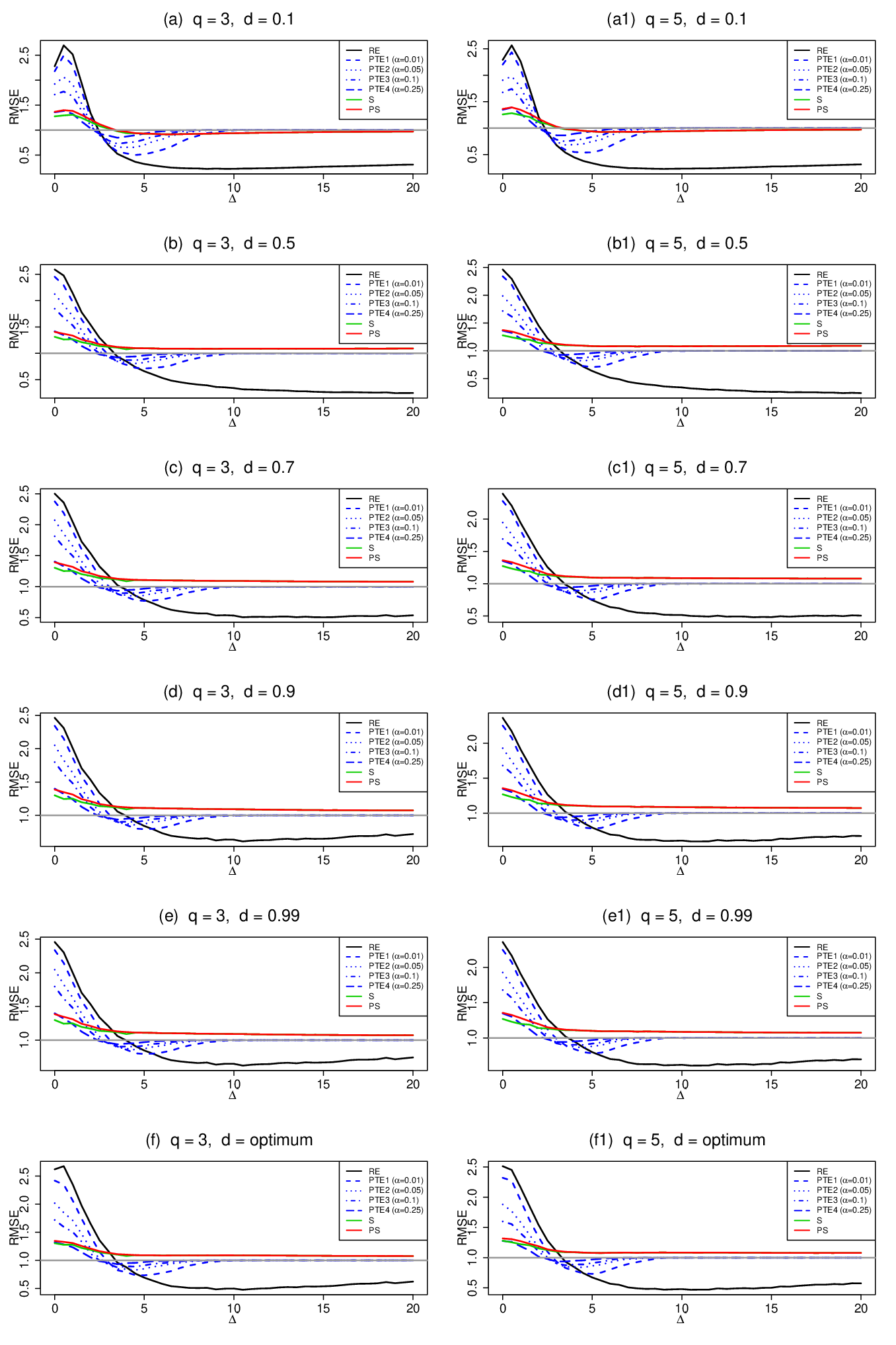
Refer to caption
Figure 1. RMSE

Δ\Delta changes between 00 and 2020. qq is taken to be 33 and 55. The biasing parameter dd is considered to be 0.1,0.5,0.7,0.90.1,0.5,0.7,0.9 and 0.990.99. Following [1] and [31], we also use the following estimator of dd:

(3.1) do​p​t​i​m​u​m=1−(∑j=1p1λj​(λj+1)∑j=1p1+λj​θ^j2λj​(λj+1)4)\displaystyle d_{optimum}=1-\sqrt{\left(\frac{\sum_{j=1}^{p}\frac{1}{\lambda_{j}(\lambda_{j}+1)}}{\sum_{j=1}^{p}\frac{1+\lambda_{j}\widehat{\theta}_{j}^{2}}{\lambda_{j}(\lambda_{j}+1)^{4}}}\right)}

where θ^j\widehat{\theta}_{j} is the jth element of 𝜽^=𝐐⊤​𝜷^MLE\hat{{\bm{\theta}}}={\rm{\mathbf{Q}}}^{\top}\bm{\widehat{\beta}}_{\textrm{MLE}} and 𝐐{\mathbf{Q}} is the orthogonal matrix whose columns consist of eigenvectors of 𝐃{\mathbf{D}}. The simulations are repeated 2000 times. For each replication, we compute the simulated MSE values of each estimator 𝜷∗{\bm{\beta}}^{*} and we obtain the average MSE value using

M​S​E​(𝜷∗)=∑r=12000(𝜷∗−𝜷)r⊤​(𝜷∗−𝜷)r.MSE\left({\bm{\beta}}^{*}\right)=\sum_{r=1}^{2000}\left({\bm{\beta}}^{*}-{\bm{\beta}}\right)_{r}^{\top}\left({\bm{\beta}}^{*}-{\bm{\beta}}\right)_{r}.

We consider the simulated relative mean squared error (RMSE) of each estimator 𝜷∗{\bm{\beta}}^{*} as follows:

R​M​S​E​(𝜷∗)=M​S​E​(𝜷^UR)M​S​E​(𝜷∗)RMSE\left({\bm{\beta}}^{*}\right)=\frac{MSE\left(\bm{\widehat{\beta}}_{\textrm{UR}}\right)}{MSE\left({\bm{\beta}}^{*}\right)}

All the computations are performed using R Statistical Package Program [22]. The results of the simulation is summarized in Figure  1. The findings of Figure  1 can be summarized as follows:

  1. a)

    When the null hypothesis is true, i.e., Δ∗=0\Delta^{\ast}=0, the performance of the RE is the best. On the other hand, the RMSE of the RE slightly decreases and approaches to zero while the null hypothesis is violated. However, it mostly depends on the biasing parameter dd. For example, if d=0.1d=0.1, then the RMSE of the RE interestingly is not the best when Δ∗=0\Delta^{\ast}=0. But, it peaks a small amount violation of the null hypothesis, after that it decreases and approaches to zero. if dd is relative large, say 0.90.9, then the RMSE of the RE may increase while Δ∗\Delta^{\ast} is larger than 10. But, it still remains below to the line one when Δ∗\Delta^{\ast} is enough large.

  2. b)

    We investigate the performance of PTE in four aspects: α=0.01,0.05,0.10,0.25\alpha=0.01,0.05,0.10,0.25. In summary, if α\alpha is smaller, then the PTE performs better when the Δ∗\Delta^{\ast} is between 00 and around 33. For intermediate values of Δ∗\Delta^{\ast}, the RMSE of PTE becomes worser than the UR. Finally, the RMSE of the PTE goes to one when Δ∗\Delta^{\ast} is large.

  3. c)

    It can be shown that the performance of PS outshines the shrinkage estimation for all values of Δ∗\Delta^{\ast}. This is also consistent with our theory. Moreover, the RMSE of PS is only better than PTE with α=0.25\alpha=0.25 when we assume the null hypothesis is true. On the other hand, the RMSE of the PS decreases gradually and approaches to one when the alternative hypothesis is true.

  4. d)

    We also examine that the performance of pretest and shrinkage estimations perform better when the number of ”nuisance parameter” is large.

4. Real Data Application

We consider the heart disease data which was also analyzed by [13] and [12]. There are 462 individuals in this dataset. The dependent variable is an indicator variable showing that whether the individual has a coronary heart disease (chd) or not. The affecting factors are systolic blood pressure (sbp), cumulative tobacco in kg (tobocco), low density lipoprotein cholesterol (ldl), adiposity, family history of heart disease, a factor with levels Absent or Present (famhist), type-A behavior (typea), obesity, current alcohol consumption (alcohol) and age.

Table 1. Cross-validated MSE values of estimators
0.1 0.5 0.7 0.9 0.99 do​p​t​i​m​u​md_{optimum}
UR 120.1662 132.2195 136.0768 138.0744 138.3248 135.6160
RE 114.3332 127.1294 131.2303 133.3549 133.6213 130.7096
PTE1 114.3332 127.1294 131.2303 133.3549 133.6213 130.7096
PTE2 114.3498 127.1451 131.2457 133.3702 133.6365 130.7252
PTE3 114.4550 127.2421 131.3400 133.4631 133.7292 130.8204
PTE4 115.4537 128.1537 132.2234 134.3318 134.5961 131.7128
S 116.7602 129.2675 133.2735 135.3485 135.6087 132.7791
PS 116.7241 129.2121 133.2118 135.2836 135.5434 132.7184

Since there is no prior information, we follow [13] and consider that the candidate subspace is

𝜷2=(sbp, adiposity, obesity, alcohol)=(0,0,0,0).{\bm{\beta}}_{2}=\left(\text{sbp, adiposity, obesity, alcohol}\right)=(0,0,0,0).

We use 10-fold cross-validation and compute the MSE of each estimator and repeat this procedure 500 times. Finally, we compute the average MSE values and report them in Table  1 for different values of the parameter dd. According to Table  1, RE has the best performance which it has the smallest MSE value and PTEs follow it. Shrinkage and its positive perform well compare to the full model estimators. All the shrinkage and preliminary test estimators has lower MSE values than UR which is also satisfied with the results of simulation and theory.

5. Conclusion

This paper introduced the preliminary test almost unbiased Liu, Stein-type shrinkage almost unbiased Liu and positive-rule Stein-type shrinkage almost unbiased Liu estimators in Logistic Regression model, to provide improvement upon the recent approach of [10]. We implemented a sub-space restriction on the parameter 𝜷{\bm{\beta}} to propose improved estimation strategies. Asymptotic distributional bias and quadratic risk of the estimators are exactly given and numerical comparisons provided. We further considered the application of proposed estimators in a real data example. Numerical results confirm that the proposed positive-rule Stein-type shrinkage almost unbiased Liu estimator, which is a derivative of the preliminary one, performs significantly better than all others. Similar conclusions to [25] and [5] are obtained. The availability of these results in this paper should stimulate research and applications.

Appendix

Lemma 5.1.

Let 𝐗{\mathbf{X}} be q−q-dimensional normal vector distributed as N⁡(𝛍x,𝚺q),N\left(\bm{\mu}_{x},\bm{\Sigma}_{q}\right), then, for a measurable function of of φ,\varphi, we have

𝔼⁡[𝐗​φ​(𝐗⊤​𝐗)]=\displaystyle\mathbb{E}\left[{\mathbf{X}}\varphi\left({\mathbf{X}}^{\top}{\mathbf{X}}\right)\right]= 𝝁x​𝔼​[φ​χq+22​(Δ)]\displaystyle\bm{\mu}_{x}\mathbb{E}\left[\varphi\chi_{q+2}^{2}\left(\Delta\right)\right]
𝔼⁡[𝑿​𝑿⊤​φ​(𝐗⊤​𝐗)]=\displaystyle\mathbb{E}\left[\bm{XX}^{\top}\varphi\left({\mathbf{X}}^{\top}{\mathbf{X}}\right)\right]= 𝚺q​𝔼​[φ​χq+22​(Δ)]+𝝁x​𝝁x⊤​𝔼​[φ​χq+42​(Δ)]\displaystyle\bm{\Sigma}_{q}\mathbb{E}\left[\varphi\chi_{q+2}^{2}\left(\Delta\right)\right]+\bm{\mu}_{x}\bm{\mu}_{x}^{\top}\mathbb{E}\left[\varphi\chi_{q+4}^{2}\left(\Delta\right)\right]

where χv2​(Δ)\chi_{v}^{2}\left(\Delta\right) is a non-central chi-square distribution with vv degrees of freedom and non-centrality parameter Δ\Delta.

Proof.

It can be found in [11].  

Proof of Proposition 2.1.

It is easy to obtain the asymptotic bias of UR as follows:

ℬ⁡(𝜷^UR)\displaystyle\mathcal{B}\left(\bm{\widehat{\beta}}_{\textrm{UR}}\right) =\displaystyle= 𝔼⁡{limn→∞​n​(𝜷^UR−𝜷)}\displaystyle\mathbb{E}\left\{\underset{n\rightarrow\infty}{\lim}\sqrt{n}\left(\bm{\widehat{\beta}}_{\textrm{UR}}-{\bm{\beta}}\right)\right\}
=\displaystyle= 𝔼⁡{limn→∞​n​(𝑳d​𝜷^MLE−𝜷)}\displaystyle\mathbb{E}\left\{\underset{n\rightarrow\infty}{\lim}\sqrt{n}\left({\bm{L}_{d}}\bm{\widehat{\beta}}_{\textrm{MLE}}-{\bm{\beta}}\right)\right\}
=\displaystyle= 𝔼⁡{limn→∞​n​[𝐈−(1−d)2​(𝐃+𝐈)−2]​𝜷^MLE−𝜷}\displaystyle\mathbb{E}\left\{\underset{n\rightarrow\infty}{\lim}\sqrt{n}\left[{\mathbf{I}}-(1-d)^{2}\left({\mathbf{D}}+{\mathbf{I}}\right)^{-2}\right]\bm{\widehat{\beta}}_{\textrm{MLE}}-{\bm{\beta}}\right\}
=\displaystyle= 𝔼⁡{limn→∞​n​[(𝜷^MLE−𝜷)−(1−d)2​(𝐃+𝐈)−2]​𝜷^MLE}\displaystyle\mathbb{E}\left\{\underset{n\rightarrow\infty}{\lim}\sqrt{n}\left[\left(\bm{\widehat{\beta}}_{\textrm{MLE}}-{\bm{\beta}}\right)-(1-d)^{2}\left({\mathbf{D}}+{\mathbf{I}}\right)^{-2}\right]\bm{\widehat{\beta}}_{\textrm{MLE}}\right\}
=\displaystyle= −(1−d)2​(𝐃+𝐈)−2​𝜷\displaystyle-(1-d)^{2}\left({\mathbf{D}}+{\mathbf{I}}\right)^{-2}{\bm{\beta}}
=\displaystyle= 𝜻\displaystyle\bm{\zeta}

and also using the definition of asymptotic covariance and making use of Equation (2.12) given in [25], we get the following

(5.1) 𝚪⁡(𝜷^UR)\displaystyle\bm{\Gamma}\left(\bm{\widehat{\beta}}_{\textrm{UR}}\right) =\displaystyle= 𝔼⁡{limn→∞​n​(𝜷^UR−𝜷)​(𝜷^UR−𝜷)⊤}\displaystyle\mathbb{E}\left\{\underset{n\rightarrow\infty}{\lim}{n}\left(\bm{\widehat{\beta}}_{\textrm{UR}}-{\bm{\beta}}\right)\left(\bm{\widehat{\beta}}_{\textrm{UR}}-{\bm{\beta}}\right)^{\top}\right\}
=\displaystyle= 𝔼⁡(ϑ1​ϑ1⊤)\displaystyle\mathbb{E}\left(\bm{\vartheta}_{1}\bm{\vartheta}_{1}^{\top}\right)
=\displaystyle= C​o​v​(ϑ1​ϑ1⊤)+𝔼⁡(ϑ1)​𝔼​(ϑ1⊤)\displaystyle Cov\left(\bm{\vartheta}_{1}\bm{\vartheta}_{1}^{\top}\right)+\mathbb{E}\left(\bm{\vartheta}_{1}\right)\mathbb{E}\left(\bm{\vartheta}_{1}^{\top}\right)
=\displaystyle= 𝑳d​𝐃−1​𝑳d⊤+𝜻​𝜻⊤\displaystyle{\bm{L}_{d}}{\mathbf{D}}^{-1}{\bm{L}_{d}}^{\top}+\bm{\zeta}\bm{\zeta}^{\top}

Thus, ϑ1∼𝒩⁡(𝜻,𝑳d​𝐃−1​𝑳d⊤).\bm{\vartheta}_{1}\sim\mathcal{N}\left(\bm{\zeta},{\bm{L}_{d}}{\mathbf{D}}^{-1}{\bm{L}_{d}}^{\top}\right).
In [25], it is given that the asymptotic distribution of RMLE is 𝜷^RMLE∼𝒩⁡(−𝜹,𝐃−1−𝐀)\bm{\widehat{\beta}}_{\textrm{RMLE}}\sim\mathcal{N}\left(-{\bm{\delta}},{\mathbf{D}}^{-1}-{\mathbf{A}}\right) where 𝐀=𝐃−1​𝐇⊤​(𝐇𝐃−1​𝐇⊤)−1​𝐇𝐃−1{\mathbf{A}}={\mathbf{D}}^{-1}{\mathbf{H}}^{\top}\left({\mathbf{H}}{\mathbf{D}}^{-1}{\mathbf{H}}^{\top}\right)^{-1}{\mathbf{H}}{\mathbf{D}}^{-1} and 𝜹=𝐃−1​𝐇⊤​(𝐇𝐃−1​𝐇⊤)−1​𝜸{\bm{\delta}}={\mathbf{D}}^{-1}{\mathbf{H}}^{\top}\left({\mathbf{H}}{\mathbf{D}}^{-1}{\mathbf{H}}^{\top}\right)^{-1}{\bm{\gamma}}. Thus, similarly, we obtain

ℬ⁡(𝜷^RE)\displaystyle\mathcal{B}\left(\bm{\widehat{\beta}}_{\textrm{RE}}\right) =\displaystyle= 𝔼⁡(ϑ2)\displaystyle\mathbb{E}\left(\bm{\vartheta}_{2}\right)
=\displaystyle= 𝔼⁡{limn→∞​n​(𝜷^RE−𝜷)}\displaystyle\mathbb{E}\left\{\underset{n\rightarrow\infty}{\lim}\sqrt{n}\left(\bm{\widehat{\beta}}_{\textrm{RE}}-{\bm{\beta}}\right)\right\}
=\displaystyle= 𝔼⁡{limn→∞​n​(𝑳d​𝜷^RMLE−𝜷)}\displaystyle\mathbb{E}\left\{\underset{n\rightarrow\infty}{\lim}\sqrt{n}\left({\bm{L}_{d}}\bm{\widehat{\beta}}_{\textrm{RMLE}}-{\bm{\beta}}\right)\right\}
=\displaystyle= 𝔼⁡{limn→∞​n​([𝜷^UR−𝜷]−𝑳d​𝐃−1​𝐇⊤​(𝐇𝐃−1​𝐇⊤)−1​(𝐇​𝜷^MLE−𝐡))}\displaystyle\mathbb{E}\left\{\underset{n\rightarrow\infty}{\lim}\sqrt{n}\left(\left[\bm{\widehat{\beta}}_{\textrm{UR}}-{\bm{\beta}}\right]-{\bm{L}_{d}}{\mathbf{D}}^{-1}{\mathbf{H}}^{\top}\left({\mathbf{H}}{\mathbf{D}}^{-1}{\mathbf{H}}^{\top}\right)^{-1}\left({\mathbf{H}}\bm{\widehat{\beta}}_{\textrm{MLE}}-{\mathbf{h}}\right)\right)\right\}
=\displaystyle= 𝜻−𝑳d​𝜹.\displaystyle\bm{\zeta}-{\bm{L}_{d}}{\bm{\delta}}.

Now, we need to compute 𝚪⁡(𝜷^RE){\bm{\Gamma}}\left(\bm{\widehat{\beta}}_{\textrm{RE}}\right) which is as follows:

(5.2) 𝚪⁡(𝜷^RE)\displaystyle{\bm{\Gamma}}\left(\bm{\widehat{\beta}}_{\textrm{RE}}\right) =\displaystyle= 𝔼⁡{limn→∞​n​(𝜷^RE−𝜷)​(𝜷^RE−𝜷)⊤}\displaystyle\mathbb{E}\left\{\underset{n\rightarrow\infty}{\lim}{n}\left(\bm{\widehat{\beta}}_{\textrm{RE}}-{\bm{\beta}}\right)\left(\bm{\widehat{\beta}}_{\textrm{RE}}-{\bm{\beta}}\right)^{\top}\right\}
=\displaystyle= 𝔼⁡(ϑ2​ϑ2⊤)\displaystyle\mathbb{E}\left(\bm{\vartheta}_{2}\bm{\vartheta}_{2}^{\top}\right)
=\displaystyle= 𝑪​𝒐​𝒗​(ϑ2​ϑ2⊤)+𝔼⁡(ϑ2)​𝔼​(ϑ2⊤)\displaystyle\bm{Cov}\left(\bm{\vartheta}_{2}\bm{\vartheta}_{2}^{\top}\right)+\mathbb{E}\left(\bm{\vartheta}_{2}\right)\mathbb{E}\left(\bm{\vartheta}_{2}^{\top}\right)
=\displaystyle= 𝑳d​(𝐃−1−𝐀)​𝑳d⊤+(𝜻−𝑳d​𝜹)​(𝜻−𝑳d​𝜹)⊤\displaystyle{\bm{L}_{d}}\left({\mathbf{D}}^{-1}-{\mathbf{A}}\right){\bm{L}_{d}}^{\top}+\left(\bm{\zeta}-{\bm{L}_{d}}{\bm{\delta}}\right)\left(\bm{\zeta}-{\bm{L}_{d}}{\bm{\delta}}\right)^{\top}
=\displaystyle= 𝑳d​(𝐃−1−𝐀)​𝑳d⊤+[(1−d)2​(𝐃+𝐈)−2​𝜷+𝐋d​𝜹]​[(1−d)2​(𝐃+𝐈)−2​𝜷+𝐋d​𝜹]⊤\displaystyle{\bm{L}_{d}}\left({\mathbf{D}}^{-1}-{\mathbf{A}}\right){\bm{L}_{d}}^{\top}+\left[\left(1-d\right)^{2}\left({\mathbf{D}}+{\mathbf{I}}\right)^{-2}{\bm{\beta}}+{\mathbf{L}}_{d}{\bm{\delta}}\right]\left[\left(1-d\right)^{2}\left({\mathbf{D}}+{\mathbf{I}}\right)^{-2}{\bm{\beta}}+{\mathbf{L}}_{d}{\bm{\delta}}\right]^{\top}
=\displaystyle= 𝑳d​(𝐃−1−𝐀)​𝑳d⊤+(1−d)2​(𝐃+𝐈)−2​𝜷​𝜹⊤​𝐋d⊤+(1−d)2​𝐋d​𝜹​𝜷⊤​(𝐃+𝐈)−2\displaystyle{\bm{L}_{d}}\left({\mathbf{D}}^{-1}-{\mathbf{A}}\right){\bm{L}_{d}}^{\top}+\left(1-d\right)^{2}\left({\mathbf{D}}+{\mathbf{I}}\right)^{-2}{\bm{\beta}}{\bm{\delta}}^{\top}{\mathbf{L}}_{d}^{\top}+\left(1-d\right)^{2}{\mathbf{L}}_{d}{\bm{\delta}}{\bm{\beta}}^{\top}\left({\mathbf{D}}+{\mathbf{I}}\right)^{-2}
+𝐋d​𝜹​𝜹⊤​𝐋d⊤+(1−d)4​(𝐃+𝐈)−2​𝜷​𝜷⊤​(𝐃+𝐈)−2\displaystyle+{\mathbf{L}}_{d}{\bm{\delta}}{\bm{\delta}}^{\top}{\mathbf{L}}_{d}^{\top}+\left(1-d\right)^{4}\left({\mathbf{D}}+{\mathbf{I}}\right)^{-2}{\bm{\beta}}{\bm{\beta}}^{\top}\left({\mathbf{D}}+{\mathbf{I}}\right)^{-2}

Thus, ϑ2∼𝒩⁡(𝜻−𝑳d​𝜹,𝑳d​(𝐃−1−A)​𝑳d⊤)\bm{\vartheta}_{2}\sim\mathcal{N}\left(\bm{\zeta}-{\bm{L}_{d}}{\bm{\delta}},{\bm{L}_{d}}\left({\mathbf{D}}^{-1}-A\right){\bm{L}_{d}}^{\top}\right).

Moreover, to obtain the asymptotic distribution of ϑ3\bm{\vartheta}_{3}, we start with the following:

𝔼⁡(ϑ3)\displaystyle\mathbb{E}\left(\bm{\vartheta}_{3}\right) =\displaystyle= 𝔼⁡{limn→∞​n​(𝜷^UR−𝜷^RE)}\displaystyle\mathbb{E}\left\{\underset{n\rightarrow\infty}{\lim}\sqrt{n}\left(\bm{\widehat{\beta}}_{\textrm{UR}}-\bm{\widehat{\beta}}_{\textrm{RE}}\right)\right\}
=\displaystyle= 𝔼⁡{limn→∞​n​𝑳d​(𝐃−1​𝐇⊤​(𝐇𝐃−1​𝐇⊤)−1​(𝐇​𝜷^MLE−𝐡))}\displaystyle\mathbb{E}\left\{\underset{n\rightarrow\infty}{\lim}\sqrt{n}{\bm{L}_{d}}\left({\mathbf{D}}^{-1}{\mathbf{H}}^{\top}\left({\mathbf{H}}{\mathbf{D}}^{-1}{\mathbf{H}}^{\top}\right)^{-1}\left({\mathbf{H}}\bm{\widehat{\beta}}_{\textrm{MLE}}-{\mathbf{h}}\right)\right)\right\}
=\displaystyle= 𝑳d​𝜹\displaystyle{\bm{L}_{d}}{\bm{\delta}}

and to compute the covariance matrix of ϑ3\vartheta_{3} we compute as follows:

C​o​v​(ϑ3,ϑ3⊤)\displaystyle Cov\left(\bm{\vartheta}_{3},\bm{\vartheta}_{3}^{\top}\right) =\displaystyle= C​o​v​(𝜷^UR−𝜷^RE)\displaystyle Cov\left(\bm{\widehat{\beta}}_{\textrm{UR}}-\bm{\widehat{\beta}}_{\textrm{RE}}\right)
=\displaystyle= C​o​v​(𝑳d​(𝜷^MLE−𝜷^RMLE))\displaystyle Cov\left({\bm{L}_{d}}\left(\bm{\widehat{\beta}}_{\textrm{MLE}}-\bm{\widehat{\beta}}_{\textrm{RMLE}}\right)\right)
=\displaystyle= 𝑳d​𝐀​𝑳d⊤\displaystyle{\bm{L}_{d}}{\mathbf{A}}{\bm{L}_{d}}^{\top}

Thus, ϑ3∼𝒩⁡(𝑳d​𝜹,𝑳d​𝐀​𝑳d⊤)\bm{\vartheta}_{3}\sim{\mathcal{N}\left({\bm{L}_{d}}{\bm{\delta}},{\bm{L}_{d}}{\mathbf{A}}{\bm{L}_{d}}^{\top}\right)}.

Now, we also need to compute C​o​v​(ϑ1,ϑ3)Cov\left(\bm{\vartheta}_{1},\bm{\vartheta}_{3}\right) and C​o​v​(ϑ2,ϑ3)Cov\left(\bm{\vartheta}_{2},\bm{\vartheta}_{3}\right). We start with computing C​o​v​(ϑ1,ϑ3)Cov\left(\bm{\vartheta}_{1},\bm{\vartheta}_{3}\right) as follows:

C​o​v​(ϑ1,ϑ3)\displaystyle Cov\left(\bm{\vartheta}_{1},\bm{\vartheta}_{3}\right) =\displaystyle= C​o​v​(𝜷^UR,𝜷^UR−𝜷^RE)\displaystyle Cov\left(\bm{\widehat{\beta}}_{\textrm{UR}},\bm{\widehat{\beta}}_{\textrm{UR}}-\bm{\widehat{\beta}}_{\textrm{RE}}\right)
=\displaystyle= C​o​v​(𝜷^UR,𝜷^UR)−C​o​v​(𝜷^UR,𝜷^RE)\displaystyle Cov\left(\bm{\widehat{\beta}}_{\textrm{UR}},\bm{\widehat{\beta}}_{\textrm{UR}}\right)-Cov\left(\bm{\widehat{\beta}}_{\textrm{UR}},\bm{\widehat{\beta}}_{\textrm{RE}}\right)
=\displaystyle= 𝑳d​𝐃−1​𝑳d⊤−C​o​v​(𝑳d​𝜷^MLE,𝑳d​𝜷^RMLE)\displaystyle{\bm{L}_{d}}{\mathbf{D}}^{-1}{\bm{L}_{d}}^{\top}-Cov\left({\bm{L}_{d}}\bm{\widehat{\beta}}_{\textrm{MLE}},{\bm{L}_{d}}\bm{\widehat{\beta}}_{\textrm{RMLE}}\right)
=\displaystyle= 𝑳d​𝐃−1​𝑳d⊤−𝑳d​C​o​v​(𝜷^MLE,𝜷^RMLE)​𝑳d⊤\displaystyle{\bm{L}_{d}}{\mathbf{D}}^{-1}{\bm{L}_{d}}^{\top}-{\bm{L}_{d}}Cov\left(\bm{\widehat{\beta}}_{\textrm{MLE}},\bm{\widehat{\beta}}_{\textrm{RMLE}}\right){\bm{L}_{d}}^{\top}
=\displaystyle= 𝑳d​𝐃−1​𝑳d⊤−𝑳d​(𝐃−1−𝐀)​𝑳d⊤\displaystyle{\bm{L}_{d}}{\mathbf{D}}^{-1}{\bm{L}_{d}}^{\top}-{\bm{L}_{d}}\left({\mathbf{D}}^{-1}-{\mathbf{A}}\right){\bm{L}_{d}}^{\top}
=\displaystyle= 𝑳d​𝐀​𝑳d⊤\displaystyle{\bm{L}_{d}}{\mathbf{A}}{\bm{L}_{d}}^{\top}

Finally, C​o​v​(ϑ2,ϑ3)Cov\left(\bm{\vartheta}_{2},\bm{\vartheta}_{3}\right) is obtained as follows: C​o​v​(ϑ2,ϑ3)Cov\left(\bm{\vartheta}_{2},\bm{\vartheta}_{3}\right) is obtained as follows:

C​o​v​(ϑ2,ϑ3)\displaystyle Cov\left(\bm{\vartheta}_{2},\bm{\vartheta}_{3}\right) =\displaystyle= C​o​v​(𝜷^RE,𝜷^UR−𝜷^RE)\displaystyle Cov\left(\bm{\widehat{\beta}}_{\textrm{RE}},\bm{\widehat{\beta}}_{\textrm{UR}}-\bm{\widehat{\beta}}_{\textrm{RE}}\right)
=\displaystyle= C​o​v​(𝜷^RE,𝜷^UR)−C​o​v​(𝜷^RE,𝜷^RE)\displaystyle Cov\left(\bm{\widehat{\beta}}_{\textrm{RE}},\bm{\widehat{\beta}}_{\textrm{UR}}\right)-Cov\left(\bm{\widehat{\beta}}_{\textrm{RE}},\bm{\widehat{\beta}}_{\textrm{RE}}\right)
=\displaystyle= 𝑳d​(𝐃−1−𝐀)​𝑳d⊤−𝑳d​(𝐃−1−𝐀)​𝑳d⊤\displaystyle{\bm{L}_{d}}\left({\mathbf{D}}^{-1}-{\mathbf{A}}\right){\bm{L}_{d}}^{\top}-{\bm{L}_{d}}\left({\mathbf{D}}^{-1}-{\mathbf{A}}\right){\bm{L}_{d}}^{\top}
=\displaystyle= 𝟎p+1\displaystyle{\mathbf{0}}_{p+1}

The proof is finished.  

Proof of Theorem 2.2.

The asymptotic biases of UR ans RE are already obtained in the proof of Proposition 2.1. Now, we continue computing the asymptotic bias of PT as follows:

ℬ⁡(𝜷^PT)\displaystyle\mathcal{B}\left(\bm{\widehat{\beta}}_{\textrm{PT}}\right) =\displaystyle= 𝔼⁡{limn→∞​n​(𝜷^PT−𝜷)}\displaystyle\mathbb{E}\left\{\underset{n\rightarrow\infty}{\lim}\sqrt{n}\left(\bm{\widehat{\beta}}_{\textrm{PT}}-{\bm{\beta}}\right)\right\}
=\displaystyle= 𝔼{limn→∞n(𝜷^UR−(𝜷^UR−𝜷^RE)I[Ln<χq,α2]−𝜷)}\displaystyle\mathbb{E}\left\{\underset{n\rightarrow\infty}{\lim}\sqrt{n}\left(\bm{\widehat{\beta}}_{\textrm{UR}}-\left(\bm{\widehat{\beta}}_{\textrm{UR}}-\bm{\widehat{\beta}}_{\textrm{RE}}\right)\textrm{I}\left[L_{n}<\chi_{q,\alpha}^{2}\right]-{\bm{\beta}}\right)\right\}
=\displaystyle= 𝔼{limn→∞n(𝜷^UR−𝜷−(𝜷^UR−𝜷^RE)I[Ln<χq,α2])}\displaystyle\mathbb{E}\left\{\underset{n\rightarrow\infty}{\lim}\sqrt{n}\left(\bm{\widehat{\beta}}_{\textrm{UR}}-{\bm{\beta}}-\left(\bm{\widehat{\beta}}_{\textrm{UR}}-\bm{\widehat{\beta}}_{\textrm{RE}}\right)\textrm{I}\left[L_{n}<\chi_{q,\alpha}^{2}\right]\right)\right\}
=\displaystyle= 𝜻−𝑳d​𝜹​ℍq+2​(χq,α2,Δ2)\displaystyle\bm{\zeta}-{\bm{L}_{d}}{\bm{\delta}}\mathbb{H}_{q+2}\left(\chi_{q,\alpha}^{2};\Delta^{2}\right)
ℬ⁡(𝜷^S)\displaystyle\mathcal{B}\left(\bm{\widehat{\beta}}_{\textrm{S}}\right) =\displaystyle= 𝔼⁡{limn→∞​n​(𝜷^S−𝜷)}\displaystyle\mathbb{E}\left\{\underset{n\rightarrow\infty}{\lim}\sqrt{n}\left(\bm{\widehat{\beta}}_{\textrm{S}}-{\bm{\beta}}\right)\right\}
=\displaystyle= 𝔼⁡{limn→∞​n​(𝜷^UR−(𝜷^UR−𝜷^RE)​c​Ln−1−𝜷)}\displaystyle\mathbb{E}\left\{\underset{n\rightarrow\infty}{\lim}\sqrt{n}\left(\bm{\widehat{\beta}}_{\textrm{UR}}-\left(\bm{\widehat{\beta}}_{\textrm{UR}}-\bm{\widehat{\beta}}_{\textrm{RE}}\right)cL_{n}^{-1}-{\bm{\beta}}\right)\right\}
=\displaystyle= 𝔼⁡{limn→∞​n​(𝜷^UR−𝜷)}−𝔼⁡{limn→∞​n​(𝜷^UR−𝜷^RE)​c​Ln−1}\displaystyle\mathbb{E}\left\{\underset{n\rightarrow\infty}{\lim}\sqrt{n}\left(\bm{\widehat{\beta}}_{\textrm{UR}}-{\bm{\beta}}\right)\right\}-\mathbb{E}\left\{\underset{n\rightarrow\infty}{\lim}\sqrt{n}\left(\bm{\widehat{\beta}}_{\textrm{UR}}-\bm{\widehat{\beta}}_{\textrm{RE}}\right)cL_{n}^{-1}\right\}
=\displaystyle= 𝜻−c​𝑳d​𝜹​𝔼​(χq+2−2​(Δ2))\displaystyle\bm{\zeta}-c{\bm{L}_{d}}{\bm{\delta}}\mathbb{E}\left(\chi_{q+2}^{-2}(\Delta^{2})\right)
ℬ⁡(𝜷^PS)\displaystyle\mathcal{B}\left(\bm{\widehat{\beta}}_{\textrm{PS}}\right) =\displaystyle= 𝔼⁡{limn→∞​n​(𝜷^S−𝜷)}\displaystyle\mathbb{E}\left\{\underset{n\rightarrow\infty}{\lim}\sqrt{n}\left(\bm{\widehat{\beta}}_{\textrm{S}}-{\bm{\beta}}\right)\right\}
=\displaystyle= 𝔼⁡{limn→∞​n​(𝜷^S−(𝜷^UR−𝜷^RE)​(1−c​Ln−1)​I​(Ln≤c)−𝜷)}\displaystyle\mathbb{E}\left\{\underset{n\rightarrow\infty}{\lim}\sqrt{n}\left(\bm{\widehat{\beta}}_{\textrm{S}}-\left(\bm{\widehat{\beta}}_{\textrm{UR}}-\bm{\widehat{\beta}}_{\textrm{RE}}\right)\left(1-cL_{n}^{-1}\right)\textrm{I}\left(L_{n}\leq c\right)-{\bm{\beta}}\right)\right\}
=\displaystyle= 𝔼⁡{limn→∞​n​(𝜷^S−𝜷)}−𝔼⁡{limn→∞​n​(𝜷^UR−𝜷^RE)​I​(Ln≤c)}\displaystyle\mathbb{E}\left\{\underset{n\rightarrow\infty}{\lim}\sqrt{n}\left(\bm{\widehat{\beta}}_{\textrm{S}}-{\bm{\beta}}\right)\right\}-\mathbb{E}\left\{\underset{n\rightarrow\infty}{\lim}\sqrt{n}\left(\bm{\widehat{\beta}}_{\textrm{UR}}-\bm{\widehat{\beta}}_{\textrm{RE}}\right)\textrm{I}(L_{n}\leq c)\right\}
+𝔼⁡{limn→∞​n​(𝜷^UR−𝜷^RE)​c​Ln−1​I​(Ln<c)}\displaystyle+\mathbb{E}\left\{\underset{n\rightarrow\infty}{\lim}\sqrt{n}\left(\bm{\widehat{\beta}}_{\textrm{UR}}-\bm{\widehat{\beta}}_{\textrm{RE}}\right)cL_{n}^{-1}\textrm{I}(L_{n}<c)\right\}
=\displaystyle= 𝜻−𝑳d​𝜹​𝔼​(χq+2−2​(Δ2))−𝑳d​𝜹​ℍq+2​(χq,α2,Δ2)\displaystyle\bm{\zeta}-{\bm{L}_{d}}{\bm{\delta}}\mathbb{E}\left(\chi_{q+2}^{-2}(\Delta^{2})\right)-{\bm{L}_{d}}{\bm{\delta}}\mathbb{H}_{q+2}\left(\chi_{q,\alpha}^{2};\Delta^{2}\right)
+c​𝑳d​𝜹​𝔼​(χq+2−2​(Δ2)​I​(χq+22​(Δ2)<c))\displaystyle+c{\bm{L}_{d}}{\bm{\delta}}\mathbb{E}\left(\chi_{q+2}^{-2}(\Delta^{2})\textrm{I}\left(\chi_{q+2}^{2}(\Delta^{2})<c\right)\right)


Proof of Theorem  2.4.

The asymptotic covariance of 𝜷^UR\bm{\widehat{\beta}}_{\textrm{UR}} and 𝜷^RE\bm{\widehat{\beta}}_{\textrm{RE}} are already obtained in the proof of Theorem 2.1 respectively in Eqns.  5.1 and  5.2. Now, we continue with the covariance of 𝜷^PT\bm{\widehat{\beta}}_{\textrm{PT}} as follows:

𝚪⁡(𝜷^PT)\displaystyle{\bm{\Gamma}}\left(\bm{\widehat{\beta}}_{\textrm{PT}}\right) =\displaystyle= 𝔼⁡{limn→∞​n​(𝜷^PT−𝜷)​(𝜷^PT−𝜷)⊤}\displaystyle\mathbb{E}\left\{\underset{n\rightarrow\infty}{\lim}\sqrt{n}\left(\bm{\widehat{\beta}}_{\textrm{PT}}-{\bm{\beta}}\right)\left(\bm{\widehat{\beta}}_{\textrm{PT}}-{\bm{\beta}}\right)^{\top}\right\}
=\displaystyle= 𝔼{limn→∞n[(𝜷^UR−𝜷)−(𝜷^UR−𝜷^RE)I(Ln<χq,α2)]\displaystyle\mathbb{E}\left\{\underset{n\rightarrow\infty}{\lim}\sqrt{n}\left[\left(\bm{\widehat{\beta}}_{\textrm{UR}}-{\bm{\beta}}\right)-\left(\bm{\widehat{\beta}}_{\textrm{UR}}-\bm{\widehat{\beta}}_{\textrm{RE}}\right)\textrm{I}\left(L_{n}<\chi_{q,\alpha}^{2}\right)\right]\right.
×[(𝜷^UR−𝜷)−(𝜷^UR−𝜷^RE)I(Ln<χq,α2)]⊤}\displaystyle\left.\times\left[\left(\bm{\widehat{\beta}}_{\textrm{UR}}-{\bm{\beta}}\right)-\left(\bm{\widehat{\beta}}_{\textrm{UR}}-\bm{\widehat{\beta}}_{\textrm{RE}}\right)\textrm{I}\left(L_{n}<\chi_{q,\alpha}^{2}\right)\right]^{\top}\right\}
=\displaystyle= 𝔼⁡{ϑ1​ϑ1⊤−2​ϑ3​ϑ1⊤​I​(Ln<χq,α2)+ϑ3​ϑ3⊤​I​(Ln<χq,α2)}.\displaystyle{\mathbb{E}}\left\{\bm{\vartheta}_{1}\bm{\vartheta}_{1}^{\top}-2\bm{\vartheta}_{3}\bm{\vartheta}_{1}^{\top}\textrm{I}\left(L_{n}<\chi_{q,\alpha}^{2}\right)+\bm{\vartheta}_{3}\bm{\vartheta}_{3}^{\top}\textrm{I}\left(L_{n}<\chi_{q,\alpha}^{2}\right)\right\}.

We already have 𝔼⁡{ϑ1​ϑ1⊤}=𝑳d​𝐃−1​𝑳d⊤+𝜻​𝜻⊤{\mathbb{E}}\left\{\bm{\vartheta}_{1}\bm{\vartheta}_{1}^{\top}\right\}={\bm{L}_{d}}{\mathbf{D}}^{-1}{\bm{L}_{d}}^{\top}+\bm{\zeta}\bm{\zeta}^{\top}. We need the followings:

𝔼⁡{ϑ3​ϑ3⊤​I​(Ln<χq,α2)}=𝑳d​𝐀​𝑳d⊤​ℍq+2​(χq,α2,Δ2)+𝑳d​𝜹​𝜹⊤​𝑳d⊤​ℍq+4​(χq,α2,Δ2)\displaystyle{\mathbb{E}}\left\{\bm{\vartheta}_{3}\bm{\vartheta}_{3}^{\top}\textrm{I}\left(L_{n}<\chi_{q,\alpha}^{2}\right)\right\}={\bm{L}_{d}}{\mathbf{A}}{\bm{L}_{d}}^{\top}{\mathbb{H}}_{q+2}\left(\chi_{q,\alpha}^{2};\Delta^{2}\right)+{\bm{L}_{d}}{\bm{\delta}}{\bm{\delta}}^{\top}{\bm{L}_{d}}^{\top}{\mathbb{H}}_{q+4}\left(\chi_{q,\alpha}^{2};\Delta^{2}\right)

and

𝔼⁡{ϑ3​ϑ1⊤​I​(Ln<χq,α2)}\displaystyle{\mathbb{E}}\left\{\bm{\vartheta}_{3}\bm{\vartheta}_{1}^{\top}\textrm{I}\left(L_{n}<\chi_{q,\alpha}^{2}\right)\right\} =\displaystyle= 𝔼⁡{ϑ3​𝔼​[ϑ1⊤​I​(Ln<χq,α2)|ϑ3]}\displaystyle{\mathbb{E}}\left\{\bm{\vartheta}_{3}{\mathbb{E}}\left[\bm{\vartheta}_{1}^{\top}\textrm{I}\left(L_{n}<\chi_{q,\alpha}^{2}\right)|\bm{\vartheta}_{3}\right]\right\}
=\displaystyle= 𝔼⁡{ϑ3​[𝜻+ϑ3−𝐋d​𝜹]⊤​I​(Ln<χq,α2)}\displaystyle{\mathbb{E}}\left\{\bm{\vartheta}_{3}\left[\bm{\zeta}+\bm{\vartheta}_{3}-{\mathbf{L}}_{d}{\bm{\delta}}\right]^{\top}\textrm{I}\left(L_{n}<\chi_{q,\alpha}^{2}\right)\right\}
=\displaystyle= 𝔼⁡{(ϑ3​𝜻⊤+ϑ3​ϑ3⊤−ϑ3​𝜹⊤​𝐋d⊤)​I​(Ln<χq,α2)}\displaystyle{\mathbb{E}}\left\{\left(\bm{\vartheta}_{3}\bm{\zeta}^{\top}+\bm{\vartheta}_{3}\bm{\vartheta}_{3}^{\top}-\bm{\vartheta}_{3}{\bm{\delta}}^{\top}{\mathbf{L}}_{d}^{\top}\right)\textrm{I}\left(L_{n}<\chi_{q,\alpha}^{2}\right)\right\}
=\displaystyle= (𝐋d​𝜹​𝜻⊤+𝐋d​𝐀𝐋d⊤−𝐋d​𝜹​𝜹⊤​𝐋d⊤)​ℍq+2​(χq,α2,Δ2)+𝐋d​𝜹​𝜹⊤​𝐋d⊤​ℍq+4​(χq,α2,Δ2)\displaystyle\left({\mathbf{L}}_{d}{\bm{\delta}}\bm{\zeta}^{\top}+{\mathbf{L}}_{d}{\mathbf{A}}{\mathbf{L}}_{d}^{\top}-{\mathbf{L}}_{d}{\bm{\delta}}{\bm{\delta}}^{\top}{\mathbf{L}}_{d}^{\top}\right){\mathbb{H}}_{q+2}\left(\chi_{q,\alpha}^{2};\Delta^{2}\right)+{\mathbf{L}}_{d}{\bm{\delta}}{\bm{\delta}}^{\top}{\mathbf{L}}_{d}^{\top}{\mathbb{H}}_{q+4}\left(\chi_{q,\alpha}^{2};\Delta^{2}\right)

Thus, we obtain

(5.3) 𝚪⁡(𝜷^PT)\displaystyle{\bm{\Gamma}}\left(\bm{\widehat{\beta}}_{\textrm{PT}}\right) =\displaystyle= 𝑳d​𝐃−1​𝑳d⊤+𝜻​𝜻⊤−𝐋d​𝐀𝐋d⊤​ℍq+2​(χq,α2,Δ2)−2​𝐋d​𝜹​𝜻⊤​ℍq+2​(χq,α2,Δ2)\displaystyle{\bm{L}_{d}}{\mathbf{D}}^{-1}{\bm{L}_{d}}^{\top}+\bm{\zeta}\bm{\zeta}^{\top}-{\mathbf{L}}_{d}{\mathbf{A}}{\mathbf{L}}_{d}^{\top}{\mathbb{H}}_{q+2}\left(\chi_{q,\alpha}^{2};\Delta^{2}\right)-2{\mathbf{L}}_{d}{\bm{\delta}}\bm{\zeta}^{\top}{\mathbb{H}}_{q+2}\left(\chi_{q,\alpha}^{2};\Delta^{2}\right)
+𝐋d​𝜹​𝜹⊤​𝐋d⊤​[2​ℍq+2​(χq,α2,Δ2)−ℍq+4​(χq+42,Δ2)].\displaystyle+{\mathbf{L}}_{d}{\bm{\delta}}{\bm{\delta}}^{\top}{\mathbf{L}}_{d}^{\top}\left[2{\mathbb{H}}_{q+2}\left(\chi_{q,\alpha}^{2};\Delta^{2}\right)-{\mathbb{H}}_{q+4}\left(\chi_{q+4}^{2};\Delta^{2}\right)\right].

In a similar manner, the asymptotic covariance of 𝜷^S\bm{\widehat{\beta}}_{\textrm{S}} can be obtained as follows:

𝚪⁡(𝜷^S)\displaystyle{\bm{\Gamma}}\left(\bm{\widehat{\beta}}_{\textrm{S}}\right) =\displaystyle= 𝔼⁡{limn→∞​n​(𝜷^S−𝜷)​(𝜷^S−𝜷)⊤}\displaystyle\mathbb{E}\left\{\underset{n\rightarrow\infty}{\lim}\sqrt{n}\left(\bm{\widehat{\beta}}_{\textrm{S}}-{\bm{\beta}}\right)\left(\bm{\widehat{\beta}}_{\textrm{S}}-{\bm{\beta}}\right)^{\top}\right\}
=\displaystyle= 𝔼{limn→∞n[(𝜷^UR−𝜷)−c(𝜷^UR−𝜷^RE)Ln−1]\displaystyle\mathbb{E}\left\{\underset{n\rightarrow\infty}{\lim}\sqrt{n}\left[\left(\bm{\widehat{\beta}}_{\textrm{UR}}-{\bm{\beta}}\right)-c\left(\bm{\widehat{\beta}}_{\textrm{UR}}-\bm{\widehat{\beta}}_{\textrm{RE}}\right)L_{n}^{-1}\right]\right.
×[(𝜷^UR−𝜷)−c(𝜷^UR−𝜷^RE)Ln−1]⊤}\displaystyle\left.\times\left[\left(\bm{\widehat{\beta}}_{\textrm{UR}}-{\bm{\beta}}\right)-c\left(\bm{\widehat{\beta}}_{\textrm{UR}}-\bm{\widehat{\beta}}_{\textrm{RE}}\right)L_{n}^{-1}\right]^{\top}\right\}
=\displaystyle= 𝔼⁡{ϑ1​ϑ1⊤−2​c​ϑ3​ϑ1⊤​Ln−1+c2​ϑ3​ϑ3⊤​Ln−2}.\displaystyle{\mathbb{E}}\left\{\bm{\vartheta}_{1}\bm{\vartheta}_{1}^{\top}-2c\bm{\vartheta}_{3}\bm{\vartheta}_{1}^{\top}L_{n}^{-1}+c^{2}\bm{\vartheta}_{3}\bm{\vartheta}_{3}^{\top}L_{n}^{-2}\right\}.

Thus, we need the following identities:

𝔼⁡{ϑ3​ϑ3⊤​Ln−2}=𝑳d​𝐀​𝑳d⊤​𝔼​(χq+2−4​(Δ2))+𝑳d​𝜹​𝜹⊤​𝑳d⊤​𝔼​(χq+4−4​(Δ2))\displaystyle{\mathbb{E}}\left\{\bm{\vartheta}_{3}\bm{\vartheta}_{3}^{\top}L_{n}^{-2}\right\}={\bm{L}_{d}}{\mathbf{A}}{\bm{L}_{d}}^{\top}{\mathbb{E}}\left(\chi_{q+2}^{-4}\left(\Delta^{2}\right)\right)+{\bm{L}_{d}}{\bm{\delta}}{\bm{\delta}}^{\top}{\bm{L}_{d}}^{\top}{\mathbb{E}}\left(\chi_{q+4}^{-4}\left(\Delta^{2}\right)\right)

and

𝔼⁡{ϑ3​ϑ1⊤​Ln−1}\displaystyle{\mathbb{E}}\left\{\bm{\vartheta}_{3}\bm{\vartheta}_{1}^{\top}L_{n}^{-1}\right\} =\displaystyle= 𝔼⁡{ϑ3​𝔼​[ϑ1⊤​Ln−1|ϑ3]}\displaystyle{\mathbb{E}}\left\{\bm{\vartheta}_{3}{\mathbb{E}}\left[\bm{\vartheta}_{1}^{\top}L_{n}^{-1}|\bm{\vartheta}_{3}\right]\right\}
=\displaystyle= 𝔼⁡{ϑ3​[𝜻+ϑ3−𝐋d​𝜹]⊤​Ln−1}\displaystyle{\mathbb{E}}\left\{\bm{\vartheta}_{3}\left[\bm{\zeta}+\bm{\vartheta}_{3}-{\mathbf{L}}_{d}{\bm{\delta}}\right]^{\top}L_{n}^{-1}\right\}
=\displaystyle= 𝔼⁡{ϑ3​𝜻⊤​Ln−1+ϑ3​ϑ3⊤​Ln−1−ϑ3​𝜹⊤​𝐋d⊤​Ln−1}\displaystyle{\mathbb{E}}\left\{\bm{\vartheta}_{3}\bm{\zeta}^{\top}L_{n}^{-1}+\bm{\vartheta}_{3}\bm{\vartheta}_{3}^{\top}L_{n}^{-1}-\bm{\vartheta}_{3}{\bm{\delta}}^{\top}{\mathbf{L}}_{d}^{\top}L_{n}^{-1}\right\}
=\displaystyle= 𝔼⁡(χq+2−2​(Δ2))​(𝐋d​𝜹​𝜻⊤+𝐋d​𝐀𝐋d⊤−𝐋d​𝜹​𝜹⊤​𝐋d⊤)+𝔼⁡(χq+4−2​(Δ2))​𝐋d​𝜹​𝜹⊤​𝐋d⊤.\displaystyle{\mathbb{E}}\left(\chi_{q+2}^{-2}\left(\Delta^{2}\right)\right)\left({\mathbf{L}}_{d}{\bm{\delta}}\bm{\zeta}^{\top}+{\mathbf{L}}_{d}{\mathbf{A}}{\mathbf{L}}_{d}^{\top}-{\mathbf{L}}_{d}{\bm{\delta}}{\bm{\delta}}^{\top}{\mathbf{L}}_{d}^{\top}\right)+{\mathbb{E}}\left(\chi_{q+4}^{-2}\left(\Delta^{2}\right)\right){\mathbf{L}}_{d}{\bm{\delta}}{\bm{\delta}}^{\top}{\mathbf{L}}_{d}^{\top}.

Therefore, we obtain

(5.4) 𝚪⁡(𝜷^S)\displaystyle{\bm{\Gamma}}\left(\bm{\widehat{\beta}}_{\textrm{S}}\right) =\displaystyle= 𝑳d​𝐃−1​𝑳d⊤+𝜻​𝜻⊤−𝐋d​𝐀𝐋d⊤​(c2​𝔼​{χq+2−4​(Δ2)}−2​c​𝔼​{χq+2−2​(Δ2)})\displaystyle{\bm{L}_{d}}{\mathbf{D}}^{-1}{\bm{L}_{d}}^{\top}+\bm{\zeta}\bm{\zeta}^{\top}-{\mathbf{L}}_{d}{\mathbf{A}}{\mathbf{L}}_{d}^{\top}\left(c^{2}{\mathbb{E}}\left\{\chi_{q+2}^{-4}\left(\Delta^{2}\right)\right\}-2c{\mathbb{E}}\left\{\chi_{q+2}^{-2}\left(\Delta^{2}\right)\right\}\right)
+𝐋d​𝜹​𝜹⊤​𝐋d⊤​(c2​𝔼​{χq+4−4​(Δ2)}+2​c​𝔼​{χq+22​(Δ2)}−2​c​𝔼​{χq+4−2​(Δ2)})\displaystyle+{\mathbf{L}}_{d}{\bm{\delta}}{\bm{\delta}}^{\top}{\mathbf{L}}_{d}^{\top}\left(c^{2}{\mathbb{E}}\left\{\chi_{q+4}^{-4}\left(\Delta^{2}\right)\right\}+2c{\mathbb{E}}\left\{\chi_{q+2}^{2}\left(\Delta^{2}\right)\right\}-2c{\mathbb{E}}\left\{\chi_{q+4}^{-2}\left(\Delta^{2}\right)\right\}\right)
−2​c​𝐋d​𝜹​𝜻⊤​𝔼​{χq+22​(Δ2)}\displaystyle-2c{\mathbf{L}}_{d}{\bm{\delta}}\bm{\zeta}^{\top}{\mathbb{E}}\left\{\chi_{q+2}^{2}\left(\Delta^{2}\right)\right\}

Finally, we present the asymptotic covariance of 𝜷^PS\bm{\widehat{\beta}}_{\textrm{PS}} as follows:

𝚪⁡(𝜷^PS)\displaystyle{\bm{\Gamma}}\left(\bm{\widehat{\beta}}_{\textrm{PS}}\right) =\displaystyle= 𝔼⁡{limn→∞​n​(𝜷^PS−𝜷)​(𝜷^PS−𝜷)⊤}\displaystyle\mathbb{E}\left\{\underset{n\rightarrow\infty}{\lim}\sqrt{n}\left(\bm{\widehat{\beta}}_{\textrm{PS}}-{\bm{\beta}}\right)\left(\bm{\widehat{\beta}}_{\textrm{PS}}-{\bm{\beta}}\right)^{\top}\right\}
=\displaystyle= 𝔼{limn→∞n[(𝜷^S−𝜷)−(1−cLn−1)(𝜷^UR−𝜷^RE)I(Ln<c)]\displaystyle\mathbb{E}\left\{\underset{n\rightarrow\infty}{\lim}\sqrt{n}\left[\left(\bm{\widehat{\beta}}_{\textrm{S}}-{\bm{\beta}}\right)-(1-cL_{n}^{-1})\left(\bm{\widehat{\beta}}_{\textrm{UR}}-\bm{\widehat{\beta}}_{\textrm{RE}}\right)\textrm{I}\left(L_{n}<c\right)\right]\right.
×[(𝜷^S−𝜷)−(1−cLn−1)(𝜷^UR−𝜷^RE)I(Ln<c)]⊤}\displaystyle\left.\times\left[\left(\bm{\widehat{\beta}}_{\textrm{S}}-{\bm{\beta}}\right)-(1-cL_{n}^{-1})\left(\bm{\widehat{\beta}}_{\textrm{UR}}-\bm{\widehat{\beta}}_{\textrm{RE}}\right)\textrm{I}\left(L_{n}<c\right)\right]^{\top}\right\}
=\displaystyle= 𝚪⁡(𝜷^S)+𝔼⁡{ϑ3​ϑ3⊤​(1−c​Ln−1)2​I​(Ln<c)}\displaystyle{\bm{\Gamma}}\left(\bm{\widehat{\beta}}_{\textrm{S}}\right)+{\mathbb{E}}\left\{\bm{\vartheta}_{3}\bm{\vartheta}_{3}^{\top}(1-cL_{n}^{-1})^{2}\textrm{I}\left(L_{n}<c\right)\right\}
−2​𝔼​{ϑ3​ϑ1⊤​(1−c​Ln−1)​I​(Ln<c)}\displaystyle-2{\mathbb{E}}\left\{\bm{\vartheta}_{3}\bm{\vartheta}_{1}^{\top}(1-cL_{n}^{-1})\textrm{I}\left(L_{n}<c\right)\right\}
+2​c​𝔼​{c2​ϑ3​ϑ3⊤​Ln−1​(1−c​Ln−1)​I​(Ln<c)}\displaystyle+2c{\mathbb{E}}\left\{c^{2}\bm{\vartheta}_{3}\bm{\vartheta}_{3}^{\top}L_{n}^{-1}(1-cL_{n}^{-1})\textrm{I}\left(L_{n}<c\right)\right\}
=\displaystyle= 𝚪⁡(𝜷^S)+𝔼⁡{ϑ3​ϑ3⊤​I​(Ln<c)}−2​𝔼​{ϑ3​ϑ1⊤​(1−c​Ln−1)​I​(Ln<c)}\displaystyle{\bm{\Gamma}}\left(\bm{\widehat{\beta}}_{\textrm{S}}\right)+{\mathbb{E}}\left\{\bm{\vartheta}_{3}\bm{\vartheta}_{3}^{\top}\textrm{I}\left(L_{n}<c\right)\right\}-2{\mathbb{E}}\left\{\bm{\vartheta}_{3}\bm{\vartheta}_{1}^{\top}(1-cL_{n}^{-1})\textrm{I}\left(L_{n}<c\right)\right\}
−2​c2​𝔼​{ϑ3​ϑ3⊤​Ln−2​I​(Ln<c)}.\displaystyle-2c^{2}{\mathbb{E}}\left\{\bm{\vartheta}_{3}\bm{\vartheta}_{3}^{\top}L_{n}^{-2}\textrm{I}\left(L_{n}<c\right)\right\}.

Now we need the following identities:

𝔼⁡{ϑ3​ϑ3⊤​I​(Ln<c)}=𝑳d​𝐀​𝑳d⊤​ℍq+2​(c,Δ2)+𝑳d​𝜹​𝜹⊤​𝑳d⊤​ℍq+4​(c,Δ2)\displaystyle{\mathbb{E}}\left\{\bm{\vartheta}_{3}\bm{\vartheta}_{3}^{\top}\textrm{I}\left(L_{n}<c\right)\right\}={\bm{L}_{d}}{\mathbf{A}}{\bm{L}_{d}}^{\top}{\mathbb{H}}_{q+2}\left(c;\Delta^{2}\right)+{\bm{L}_{d}}{\bm{\delta}}{\bm{\delta}}^{\top}{\bm{L}_{d}}^{\top}{\mathbb{H}}_{q+4}\left(c;\Delta^{2}\right)

and

𝔼⁡{ϑ3​ϑ3⊤​Ln−2​I​(Ln<c)}\displaystyle{\mathbb{E}}\left\{\bm{\vartheta}_{3}\bm{\vartheta}_{3}^{\top}L_{n}^{-2}\textrm{I}\left(L_{n}<c\right)\right\} =\displaystyle= 𝑳d​𝐀​𝑳d⊤​𝔼​{χq+2−4​(Δ2)​I​(χq+2−4​(Δ2)<c)}\displaystyle{\bm{L}_{d}}{\mathbf{A}}{\bm{L}_{d}}^{\top}{\mathbb{E}}\left\{\chi_{q+2}^{-4}\left(\Delta^{2}\right)\textrm{I}\left(\chi_{q+2}^{-4}\left(\Delta^{2}\right)<c\right)\right\}
+𝑳d​𝜹​𝜹⊤​𝑳d​𝔼​{χq+4−4​(Δ2)​I​(χq+42​(Δ2)<c)}.\displaystyle+{\bm{L}_{d}}{\bm{\delta}}{\bm{\delta}}^{\top}{\bm{L}_{d}}{\mathbb{E}}\left\{\chi_{q+4}^{-4}\left(\Delta^{2}\right)\textrm{I}\left(\chi_{q+4}^{2}\left(\Delta^{2}\right)<c\right)\right\}.

Moreover, we also have,

𝔼⁡{ϑ3​ϑ1⊤​(1−c​Ln−1)​I​(Ln<c)}\displaystyle{\mathbb{E}}\left\{\bm{\vartheta}_{3}\bm{\vartheta}_{1}^{\top}\left(1-cL_{n}^{-1}\right)\textrm{I}\left(L_{n}<c\right)\right\} =\displaystyle= 𝔼⁡{ϑ3​𝔼​[ϑ1⊤​(1−c​Ln−1)​I​(Ln<c)|ϑ3]}\displaystyle{\mathbb{E}}\left\{\bm{\vartheta}_{3}{\mathbb{E}}\left[\bm{\vartheta}_{1}^{\top}\left(1-cL_{n}^{-1}\right)\textrm{I}\left(L_{n}<c\right)|\bm{\vartheta}_{3}\right]\right\}
=\displaystyle= 𝔼⁡{ϑ3​[𝜻+ϑ3−𝐋d​𝜹]⊤​(1−c​Ln−1)​I​(Ln<c)}\displaystyle{\mathbb{E}}\left\{\bm{\vartheta}_{3}\left[\bm{\zeta}+\bm{\vartheta}_{3}-{\mathbf{L}}_{d}{\bm{\delta}}\right]^{\top}\left(1-cL_{n}^{-1}\right)\textrm{I}\left(L_{n}<c\right)\right\}
=\displaystyle= 𝔼⁡{(ϑ3​𝜻⊤+ϑ3​ϑ3⊤−ϑ3​𝜹⊤​𝐋d)​(1−c​Ln−1)​I​(Ln<c)}\displaystyle{\mathbb{E}}\left\{\left(\bm{\vartheta}_{3}\bm{\zeta}^{\top}+\bm{\vartheta}_{3}\bm{\vartheta}_{3}^{\top}-\bm{\vartheta}_{3}{\bm{\delta}}^{\top}{\mathbf{L}}_{d}\right)\left(1-cL_{n}^{-1}\right)\textrm{I}\left(L_{n}<c\right)\right\}
=\displaystyle= 𝐋d​𝜹​𝜻⊤​𝔼​{(1−c​χq+2−2​(Δ2))​I​(χq+2−2​(Δ2)<c)}\displaystyle{\mathbf{L}}_{d}{\bm{\delta}}\bm{\zeta}^{\top}{\mathbb{E}}\left\{\left(1-c\chi_{q+2}^{-2}\left(\Delta^{2}\right)\right)\textrm{I}\left(\chi_{q+2}^{-2}\left(\Delta^{2}\right)<c\right)\right\}
+𝐋d​𝐀𝐋d⊤​𝔼​{(1−c​χq+2−2​(Δ2))​I​(χq+2−2​(Δ2)<c)}\displaystyle+{\mathbf{L}}_{d}{\mathbf{A}}{\mathbf{L}}_{d}^{\top}{\mathbb{E}}\left\{\left(1-c\chi_{q+2}^{-2}\left(\Delta^{2}\right)\right)\textrm{I}\left(\chi_{q+2}^{-2}\left(\Delta^{2}\right)<c\right)\right\}
+𝐋d​𝜹​𝜹⊤​𝐋d​[𝔼⁡{(1−c​χq+4−2​(Δ2))​I​(χq+4−2​(Δ2)<c)}]\displaystyle+{\mathbf{L}}_{d}{\bm{\delta}}{\bm{\delta}}^{\top}{\mathbf{L}}_{d}\left[{\mathbb{E}}\left\{\left(1-c\chi_{q+4}^{-2}\left(\Delta^{2}\right)\right)\textrm{I}\left(\chi_{q+4}^{-2}\left(\Delta^{2}\right)<c\right)\right\}\right]
−𝐋d​𝜹​𝜹⊤​𝐋d⊤​[𝔼⁡{(1−c​χq+2−2​(Δ2))​I​(χq+2−2​(Δ2)<c)}].\displaystyle-{\mathbf{L}}_{d}{\bm{\delta}}{\bm{\delta}}^{\top}{\mathbf{L}}_{d}^{\top}\left[{\mathbb{E}}\left\{\left(1-c\chi_{q+2}^{-2}\left(\Delta^{2}\right)\right)\textrm{I}\left(\chi_{q+2}^{-2}\left(\Delta^{2}\right)<c\right)\right\}\right].

Thus, we finally obtain

(5.5) 𝚪⁡(𝜷^PS)\displaystyle{\bm{\Gamma}}\left(\bm{\widehat{\beta}}_{\textrm{PS}}\right) =\displaystyle= 𝚪⁡(𝜷^S)+𝑳d​𝐀​𝑳d⊤​ℍq+2​(c,Δ2)+𝑳d​𝜹​𝜹⊤​𝑳d⊤​ℍq+4​(c,Δ2)\displaystyle{\bm{\Gamma}}\left(\bm{\widehat{\beta}}_{\textrm{S}}\right)+{\bm{L}_{d}}{\mathbf{A}}{\bm{L}_{d}}^{\top}{\mathbb{H}}_{q+2}\left(c;\Delta^{2}\right)+{\bm{L}_{d}}{\bm{\delta}}{\bm{\delta}}^{\top}{\bm{L}_{d}}^{\top}{\mathbb{H}}_{q+4}\left(c;\Delta^{2}\right)
−c2​𝑳d​𝐀​𝑳d⊤​𝔼​{(χq+2−4​(Δ2))​I​(χq+2−2​(Δ2)<c)}\displaystyle-c^{2}{\bm{L}_{d}}{\mathbf{A}}{\bm{L}_{d}}^{\top}{\mathbb{E}}\left\{\left(\chi_{q+2}^{-4}\left(\Delta^{2}\right)\right)\textrm{I}\left(\chi_{q+2}^{-2}\left(\Delta^{2}\right)<c\right)\right\}
−c2​𝑳d​𝜹​𝜹⊤​𝑳d⊤​𝔼​{(χq+4−4​(Δ2))​I​(χq+4−2​(Δ2)<c)}\displaystyle-c^{2}{\bm{L}_{d}}{\bm{\delta}}{\bm{\delta}}^{\top}{\bm{L}_{d}}^{\top}{\mathbb{E}}\left\{\left(\chi_{q+4}^{-4}\left(\Delta^{2}\right)\right)\textrm{I}\left(\chi_{q+4}^{-2}\left(\Delta^{2}\right)<c\right)\right\}
−2​(𝐋d​𝜹​𝜻⊤+𝐋d​𝐀𝐋d⊤−𝐋d​𝜹​𝜹⊤​𝐋d⊤)​𝔼​{(1−c​χq+2−2​(Δ2))​I​(χq+2−2​(Δ2)<c)}\displaystyle-2\left({\mathbf{L}}_{d}{\bm{\delta}}\bm{\zeta}^{\top}+{\mathbf{L}}_{d}{\mathbf{A}}{\mathbf{L}}_{d}^{\top}-{\mathbf{L}}_{d}{\bm{\delta}}{\bm{\delta}}^{\top}{\mathbf{L}}_{d}^{\top}\right){\mathbb{E}}\left\{\left(1-c\chi_{q+2}^{-2}\left(\Delta^{2}\right)\right)\textrm{I}\left(\chi_{q+2}^{-2}\left(\Delta^{2}\right)<c\right)\right\}
−2​𝐋d​𝜹​𝜹⊤​𝐋d⊤​𝔼​{(1−c​χq+4−2​(Δ2))​I​(χq+4−2​(Δ2)<c)}\displaystyle-2{\mathbf{L}}_{d}{\bm{\delta}}{\bm{\delta}}^{\top}{\mathbf{L}}_{d}^{\top}{\mathbb{E}}\left\{\left(1-c\chi_{q+4}^{-2}\left(\Delta^{2}\right)\right)\textrm{I}\left(\chi_{q+4}^{-2}\left(\Delta^{2}\right)<c\right)\right\}

Now, using the asymptotic covariances and the definition of the risk of an estimator, we can easily obtain the risk functions of the estimators. Let 𝐖=𝐈{\mathbf{W}}={\mathbf{I}}, using Eqn. (5.1), making use of the spectral decomposition of 𝐃{\mathbf{D}}, there exists an orthogonal matrix 𝐐\mathrm{{\mathbf{Q}}} such that 𝐐⊤​𝐃𝐐=𝚲=diag⁡(λ1,…,λp+1){\mathbf{Q}}^{\top}{\mathbf{D}}{\mathbf{Q}}={\bm{\Lambda}}={\rm diag}\left(\lambda_{1},\ldots,\lambda_{p+1}\right), where λ1≥…≥λp+1>0\lambda_{1}\geq\ldots\geq\lambda_{p+1}>0 are the eigenvalues of 𝐃{\mathbf{D}}, we have the following

(5.6) ℛ⁡(𝜷^UR)\displaystyle\mathcal{R}\left(\bm{\widehat{\beta}}_{\textrm{UR}}\right) =\displaystyle= tr⁡[𝚪⁡(𝜷^UR)]\displaystyle{\rm tr}\left[{\bm{\Gamma}}\left(\bm{\widehat{\beta}}_{\textrm{UR}}\right)\right]
=\displaystyle= tr⁡[𝑳d​𝐃−1​𝑳d⊤+𝜻​𝜻⊤]\displaystyle{\rm tr}\left[{\bm{L}_{d}}{\mathbf{D}}^{-1}{\bm{L}_{d}}^{\top}+\bm{\zeta}\bm{\zeta}^{\top}\right]
=\displaystyle= tr⁡[𝑳d​𝐃−1​𝑳d⊤+(1−d)4​(𝐃+𝐈)−2​𝜷​𝜷⊤​(𝐃+𝐈)−2]\displaystyle{\rm tr}\left[{\bm{L}_{d}}{\mathbf{D}}^{-1}{\bm{L}_{d}}^{\top}+\left(1-d\right)^{4}\left({\mathbf{D}}+{\mathbf{I}}\right)^{-2}{\bm{\beta}}{\bm{\beta}}^{\top}\left({\mathbf{D}}+{\mathbf{I}}\right)^{-2}\right]
=\displaystyle= ∑j=1p+1{(λj+d)2​(λj+d−2)2λj​(λj+1)4+(1−d)4​θj2(λj+1)4}\displaystyle\sum_{j=1}^{p+1}\left\{\frac{\left(\lambda_{j}+d\right)^{2}\left(\lambda_{j}+d-2\right)^{2}}{\lambda_{j}\left(\lambda_{j}+1\right)^{4}}+\frac{\left(1-d\right)^{4}\theta_{j}^{2}}{\left(\lambda_{j}+1\right)^{4}}\right\}

where 𝜽=𝐐⊤​𝜷=(θ1,…,θp+1)⊤{\bm{\theta}}={\mathbf{Q}}^{\top}{\bm{\beta}}=\left(\theta_{1},\ldots,\theta_{p+1}\right)^{\top} and

tr⁡[𝑳d​𝐃−1​𝑳d⊤]=∑j=1p+1{(λj+d)2​(λj+d−2)2λj​(λj+1)4}{\rm tr}\left[{\bm{L}_{d}}{\mathbf{D}}^{-1}{\bm{L}_{d}}^{\top}\right]=\sum_{j=1}^{p+1}\left\{\frac{\left(\lambda_{j}+d\right)^{2}\left(\lambda_{j}+d-2\right)^{2}}{\lambda_{j}\left(\lambda_{j}+1\right)^{4}}\right\}

and

tr⁡[𝜻​𝜻⊤]=∑j=1p+1{(1−d)4​θj2(λj+1)4}.{\rm tr}\left[\bm{\zeta}\bm{\zeta}^{\top}\right]=\sum_{j=1}^{p+1}\left\{\frac{\left(1-d\right)^{4}\theta_{j}^{2}}{\left(\lambda_{j}+1\right)^{4}}\right\}.

The risk of the restricted estimator RE is obtained using Eqn. (5.2) as follows:

ℛ⁡(𝜷^RE)\displaystyle\mathcal{R}\left(\bm{\widehat{\beta}}_{\textrm{RE}}\right) =\displaystyle= tr⁡[𝚪⁡(𝜷^RE)]\displaystyle{\rm tr}\left[{\bm{\Gamma}}\left(\bm{\widehat{\beta}}_{\textrm{RE}}\right)\right]
=\displaystyle= tr⁡[𝑳d​(𝐃−1−𝐀)​𝑳d⊤]+[(1−d)2​(𝐃+𝐈)−2​𝜷+𝑳d​𝜹]⊤​[(1−d)2​(𝐃+𝐈)−2​𝜷+𝐋d​𝜹]\displaystyle{\rm tr}\left[{\bm{L}_{d}}\left({\mathbf{D}}^{-1}-{\mathbf{A}}\right){\bm{L}_{d}}^{\top}\right]+\left[\left(1-d\right)^{2}\left({\mathbf{D}}+{\mathbf{I}}\right)^{-2}{\bm{\beta}}+{\bm{L}_{d}}{\bm{\delta}}\right]^{\top}\left[\left(1-d\right)^{2}\left({\mathbf{D}}+{\mathbf{I}}\right)^{-2}{\bm{\beta}}+{\mathbf{L}}_{d}{\bm{\delta}}\right]
=\displaystyle= tr⁡[𝑳d​(𝐃−1−𝐀)​𝑳d⊤]+(1−d)4​𝜷⊤​(𝐃+𝐈)−4​𝜷+(1−d)2​𝜷⊤​(𝐃+𝐈)−2​𝑳d​𝜹\displaystyle{\rm tr}\left[{\bm{L}_{d}}\left({\mathbf{D}}^{-1}-{\mathbf{A}}\right){\bm{L}_{d}}^{\top}\right]+\left(1-d\right)^{4}{\bm{\beta}}^{\top}\left({\mathbf{D}}+{\mathbf{I}}\right)^{-4}{\bm{\beta}}+\left(1-d\right)^{2}{\bm{\beta}}^{\top}\left({\mathbf{D}}+{\mathbf{I}}\right)^{-2}{\bm{L}_{d}}{\bm{\delta}}
+(1−d)2​𝜹⊤​𝑳d⊤​(𝐃+𝐈)−2​𝜷+𝜹⊤​𝑳d⊤​𝑳d​𝜹\displaystyle+\left(1-d\right)^{2}{\bm{\delta}}^{\top}{\bm{L}_{d}}^{\top}\left({\mathbf{D}}+{\mathbf{I}}\right)^{-2}{\bm{\beta}}+{\bm{\delta}}^{\top}{\bm{L}_{d}}^{\top}{\bm{L}_{d}}{\bm{\delta}}
=\displaystyle= ∑j=1p+1{(λj+2−d)2​(λj+d)2(λj+1)4​[1−λj​aj​jλj+δj2]+(1−d)2(λj+1)4​[βj2+2​βj2​δj​(λj+2−d)​(λj+d)]}\displaystyle\sum_{j=1}^{p+1}\left\{\frac{\left(\lambda_{j}+2-d\right)^{2}\left(\lambda_{j}+d\right)^{2}}{\left(\lambda_{j}+1\right)^{4}}\left[\frac{1-\lambda_{j}a_{jj}}{\lambda_{j}}+\delta_{j}^{2}\right]+\frac{\left(1-d\right)^{2}}{\left(\lambda_{j}+1\right)^{4}}\left[\beta_{j}^{2}+2\beta_{j}^{2}\delta_{j}\left(\lambda_{j}+2-d\right)\left(\lambda_{j}+d\right)\right]\right\}

where aj​ja_{jj} is the jth diagonal element of the matrix 𝐀{\mathbf{A}}.

The asymptotic risk of the preliminary test estimator PT is computed using Eqn. (5.3) as follows:

(5.8) ℛ⁡(𝜷^PT)\displaystyle\mathcal{R}\left(\bm{\widehat{\beta}}_{\textrm{PT}}\right) =\displaystyle= tr⁡[𝚪⁡(𝜷^PT)]\displaystyle{\rm tr}\left[{\bm{\Gamma}}\left(\bm{\widehat{\beta}}_{\textrm{PT}}\right)\right]
=\displaystyle= ℛ⁡(𝜷^UR)−2​t​r​[𝐋d​𝐀𝐋d⊤]​ℍq+2​(χq,α2,Δ2)−2​t​r​[𝐋d​𝜹​𝜻⊤]​ℍq+2​(χq,α2,Δ2)\displaystyle\mathcal{R}\left(\bm{\widehat{\beta}}_{\textrm{UR}}\right)-2{\rm tr}\left[{\mathbf{L}}_{d}{\mathbf{A}}{\mathbf{L}}_{d}^{\top}\right]{\mathbb{H}}_{q+2}\left(\chi_{q,\alpha}^{2};\Delta^{2}\right)-2{\rm tr}\left[{\mathbf{L}}_{d}{\bm{\delta}}\bm{\zeta}^{\top}\right]{\mathbb{H}}_{q+2}\left(\chi_{q,\alpha}^{2};\Delta^{2}\right)
+tr⁡[𝐋d​𝜹​𝜹⊤​𝐋d⊤]​[2​ℍq+2​(χq,α2,Δ2)−ℍq+4​(χq+42,Δ2)]\displaystyle+{\rm tr}\left[{\mathbf{L}}_{d}{\bm{\delta}}{\bm{\delta}}^{\top}{\mathbf{L}}_{d}^{\top}\right]\left[2{\mathbb{H}}_{q+2}\left(\chi_{q,\alpha}^{2};\Delta^{2}\right)-{\mathbb{H}}_{q+4}\left(\chi_{q+4}^{2};\Delta^{2}\right)\right]

where

tr⁡[𝑳d​𝜹​𝜹⊤​𝑳d⊤]=∑j=1p+1{(λj+d)2​(λj+d−2)2(λj+1)4​δj2}{\rm tr}\left[{\bm{L}_{d}}{\bm{\delta}}{\bm{\delta}}^{\top}{\bm{L}_{d}}^{\top}\right]=\sum_{j=1}^{p+1}\left\{\frac{\left(\lambda_{j}+d\right)^{2}\left(\lambda_{j}+d-2\right)^{2}}{\left(\lambda_{j}+1\right)^{4}}\delta_{j}^{2}\right\}

and

tr⁡[𝑳d​𝜹​𝜻⊤]=∑j=1p+1{(1−d)2​(λj+d)​(λj+d−2)(λj+1)4​δj​βj}.{\rm tr}\left[{\bm{L}_{d}}{\bm{\delta}}\bm{\zeta}^{\top}\right]=\sum_{j=1}^{p+1}\left\{(1-d)^{2}\frac{\left(\lambda_{j}+d\right)\left(\lambda_{j}+d-2\right)}{\left(\lambda_{j}+1\right)^{4}}\delta_{j}\beta_{j}\right\}.

The asymptotic risk of the shrinkage estimator S is computed using Eqn. (5.4) as follows:

(5.9) ℛ⁡(𝜷^S)\displaystyle\mathcal{R}\left(\bm{\widehat{\beta}}_{\textrm{S}}\right) =\displaystyle= tr⁡[𝚪⁡(𝜷^S)]\displaystyle{\rm tr}\left[{\bm{\Gamma}}\left(\bm{\widehat{\beta}}_{\textrm{S}}\right)\right]
=\displaystyle= tr[𝑳d𝐃−1𝑳d⊤−2c(𝐋d𝜹𝜻⊤+𝐋d𝐀𝐋d⊤−𝐋d𝜹𝜹⊤𝐋d⊤)𝔼(χq+2−2(Δ2))\displaystyle{\rm tr}\left[{\bm{L}_{d}}{\mathbf{D}}^{-1}{\bm{L}_{d}}^{\top}-2c\left({\mathbf{L}}_{d}{\bm{\delta}}\bm{\zeta}^{\top}+{\mathbf{L}}_{d}{\mathbf{A}}{\mathbf{L}}_{d}^{\top}-{\mathbf{L}}_{d}{\bm{\delta}}{\bm{\delta}}^{\top}{\mathbf{L}}_{d}^{\top}\right){\mathbb{E}}\left(\chi_{q+2}^{-2}(\Delta^{2})\right)\right.
−2​c​𝐋d​𝜹​𝜹⊤​𝐋d⊤​𝔼​(χq+4−2​(Δ2))+c2​𝐋d​𝐀𝐋d⊤​𝔼​(χq+2−4​(Δ2))\displaystyle\left.-2c{\mathbf{L}}_{d}{\bm{\delta}}{\bm{\delta}}^{\top}{\mathbf{L}}_{d}^{\top}{\mathbb{E}}\left(\chi_{q+4}^{-2}(\Delta^{2})\right)+c^{2}{\mathbf{L}}_{d}{\mathbf{A}}{\mathbf{L}}_{d}^{\top}{\mathbb{E}}\left(\chi_{q+2}^{-4}(\Delta^{2})\right)\right.
+c2𝐋d𝜹𝜹⊤𝐋d⊤𝔼(χq+4−4(Δ2))]\displaystyle\left.+c^{2}{\mathbf{L}}_{d}{\bm{\delta}}{\bm{\delta}}^{\top}{\mathbf{L}}_{d}^{\top}{\mathbb{E}}\left(\chi_{q+4}^{-4}(\Delta^{2})\right)\right]
=\displaystyle= ℛ⁡(𝜷^UR)+tr⁡[𝑳d​𝐀​𝑳d⊤]​(c2​𝔼​{χq+2−4​(Δ2)}−2​c​𝔼​{χq+2−2​(Δ2)})\displaystyle\mathcal{R}\left(\bm{\widehat{\beta}}_{\textrm{UR}}\right)+{\rm tr}\left[{\bm{L}_{d}}{\mathbf{A}}{\bm{L}_{d}}^{\top}\right]\left(c^{2}{\mathbb{E}}\left\{\chi_{q+2}^{-4}\left(\Delta^{2}\right)\right\}-2c{\mathbb{E}}\left\{\chi_{q+2}^{-2}\left(\Delta^{2}\right)\right\}\right)
+tr⁡[𝑳d​𝜹​𝜹⊤​𝑳d⊤]​(c2​𝔼​{χq+4−4​(Δ2)}+2​c​𝔼​{χq+22​(Δ2)}−2​c​𝔼​{χq+4−2​(Δ2)})\displaystyle+{\rm tr}\left[{\bm{L}_{d}}{\bm{\delta}}{\bm{\delta}}^{\top}{\bm{L}_{d}}^{\top}\right]\left(c^{2}{\mathbb{E}}\left\{\chi_{q+4}^{-4}\left(\Delta^{2}\right)\right\}+2c{\mathbb{E}}\left\{\chi_{q+2}^{2}\left(\Delta^{2}\right)\right\}-2c{\mathbb{E}}\left\{\chi_{q+4}^{-2}\left(\Delta^{2}\right)\right\}\right)
−2​c​tr​[𝑳d​𝜹​𝜻⊤]​𝔼​{χq+22​(Δ2)}.\displaystyle-2c{\rm tr}\left[{\bm{L}_{d}}{\bm{\delta}}\bm{\zeta}^{\top}\right]{\mathbb{E}}\left\{\chi_{q+2}^{2}\left(\Delta^{2}\right)\right\}.

Finally, the asymptotic risk of the estimator PS is obtained using Eqn. (5.5) as follows:

(5.10) ℛ⁡(𝜷^PS)\displaystyle\mathcal{R}\left(\bm{\widehat{\beta}}_{\textrm{PS}}\right) =\displaystyle= tr⁡[𝚪⁡(𝜷^PS)]\displaystyle{\rm tr}\left[{\bm{\Gamma}}\left(\bm{\widehat{\beta}}_{\textrm{PS}}\right)\right]
=\displaystyle= tr[𝚪(𝜷^S)+𝑳d𝐀𝑳d⊤ℍq+2(c;Δ2)+𝑳d𝜹𝜹⊤𝑳d⊤ℍq+4(c;Δ2)\displaystyle{\rm tr}\left[{\bm{\Gamma}}\left(\bm{\widehat{\beta}}_{\textrm{S}}\right)+{\bm{L}_{d}}{\mathbf{A}}{\bm{L}_{d}}^{\top}{\mathbb{H}}_{q+2}\left(c;\Delta^{2}\right)+{\bm{L}_{d}}{\bm{\delta}}{\bm{\delta}}^{\top}{\bm{L}_{d}}^{\top}{\mathbb{H}}_{q+4}\left(c;\Delta^{2}\right)\right.
−c2​𝑳d​𝐀​𝑳d⊤​𝔼​{(χq+2−4​(Δ2))​I​(χq+2−2​(Δ2)<c)}\displaystyle\left.-c^{2}{\bm{L}_{d}}{\mathbf{A}}{\bm{L}_{d}}^{\top}{\mathbb{E}}\left\{\left(\chi_{q+2}^{-4}\left(\Delta^{2}\right)\right)\textrm{I}\left(\chi_{q+2}^{-2}\left(\Delta^{2}\right)<c\right)\right\}\right.
−c2​𝑳d​𝜹​𝜹⊤​𝑳d⊤​𝔼​{(χq+4−4​(Δ2))​I​(χq+4−2​(Δ2)<c)}\displaystyle\left.-c^{2}{\bm{L}_{d}}{\bm{\delta}}{\bm{\delta}}^{\top}{\bm{L}_{d}}^{\top}{\mathbb{E}}\left\{\left(\chi_{q+4}^{-4}\left(\Delta^{2}\right)\right)\textrm{I}\left(\chi_{q+4}^{-2}\left(\Delta^{2}\right)<c\right)\right\}\right.
−2​(𝐋d​𝜹​𝜻⊤+𝐋d​𝐀𝐋d⊤−𝐋d​𝜹​𝜹⊤​𝐋d⊤)​𝔼​{(1−c​χq+2−2​(Δ2))​I​(χq+2−2​(Δ2)<c)}\displaystyle\left.-2\left({\mathbf{L}}_{d}{\bm{\delta}}\bm{\zeta}^{\top}+{\mathbf{L}}_{d}{\mathbf{A}}{\mathbf{L}}_{d}^{\top}-{\mathbf{L}}_{d}{\bm{\delta}}{\bm{\delta}}^{\top}{\mathbf{L}}_{d}^{\top}\right){\mathbb{E}}\left\{\left(1-c\chi_{q+2}^{-2}\left(\Delta^{2}\right)\right)\textrm{I}\left(\chi_{q+2}^{-2}\left(\Delta^{2}\right)<c\right)\right\}\right.
−2𝐋d𝜹𝜹⊤𝐋d⊤𝔼{(1−cχq+4−2(Δ2))I(χq+4−2(Δ2)<c)}]\displaystyle\left.-2{\mathbf{L}}_{d}{\bm{\delta}}{\bm{\delta}}^{\top}{\mathbf{L}}_{d}^{\top}{\mathbb{E}}\left\{\left(1-c\chi_{q+4}^{-2}\left(\Delta^{2}\right)\right)\textrm{I}\left(\chi_{q+4}^{-2}\left(\Delta^{2}\right)<c\right)\right\}\right]
=\displaystyle= ℛ⁡(𝜷^S)\displaystyle\mathcal{R}\left(\bm{\widehat{\beta}}_{\textrm{S}}\right)
+tr[𝑳d𝐀𝑳d⊤][ℍq+2(c;Δ2)−c2𝔼{(χq+2−4(Δ2))I(χq+2−2(Δ2)<c)}\displaystyle+{\rm tr}\left[{\bm{L}_{d}}{\mathbf{A}}{\bm{L}_{d}}^{\top}\right]\left[{\mathbb{H}}_{q+2}\left(c;\Delta^{2}\right)-c^{2}{\mathbb{E}}\left\{\left(\chi_{q+2}^{-4}\left(\Delta^{2}\right)\right)\textrm{I}\left(\chi_{q+2}^{-2}\left(\Delta^{2}\right)<c\right)\right\}\right.
−2𝔼{(1−cχq+2−2(Δ2))I(χq+2−2(Δ2)<c)}]\displaystyle\left.-2{\mathbb{E}}\left\{\left(1-c\chi_{q+2}^{-2}(\Delta^{2})\right)\textrm{I}\left(\chi_{q+2}^{-2}\left(\Delta^{2}\right)<c\right)\right\}\right]
+tr[𝑳d𝜹𝜹⊤𝑳d⊤][ℍq+2(c;Δ2)−c2𝔼{(χq+4−4(Δ2))I(χq+2−2(Δ2)<c)}\displaystyle+{\rm tr}\left[{\bm{L}_{d}}{\bm{\delta}}{\bm{\delta}}^{\top}{\bm{L}_{d}}^{\top}\right]\left[{\mathbb{H}}_{q+2}\left(c;\Delta^{2}\right)-c^{2}{\mathbb{E}}\left\{\left(\chi_{q+4}^{-4}(\Delta^{2})\right)\textrm{I}\left(\chi_{q+2}^{-2}(\Delta^{2})<c\right)\right\}\right.
+2c𝔼{(1−cχq+2−2(Δ2))I(χq+2−2(Δ2)<c)}−2𝔼{(1−cχq+4−2(Δ2))I(χq+4−2(Δ2)<c)}]\displaystyle\left.+2c{\mathbb{E}}\left\{\left(1-c\chi_{q+2}^{-2}(\Delta^{2})\right)\textrm{I}\left(\chi_{q+2}^{-2}(\Delta^{2})<c\right)\right\}-2{\mathbb{E}}\left\{\left(1-c\chi_{q+4}^{-2}(\Delta^{2})\right)\textrm{I}\left(\chi_{q+4}^{-2}(\Delta^{2})<c\right)\right\}\right]
−2​t​r​[𝑳d​𝜹​𝜻⊤]​𝔼​{(1−c​χq+4−2​(Δ2))​I​(χq+4−2​(Δ2)<c)}\displaystyle-2{\rm tr}\left[{\bm{L}_{d}}{\bm{\delta}}\bm{\zeta}^{\top}\right]{\mathbb{E}}\left\{\left(1-c\chi_{q+4}^{-2}(\Delta^{2})\right)\textrm{I}\left(\chi_{q+4}^{-2}(\Delta^{2})<c\right)\right\}


References

  • [1] Alheety, M. I., Kibria, B. G. (2009). On the Liu and almost unbiased Liu estimators in the presence of multicollinearity with heteroscedastic or correlated errors. Surveys in Mathematics and its Applications, 4, 155-167.
  • [2] Akdeniz Duran, E., Härdle, W. K., and Osipenko, M. (2012). Difference based ridge and Liu type estimators in semiparametric regression models. Journal of Multivariate Analysis, 105(1), 164-175.
  • [3] Akdeniz, F., and Erol, H. (2003). Mean squared error matrix comparisons of some biased estimators in linear regression. Communications in Statistics-Theory and Methods, 32(12), 2389-2413.
  • [4] Arashi, M. (2012). Preliminary test and Stein estimations in simultaneous linear equations. Linear Algebra and Its Applications, 436(5), 1195-1211.
  • [5] Arashi, M., Kibria, B. G., Norouzirad, M., and Nadarajah, S. (2014). Improved preliminary test and Stein-rule Liu estimators for the ill-conditioned elliptical linear regression model. Journal of multivariate analysis, 126, 53-74.
  • [6] Asar, Y. (2017). Some new methods to solve multicollinearity in logistic regression. Communications in Statistics-Simulation and Computation, 46(4), 2576-2586.
  • [7] Asar, Y. and Genç, A. (2016). New shrinkage parameters for the Liu-type logistic estimators. Communications in Statistics-Simulation and Computation, 45(3), 1094-1103.
  • [8] Bancroft, T. A. (1944). On biases in estimation due to the use of preliminary tests of significance. The Annals of Mathematical Statistics, 15(2), 190-204.
  • [9] Arabi Belaghi, R. A., Arashi, M., and Tabatabaey, S. (2015). Improved estimators of the distribution function based on lower record values. Statistical Papers, 56(2), 453-477.
  • [10] Chang, X. (2015, November). On the Almost Unbiased Ridge and Liu Estimator in the Logistic Regression Model. In 2015 International Conference on Social Science, Education Management and Sports Education. Atlantis Press.
  • [11] Judge, G. G., and Bock, M. E. (1978). The Statistical Implications of Pre-Test and Stein-Rule Estimators in Econometrics: North-Holland, New York.
  • [12] Hastie, T., Tibshirani, R., and Friedman, J. (2001). The elements of statistical learning New York: Springer series in statistics.
  • [13] Hossain, S., Ahmed, S. E., and Doksum, K. A. (2015). Shrinkage, pretest, and penalty estimators in generalized linear models. Statistical Methodology, 24, 52-68.
  • [14] Hubert, M. H., and Wijekoon, P. (2006). Improvement of the Liu estimator in linear regression model. Statistical Papers, 47(3), 471.
  • [15] Kibria, B. G. (2012). Some Liu and ridge-type estimators and their properties under the ill-conditioned Gaussian linear regression model. Journal of Statistical Computation and Simulation, 82(1), 1-17.
  • [16] Kibria, B. G., Mansson, K., and Shukur, G. (2012). Performance of some logistic ridge regression estimators. Computational Economics, 40(4), 401-414.
  • [17] Kibria, B. G., and Saleh, A. M. E. (2006). Optimum critical value for pre-test estimator. Communications in Statistics—Simulation and Computation, 35(2), 309-319.
  • [18] Kibria, B. G., and Saleh, A. M. E. (2012). Improving the estimators of the parameters of a probit regression model: a ridge regression approach. Journal of Statistical Planning and Inference, 142(6), 1421-1435.
  • [19] Liu, K. (1993). A new class of biased estimate in linear regression. Comm. Statist. Theo. Meth., 22(2), 393-402.
  • [20] Månsson, K., Kibria, B., and Shukur, G. (2012). On Liu estimators for the logit regression model. Economic Modelling, 29(4), 1483-1488.
  • [21] Nagarajah, V., and Wijekoon, P. (2017). Optimal Generalized Logistic Estimator. Communications in Statistics-Theory and Methods, DOI:10.1080/03610926.2017.1307406.
  • [22] R Development Core Team (2010). R: A Language and Environment for Statistical Computing. R Foundation for Statistical Computing, Vienna, Austria. ISBN 3-900051-07-0.
  • [23] Roozbeh, M. (2015). Shrinkage ridge estimators in semiparametric regression models. Journal of Multivariate Analysis, 136, 56-74.
  • [24] Saleh, A. M. E. (2006). Theory of preliminary test and Stein-type estimation with applications (Vol. 517): John Wiley & Sons.
  • [25] Saleh, A. M. E. and Kibria, B. G. (2013). Improved ridge regression estimators for the logistic regression model. Computational Statistics, 28(6), 2519-2558.
  • [26] Schaefer, R. L., Roi, L. D., and Wolfe, R. A. (1984). A ridge logistic estimator. Communications in Statistics-Theory and Methods, 13(1), 99-113.
  • [27] Sen, P. K., and Saleh, A. M. E. (1985). On some shrinkage estimators of multivariate location. The Annals of Statistics, 13(1), 272-281.
  • [28] Yüzbaşı, B., & Ejaz Ahmed, S. (2016). Shrinkage and penalized estimation in semi-parametric models with multicollinear data. Journal of Statistical Computation and Simulation, 1-19.
  • [29] Yüzbaşı, B., Ahmed, S.E. and Gungor, M., Improved Penalty Strategies in Linear Regression Models, REVSTAT–Statistical Journal, 15(2)(2017), 251–276.
  • [30] Wu, J., and Asar, Y. (2016). On almost unbiased ridge logistic estimator for the logistic regression model. Hacettepe Journal of Mathematics and Statistics. 45(3), 989-998.
  • [31] Wu, J., Asar, Y. and Arashi M. (2017). On the restricted almost unbiased Liu estimator in the Logistic regression model. arXiv preprint arXiv:1707.07158.