Determining exoplanetary oblateness using transit depth variations
Abstract
The measurement of an exoplanet’s oblateness and obliquity provides insights into the planet’s internal structure and formation history. Previous work using small differences in the shape of the transit light curve has been moderately successful, but was hampered by the small signal and extreme photometric precision required. The measurement of changes in transit depth, caused by the spin precession of an oblate planet, was proposed as an alternative method. Here, we present the first attempt to measure these changes. Using Kepler photometry, we examined the brown dwarf Kepler-39b and the warm Saturn Kepler-427b. We could not reliably constrain the oblateness of Kepler-39b. We find transit depth variations for Kepler-427b at significance () consistent with a precession period of and an oblateness, . This oblateness is comparable to Solar System gas giants, and would raise questions about the dynamics and tidal synchronization of Kepler-427b.
I Introduction
The determination of the oblateness () of an exoplanet would shed light on that planet’s internal structure, dynamics and formation history. Specifically, it may be possible to empirically constrain the rotation rate, , obliquity, , and gravitational zonal quadrupole moment, , of an exoplanet.
Two methods for determining the oblateness of an exoplanet from transit photometry have been proposed. As a result of the planet being slightly aspherical, an oblate exoplanet’s transit light curve differs slightly from that of a perfectly spherical planet with the same cross-sectional area; this effect occurs primarily during the ingress and egress phase of the transit [22, 33, 2]. Efforts to observe this effect have met with mixed results. Carter and Winn [6] used Spitzer Space Telescope photometry to constrain the oblateness of HD 189733b to be less than that of Saturn, the most oblate Solar System planet. A similar search through Kepler candidates conducted by Zhu et al. [40] yielded a tentative detection of oblateness for the object Kepler-39b (KOI 423.01) and constraints on the oblateness of three other Kepler candidates. These efforts were hampered by the short duration of the expected signal and its relatively small amplitude, for Saturn-like oblateness and for a hot Jupiter [7].
A second signal of planetary oblateness was identified by Carter and Winn [6]. If the oblate planet has non-zero obliquity, its spin-axis will precess, and the projected area of the planet, and hence the observed transit depth, will change over the period of that precession. For planets as oblate as Jupiter or Saturn, the transit depth may change by , or for a Jupiter-like planet around a Sun-like star [7]. Carter and Winn suggest that this is a more feasible observable, within the precision likely to be achieved by Kepler.
In this paper, we present an attempt to observe this signal in Kepler photometry. We begin with a summary of the expected signal in Section II, discuss our transit depth measurement method in Section III, describe our oblateness detection technique in Section IV, present results in Section V, and discuss our findings in Section VI.
II Planetary Oblateness and the Transit Signal
Following Carter and Winn [7], we consider the planet to be an oblate spheroid. The oblateness, or flatness, is
| (1) |
where and are the equatorial and polar radii, respectively. For rotationally-induced oblateness,
| (2) |
where is the planet mass [27]. The obliquity, , is the angle between the planet’s orbit-normal and the spin-axis of the planet. We define as the azimuth of the spin-axis projected onto the orbit-plane. For the case of uniform precession,
| (3) |
where is the precession period and is a phase offset. This precession causes the projected area of the exoplanet to change, changing the planet to star area ratio, . Carter and Winn [7] derive
| (4) |
for the areal ratio of the planet to the star, where is the planet-to-star radius ratio, is the transit inclination, and is the ellipticity,
| (5) |
From Equation (4), the authors show that the amplitude of the transit depth variations is determined by a combination of oblateness and obliquity:
| (6) |
where the approximation is valid when is small and . While the amplitude of depth variations can be readily determined from the photometric data, there is a degeneracy between and . Since the obliquity determines the extent that the aspect angle of the planet changes over the course of its precession, even very high oblateness can be compensated by low obliquity, producing low amplitude variations. This degeneracy cannot be broken without additional constraints [7].
The timescale of the change in transit depth is determined by which, for uniform precession in a fixed orbit, is , where
| (7) |
is the precession constant [37, 38] and is the normalized moment of inertia of the planet. Using , estimated for Saturn [38], we obtain the scaling relation
| (8) |
As this relation shows, the stronger torques from the host star on planets with short periods reduce the precession period. This enables easier detection. But, this effect must be balanced against the tidal synchronization of a planet by its host star. If the planet is too close, tidal interaction with the star will slow its rotation period to its orbital period, greatly diminishing any rotationally-induced oblateness. The rate at which a planet’s spin, , is diminished is
| (9) |
where is the planet’s tidal dissipation factor, is the stellar mass, is the gravitational constant, and is the semimajor axis of the planet’s orbit [16]. Integrating this equation with an initial rotation period of yields a spin-down time of
| (10) |
Both the tidal synchronization timescale and precession period are strongly dependent on the orbital period.
II.1 Candidate Selection
Based on the above properties of the expected signal, we selected a handful of candidates to scrutinize for evidence of transit depth variations. We began with an expansion of the “sweet spot” identified by Carter and Winn [7]. Carter and Winn suggested that candidates with were likely to have both precession periods observable over Kepler’s planned six year mission, and spin-down timescales of . Because of the shorter actual duration of the primary Kepler mission, and the considerable uncertainty in spin-down time estimates, we included planets within a period range of 10-30 days in our search.
To select gas giants, we required . We then restricted our search to confirmed planets only. This was primarily motivated by an estimated false positive rate for Kepler giant planet candidates with of [31]. It also allowed for independent determination of stellar and planetary parameters, particularly the mass of the planet.
At the time of the study, only nine planets matched these criteria. To avoid complication from overlapping transits and transit timing variations, we also eliminated the five confirmed multi-planet systems, leaving four candidates. From these four, we selected Kepler-39b (KOI 423.01) and Kepler-427b (KOI 192.01), detailed in Table 1.
| Kepler-39 | Kepler-427 | |
|---|---|---|
| Star mass | ||
| Star radius | ||
| Orbital period | ||
| Semimajor axis | ||
| Planet mass | ||
| Planet radius |
Note. — Values for Kepler-39 from the circular orbit model in Bonomo et al. [4]. Kepler-427 parameters from Hébrard et al. [17].
III Transit Depth Measurements
Having selected candidates, we measured the depth of their transits over the course of the Kepler mission. When Carter and Winn proposed searching for transit depth variations, the mission was just beginning. They were able to recover the oblateness and other parameters from simulated transit photometry generated with a white noise model (). Real Kepler photometry, naturally, is a bit messier; in particular, secular trends in photometry and starspots produce confounding signals which could create spurious transit depth variations. We attempted to correct for these without introducing other false signals.
III.1 Initial Cleaning
For each candidate, we began with the Pre-search Data Conditioning (PDC-MAP) photometry. Data points with known defects (e.g. reaction wheel desaturation events) were removed. Depending on the candidate, this eliminated of the data points. Subsequently, points lying more than from a local linear model were removed. This preserved nearly all the data points; fewer than were typically removed. Finally, the PDC-MAP pipeline attenuates long period signals, assuming that they are caused by systematic error. Signals with a period longer than days are almost entirely removed [9]. Despite this, some quarters (or months, in the case of short cadence photometry) still exhibited an overall slope, especially in data with pronounced “ramp up” events. Assuming this long-term trend to be artificial, we de-trended each quarter (or month) using a degree 2 polynomial.
III.2 Light Curve Normalization with Starspots
Cool starspots on the disk of the star produce quasi-periodic variations in stellar flux which can complicate the interpretation of transit light curves [10, 8, 30, see]. As illustrated in Figure 1, starspots outside the transit chord reduce the total flux from the star. But since the flux blocked by the planet is unchanged, the relative transit depth is increased. Czesla et al. [10] found that correcting for this can change the transit depth by —comparable to the expected signal from oblateness.

We follow the method outlined by Czesla et al., normalizing the difference between the measured flux and estimated stellar flux by the estimated “unspotted” flux:
| (11) |
where is the measured flux value at a time , is the estimated stellar flux at that time, is the estimated flux from the star showing a “clean” photospheric surface and is the resulting normalized flux at . We modeled , the stellar flux local to the transit, by fitting a low-order (typically degree 2) polynomial to out-of-transit (OOT) data on either side of the transit. Accurate determination of was more challenging; it is difficult to determine when, if ever, we observe a clean disk. We took the maximum observed flux over each quarter (or month for short cadence photometry) as for that interval. To avoid an estimate biased by transient brightening events, the maximum was taken from a running average of the observed flux. This approach assumes that any variation in stellar brightness over the quarter is caused by starspots and not by an overall change in luminosity.
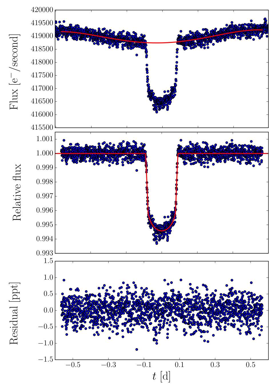
An example of the fit of a local stellar flux model, subsequent normalization of the transit, fit to a transit model, and resulting residuals is shown in Figure 2.
III.3 Changes in Crowding
Contamination of the photometric aperture by light from other stars also complicates accurate measurement of the transit depth. The PDC-MAP pipeline corrects this “crowding,” but time-varying errors in this procedure can produce changes in the measured transit depth. The process is analogous to star spots; the flux blocked by the planet is constant, but the estimated total flux from the star changes, yielding a change in the normalized transit depth. Van Eylen et al. [36] found that the transit depth of the hot Jupiter HAT-P-7b varied by from season to season,11 1 The Kepler Space Telescope performed an attitude adjustment four times per year to keep its solar panels pointed sunward. This causes each target to fall on a different CCD each “season.” orders of magnitude higher than the observed precision of transit depth measurements within a season. The authors suggested several possible causes, including incorrect crowding correction. Subsequently, Gandolfi et al. [15] found significant seasonal changes in transit depths measured from the PDC-MAP photometry of Kepler-423 (KOI 183). Since the changes in transit depths were highly correlated () with the quarterly22 2 Each change in Kepler season marks a new quarter, so data from Q1 and Q5 are from the same season, one year apart. crowding metric and were absent in the uncorrected SAP photometry, these authors attributed the changes entirely to the PDC-MAP crowding correction.
To screen for transit depth variations induced by crowding, we followed Gandolfi et al., and checked for correlation between measured transit depths and the quarterly crowding metric. Additionally, for each candidate, we generated two normalized light curves, using the default PDC-MAP quarter-to-quarter crowding correction and a constant seasonal crowding value.
III.4 Measuring Transit Depth
Transit models were then fit to the normalized light curves in a two-step process. We first phase-folded transits and fit a typical quadratic limb darkening transit model [25] using minimization. The initial values were taken from the NASA Exoplanet Archive.33 3 http://exoplanetarchive.ipac.caltech.edu Then, to extract the transit depths, we fixed the limb darkening model and orbital parameters, and fit between one and a few transits with only the radius ratio, , and transit mid-time, , as free parameters. The estimated error in each depth measurement was determined from propagation of the PDC pipeline estimated photometric error. The estimated transit depth errors varied from star to star, with a typical value of . Transits were rejected if the data coverage over the transit was too sparse or large data gaps prevented an accurate fit to the out-of-transit flux.
IV Determination of Oblateness
We examined the time series of measured transit depths for each candidate for signs of transit depth variations attributable to the spin precession of an oblate planet. To begin, we converted the series of measured transit depths into a time series of fractional transit depth variation, , from the mean observed depth.44 4 This definition is slightly different from that introduced in Carter and Winn [7], who normalized by the minimum transit depth. Because transit depths may vary systematically from season to season in Kepler photometry [36], we normalized the depths from each season by the mean of the observed depths from that season:
| (12) |
where the index indicates the season.
We constructed a corresponding model of the relative transit depth variation, m, using Equation (4) in Section II, in which we substituted for and using (3) and (5), respectively. As can be seen from these equations, this model has the precession period, , oblateness, , obliquity, , transit inclination, , and a phase offset, as free parameters. For a given choice of these parameters, we used Equation (4) to calculate the modeled transit depth, , at the observed transit times. We then normalized the modeled depths from each season by the mean of the modeled depths from that season as in Equation (12). Because we expect the planet-to-star radius ratio, , and the stellar limb darkening model to remain constant over the observation period, this normalization by makes both the observed and modeled series independent of these parameters.
IV.1 Fitting the Model
Fits of this model to transit depth time series are generally not unique. High oblateness, for example, can be compensated by very low obliquity or very slow precession. We explored this parameter space using emcee, a Markov chain Monte Carlo Ensemble sampler written by Foreman-Mackey et al. [14]. We used uniform priors over the appropriate physical range (e.g. ) for every model parameter but the transit inclination. The inclinations of our candidates were constrained by a normal prior based on the results of previous studies. For Kepler-39b we used [4], while for Kepler-427b our prior was [17].
We also restricted the precession period. First, we imposed a lower bound of 2 years. This is lower than expected for a Saturn-like planet on the inner-edge of our period range with modest rotational oblateness, , and reduced the likelihood of overfitting to sparse data or detecting a spurious signal associated with Kepler’s year orbit. Second, because of the finite duration of the observations, a planet model with significant oblateness can match even unvarying transit depth measurements if compensated by a long enough precession period. To avoid this degeneracy, we required that the precession period be short enough that we could have observed a rise and fall in the measured transit depths. Given the year duration of the Kepler mission, and that the transit depth variations peak twice per precession period, our final requirement was .
To test the robustness and reliability of our MCMC approach, for each candidate we performed two injection and recovery tests. The first test was a spherical planet. Because oblateness is a positive-definite quantity, our marginalized posterior distributions of will have positive bias (see, for example, Zakamska et al. [39]). The spherical planet test gauged the extent of the bias and probed for other possible false positive signals. The second injected planet was Saturn-like. It had oblateness , obliquity , the same transit inclination as the real candidate, and a precession period determined by Equation (8), assuming the same orbital period as the candidate, a 10 hour rotation period and . In both cases, the planets were scaled so that the transit depth matched that measured for the real candidate.
We ran our MCMC analysis with 200 parallel chains taking 15,000 steps. We discarded the first steps as the burn in period. We assessed convergence by inspection of the walker trajectories and by splitting the remaining part of the chain in half and comparing the resulting posteriors. The resulting MCMC model was determined by taking the median of the marginalized posterior distribution of each parameter with the 16th and 84th percentiles taken as approximate bounds.
IV.2 Statistical Significance
The likelihood function was calculated using the errors estimated for each transit as described in Section III. These estimates, however, may understate the true error. We performed a series of injection and recovery tests to assess our measurement accuracy and gauge the resulting false positive rate.
IV.2.1 Simulated Transit Light Curves
When Carter and Winn [7] investigated the detectability of transit depth variations in simulated Kepler photometry, they used a Gaussian white noise model with a simulated transit light curve. They found that a single transit’s depth could be recovered to within for a star with a Kepler magnitude of 13. With the full 4 years of data in hand, we attempted to improve this estimate by injecting transits into real Kepler photometry.
For each candidate, we constructed a series of simulated Kepler data sets using the photometry for that star. First, we removed all known transits from the data. We considered the remaining photometric data to consist of the true stellar flux plus some noise-induced offset: . We calculated the running average of the photometry and took this as our model for the stellar flux, . We then added artificial Mandel and Agol [25] transit models to the stellar flux: . The simulated data was then generated by applying the same offset that was present in the real data: .
After generating the artificial Kepler observations, we then fed the data into our analysis pipeline. We tested our analysis using both a constant and variable planet-to-star radius ratio to generate the injected transit models. For each star we generated simulated transits and compared our pipeline’s estimated error, derived from the Kepler pipeline’s reported photometric uncertainty, to the actual accuracy obtained from comparing the recovered transit parameters to the injected ones. We found that propagation of the photometric precision tends to underestimate the transit depth measurement error. An example of the error distribution is shown in Figure 3 for Kepler-39 (KOI 423).
IV.2.2 Simulated Transit Depth Series
Next, we investigated the false positive rate for oblateness detection using synthetic data. We generated time series for a spherical planet in two ways, by sampling from the error distributions described above and by bootstrapping from the observed series. To account for the possibility of seasonally correlated data, we used block bootstrapping; synthetic data for each season was resampled from that season’s observations. For each time series, we then calculated the value for the minimum- oblate planet model and a spherical planet model. These values were used to create both a simulated and bootstrapped distribution of values for that star. Given an oblate model fit to Kepler data and two distributions from simulated series, we calculate p-values from the fraction of simulated values higher than the one obtained by the model and report the more conservative estimate.
V Results
Of the 9 candidates matching our period criteria and having , we selected two, Kepler-39b (KOI 423.01) and Kepler-427b (KOI 192.01) for close evaluation based on their large transit depths () and independently measured masses. The results are presented below and summarized in Table 2.
V.1 Kepler-39b (KOI 423.01)
Zhu et al. [40] conducted a search for oblate planets using Kepler short cadence photometry to identify deviations from the light curve of a perfectly spherical transiting planet. The Kepler-39b (KOI 423.01) was the only object found with likely non-zero oblateness. Though the measured projected oblateness was high, , the authors cautioned that the finding might not be robust due to inconsistency in the best fit models when different subsets of short-cadence transits were examined.
With this tentative detection, and an orbital period of approximately 21 days, Kepler-39b presented a promising target for the method. We fit normalized transit models to 46 of the 69 transits spanning 3.93 years of long-cadence Kepler photometry. Kepler-39 is a star with a Kepler band magnitude of [4]. Due to the relative faintness of the star, the long cadence data has a photometric precision of . The standard deviation of errors in our signal, as determined by our injection and recovery test, was (see Figure 3). We found no correlation between the measured transit depth and the Kepler quarterly crowding metric.
The measured relative and the best-fit model are plotted in Figure 4. For visual clarity, we omitted the separate seasonal normalizations and show the variations relative to the mean of all the observed depths. The MCMC analysis yielded modest oblateness, , with a rapid precession period of . The full model is detailed in Table 2 and the posterior distributions are shown in Figure 9. The precession period is tightly bound at the lower edge of the range of allowed periods. The joint - distribution shows the expected degenerate relationship (Equation 6), with zero oblateness excluded and low oblateness allowed only at very high obliquities.
The cumulative distribution of values for the simulated ensemble of spherical planet models is shown in Figure 5. The recovered oblate model scored , corresponding to , or significant at the level.
We created similar distributions based on the simulated data we generated for injected spherical and Saturn-like planets. The p-values obtained from these distributions are also shown in Figure 5. The recovered model from the injected spherical planet had , or , indicating an oblate model provides no statistical advantage over a spherical planet model. The absence of a robust detection is corroborated by the posterior distributions shown in Figure 10. For and , we recovered our Gaussian and uniform priors, respectively. The posteriors for and display the expected degeneracy while the joint distribution shows that the data support models with near zero oblateness even for modest obliquity. The posterior spans the allowed range but has a broad peak in probability density centered near 6 years.
The recovered model for the Saturn-like planet was also not statistically significant, with , corresponding to . As before, the posterior distributions (Figure 10) reflect the absence of a detection, while in this case the posterior shows unexpected narrow peaks at periods of 2 and 3 years. The failure to detect the injected Saturn-like planet was not surprising, given that the injected period, , exceeds the upper limit we imposed on the precession period, but the high probability density at low periods was unexpected. This anomaly in the precession period posterior for the Saturn-like case occurs at roughly the same period as the signal in the real photometry, suggesting that detection may be spurious.
V.2 Kepler-427b (KOI 192.01)
Kepler-427 (KOI 192), is a star hosting a planet on a 10.3 day orbit [17]. Like Kepler-39, Kepler-427 is a relatively dim star with a Kepler band magnitude of [17], resulting in photometric precision of approximately . From recovery of simulated transits we obtained a standard deviation of errors (see Figure 6). Again we find no significant correlation between the Kepler quarterly crowding metric and the observed transit depths.
We fit 104 long-cadence transits spanning nearly 4 years of Kepler photometry, with the resulting relative measurements and the best-fit model plotted in Figure 7. The oblate planet model had , which, in comparison to the distribution shown in Figure 8, yields , or . From the MCMC posterior distributions (Figure 12) we obtained with a precession period of .
The model recovered for the simulated spherical planet matches the expectation for unvarying transit depths. The posterior distributions (Figure 13) largely recover the input priors, with the familiar degenerate structure for and . The posterior distribution of precession period shows a short-period peak analogous to that recorded in the Saturn-like simulation for Kepler-39b. The oblate model fit is not significant, scoring , or , indicating no improvement on a spherical model.
In the case of the simulated Saturn-like planet, the oblate model is a highly significant improvement on a spherical planet fit, achieving or . In addition, with the exception of the precession period, all the input parameters were recovered in the estimated 68% confidence interval (see Figure 14). The precession period was only narrowly outside the interval. The poorly resolved period is likely due to the 4 year duration of data compared to the 7.23 year injected period. We recovered to within 12.5% of the input value, but, in part due to the - degeneracy (Equation 6), we only recovered to within 50% and to within 35%.
| Planet | |||||
|---|---|---|---|---|---|
| Kepler-39b | |||||
| Kepler-427b | |||||
| Kepler-39 (KOI 423.01) Simulated Planets | |||||
| Spherical (Injected) | |||||
| Spherical (Recovered) | |||||
| Saturn-like (Injected) | |||||
| Saturn-like (Recovered) | |||||
| Kepler-427 (KOI 192.01) Simulated Planets | |||||
| Spherical (Injected) | |||||
| Spherical (Recovered) | |||||
| Saturn-like (Injected) | |||||
| Saturn-like (Recovered) | |||||
Note. — The reported values are the medians along with the 16th and 84th percentiles.
The recovery of an injected candidate and the absence of a false positive detection in the null simulation indicate that the confidence level of the recovered signal in the real Kepler data is likely valid.
To confirm that the observed change in transit depth was not a byproduct of our transit normalization technique, we repeated our analysis with the starspot correction (Section III.2) removed. Kepler-427 only showed starspot-like brightness fluctuations in a few quarters. As a consequence, the average change in recovered transit depths was only , less than 0.1% of the transit depth. The change in measured depths affected the model recovered from our MCMC analysis, but for each parameter, the recovered values with or without the starspot correction are mutually consistent—the median value obtained with one method is within the estimated uncertainty of the median value obtained with the other normalization. In particular, the measured precession period changed by 0.5%, while changed by 7%. Finally, removing the starspot correction marginally diminishes the statistical significance of the detection, yielding or . Based on these findings, we conclude that the observed signal is not an artifact of our normalization procedure.
VI Discussion
In this paper, we present the first attempt to detect the rotational oblateness of an exoplanet through long-term changes in transit depth. We examined confirmed Kepler planets with periods between 10 and 30 days and radii greater than for signs of transit depth variations consistent with the spin-axis precession of an oblate planet. Of the 9 planets matching our criteria, we selected two for close analysis, Kepler-39b (KOI 423.01) and Kepler-427b (KOI 192.01). We searched for an oblate signature using a Markov Chain Monte Carlo approach and assessed the significance of the recovered oblate planet fits.
VI.1 Kepler-39b (KOI 423.01)
Although we detected oblateness () with high significance in Kepler-39b, based on the additional injection and recovery tests, this detection is likely a false positive. The posterior distributions of precession period recovered from the true and Saturn-like simulated Kepler-39 photometry (Figures 9, 11) both show excess probability mass at low periods. The recovered 2.04 year period is exactly twice the 372.5 day Kepler orbit and suggests an explanation. For , the peaks have comparable amplitude, creating a quasi-periodic signal matching the Kepler year. While we have corrected for sharp changes in transit depth at quarter boundaries caused by the spacecraft’s seasonal rolls (see Section III.3), other systematics have been observed. In a study of M giant variability, Bányai et al. [1] found one quarter of their targets exhibited smooth flux variations with 372.5 day periods. The high statistical significance (, ) of the observed transit depth variations may reflect detection of this effect or another similar systematic.
The physical plausibility of such rapid precession casts additional doubt on our detection. Assuming the detected oblateness to be rotationally induced, we can calculate the required rotation rate and estimated precession period using Equations (2) and (8). Bonomo et al. [4] recently updated the parameters for the Kepler-39 system. They find that the previously measured eccentricity may be spurious, so we adopt the values from the circular model for simplicity: and a mean radius . For planets in hydrostatic equilibrium, we can apply the Darwin-Radau approximation [27]:
| (13) |
Assuming, conservatively, that , corresponding to a uniform density sphere, then and the required rotation period to produce the measured oblateness is . The resulting precession period is . Under the more common assumption that for giant planets, . Relaxing the Darwin-Radau constraint, assuming the observed oblateness can be supported at , and that , the observed precession period requires , considerably less than the value of 13.5 for Saturn [38].
The presence of exomoons around Kepler-39b could alter the effective value of and drive faster precession; Saturn’s satellites reduce its calculated precession period by a factor of 4 [7]. The effective value of is given by where
| (14) | |||
| (15) |
where , , , and are the satellite’s mass, semimajor axis, orbital period and inclination relative to the planet’s equator [38]. Prograde satellites on circular orbits are only stable with a semimajor axis [13, 32]. Under the generous (and inconsistent) assumptions that (corresponding to in the Darwin-Radau relationship), , and that the satellite has , then the required reduction in is achieved at . By comparison, Jupiter and Saturn’s largest satellites, Ganymede and Titan, have masses of and , respectively [34, 23], and each orbit at times the Hill radius of their respective hosts. Modeling satellite formation around gas giants, Canup and Ward [5] find that competing processes naturally limit satellite systems to a total mass of , or for Kepler-39b. A massive satellite of Kepler-39b, therefore, seems to be an unlikely explanation for the observed precession period.
If our detection is indeed a false positive, these results are consistent with the findings of Zhu et al. [40]. Using their assumptions and measured values of and , we obtain an expected precession period of years, much longer than could be detected from 4 years of Kepler observations. Updated measurements of the Kepler-39 system [4] have reduced the age estimate from to (or if the observed eccentricity is real), greatly decreasing the time available to de-spin the planet and bolstering the claim that the rapid rotation could be primordial.
VI.2 Kepler-427b (KOI 192.01)
We detected variation in the transit depths of Kepler-427b consistent with moderate oblateness () at a significance level of . In contrast to Kepler-39b, we do not believe this to be a data artifact. While the simulated null case does show an excess of probability density at short precession periods, there is no indication of this signal in the recovered distributions for the Saturn-like case or the real data. Furthermore, the solutions found for the real data and Saturn-like planet are not located in the same region of parameter space as the signal found for the null case.
If the observed signal is caused by spin precession, then armed with the measured oblateness and precession period, and assuming the Darwin-Radau approximation, we can infer a range of values for , and . Adopting and from Hébrard et al. [17], we find , , and . By comparison, Jupiter has and a rotation rate of .55 5 http://ssd.jpl.nasa.gov/?gravity_fields_op The detailed interior structure of Jupiter is still uncertain, but common model-derived values for the normalized moment of inertia are [21]. Saturn, with nearly the same mass as Kepler-427b, has [23] and a rotation period of . Hubbard and Marley [20] present an interior model for Saturn with while Ward and Hamilton [38] propose a dynamical origin for Saturn’s obliquity which requires . Most of the range of our inferred values is outside that expected from Solar System gas giants, but there is some overlap.
The rotation period we measure is significantly shorter than the orbital period of the planet. Using Equation (10), assuming an initial rotation period of , near the breakup rotation rate, and an optimistic tidal dissipation factor, , we calculate that only are required to spin down Kepler-427b to the rotation periods inferred by our measurement. This is much shorter than the estimated system age of , an apparent contradiction. Equation (10) is highly approximate, and is derived assuming a circular orbit and a planet with its spin axis aligned to the orbit normal. Planets on eccentric orbits do not directly synchronize, instead entering a quasi-synchronous spin state while they retain significant eccentricity [12]. Hébrard et al. [17] were not able to significantly measure the eccentricity of Kepler-427b, providing only a upper bound of . Kepler-427b lies in the “period valley”—the sparsely populated region between hot Jupiters and more distant gas giant planets ()—making tidal circularization a precarious assumption. Hébrard et al. suggest that follow up measurements could more precisely constrain the orbital eccentricity, stellar age and radius, and the planetary radius, potentially resolving the spin-down time problem.
VI.3 Other Causes of Transit Variations
Changes in the transit geometry can also alter the measured transit depth. To confirm our confidence level we examined several possible sources of false positives.
VI.3.1 Nodal Precession
If Kepler-427b is undergoing sufficiently rapid nodal precession—the precession of the orbital plane—the impact parameter of the transit would change during our observations. In conjunction with limb darkening, this would change the measured transit depth over time. The nodal precession rate is given by
| (16) |
where is the angle between the orbit normal and the spin axis of the star and is the star’s zonal quadrupole moment [27, 3]. For the Kepler-427 system, , and [17]. For the stellar quadrupole moment, we adopted the Sun-like value [35, 26]. Assuming, conservatively, that and that the eccentricity is near the upper bound, , we obtain . This is a nodal precession period of , too slow to account for the observed changes in transit depth.
VI.3.2 Apsidal Precession
If Kepler-427b is on an eccentric orbit, then apsidal precession, or periastron precession, would change the star-planet distance during the transit over time. If the transit is not observed edge-on, this would cause the transit impact parameter, and observed transit depth, to change over time. Ragozzine and Wolf [28] calculated the expected apsidal precession rate for a hot Jupiter. Following their formulation, we find the dominant term is precession driven by the planet’s rotational bulge:
| (17) |
where is the planet’s Love number. Assuming , , and a Saturn-like Love number, [24], we calculate . To include the remaining terms from Ragozzine and Wolf, we assumed a stellar rotation period of , appropriate for Sun-like stars with ages of [11], and consistent with , measured by Hébrard et al. [17]. Following Ragozzine and Wolf, we adopted a stellar Love number . Under these assumptions, the total precession induced is . This includes, in order of diminishing importance, the effects of the rotational bulge of the planet, the tidal bulge on the planet, general relativity, the rotational bulge of the star, and the tidal bulge on the star. The corresponding apsidal precession period of is too long to explain the observed change in transit depth.
VI.3.3 Three Body Interactions
The preceding calculations only considered a two-body system. Dynamical interactions with another planet in the Kepler-427 system could drive faster precession or create secular variation in the eccentricity or inclination of Kepler-427b’s orbit. While we cannot definitively exclude this possibility, we found no evidence of timing variations in the transits of Kepler-427b, consistent with the TTV survey of the entire Kepler data set undertaken by Holczer et al. [18]. Additionally, no evidence of another companion is reported in the HARPS-N spectrograph observations conducted by Hébrard et al. [17].
Given the expected long precession periods and lack of evidence for strong interactions with another body, we conclude that changes in orbital geometry are not the cause of the observed transit depth variations, and that the confidence estimate is reliable.
VI.4 Conclusion
We have presented the first attempt at detecting the oblateness of an exoplanet through changes in transit depth caused by spin precession. We examined two planets in detail. While we were unable to detect the oblateness of Kepler-39b, this is broadly consistent with the findings of Zhu et al. [40] given the expected long precession period. We find transit depth changes consistent with an oblateness comparable to Solar System gas giants for Kepler-427b, but with a significance of only (). Kepler-427b is a warm Saturn in the period-valley (), a class of planets with an unclear formation mechanism [31]. Confirming and improving this oblateness detection and further constraining the bulk properties of Kepler-427b would illuminate the planet’s internal structure, possibly providing insight into period-valley giant planet formation, making the Kepler-427 system an attractive target for followup observations.
Current and near-future missions, such as K2 [19] using Kepler and the Transiting Exoplanet Survey Satellite [29], probably do not have the long time baseline required to detect these transit depth variations. TESS, however, is likely to provide a wealth of more easily characterizable targets in the period range where these effects are measurable, allowing for long-term followup using other instruments. Additionally, TESS’s high quality short-cadence photometry will provide a rich dataset for the method attempted by Carter and Winn [6] and Zhu et al. [40]. Efforts combining both methods promise to greatly expand our understanding of gas giant structure and formation.
References
- [1] E. Bányai, L. L. Kiss, T. R. Bedding, B. Bellamy, J. M. Benkő, A. Bódi, J. R. Callingham, D. Compton, I. Csányi, A. Derekas, J. Dorval, D. Huber, O. Shrier, A. E. Simon, D. Stello, G. M. Szabó, R. Szabó, and K. Szatmáry. Variability of M giant stars based on Kepler photometry: general characteristics. MNRAS, 436:1576–1587, December 2013. 10.1093/mnras/stt1685.
- [2] J. W. Barnes and J. J. Fortney. Measuring the Oblateness and Rotation of Transiting Extrasolar Giant Planets. ApJ, 588:545–556, May 2003. 10.1086/373893.
- [3] J. W. Barnes, J. C. van Eyken, B. K. Jackson, D. R. Ciardi, and J. J. Fortney. Measurement of Spin-orbit Misalignment and Nodal Precession for the Planet around Pre-main-sequence Star PTFO 8-8695 from Gravity Darkening. ApJ, 774:53, September 2013. 10.1088/0004-637X/774/1/53.
- [4] A. S. Bonomo, A. Sozzetti, A. Santerne, M. Deleuil, J.-M. Almenara, G. Bruno, R. F. Díaz, G. Hébrard, and C. Moutou. Improved parameters of seven Kepler giant companions characterized with SOPHIE and HARPS-N. A&A, 575:A85, March 2015. 10.1051/0004-6361/201323042.
- [5] R. M. Canup and W. R. Ward. A common mass scaling for satellite systems of gaseous planets. Nature, 441:834–839, June 2006. 10.1038/nature04860.
- [6] J. A. Carter and J. N. Winn. Empirical Constraints on the Oblateness of an Exoplanet. ApJ, 709:1219–1229, February 2010a. 10.1088/0004-637X/709/2/1219.
- [7] J. A. Carter and J. N. Winn. The Detectability of Transit Depth Variations Due to Exoplanetary Oblateness and Spin Precession. ApJ, 716:850–856, June 2010b. 10.1088/0004-637X/716/1/850.
- [8] J. A. Carter, J. N. Winn, M. J. Holman, D. Fabrycky, Z. K. Berta, C. J. Burke, and P. Nutzman. The Transit Light Curve Project. XIII. Sixteen Transits of the Super-Earth GJ 1214b. ApJ, 730:82, April 2011. 10.1088/0004-637X/730/2/82.
- [9] J. L. Christiansen, J. M. Jenkins, D. A. Caldwell, T. Barclay, S. T. Bryson, C. J. Burke, J. Campbell, J. Catanzarite, B. D. Clarke, J. L. Coughlin, F. Girouard, M. R. Haas, K. Ibrahim, T. C. Klaus, J. J. Kolodziejczak, J. Li, S. D. McCauliff, R. L. Morris, F. Mullally, E. V. Quintana, J. Rowe, A. Sabale, S. Seader, J. C. Smith, M. D. Still, P. G. Tenenbaum, S. E. Thompson, J. D. Twicken, and A. K. Uddin. Kepler data characteristics handbook (ksci-19040-004), 2013.
- [10] S. Czesla, K. F. Huber, U. Wolter, S. Schröter, and J. H. M. M. Schmitt. How stellar activity affects the size estimates of extrasolar planets. A&A, 505:1277–1282, October 2009. 10.1051/0004-6361/200912454.
- [11] J.-D. do Nascimento, Jr., R. A. García, S. Mathur, F. Anthony, S. A. Barnes, S. Meibom, J. S. da Costa, M. Castro, D. Salabert, and T. Ceillier. Rotation Periods and Ages of Solar Analogs and Solar Twins Revealed by the Kepler Mission. ApJ, 790:L23, August 2014. 10.1088/2041-8205/790/2/L23.
- [12] I. Dobbs-Dixon, D. N. C. Lin, and R. A. Mardling. Spin-Orbit Evolution of Short-Period Planets. ApJ, 610:464–476, July 2004. 10.1086/421510.
- [13] R. C. Domingos, O. C. Winter, and T. Yokoyama. Stable satellites around extrasolar giant planets. MNRAS, 373:1227–1234, December 2006. 10.1111/j.1365-2966.2006.11104.x.
- [14] D. Foreman-Mackey, D. W. Hogg, D. Lang, and J. Goodman. emcee: The mcmc hammer. PASP, 125:306–312, 2013. 10.1086/670067.
- [15] D. Gandolfi, H. Parviainen, H. J. Deeg, A. F. Lanza, M. Fridlund, P. G. Prada Moroni, R. Alonso, T. Augusteijn, J. Cabrera, T. Evans, S. Geier, A. P. Hatzes, T. Holczer, S. Hoyer, T. Kangas, T. Mazeh, I. Pagano, L. Tal-Or, and B. Tingley. Kepler-423b: a half-Jupiter mass planet transiting a very old solar-like star. A&A, 576:A11, April 2015. 10.1051/0004-6361/201425062.
- [16] P. Goldreich and S. Soter. Q in the Solar System. Icarus, 5:375–389, 1966. 10.1016/0019-1035(66)90051-0.
- [17] G. Hébrard, A. Santerne, G. Montagnier, G. Bruno, M. Deleuil, M. Havel, J.-M. Almenara, C. Damiani, S. C. C. Barros, A. S. Bonomo, F. Bouchy, R. F. Díaz, and C. Moutou. Characterization of the four new transiting planets KOI-188b, KOI-195b, KOI-192b, and KOI-830b. A&A, 572:A93, December 2014. 10.1051/0004-6361/201424268.
- [18] T. Holczer, T. Mazeh, G. Nachmani, D. Jontof-Hutter, E. B. Ford, D. Fabrycky, D. Ragozzine, M. Kane, and J. H. Steffen. Transit Timing Observations from Kepler. IX. Catalog of the Full Long-cadence Data Set. ApJS, 225:9, July 2016. 10.3847/0067-0049/225/1/9.
- [19] S. B. Howell, C. Sobeck, M. Haas, M. Still, T. Barclay, F. Mullally, J. Troeltzsch, S. Aigrain, S. T. Bryson, D. Caldwell, W. J. Chaplin, W. D. Cochran, D. Huber, G. W. Marcy, A. Miglio, J. R. Najita, M. Smith, J. D. Twicken, and J. J. Fortney. The K2 Mission: Characterization and Early Results. PASP, 126:398, April 2014. 10.1086/676406.
- [20] W. B. Hubbard and M. S. Marley. Optimized Jupiter, Saturn, and Uranus interior models. Icarus, 78:102–118, March 1989. 10.1016/0019-1035(89)90072-9.
- [21] W. B. Hubbard and B. Militzer. A Preliminary Jupiter Model. ApJ, 820:80, March 2016. 10.3847/0004-637X/820/1/80.
- [22] L. Hui and S. Seager. Atmospheric Lensing and Oblateness Effects during an Extrasolar Planetary Transit. ApJ, 572:540–555, June 2002. 10.1086/340017.
- [23] R. A. Jacobson, P. G. Antreasian, J. J. Bordi, K. E. Criddle, R. Ionasescu, J. B. Jones, R. A. Mackenzie, M. C. Meek, D. Parcher, F. J. Pelletier, W. M. Owen, Jr., D. C. Roth, I. M. Roundhill, and J. R. Stauch. The Gravity Field of the Saturnian System from Satellite Observations and Spacecraft Tracking Data. AJ, 132:2520–2526, December 2006. 10.1086/508812.
- [24] V. Lainey, R. A. Jacobson, R. Tajeddine, N. J. Cooper, C. Murray, V. Robert, G. Tobie, T. Guillot, S. Mathis, F. Remus, J. Desmars, J.-E. Arlot, J.-P. De Cuyper, V. Dehant, D. Pascu, W. Thuillot, C. Le Poncin-Lafitte, and J.-P. Zahn. New constraints on Saturn’s interior from Cassini astrometric data. Icarus, 281:286–296, January 2017. 10.1016/j.icarus.2016.07.014.
- [25] K. Mandel and E. Agol. Analytic Light Curves for Planetary Transit Searches. ApJ, 580:L171–L175, December 2002. 10.1086/345520.
- [26] R. Mecheri, T. Abdelatif, A. Irbah, J. Provost, and G. Berthomieu. New values of gravitational moments J2 and J4 deduced from helioseismology. Sol. Phys., 222:191–197, August 2004. 10.1023/B:SOLA.0000043563.96766.21.
- [27] C. D. Murray and S. F. Dermott. Solar system dynamics. 1999.
- [28] D. Ragozzine and A. S. Wolf. Probing the Interiors of very Hot Jupiters Using Transit Light Curves. ApJ, 698:1778–1794, June 2009. 10.1088/0004-637X/698/2/1778.
- [29] G. R. Ricker, J. N. Winn, R. Vanderspek, D. W. Latham, G. Á. Bakos, J. L. Bean, Z. K. Berta-Thompson, T. M. Brown, L. Buchhave, N. R. Butler, R. P. Butler, W. J. Chaplin, D. Charbonneau, J. Christensen-Dalsgaard, M. Clampin, D. Deming, J. Doty, N. De Lee, C. Dressing, E. W. Dunham, M. Endl, F. Fressin, J. Ge, T. Henning, M. J. Holman, A. W. Howard, S. Ida, J. M. Jenkins, G. Jernigan, J. A. Johnson, L. Kaltenegger, N. Kawai, H. Kjeldsen, G. Laughlin, A. M. Levine, D. Lin, J. J. Lissauer, P. MacQueen, G. Marcy, P. R. McCullough, T. D. Morton, N. Narita, M. Paegert, E. Palle, F. Pepe, J. Pepper, A. Quirrenbach, S. A. Rinehart, D. Sasselov, B. Sato, S. Seager, A. Sozzetti, K. G. Stassun, P. Sullivan, A. Szentgyorgyi, G. Torres, S. Udry, and J. Villasenor. Transiting Exoplanet Survey Satellite (TESS). Journal of Astronomical Telescopes, Instruments, and Systems, 1(1):014003, January 2015. 10.1117/1.JATIS.1.1.014003.
- [30] R. Sanchis-Ojeda, J. N. Winn, G. W. Marcy, A. W. Howard, H. Isaacson, J. A. Johnson, G. Torres, S. Albrecht, T. L. Campante, W. J. Chaplin, G. R. Davies, M. N. Lund, J. A. Carter, R. I. Dawson, L. A. Buchhave, M. E. Everett, D. A. Fischer, J. C. Geary, R. L. Gilliland, E. P. Horch, S. B. Howell, and D. W. Latham. Kepler-63b: A Giant Planet in a Polar Orbit around a Young Sun-like Star. ApJ, 775:54, September 2013. 10.1088/0004-637X/775/1/54.
- [31] A. Santerne, C. Moutou, M. Tsantaki, F. Bouchy, G. Hébrard, V. Adibekyan, J.-M. Almenara, L. Amard, S. C. C. Barros, I. Boisse, A. S. Bonomo, G. Bruno, B. Courcol, M. Deleuil, O. Demangeon, R. F. Díaz, T. Guillot, M. Havel, G. Montagnier, A. S. Rajpurohit, J. Rey, and N. C. Santos. SOPHIE velocimetry of Kepler transit candidates. XVII. The physical properties of giant exoplanets within 400 days of period. A&A, 587:A64, March 2016. 10.1051/0004-6361/201527329.
- [32] H. E. Schlichting and R. Sari. The Ratio of Retrograde to Prograde Orbits: A Test for Kuiper Belt Binary Formation Theories. ApJ, 686:741-747, October 2008. 10.1086/591073.
- [33] S. Seager and L. Hui. Constraining the Rotation Rate of Transiting Extrasolar Planets by Oblateness Measurements. ApJ, 574:1004–1010, August 2002. 10.1086/340994.
- [34] Adam P. Showman, Malhotra, and Renu. The galilean satellites. Science, 286(5437):77–84, 1999. ISSN 0036-8075. 10.1126/science.286.5437.77. URL http://science.sciencemag.org/content/286/5437/77.
- [35] R. K. Ulrich and G. W. Hawkins. The Solar Gravitational Figure - j2 and J4. ApJ, 246:985, June 1981. 10.1086/158992.
- [36] V. Van Eylen, M. Lindholm Nielsen, B. Hinrup, B. Tingley, and H. Kjeldsen. Investigation of Systematic Effects in Kepler Data: Seasonal Variations in the Light Curve of HAT-P-7b. ApJ, 774:L19, September 2013. 10.1088/2041-8205/774/2/L19.
- [37] W. R. Ward. Past orientation of the lunar spin axis. Science, 189:377–379, August 1975. 10.1126/science.189.4200.377.
- [38] W. R. Ward and D. P. Hamilton. Tilting Saturn. I. Analytic Model. AJ, 128:2501–2509, November 2004. 10.1086/424533.
- [39] N. L. Zakamska, M. Pan, and E. B. Ford. Observational biases in determining extrasolar planet eccentricities in single-planet systems. MNRAS, 410:1895–1910, January 2011. 10.1111/j.1365-2966.2010.17570.x.
- [40] W. Zhu, C. X. Huang, G. Zhou, and D. N. C. Lin. Constraining the Oblateness of Kepler Planets. ApJ, 796:67, November 2014. 10.1088/0004-637X/796/1/67.


