Radiation Transfer of Models of Massive Star Formation. IV. The Model Grid and Spectral Energy Distribution Fitting
Abstract
We present a continuum radiative transfer model grid for fitting observed spectral energy distributions (SEDs) of massive protostars. The model grid is based on the paradigm of core accretion theory for massive star formation with pre-assembled gravitationally-bound cores as initial conditions. In particular, following the Turbulent Core Model, initial core properties are set primarily by their mass and the pressure of their ambient clump. We then model the evolution of the protostar and its surround structures in a self-consistent way. The model grid contains about 9000 SEDs with 4 free parameters: initial core mass, the mean surface density of the environment, the protostellar mass, and the inclination. The model grid is used to fit observed SEDs via minimization, with the foreground extinction additionally estimated. We demonstrate the fitting process and results using the example of massive protostar G35.20-0.74. Compared with other SED model grids currently used for massive star formation studies, in our model grid, the properties of the protostar and its surrounding structures are more physically connected, which reduces the dimensionality of the parameter spaces and the total number of models. This excludes possible fitting of models that are physically unrealistic or that are not internally self-consistent in the context of the Turbulent Core Model. Thus, this model grid serves not only as a fitting tool to estimate properties of massive protostars, but also as a test of core accretion theory. The SED model grid is publicly released with this paper.
Keywords:
dust, extinction - ISM: clouds - radiative transfer - stars: formation - stars: massiveI Introduction
Massive stars impact many areas of astrophysics, yet there is still no consensus on how they form. Theories range from Core Accretion models, i.e., scaled-up versions of low-mass star formation (e.g., the Turbulent Core Model of McKee & Tan 32, McKee & Tan 33), to Competitive Accretion models at the crowded centers of forming star clusters (e.g., Bonnell et al. 9; Wang et al. 50), to Protostellar Collisions (Bonnell et al. 10; Bally & Zinnecker 4). Such confusion is partly due to the observational difficulties caused by the relative rarity and the typically large distances ( kpc) of massive protostars, highly crowded environments, and high extinctions. The environments of massive star formation are observed to be massive, dense gas clumps with mass surface densities of , which corresponds to a visual extinction of about mag (e.g., see Tan et al. 46 for a review).
Analysis of broad-band spectral energy distributions (SED) composed of total fluxes from NIR to FIR/sub-mm of massive protostars, via radiative transfer (RT) modeling, is a primary way to understand the properties of massive protostars, being efficient for large samples. A number of RT models have been developed to compare with observations. Robitaille et al. [40], Robitaille et al. [41] developed a large model grid to fit the SEDs of young stellar objects (YSOs). However, their model grid was mainly developed for low-mass star formation, without coverage of the parameter space needed for massive star formation, such as very high accretion rates resulting from high mass surface density environments. A similar RT model grid has also been developed by Molinari et al. [35], which focused on massive YSOs. However, the components in their model are relatively simple. A massive YSO involves complicated structures such as the protostar, accretion disk, envelope and outflow, each of which may need multiple parameters to define their properties that may affect the resulting SED. Therefore, to fit an observed SED usually requires setting a large number of independent parameters. This is the method that the above mentioned model grids have adopted. While the wide choice of free parameters can generate good fits to the observations, such a method usually also generates results that are physically less realistic or not self-consistent (see, e.g., De Buizer et al. 15). Large numbers of free parameters will also lead to higher susceptibility to degeneracies.
In this paper, the fourth of our series, we aim to use a different approach to build the model grid. Instead of large numbers of free parameters, we make the components more physically connected to reduce the number of independent parameters. Our model grid is based on a particular model of massive star formation, the Turbulent Core model (McKee & Tan 32, McKee & Tan 33). In the Turbulent Core model, massive stars are formed from pre-assembled massive pre-stellar cores, supported by internal pressure that is provided by a combination of turbulence and magnetic fields. The pressure at the core surface is assumed to be approximately the same as that of the surrounding larger-scale star-cluster-forming clump, with a typical mean mass surface density of . We construct the model grid from two initial conditions, the initial core mass, , and environmental mass surface density, . With various analytical or semi-analytical solutions, we calculate the properties of different components including the protostar, disk, envelope, outflow and their evolutions self-consistently from the initial conditions. The main free parameters in this model grid are the initial conditions, i.e., and , and the protostellar mass indicating the evolutionary stage, as well as the inclination and foreground extinction from the larger clump. In such a method, the model grid will exclude certain combinations of the components which are not supported by the core accretion theory. By fitting the observed SEDs, this model will allow us to see whether the observed variety of massive protostars can be explained by a scenario of core accretion in different evolutionary stages and initial/environmental conditions.
In the previous papers in our series (Zhang & Tan 55, hereafter Paper I; Zhang et al. 58, hereafter Paper II; Zhang et al. 59, hereafter Paper III), we studied a fiducial case of a massive protostar growing inside a core with an initial mass of and in a environment, and a few variants of it. Now in this paper, we present the full model grid covering a large parameter space, and investigate how the initial conditions and evolution affect the SEDs of massive protostars (§2). We develop an SED fitting tool to fit observed SEDs with this model grid (§3). In §4, we demonstrate the fitting process and results using the SED of the massive protostar G35.20-0.74 as an example. We discuss our results and present conclusions in §5.
II Model Grid
II.1 Physical Model
We first briefly describe the physical assumptions used in our models, which have been introduced in the previous papers in this series. For detailed derivation and discussion of these points, please refer to Papers I, II and III. Following McKee & Tan [33], a star-forming core is defined as a region of a molecular cloud that forms a single star or a close binary via gravitational collapse. We can define such cores to contain a single, central rotationally-supported disk. The initial core is assumed to be quasi-spherical, self-gravitating, in near virial equilibrium, and in pressure equilibrium with the surrounding star-cluster forming clump. The size of such a core is determined by the mean mass surface density of the surrounding clump (which sets the pressure on the boundary of the core) by
| (1) |
(McKee & Tan 33). In the following text, is also referred to as the mass surface density of the star-forming environment. The density distribution in the initial core is described by a power law in spherical radius, . Observations suggest has a mean value of 1.3 to 1.6 (Butler & Tan 11; Butler et al. 12). Therefore we adopt a fiducial value of for the whole model grid, which is also consistent with our previous studies and the Turbulent Core Model by McKee & Tan [33].
The collapse of the core is described by an inside-out solution (Shu 45; McLaughlin & Pudritz 30, McLaughlin & Pudritz 31), together with the effect of rotation (Ulrich 49). Disks around massive protostars are also expected to be massive due to the high accretion rates of about to (e.g., Beltrán & de Wit 6). We assume the mass ratio between the disk and the protostar is a constant , considering the rise in effective viscosity due to disk self-gravity at about this value of (Kratter et al. 27). Disk size is calculated from the rotating collapse of the core to be , where is the mass of the star-disk system in the limit of no feedback as calculated from the collapse solution, and is the actual mass in the star-disk system (see Paper III). The rotational-to-gravitational energy ratio of the initial core is assumed to be 0.02, which is a typical value from observations of low and high-mass prestellar cores (e.g. Goodman et al. 21; Li et al. 28; Palau et al. 38). The disk structure is described with an “-disk” solution (Shakura & Sunyaev 44), with an improved treatment to include the effects of the outflow and the accretion infall to the disk (Paper II). Half of the accretion energy is released when the accretion flow reaches the stellar surface (i.e., the boundary layer luminosity, ). We assume this part of the luminosity is radiated together with the intrinsic stellar luminosity isotropically as a single black-body, i.e., the total luminosity from the protostar is and the surface temperature of the protostar is . The other half of the accretion energy is partly radiated from the disk during accretion and partly converted to the kinetic energy of the disk wind. The total amount and the detailed distribution of the accretion energy radiated from the disk are simultaneously derived from the disk solution.
The density distribution of the disk wind is described by a semi-analytic solution, which is approximately a Blandford & Payne [8] wind (see Appendix B of Paper II), and the mass loading rate of the wind relative to the stellar accretion rate is assumed to be , which is a typical value for disk winds (Königl & Pudritz 26). Such a disk wind carves out polar cavities in the core, which gradually open up as the protostar evolves. The opening angle of the outflow cavity is estimated following the method of Matzner & McKee [29] by comparing the wind momentum and that needed to accelerate the core material to its escape velocity (Paper III). The accretion rate to the protostar is regulated by such outflow feedback. Note that we allow existence of dust in some regions of the outflow cavity if the disk winds in these regions originate from the disk outside of the dust sublimation front.
The evolution of the protostar is solved using the model by Hosokawa & Omukai [23] and Hosokawa et al. [24]. The model solves the detailed internal structure of the protostar, such as the deuterium burning region, convective zone, and radiative zone, from the accretion history calculated above (see Paper III for more details). A photospheric boundary condition, which is usually associated with the situation of disk accretion, is used in the protostellar evolution calculation. Several outputs of this calculation that are important for setting up our grid of physical models for radiative transfer computation include the evolution of protostellar radius, luminosity and surface temperature with the protostellar mass.


II.2 Parameter Space
In such a framework, the evolution of the core, protostar, disk and outflow cavity are self-consistently calculated from two main initial conditions of the core: its initial mass () and the mean mass surface density of the clump that the core is embedded in (). We refer to the evolutionary history of protostar from a given set of initial conditions as an evolutionary track, and a particular moment on such a track as an evolutionary stage, which is specified by a third parameter, the protostellar mass . We refer to the entire set of tracks as the model grid. Therefore, this model grid is of three dimensions (). In the current model grid, is sampled at 10, 20, 30, 40, 50, 60, 80, 100, 120, 160, 200, 240, 320, 400, 480 , and is sampled at 0.1, 0.32, 1, 3.2 , forming 60 evolutionary tracks. is sampled at 0.5, 1, 2, 4, 8, 12, 16, 24, 32, 48, 64, 96, 128, 160 . Note that for each track, not all of these are sampled. In particular, the maximum protostellar mass is limited by the final stellar mass achieved in a given evolutionary track (see Figure 3). As a result, there are totally 432 different physical models defined by different sets of .
We note that other initial conditions may affect the models, such as the initial rotational-to-gravitational energy ratio of the core and magnetic field strength in the core, both of which are expected to influence the size of the accretion disk. However, the spectral energy distributions are not significantly affected by variations of the disk size about its fiducial values, given that the disk is always large compared to the size of the star and small compared to the extent of the core and outflow cavities (see Paper III).
Figure 1 shows the range of the initial conditions in our model grid. The mass surface density of the star-forming environment, , covers a range from to . This range is similar to the values found in most Galactic massive star forming regions, including: infrared dark clouds (IRDCs, dark green squares) and their internal clumps/cores (dark green crosses) that are thought to represent the initial stage of massive star formation; massive star-forming clumps/cores (red squares and light green circles), including those at Galactic Center (e.g., the “Brick”); some massive star clusters (e.g., the Orion Nebula Cluster [ONC]) and even more massive “super star clusters” (e.g., Westerlund 1, Arches, and Quintuplet). The initial core mass, , in the model grid covers a range from to about , which is similar to those of individual pre-stellar and protostellar cores inside IRDCs and massive clumps. Therefore, our model grid covers a wide range of initial conditions that are suitable to form individual stars from intermediate to high-mass. We note that as the first release of the model grid, the current version does not have very fine sampling over the initial conditions, especially the surface density of the star-forming environment . While the sampling of in the current model grid, which covers most of the relevant range of local massive star formation, is sufficient to understand the differences between low and high models, as we will show in the examples of SED model fitting in §IV, there can be degeneracies that span the full range of . Therefore we note that the constraints placed on at this point are still be relatively limited.
Figure 2 shows all the evolutionary tracks in the current model grid. Panel (a) shows how the growth of the protostellar mass corresponds to time, i.e., protostellar age. The evolutionary stages we sample in the grid (marked by the crosses) cover a range of age from about yr to about yr. Panels (b) to (f) show the evolution of the outflow cavity opening angle, accretion rate, protostellar radius, luminosity and surface temperature, with the growth of protostellar mass. All the models show similar trends in these figures. As the protostar grows, the outflow cavity gradually opens up (Panel b) due to the interaction between the outflow and the core, i.e., outflow feedback. The accretion rate increases with protostellar mass for most of the time, except at the final stages when outflow feedback causes the accretion rate to decrease (Panel c). The moments when the accretion rates start to decline happen around of the total formation times, and up to such moments, the protostars have grown to of their final masses. The protostellar evolutions can be divided into several stages, which are clearly seen in the change of protostellar radius (Panel d). Note that the radius is calculated from the protostellar evolution model (§II.1), which then helps determine the photospheric properties of the protostar. At the lowest protostellar masses that the model grid covers (), the protostellar radius steadily grows with mass due to deuterium burning. From about several , the radius increases drastically with protostellar mass, caused by the redistribution of entropy in the protostar. The radius reaches its peak at , after which the protostar enters the Kelvin-Helmholz (KH) contraction stage. The main-sequence stage starts from in the low cases and from in the high cases. The luminosity , which combines the intrinsic protostellar luminosity and the boundary-layer accretion luminosity, almost monolithically increases with protostellar mass (Panel e). It is worth noting that the accretion luminosity is dominant before the fast swelling phase of the protostar, after which the protostellar luminosity from nuclear (hydrogen and/or deuterium) burning becomes dominant. The surface temperature of the protostar is significantly affected by protostellar radius, especially around the fast-swelling phase and the KH contraction phase (Panel f).
While the general trends of the evolutionary tracks in the model grid are similar, they are affected by the initial conditions, especially the mass surface density of the environment . If the core of a given mass is embedded in an environment with a higher surface density, then it is more pressurized and becomes more compact and denser, and thus collapses more quickly, leading to a shorter star formation timescale, a higher accretion rate, and a higher luminosity. Such a core is also more resistant to outflow feedback, so the outflow cavity opens up more slowly with compared with a core in a low environment. In such a case, with the higher accretion rate, the protostar also enters the fast swelling phase and main-sequence stage at a higher mass, and reaches a larger radius during the swelling phase, which affects the stellar surface temperature.
Figure 3 shows the star formation efficiencies from the initial cores to the final stars, , in the model evolutionary tracks. Such efficiencies are calculated for each evolutionary track and then expanded to the whole initial condition parameter space via a two dimension linear regression (in log space). The fitted relation between and the initial conditions is
| (2) |
which agrees with the data points (the upper panel of Figure 3) within 17%. In the model grid, the star formation efficiency ranges from about 0.2 to about 0.6. Such values are consistent with the scenario that the stellar initial mass function (IMF) is inherited from the core mass function (CMF) with a relatively constant core-to-star conversion efficiency (e.g., Alves et al. 1; André et al. 2; Offner et al. 37), but now somewhat dependent on the distribution of for the global population of pre-stellar cores.
For a core of a given mass, the star formation efficiency is higher in an environment with a higher mass surface density. This is because cores are denser in a higher surface density environment and so it is harder for the outflow to disperse the envelope and stop the accretion. On the other hand, in the same environment, the star formation efficiency decreases as the core mass increases. This is expected since the feedback becomes stronger as the protostar grows. In our model grid, we only include mechanical feedback from the outflow momentum, while ignoring other feedback mechanisms such as radiation pressure, photoevaporation, and stellar winds. For several fiducial models in our model grid, Tanaka et al. [48] have included these effects and found that while the mechanical feedback from the outflow is always dominant, the other effects especially radiation pressure can significantly affect the star formation efficiency for the most massive cores in our model grid (forming stars) in low mass surface density environments (). Following this trend, the relatively low efficiencies in the lower-right corner of Figure 3 will become even lower. However, Tanaka et al. [48] did not find any sudden decrease of the efficiency with core mass at the high-mass end, even with the additional feedback included, suggesting that such feedback does not lead to a truncation of the high-end of the stellar IMF.
Figure 4 shows the evolutionary tracks of the model grid in the plane. is the current envelope mass, which is different from the initial mass of the core . As the protostar evolves, gradually decreases due to the accretion to the protostar and widening of the outflow cavity. The diagrams have been used to identify the evolutionary stages of massive protostars (e.g., Molinari et al. 35; Elia et al. 18; König et al. 25). As expected, the model evolutionary tracks start in the lower-right of the figure and gradually move to the upper-left. Although the models cover a wide range of and , models with similar evolutionary stages (defined by ) form strips on this diagram. We fit two groups of models at different evolutionary stages. One group is around , which is usually used to mark the end of the main accretion phase and the start of the envelope clear-up phase, and corresponds to the Class 0 to Class I transition in low-mass star formation. Another group is around , i.e., typical sources in the main accretion phase. The fitting results to these two groups are and , which have similar slopes but one is 2 order of magnitude below the other in . Compared with the results of similar fits to the observed data by Molinari et al. [35] and König et al. [25], the slopes predicted by our models are steeper than the observations, which are in the range . It is worth noting that only the core mass is included in our model, while in real observations, additional clump material will usually be included due to the low resolutions of single-dish FIR observations. This effect will tend to cause the observed slopes to be shallower, if more luminous, typically more distant, sources tend to have more contamination from surrounding clump material. However, Baldeschi et al. [3] found that increasing distance, although causing source positions to shift in the diagram, does not change the slope, on average. In addition, the luminosity used in this diagram is the true total luminosity from the source, which may differ from the luminosity directly integrated from the SEDs by an order of magnitude or more depending on the viewing inclination, since more radiation is emitted in the polar direction due to low density outflow cavities (see §II.3.3).
II.3 Radiative Transfer Simulations and Resultant SED Grid
The Monte-Carlo continuum radiative transfer simulation is performed for the protostellar cores in the model grid using the HOCHUNK3d code by Whitney et al. [52], Whitney et al. [51]. Different dust opacity models are assigned to different regions, including the envelope, the low density regions of the disk (), the high density regions of the disk, the part of outflow launched from the disk outside of the dust sublimation radius, and the foreground ISM (for calculating the foreground extinction; see below). Details about these opacity models were described in Paper I and II. The dust models and setups are same as those used by Robitaille et al. [40], Robitaille et al. [41]. The code was updated to also include gas opacities (which is important in high temperature regions around massive protostars), adiabatic cooling/heating and advection (Papers I & II). For each model, the temperature profile is calculated and SEDs at 20 viewing inclinations are produced. The inclination is sampled at , i.e., equally distributed between 1 (face-on) and 0 (edge-on). Therefore there are in total 8640 SEDs in the current model grid determined by 4 independent parameters , , , and . Note that these SEDs include all the emission from the source, i.e., with an aperture which is large enough to cover the whole core.
In order to compare with the observation, the model SEDs need first to be scaled by the distance, and then adjusted by additional foreground extinction described by the parameter ,
| (3) |
where and , the dust opacities at the wavelengths and in the -band, respectively, are from the extinction law of the dust model, and are the distance-scaled model fluxes. When fitting actual data (see §III), the model SEDs are further convolved with the transmission profiles of the instrument filters to simulate the fluxes detected in observational bands of various instruments. Therefore, in principle, it is not necessary to perform color correction to the observed fluxes before fitting with the model grid.
In such a model grid, we are explicitly linking the SEDs to the initial conditions and evolutionary stages of massive star formation. An SED to fit the observation is determined by six parameters: , , , , , and . Such an approach assumes different components are physically connected to each other, therefore reducing the dimensionality of the parameter space and thus the number of model that need to be computed. Meanwhile, by comparing such models with observations, especially through fitting a large sample of massive protostars, one can understand to what extent the observed variety in the infrared continuum emission of massive protostars can be explained simply by different initial conditions and evolutionary stages, and ultimately test the turbulent core accretion theory of massive star formation.
II.3.1 Example SEDs
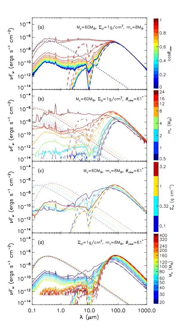

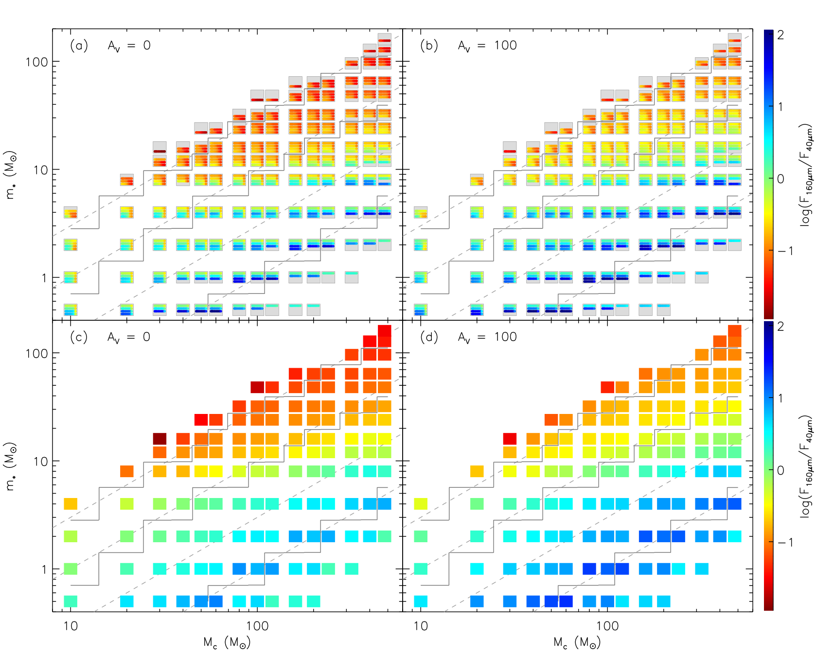

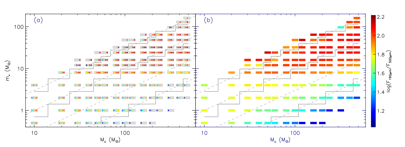

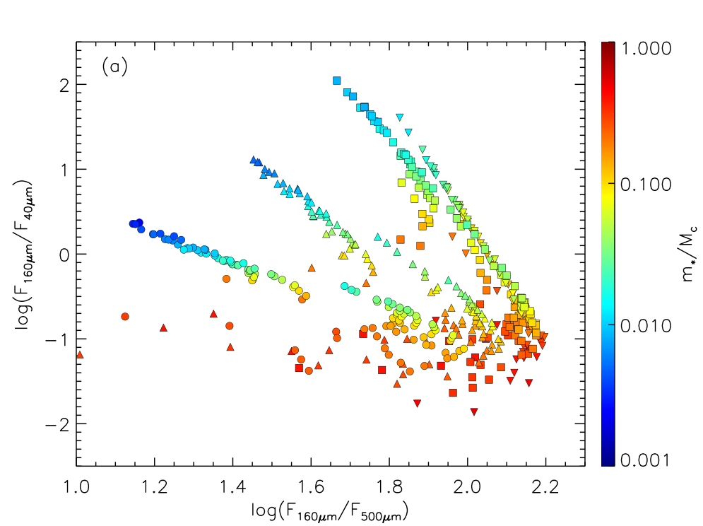

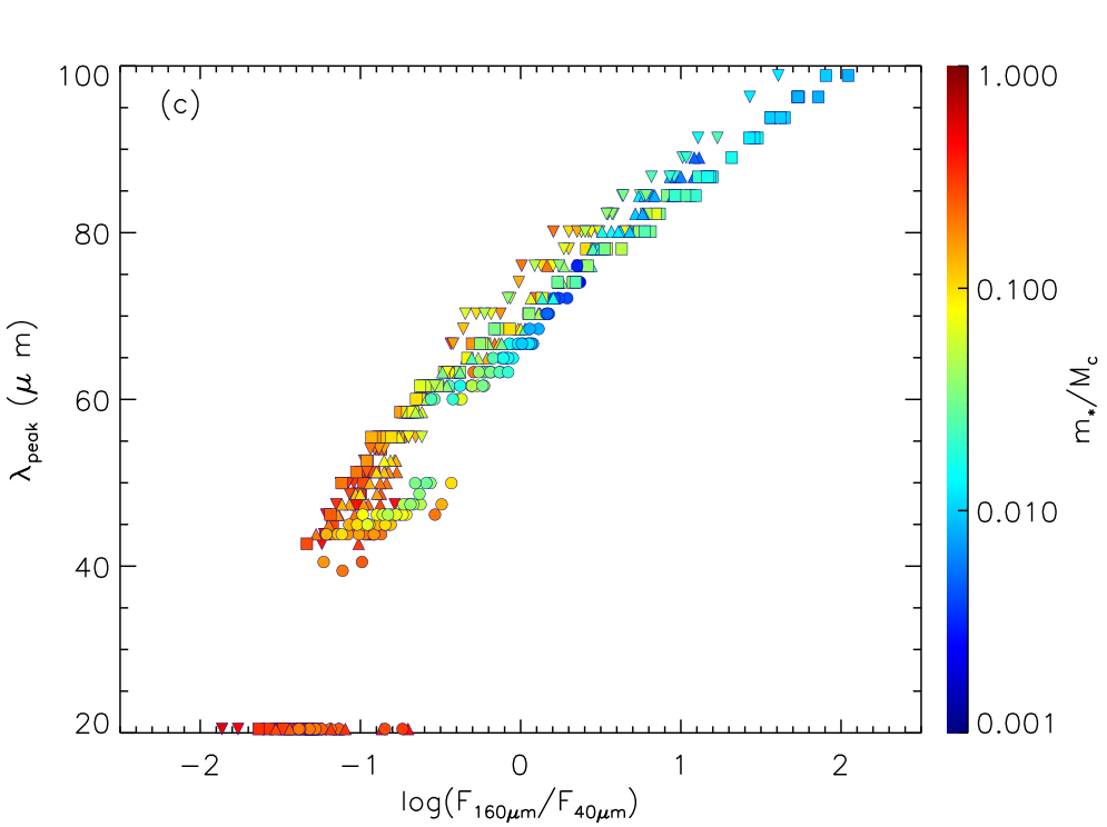
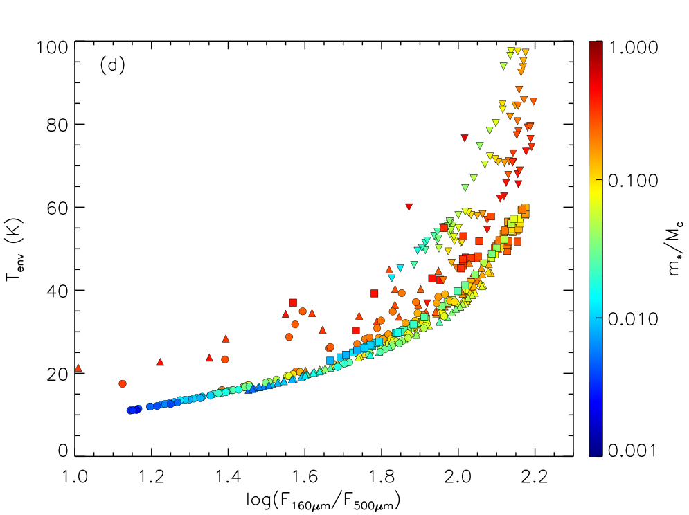
Figure 5 shows example SEDs from the model grid. From top to bottom, the four panels show how the SED is affected by the viewing inclination angle , growth of the protostellar mass , the mass surface density of the star-forming environment , and the initial core mass .
Panel (a) compares the SEDs of a same physical model (), but viewed at different inclination angles. From an edge-on view () to a face-on view (), the SED at shorter wavelengths increases, while the SED at wavelengths longer than about 100 m (i.e., longer than the wavelengths of the SED peak) does not change. In this particular physical model (), the opening angle of the outflow cavity is (). The SED becomes flat when the viewing inclination angle is smaller than this (i.e., when the line of sight toward the protostar goes through the outflow cavity).
Panel (b) shows how the growth of the protostar affects the SED along one evolutionary track (). A typical viewing inclination angle of is used here. As the protostar grows, the fluxes at all wavelengths increase, especially at the shorter wavelengths. This is not only because of the increase in total luminosity with the growth of protostar, but also because of the gradual opening-up of the outflow cavity. As the flux is increasing, the SED peak also moves from about m at early stages to about m at later stages. The SED becomes flat at wavelengths m once the outflow cavity becomes wider than the viewing inclination angle (the SED for ).
Panel (c) compares the SEDs of models with same and , but in environments with different . The mass surface density of the environment affects the SED in several ways. First, for these four models, the luminosity is higher in a higher mass surface density environment, which affects the height of the far-IR peak of the SED. This is true in general, especially at earlier stages when the accretion luminosity is dominant, but is affected by the detailed evolutionary histories (see Panel (e) of Figure 2). Second, the mid-IR fluxes are mainly determined by the emission from the accretion disk and also the dust inside of the outflow cavity, after being extincted by the envelope. Since the envelope extinction is lower in the low case, higher mid-IR fluxes are seen. Third, the outflow cavity develops faster with the growth of the protostar in the low case, which also makes the mid-IR fluxes higher and the far-IR peaks at a shorter wavelengths. Fourth, different protostellar evolutionary tracks cause the input stellar temperature to be significantly different among these mass surface densities. In addition, it is also worth noting that the depth of the silicate feature around 10 m is not monolithically dependent on the mass surface density. It is deepest for an intermediate mass surface density environment. This is because the silicate feature is mostly caused by the optical depth in the disk, and in the high cases, the mid-IR fluxes from the disk start to be buried by the emission from the warm envelope (see Paper II).
Panel (d) compares the SEDs of models with same and , but with different . With a more massive initial core, the protostar is more embedded, leading to a higher contrast between the far-IR SED and the shorter wavelength SED. In the figure, SEDs with a foreground extinction of , which corresponds to a mass surface density of , are also shown. The SEDs at all wavelengths shorter than about 100 m are affected.
II.3.2 Detailed Features of the SEDs
In this section, we discuss several characteristics of the SEDs and their distributions in the parameter space of the model grid. These characteristics include the wavelength of the SED peak, the bolometric temperature, the far-IR slope at wavelengths around m, and the mid-IR slope at wavelengths around m. As the results of the previous section have shown, these characteristics of the SED are directly affected by the initial conditions, evolutionary stages, and viewing inclination angles. While SED fitting works best with a fully sampled SED from MIR to FIR, these characteristics may help to constrain some of the conditions of massive protostars in circumstances where fully sampled SEDs are not available.
As shown in Figure 5, the wavelength of the SED peak in the far-IR is not very sensitive to the viewing inclination or the foreground extinction (except for face-on sources), and only sensitive to the physical conditions of the source (in our case, determined by the initial conditions , , and the protostellar mass ). Figure 6 shows the distributions of in the parameter space of the model grid. The SED becomes flat and therefore m once the opening angle is large and the line of sight toward the protostar goes through the outflow cavity. Such SEDs are also highly sensitive to the foreground extinction. Since foreground extinction is common in massive star forming regions and quite uncertain, we expect to see the situation represented in the right panels more often in real observations. For the models with viewing inclination angles larger than the opening angle of the outflow cavity, the effect of the foreground extinction on is minor. There is a weak dependence of on the mass surface density of the environment . In early stages, the high models have SED peaks at about m, while the low models have SED peaks at about m. In later stages, the high models have SED peaks at about m and the low models have SED peaks at about m, if the viewing inclination angle is larger than the opening angle of the outflow cavity. With a foreground extinction, the difference is even smaller. After averaging over inclination angles and mass surface densities of the environment (lower panels), it is evident that , with or without foreground extinction, is dependent on the evolutionary stages indicated by or , especially when the protostellar mass . At the stage of , which marks the transition from the main accretion phase to the envelope clear-up phase, is about m in the case of foreground extinction . At the stage that , is about m.
Figure 7 shows how the [160 m][40 m] color (defined as ) depends on the initial conditions, protostellar mass, and viewing inclination angle. The [160 m][40 m] color is related to , which is between these two wavelengths. In fact, the [160 m][40 m] color is easier to determine, since it does not require a well sampled SED around the peak position, although it is more affected by the inclination or the foreground extinction since the flux at m is used. However, as Figure 7 shows, the effects of inclination and possible foreground extinction on the [160 m][40 m] color are modest. The value of increases by about 1 when varying the inclination from a face-on view to an edge-on view, and increases by about 0.3 with a foreground extinction of . Overall, it changes by up to about 4 over the whole parameter space. The dependence of the [160 m][40 m] color on the mass surface density of environment is also relatively weak (the increase is by from the high mass surface density case to the low mass surface density case). It is sensitive to the evolutionary stage, indicated by or . Therefore the [160 m][40 m] color may be used as an indicator of the evolutionary stage of massive protostars, in addition to the peak position of the SED. The SEDs at the stage when have and those at the stage of have .
Besides the peak wavelength, one can also use the flux-weighted mean wavelength as an indicator of the evolutionary stage. The concept that is related to this is the bolometric temperature, which is defined as the temperature of a blackbody having the same mean frequency as the observed SED (Myers & Ladd 36), which can be written as . Here, for , we use the flux-weighted mean frequency in the wavelength range of m. This is because often only infrared data are available when constructing SEDs for massive protostars, and the fluxes at shorter wavelengths normally suffer from high levels of extinction, since massive protostars are typically highly embedded in high mass surface density clouds. Compared to the peak wavelength of the SED, the bolometric temperature is not so affected by whether the SED is well sampled around the peak. However, it is sensitive to the inclination and the foreground extinction, since the short wavelength fluxes are used to determine . Therefore one should be cautious when using the bolometric temperature to estimate the evolutionary stage, especially for individual sources. For a sample with a large number of sources, we expect the effects of different viewing inclination angles will be averaged out.
Figure 8 shows how the bolometric temperatures are affected by the initial conditions, the evolutionary stages, the viewing inclination angles, and foreground extinction. From Panel (a) and (b), we can see that is distinctively different for the inclinations at which the line-of-sight toward the central protostar goes through the outflow cavity, compared to those at which the line-of-sight goes through the envelope. In the former case (low inclination angles), is K without foreground extinction, and about 200 K if a foreground extinction of is applied. In the latter case (high inclination angles), is less affected by the foreground extinction. ranges from about 30 K to about 120 K without foreground extinction, and up to about 80 K with a foreground extinction of . is slightly dependent on the mass surface density of the environment , which makes increase by about 30 K from the highest to the lowest in the case without any foreground extinction, which will lower the effect. At a typical inclination of and averaging over the mass surface density of the environment, the bolometric temperature is sensitive to the evolutionary stage indicated by or , i.e., how embedded the protostar is, as Panels (c) and (d) show. At the stage where (which corresponds to the transition from Class 0 to I in low-mass star formation), K in the case of no foreground extinction, and K with a foreground extinction of . These values are higher than K, which is commonly used as the boundary between the Class 0 and Class I sources in low-mass star formation studies (Chen et al. 13). However, in the cases of low and low , which is closer to the situation of normal low-mass star formation, this transition does occur at about K.
Figure 9 shows the far-IR/sub-mm slope of the SED defined by in the parameter space. As Figure 5 has shown, the slope in this wavelength range is not affected by the inclination or foreground extinction, therefore we only consider its dependence on , and . As Figure 9 shows, the far-IR slope of the SED has a clear dependence on the protostellar mass. As the protostar grows, the far-IR slope becomes steeper, which can be also seen in Panel (b) of Figure 5. Unlike the peak wavelength or colors of other wavelength ranges discussed above, the far-IR slope has only a weak dependence on the initial core mass (or the current envelope mass), especially when the protostellar mass . The mass surface density of the environment also affects the far-IR slope of the SED. In a high mass surface density environment, the higher column density of the envelope causes more shorter wavelength emission from the inner hot regions, such as disk or innermost envelope, to be shifted to longer wavelengths, leading to a steeper slope of the far-IR/sub-mm SED. Although the far-IR slope of the SED is not so affected by the viewing inclination angle or the foreground extinction, and thus is mostly only dependent on the physical conditions of the source, in real observations, it is affected by the ambient clump material, which is not included in our models. Also the exact value of the slope is affected by dust emissivity properties.
Figure 10 shows the slope of the SED from 20 to 40 m in the parameter space. The SED slope at this wavelength range can be significantly affected by the mass surface density of the environment, , from a relatively flat slope with to a steep slope with , given with the same initial core mass and protostellar mass. This is caused by the significant effects of the column density of the envelope on the fluxes around m which is mainly from the disk, dust inside of the outflow cavity, or the innermost hot envelope. After averaging over , one can clearly see that the SED slope at 20 to 40 m depends on the evolutionary stages indicated by or , i.e., how embedded the protostar is, rather than simply on , i.e., the growth of the protostar. The SED slope at this wavelength range is also affected by the viewing inclination angle, but normally within a range of about one order of magnitude, not considering the extreme cases such as a face-on source. The foreground extinction has a modest effect on the slope compared with that due to the evolution, changing by about 0.6 for a foreground extinction of .
Figure 11 shows how the SED features discussed in this section, including the [160 m][500 m] color, [160 m][40 m] color, [40 m][20 m] color, and the SED peak wavelength correlate to each other. As discussed above, all these colors at different wavelength ranges can be used to estimate the evolutionary stages, but they are sensitive to different components of the source. The [160 m][500 m] color is mostly affected by the envelope, while the [160 m][40 m] or [40 m][20 m] colors are more sensitive to the inner warmer regions, including the outflow cavity wall. Panel (a) and (b) clearly show that the long-wavelength color and the short wavelength colors correlate to each other, but the correlations are affected by the initial condition of the source, especially the environmental mass surface density . Panel (c) shows that the [160 m][40 m] color is well correlated with the peak wavelength of the SED, except for some models at late stages or very wide outflow opening angles, for which the SED peaks are at wavelengths m. As mentioned above, both of these two features can be used to indicate the evolutionary stages, but the [160 m][40 m] color is easier to determine since it does not require a well sampled SED around its peak position.
II.3.3 Flashlight Effect
As discussed above, the observed SED is highly dependent on the viewing inclination angle, because the existence of the low-density outflow cavity allows more radiation to escape from the polar direction, which is known as the “flashlight effect”. This causes the bolometric luminosity integrated from the observed SED to deviate from the true bolometric luminosity of the source by a factor which depends on the inclination. Panel (a) of Figure 12 shows the ratios between the bolometric luminosities inferred from SEDs by assuming isotropic radiation, , and the true bolometric luminosities, , in the model grid. As the figure shows, the degree of the flashlight effect is almost completely dependent on two factors: the opening angle of the outflow cavity, , and the viewing inclination angle, . In most of the cases where , will overestimate by a factor up to 10, while in most of the cases where , will underestimate the true luminosity . For an opening angle of about , the inferred luminosity overestimates the true luminosity by a factor of for a face-on view and underestimates the true luminosity by a factor of 10 for an edge-on view. For an opening angle of about or smaller, the inferred luminosity is close to the true luminosity for most inclinations, except at a face-on view.
In real observations, the luminosity directly inferred from the SED further deviates from the true luminosity due to possible foreground extinction. Panel (b) of Figure 12 shows the ratios between the luminosities inferred from SEDs with and the true bolometric luminosities of the sources. In such a case, most of the inferred luminosities are underestimating the true luminosities. Since the foreground extinction mainly lowers the SEDs at shorter wavelengths, which mainly affects the SEDs at lower viewing inclination angles, the flashlight effect is not so much affected by the foreground extinction, if the inclination angle is larger than the opening angle of the outflow cavity. In this case, the flashlight effect is significantly affected by the opening angle of the outflow cavity, but only very weakly affected by the inclination angle. With a foreground extinction of , for an opening angle of about , the inferred luminosity underestimates the true luminosity by a factor of about 10, no matter the viewing inclination angle.

II.3.4 Temperature Evolution in the Envelope

The radiative transfer simulation also predicts the dust temperature profiles for the models in the grid. Panel (a) of Figure 13 shows the evolutions of the mass-weighted mean temperature in the whole envelope as a function of protostellar mass under different initial conditions. The envelope temperature has a clear dependence on the protostellar mass and the mass surface density of the star-forming environment, , but only a weak dependence on the initial core mass, . In the low mass surface density cases ( and ), at early stages, the core has a mean temperature of K, while with , the mean temperature is about 30 K, and in the high mass surface density case, the temperature reaches about 50 K, even in the earliest stages. As the protostar grows, the envelope becomes warmer. There is a significant increase in the envelope temperature around . The peak temperature is reached at . The peak temperature of the high mass surface density core is about 100 K. The mass surface density of the star-forming environment affects the temperature in the envelope in several ways. As discussed in §II.1, in a high mass surface density environment, the core is more compact and collapses with a higher accretion rate, leading to a higher luminosity. The high luminosity and the small size of the core combined make the temperature higher in such a core. In some models, the temperature starts to decrease in the final stages. This is because of the wide opening angle of the outflow cavity starts to suppress the heating from the protostar due to escape of radiation through the low-density outflow cavity.
The different luminosities and envelope densities in the various environments have a more significant impact on the temperature in the innermost region of the envelope. Panel (b) shows the mass-weighted mean temperature in the region of the envelope within 1000 AU from the protostar. On this scale, the peak temperature of the high mass surface density core can reach about K at around . For most of the models in low mass surface density environments ( or ), the mean envelope temperature on the 1000 AU scale is below 100 K in early stages () and below about 200 K in later stages.
Hot core chemistry is initiated when the temperature reaches about 100 K, at which point dust grain ice mantles are largely sublimated and various complex molecules are released to the gas phase, producing important observational diagnostics for the protostellar stage of massive star formation. Panel (c) of Figure 13 shows the evolution of the hot core size (defined as the size of the envelope that has a mass-weighted mean temperature of 100 K) with the growth of the protostar under different initial conditions. In the early stages, the hot core region is only present within a small zone of several hundreds of AU. Later on, when , the hot core is typically of a scale of several thousands of AU. In addition, the size of the hot core has clear dependence on the mass surface density of the environment in the early stages. However, this dependence becomes weaker in the later stages, when the hot core is fully developed. The dependence of the envelope temperature on the mass surface density of the environment suggests that even for protostellar cores with the same mass and at the same evolutionary stages, the chemistry can be significantly affected by the star-forming environment, which is not only true for massive protostars, but also for the low-mass protostars forming alongside them (Zhang & Tan 56).
For prestellar core or early-stage protostellar cores, grey-body fitting is often performed to estimate the temperature of the cores (e.g., Elia et al. 19). Figure 14 shows how the mean mass-weighted temperature in the envelope differs from the grey-body fitted temperature in our model grid. Here the grey-body temperature is obtained by fitting the model fluxes at 100, 160, 250, 350, 500, and 850 m following the greybody spectrum , where the dust emissivity index is set to be 2 and is the Planck function. The fitting gives higher for later-stage protostellar sources, which are not shown in this figure. For the models with , the mean temperature in the envelope is always K, as shown above. The greybody temperature is always higher than and as the source evolves, it soon increases from about 20 K to 100 K. In the case of , the greybody temperature follows better in the early stages. We note that our model grid only covers the protostellar phase of massive star formation when a protostar has formed, while the grey-body fit works best for the prestellar phase or early protostellar phase.
Panel (d) of Figure 11 shows how the mean temperature in the envelope correlates with the [160 m][500 m] color. These two properties are well correlated, especially for models with and at evolutionary stages with . This correlation, taking into account the correlation between and , is consistent with that found by Elia et al. [19] from a large sample of cores/clumps observed in the Hi-GAL survey. Their results extend this correlation further to even earlier stages with K, which is not covered by our model grid.
II.4 Caveats of the Model Grid
Here we describe several important caveats and limitations of our SED model grid. First, the model grid is based on the Turbulent Core model of McKee & Tan [33], in which massive cores are embedded in a larger ambient clump that will form the star cluster. The cores are assumed to be in pressure equilibrium with the ambient clump, and the surface pressure on the core is characterized using the mean mass surface density of the clump , which is why is used as one of the primary parameters of the model grid. However, except via this parameter, the clump itself is not included in the radiative transfer simulations, which is not realistic. We ignore the ambient material because it would bring in more free parameters about the sizes and density distributions of the clumps, which are highly uncertain. The ambient clump may affect the SEDs in two ways. First, it provides additional foreground extinction to lower the fluxes at shorter wavelengths. Second, it provides additional emission at longer wavelengths. The former effect can be compensated by the free parameter of foreground extinction , but the latter effect is not taken into account in our model grid. Therefore, an aperture should be carefully chosen at wavelengths m to exclude the contribution of the ambient clump material in deriving the fluxes at these wavelengths before performing the SED fitting, i.e., the model grid fitting should be done on clump-envelope-background-subtracted SEDs.
Second, in the current model grid, when constructing the SEDs, we have summed up all the photons emitted in a specified direction, no matter from where they emerge. That is to say, we are not applying any aperture to exclude the emission from any part of the model core, i.e., these are total SEDs, including from parts of the outflow that extend beyond the core. However, observations of real sources at different wavelengths by different instruments may be on different scales, which also need to be considered when performing the SED fitting.
Third, the observed short wavelength fluxes at m are affected by PAH emission and thermal emission from very small grains that are transiently heated by single photons, and these effects have not been included in our radiative transfer models. Therefore we expect the models are under-predicting the real fluxes at these wavelengths. In the example we show in §IV, we set the observed fluxes at m to be upper limits. However, users can freely adjust which data points should be used as limits according to their situation and needs, and the fitting program provides high flexibility for setting the upper/lower limits and uncertainties (see §III).
Finally, some detailed features of the SEDs, such as the peak wavelength and the long wavelength spectral index, may be affected by the particular dust models used in the radiative transfer simulations. Although the general trends of these features with the initial/environmental conditions () and evolution () discussed above should not change, the exact values may be affected.
III SED Fitting
We use minimization to find the best model to fit the observed SED. Assuming that we have observed flux densities with upper and lower uncertainties of and at wavelengths , and for each model (i.e., each set of , , , , , ) we have model flux densities (see Equation 3) at these wavelengths, the reduced is defined as
| (4) | |||||
where , and are derived from , , and (see §III.1). For used as upper limits, , i.e., no contribution to the if , and for used as lower limits, , i.e., no contribution to the if . The total number of data points contains both normal data points and upper/lower limits.
During each fitting, we first search for a minimum by varying the foreground extinction for each set of . We then compare these minimum values to find the best models in the 5 dimensional parameter space formed by different (4 dimensions if an exact source distance is provided). We also select another group of best models. For each set of , we search for the minimum by varying , , and , and then compare these minimum values to find the best models in the 3 dimensional parameter space formed by different . Therefore, each member in this group of best models is a different physical model. In the released code, both groups are output and users can choose which to use according to their need.
While the defined in Equation 4 is used in the ranking and selection of the best fitted models, we also define
| (5) |
where is the number of data points that have non-zero contributions to . Note that for the same observed SED, is dependent on the model SEDs. For example, for a data point used as an upper limit, if the model SED is higher than that data point, it is counted in , while if the model SED is lower than that data point, it is not counted in , since it is not contributing to . Therefore is the average deviation of the model SED from the constraining data points.
The SED fitting tool as well as the model grid are available for download. 11 1 See https://doi.org/10.5281/zenodo.1045606 (catalog https://doi.org/10.5281/zenodo.1045606). Currently, the fitting tool is written in IDL, therefore the IDL software needs to be installed before running the fitting program. However, knowledge of the IDL language is not necessary. An instruction file including detailed information about the structure of the package, its installation, editing input parameters, running the fitting program, and output files and figures are included in the package. In Section IV, we will show an example of the SED fitting (the same example is also included in the package) and discuss the output results and figures. Currently, the fitting program is designed to fit SEDs of individual sources, However, it can be easily adapted to perform recursive fitting to a sample of SEDs. It takes about 1 minute to fit an SED running the program on the processor of a typical current laptop or desktop computer.
III.1 Treatment of the Errors
The fitting is performed in logarithmic space since the fluxes are nonlinear with wavelength and most of the errors are best described as certain percentages of the fluxes. Assuming the observed flux and its error at a certain wavelength are and , i.e., and , the expectation and variance of the fluxes in logarithmic space are related to these values by
| (6) | |||||
and
| (7) | |||||
This is only valid when the percentage errors are small, since it is a first-order approximation. In real observations, due to the uncertainties in brightness calibration, background subtraction, and selection of apertures to integrate the emission, the percentage uncertainties in the observed flux can easily be several or higher, in which case the error becomes asymmetric around the observed flux in the logarithmic space. Therefore we define the following fluxes and errors in logarithmic space:
| (8) |
| (9) |
| (10) |
which are simply obtained by converting the data points and error bars to logarithmic space. The log space flux densities and errors in these two methods start to differ significantly when the percentage error becomes . We allow both types of conversion in the fitting program. If the first method is used, the input upper and lower errors need to be same, while if the second method is used, the users can input different upper and lower errors for each flux. We use the second method in the example discussed in §IV.
In the second method, the data points with lower errors larger than 100% have log space that is infinite, and therefore act as upper limits and have no constraints on the models below the observed fluxes. Therefore we provide a third option so that certain constraints can still be applied to the models even in such a situation. If at some wavelength , we set . However, unlike the normal data points, the contribution of this data point to the total is set to be , where , instead of . The reason to choose such a function is that when is small and when is large, so that unlike a data point with that has no constraint on the model SED, it still tends to select the models with fluxes closer to , but the constraint is not as strong as a normal data point with , since the contribution to the increases with in a logarithmic form. This method thus tends to select models that are themselves upper limits of the range of possibilities.
To sum up, when the errors of the observed fluxes are small and symmetric, or the measurements and errors are statistically well defined, the first option may be used. Otherwise the second option should be used. The third option provides a special treatment for the data points with 100% lower errors. In the fitting program, different options can be assigned to different data points.
Here we emphasize that the value we define here is not statistically meaningful, especially given the assumption of normally distributed errors, since in the more general case it is then not linked to a well-defined probability. Often we expect errors to be dominated by uncertain systematic effects, such as clump background subtraction. Thus the method presented here only provides a way to compare different models in the model grid to select the ones that are close to the given observed data. That is to say, our focus is comparing the values of models in one SED fitting, not on the absolute values, nor on comparing the values of fittings to different observations.
IV G35.20-0.74 as an Example of SED Fitting
IV.1 Model Parameters and Degeneracies
| Model | |||||||||||||
|---|---|---|---|---|---|---|---|---|---|---|---|---|---|
| () | () | () | (∘) | (kpc) | (mag) | (AU) | (∘) | () | () | () | |||
| 1 | 2.64 | 3.12 | 480 | 0.1 | 16 | 48 | 2.2 | 42 | 15 | ||||
| 2 | 2.70 | 3.90 | 100 | 3.16 | 12 | 34 | 2.2 | 26 | 20 | ||||
| 3 | 2.84 | 3.35 | 200 | 0.316 | 12 | 22 | 2.2 | 45 | 17 | ||||
| 4 | 2.90 | 3.43 | 320 | 0.1 | 24 | 68 | 2.2 | 82 | 27 | ||||
| 5 | 3.12 | 3.69 | 400 | 0.1 | 16 | 58 | 2.2 | 38 | 17 |
Notes:
a The primary parameters.
b The additional independent parameters.
c Fixed in this example.
d Selected derived secondary parameters.
We use the SED of the massive protostar G35.20-0.74 as an example for demonstrating the SED fitting program with our model grid. The SED is constructed based on the SOFIA-FORCAST observations from 20 to 40 m, along with fluxes measured at other wavelengths from 3.6 m to 500 m using archived data of other instruments, including Spitzer-IRAC, Herschel-PACS/SPIRE, and other ground-based infrared instruments. The SOFIA observation of this source is part of the SOFIA Massive Star Formation (SOMA) survey (De Buizer et al. 15). The SOFIA continuum images and SEDs of this source were first presented and analyzed by Zhang et al. [57], with the then-under-development model grid and a limited, ad hoc exploration of parameter space. Later, the method used to derive the SED from the continuum imaging was improved by De Buizer et al. [15]. In that paper, the current model grid was used to fit the SED of G35.20-0.74 and seven other massive protostars, but without detailed discussion about the fitting process and the full results. Here we focus on using this SED as an example to demonstrate the SED fitting program. The values of the fluxes and their errors are listed in De Buizer et al. [15]. For the details about the observations and derivation of the SED, please also refer to De Buizer et al. [15]. Also, following De Buizer et al. [15], in the example here, we set the short wavelength fluxes at m to be upper limits, as discussed in §II.4.
As described in the previous section, the fitting program produces two groups of best models. The first group contains models which are different in the five dimensional parameter space comprised of , , , and (four dimensional parameter space if the exact value of is provided). The second group further selects the best models that are different in the three dimensional space comprised of the three primary parameters , , . Therefore the best models in the first group may share the same physical model but differ only because of different distances or viewing inclinations, while in the second group the models are actually different in their initial conditions or evolutionary stages, and have different physical structure and properties. Figure 15 shows all the model SEDs with in the two groups of results. Here the distance to the source is set to be a fixed value of 2.2 kpc (Zhang et al. 54; Wu et al. 53). In this case, the best fit model has . In the first group of results (upper panel), there are 171 model SEDs with , 670 model SEDs with , and 2441 model SEDs with , among the total 8640 model SEDs. In the second group of results (lower panel), there are 27 models with , 80 models with , and 178 models with , among the total 432 model SEDs. For the relatively well-fitted models with , on average, a change of 0.3 in will not affect the rank of the models determined by the primary parameters of , and . We can consider in the space to be the fitting uncertainty of the inclination in this case. But as we will show below, this is actually dependent on the exact model.
As discussed in the previous section, in our fitting, the upper limits work as a normal data points and contribute to if the model SED is higher than the upper limits. Therefore, it is possible that the best models are above one or more upper limits, which is the case shown here. However, users can assign smaller errors to the upper limits to make them stronger constraints. In fact, very small errors for the upper limits practically exclude models with fluxes above the upper limits. It is also worth noting that, in this example, the group of best models also appear to under-predict the fluxes at longer wavelengths m. Among the 7 sources whose SEDs were fitted with our model grid by De Buizer et al. [15] (8 sources were fitted in this paper, but one source is without fluxes at wavelengths m; see also Section IV.3), two sources (including G35.2-0.74) show such deviation at the long wavelengths. Since the slope at wavelengths m of the model SEDs are similar to the observed slopes, the adopted dust models are not likely to be the reason for such deviation. It is more likely caused by the inclusion of additional clump material at these long wavelengths when deriving the SEDs from observations.


Figure 16 shows how the models deviate from the observed fluxes and colors (i.e., SED slopes) at different wavelengths. Only the models in the second group of results are shown. The best five models are also marked. Most of the models with (), which corresponds to an average deviation of at each data point, are indeed located within the range of at the wavelengths shown here, suggesting the data points of different wavelengths are evenly contributing to the , and the fitting is constrained over the whole range of wavelengths. The fitting is especially well constrained in the wavelength range of m in terms of the absolute fluxes and also the SED slope. The best models are under-predicting the m flux at levels of about , and also under-predicting the m flux at levels of about . In addition, most of the models are predicting a slightly steeper slope between 160 and 500 m at levels within . At short wavelengths, although the data points at m are set to be upper limits, most of the best fitted models are still close to the data points.
Table 1 lists the parameters of the five best models in the second group of results which are different in the primary parameter space of (, , ). The additional independent parameters (, and ) to achieve these minimum are also listed. We also list several important parameters that are derived from the primary parameters based on the physical model, including: the core radius , which in the model only depends on the initial conditions and and is constant over time; the opening angle of the outflow cavity ; the current envelope mass ; the accretion rate from disk to protostar ; and the total luminosity . Note that is different from the value directly integrated from the SED due to the effect of inclination (i.e., the flashlight effect) and foreground extinction. Besides the used to rank the models, is also listed, showing the average deviation between the model SEDs and the observed data points. Note these results are slightly different (slight change of ordering of the best models) from those shown by De Buizer et al. [15]. This is because here we have improved the quality of the model SEDs by using larger number of photon packets in the Monte-Carlo RT simulations and reducing the Monte-Carlo noise levels of the model SEDs. The improvement of the model SED qualities slightly affects the fitting especially at short-wavelengths for more embedded or more edge-on sources. Among the best five models, the initial core mass is constrained to be (most likely ) and the protostellar mass is constrained to be . The half opening angle of the outflow cavity is constrained to be , the accretion rate is constrained to be between to (most likely ), and the total luminosity is about . On the other hand, the clump environment mass surface density and the inclination angle are not well constrained.
For these five best models, Figure 17 shows how the inclination would change the fitting when other parameters are kept the same. Note that a different foreground extinction, , is adopted to minimize the for each inclination angle. For three of the five models (Models 1, 4 and 5 shown in the first, fourth and fifth rows; see also Table 1), the fitting results are not so sensitive to inclination, except close to , i.e., a face-on view. In this case the inclination is not well constrained. On the other hand, in the other two models (Models 2 and 3), the fitting results are highly sensitive to the inclination angle. The reason for this difference is that in the former case, the unextincted SEDs of different inclinations are all above the observed data points at wavelengths m, and by adjusting foreground extinction , the model SEDs of different inclinations except close to a face-on view can all have relatively good fits to the observations. In the latter case, the unextincted model SEDs of higher inclinations are below the observed fluxes and the fitting cannot be improved by adjusting , therefore relatively good fitting can be achieved only at a narrow range of inclinations. This suggests a certain degeneracy between the inclination and foreground extinction .
Figure 18 shows the distribution of the models in the primary parameter space comprised of , , and . The first row shows the distribution of of the best models in the space in the first panel, and the distributions of , , to achieve these best models in the second to fourth panels. Similarly, the second row shows the distribution of of the best models in the space and the corresponding distributions of , and , and the third row shows the equivalent distributions in the space. In the space, the models with (inside the red contour) occupy a region with high but spanning the full range of (first row, first panel). For these models, the initial core mass appears to be higher in a lower surface density environment. The range of of the best models () gradually increases from at to at . The models are more constrained in (e.g., second row, first panel). All of the best models () have higher than about 10 and mostly have , but extend to higher for the models with in the range of . The fitted inclinations are mostly around , i.e., between the line of sight and the outflow axis, for the best models with and (e.g., first row, third panel). For the best models with low () and high (), is in the range of about . For most of these best models, a foreground extinction of mag is needed to achieve the minimum (e.g., first row, fourth panel). To summarize, in the example shown here, while and are relatively well constrained, is not. However if the inclination can be independently determined from other observations such as those of outflow kinematics, then this degeneracy can be further broken.
Figure 19 shows the distribution of all the second group models (different in the space) with with various secondary parameters. In the model grid, while all the SEDs are determined by the three primary parameters , , and , along with the additional independent parameters , and , the secondary parameters, which are derived from the primary parameters and describing the properties of the protostar, envelope, outflow cavity and disk, are of more interest in understanding the physical conditions of the observed massive protostars. Panels (a) and (b) show the distribution of the models in the and diagrams. As discussed in previous sections, the location in the diagram and the parameter are often used as indicators of the evolutionary stage. Most of the models with are located between and 1, which corresponds to the turning points of the evolutionary tracks in the diagram (see Figure 4), and the best models that have (red and orange colors) are located around . This suggests that this source is still highly embedded and in the main accretion phase.
Panels (c), (d) and (e) show the relation of the total luminosity , accretion rate , and age since the start of star formation, with the protostellar mass in the fitted models. These relations are determined by the evolutionary models (see Figure 2). The total luminosity is highly dependent on the protostellar mass and not so much on the other primary parameters. Since is relatively well constrained as discussed above, the total luminosity is also constrained well. The best models with have a luminosity from several to . The accretion rates of the models with are constrained to be , and the protostellar age from several to several yr. They are affected by the environmental mass surface density , which is less well constrained in this case.
Panel (f) shows the relation between the inclination and the opening angle of the outflow cavity of the fitted models. All the models have an inclination angle larger than the outflow cavity opening angle, i.e., the line of sight toward the protostar goes through the envelope. As discussed above, the inclination angle is not well constrained in this case, but interestingly, for the models with , the opening angles are either close to the inclination angle up to about 40∘ or around , despite the wide range of inclinations. All the best five models have opening angles around .
Panel (g) shows the distribution of the fitted models in the space of the two additional independent parameters and . The models with have mag, with most of them within 100 mag. Panel (h) further compares the fitted with the values that correspond to the mean mass surface densities of the ambient clumps . On average, the contribution of the ambient clump to the foreground extinction to the core should correspond to , which we define as . But the foreground extinction in the real situation will differ from due to clumpy and/or anisotropic structures in the ambient clump, and additional foreground extinction which is not related to the host star-forming clouds. For the best fitted models which have , with , the fitted is within , but for models with , the fitted can be as high as , which indicates that the foreground extinction needed to fit the observed SED may not be only that expected from the ambient clump. Thus, if a constraint is imposed that the foreground extinction should be no more than that expected given the value of , then some low models would be excluded in this case.
Panels (i) and (j) compare the fitted total luminosities, , with , the bolometric luminosities directly integrated from the observed SED (see also Figure 12). The latter luminosity is also slightly dependent on the model fitting because of the uncertainties of the SED at the wavelength ranges not covered by the observation. For the models with , is in the range of . This is caused by a combined effect of the inclination (flashlight effect) and the foreground extinction (see §II.3.3). According to Figure 12, such a ratio between and is consistent with an outflow opening angle of about .
In the end, we note that the above discussion is based on a specific example and may not be general (see §IV.3). However, during each fitting, in addition to giving just a few best models, the program will generate similar figures to help the users to better understand the results. The above discussion serves as an example of what information we can expect from these figures.
IV.2 Discussion of the Source
G35.20-0.74 is a massive protostar in a broader region of star formation located at a distance of 2.2 kpc (Zhang et al. 54; Wu et al. 53). CO(1-0) and (2-1) observations have revealed a wide outflow structure in the direction of northeast-southwest which extends to from the central source (Gibb et al. 20; Birks et al. 7). Perpendicular to this, CS(2-1) observations have revealed a ridge-like structure (Dent et al. 16), which has been further resolved into a -long filament with a string of cores embedded by ALMA (Sánchez-Monge et al. 43, Sánchez-Monge et al. 42) and SMA (Qiu et al. 39) in the sub-mm continuum. Heaton & Little [22] observed this source in centimeter radio continuum and were able to resolve three compact sources arranged north-south, and concluded that the central source was likely an UCHII region, while the north and south sources had spectral indices consistent with free-free emission from a collimated, ionized, bipolar jet. Since then it has been debated whether the NE-SW CO outflow is caused by the ionized jet undergoing precession, or if they are composed of separate outflows driven by different sources. This elongated radio continuum emission was further resolved into 17 individual knots lying along the N-S direction by the VLA (Beltrán et al. 5; Gibb et al. 20), with the driving source identified as an UC/HCHII region. This radio source is coincident with one of the embedded cores identified in sub-mm observations (Core B identified by Sánchez-Monge et al. 43, Sánchez-Monge et al. 42 and MM1b identified by Qiu et al. 39). The N-S outflow is also seen in NIR and MIR observations (Dent et al. 17; De Buizer 14). At these wavelengths, the emission is elongated in the N-S direction but peaked to the north of the identified radio source and continuum core. It has been argued that the outflow/jet is blue-shifted to the north and the emissions at NIR and MIR are dominated by the northern near-facing outflow cavity. However, at longer wavelengths of m, the SOFIA-FORCAST observations have revealed the southern, far-facing outflow cavity (Zhang et al. 57).
In our previous fitting of the SED of this source (Zhang et al. 57) with an earlier version of our radiative transfer models (which had fixed outflow cavity-opening angles) and using a limited, ad hoc exploration of model parameter space, this source was estimated to be a protostar with , accreting at rates of . The total luminosity was estimated to be , and the opening angle of the outflow cavity was estimated to be . Compared with these earlier results, our completed model grid and SED fitting program presented in this paper have estimated a protostellar mass of and a total luminosity of . Sánchez-Monge et al. [43] has identified a Keplerian disk in Core B with rotation corresponding to a central mass of , and they argued that the disk is around a binary based on the total luminosity. Indeed, a binary system of UC/HCHII regions is seen by Beltrán et al. [5] at the position of Core B. Our model is based on a single protostar, which under-predicts the total protostellar mass if the luminosity is from a binary, therefore our new estimation is quite consistent with the mass estimation from gas kinematics. Compared with the previous estimation, our new estimation of the opening angle of the outflow () is also more consistent with the MIR observations which suggests a narrow outflow cavity (e.g., De Buizer 14).
Our SED fitting also estimates the current envelope mass to be about , and a ratio between the protostellar mass to envelope mass of . The total mass of the filament has been estimated to be about 160 and the mass of the core that hosts the driving source of the N-S outflow/jet was estimated to be about 18 (Qiu et al. 39). However, these masses are concentrated to the fragments with sizes of about , and the MIR emission shows that there is a narrow outflow cavity existing on a scale of about , suggesting envelope material extends at least to such a scale. This indicates that the total mass of the gas envelope surrounding this N-S outflow should be higher than 160 , which is consistent with our estimation of the current envelope mass. However, unlike our model which has a highly idealized spherical core with smooth density distribution, the observations show that the envelope is actually highly fragmented and may be feeding several protostars and close binary systems. Therefore, if one of the protostars or close binary systems is contributing most of the IR emission (e.g., Core B in this case), our model grid is still able to generate relatively accurate estimates about this main source and overall properties of the large envelope. However, due to the fragmentation, the mass reservoir for each protostar or close binary system is smaller than what the model suggests and therefore the sources may be at a later evolutionary stage than indicated in the models.
We note also that our previous model fitting of G35.20-0.74 [57] used not only the SED, but also the MIR to FIR flux intensity profiles along the outflow axis. In a follow-up paper, we plan to extend our presented model grid to include multiwavelength images, which can be used in such ways to further constrain the protostellar properties.
IV.3 Standard Format Output for SOMA Survey Protostars
Finally, to illustrate simplified outputs from the SED fitting tool, in Figure 20 we show a standard format output of 3 panels, i.e., vs. , vs. , and vs. , which were already presented in Figure 18. These results are shown for G35.20-0.74, and also for seven other massive protostars from the first SOFIA Massive (SOMA) Star Formation survey data release (De Buizer et al. 15). We do not discuss these other sources individually in detail here, but these results complement the simpler SED fitting results (i.e., the lists of the top 5 SED models) for these sources presented by De Buizer et al. 15 and the discussion of these sources in this paper.
Concerning general trends, from Figure 20 we see that among the three primary parameters, the protostellar mass is best constrained. Most of the sources have around . But in G45.47+0.05 is clearly higher around and in IRAS 07299, is slightly lower (around ). In the space, for all the sources, the best models (, within the red contours) occupy a region with lower at higher and higher at lower , similar to what we found in G35.20-0.74 in the previous sections. But there is a clear difference in the ranges of of the best models from source to source, with G45.47-0+0.05 having highest and AFGL4029 having relatively low . As discussed above is least constrained, with most of the sources having best models spanning over the full range of in the model grid. The constraint of is slightly better in IRAS 20126 and IRAS 07299 in which the best models concentrate in , and G45.47+0.05, where the best models concentrate in .
V Discussion and Conclusions
We have presented a model grid for fitting the SEDs of massive protostars. The model grid is based on the Turbulent Core model of massive star formation (McKee & Tan 32, McKee & Tan 33). The initial conditions of the model grid are pressurized, dense, massive cores embedded in high mass surface density “clump” environments. These initial conditions are parameterized by the initial mass of the core, , and the mean mass surface density of the clump, . Using analytical and semi-analytical solutions, we self-consistently calculate the properties and evolutions of the rotating collapsing core, the accretion disk, the protostar, the disk wind that gradually opens up the outflow cavity, from different sets of initial conditions. The model grid covers a parameter space with and , which is consistent with the observed environments of massive star formation, and by sampling at different protostellar masses, , there are in total 432 different physical models in the current model grid. SEDs are generated via Monte-Carlo radiative transfer simulation at 20 inclinations between an edge-on view and a face-on view for each of these models, making a total of 8640 SEDs in the model grid. These model SEDs, also allowing for foreground extinction, are used to fit the observed SED via minimization.
In such a model grid, the properties and evolutions of the protostar and its surrounding structures are more physically connected, which reduces the dimensionality of the parameter spaces and the total number of models. It also helps to rule out possible fitting results that are physically unrealistic or that are not internally self-consistent. Therefore, this model grid serves not only as a fitting tool to estimate properties of massive protostars from observed SEDs, but also as a test of core accretion theory. Its use tells us whether or not the observed SEDs of various massive protostars can be explained by the core accretion theory, with different initial conditions and evolutionary stages.
We studied how the parameters , , , inclination , and foreground extinction affect the various features of the SEDs, especially the peak wavelength, the m slope, the m slope, and the bolometric temperatures. All these features show clear dependencies on the evolutionary stages. Among these features, the peak wavelength of the SED and the m slope are not so sensitive to the inclination or possible foreground extinction, except at an inclination close to face-on, while the m slope or the bolometric temperature are highly sensitive to the inclination. The environmental mass surface density, , also strongly affects the m slope, while the other features are only weakly dependent on . We found that the degree of the flashlight effect (the difference between the inferred luminosity from the SED and the true total luminosity) is almost only dependent on the viewing inclination and the opening angle of the outflow cavity. With outflow cavities with typical opening angles, the inferred luminosity can be higher or lower than the true total luminosity by a factor of a few from a low inclination to a high inclination. However, with a foreground extinction, the inferred bolometric luminosity almost always underestimates the true luminosity by a factor almost solely dependent on the outflow cavity opening angle.
We used the massive protostar G35.20-0.74 as an example of SED fitting with our model grid (see also De Buizer et al. 2017 for a less detailed application to eight sources, including G35.20-0.74). The fitting program not only provides information of a few best-fitted models, but also shows the distribution of the fitted models in the parameter space to understand constraints and degeneracies. The fitting yields a protostellar mass , a total luminosity of , an accretion rate of a few , and a half opening angle of the outflow cavity of about , which are consistent with those estimated from other observations. The fitting also yields an initial core mass of , while is not well constrained. There are certain degeneracies caused by combined effects of and . Further breaking these degeneracies will require additional observational constraints, such as using predictions of image intensity profiles (e.g., Zhang et al. 57) or radio continuum emission that traces ionized gas (e.g., Tanaka et al. 47). Compared with the widely used Robitaille et al. [40], Robitaille et al. [41] model grid (results presented by De Buizer et al. 15), our model grid yields slightly lower protostellar mass, similar total luminosities, but much higher accretion rates (accretion rates of a few are estimated using Robitaille et al. [40], Robitaille et al. [41] model). We believe that these differences are due, at least in part, to there being a wider choice of free parameters in the Robitaille et al. [40], Robitaille et al. [41] grid, which can lead to models that we consider less physically realistic, i.e., high mass infall rates in the core envelope but small disk accretion rates. Our model grid, on the other hand, is designed to include the different components more consistently with fewer free parameters, to yield results that are more physically realistic.
Future papers in this series will present the multi-wavelength imaging data, which, as mentioned, may be helpful to break model degeneracies. Extension to lower core masses is also planned (see Zhang & Tan 56 for some preliminary examples). These physical models, i.e., for the time evolution of density and temperature, are also the necessary boundary conditions for astrochemical computations and eventual line radiative transfer simulations to predict molecular line emission properties of the protostars.
References
- [1] Alves, J., Lombardi, M., Lada, C. J., 2007, A&A, 462, L17
- [2] André, P., Men’shchikov, A., Bontemps, S., et al., 2010, A&A, 518, L102
- [3] Baldeschi, A., Molinari, S., Elia, D., Pezzuto, S., Schisano, E., 2017, MNRAS, 472, 1778
- [4] Bally, J., & Zinnecker, H. 2005, AJ, 129, 2281
- [5] Beltrán, M. T., Cesaroni, R., Moscadelli, L., et al. 2016, A&A, 593, A49
- [6] Beltrán, M. T., de Wit, W. J., 2016, A&ARv, 24, 6
- [7] Birks, J. R., Fuller, G. A., Gibb, A. G. 2006, A&A, 458, 181
- [8] Blandford, R. D., Payne, D., G., 1982, MNRAS, 199, 883
- [9] Bonnell, I. A., Bate, M. R., Clarke, C. J., Pringle, J. E., 2001, MNRAS, 323, 785
- [10] Bonnell, I. A., Bate, M. R., Zinnecker, H., 1998, MNRAS, 298, 93
- [11] Butler, M. J., Tan, J. C., 2012, ApJ, 754, 5
- [12] Butler, M. J., Tan, J. C., Kainulainen, J., 2014, ApJ, 782, L30
- [13] Chen, H., Myers, P. C., Ladd, E. F., Wood, D. O. S., 1995, ApJ, 445, 377
- [14] De Buizer, J. M. 2006, ApJL, 642, L57
- [15] De Buizer, J. M., Liu, M., Tan, J. C., Zhang, Y., et al., 2017, ApJ, 843, 33
- [16] Dent, W. R. F., Little, L. T., Kaifu, N., Ohishi, M., Suzuki, S. 1985a, A&A, 146, 375
- [17] Dent, W. R. F., Little, L. T., Sato, S., Ohishi, M., Yamashita, T. 1985b, MNRAS, 217, 217
- [18] Elia, D., Schisano, E., Molinari, S., et al., 2010, A&A, 518, L97
- [19] Elia, D., Molinari, S., Schisano, E., et al., 2017, MNRAS, 471, 100
- [20] Gibb, A. G., Hoare, M. G., Little, L. T., Wright, M. C. H. 2003, MNRAS, 339, 1011
- [21] Goodman, A. A., Benson, P. J., Fuller, G. A., Myers, P. C., 1993, ApJ, 406, 528
- [22] Heaton, B. D., & Little, L. T. 1988, A&A, 195, 193
- [23] Hosokawa, T., Omukai, K., 2009, ApJ, 691, 823
- [24] Hosokawa, T., Yorke, H. W., Omukai, K., 2010, ApJ, 721, 478
- [25] König, C., Urquhart, J. S., Csengeri, T., et al., 2017, A&A, 599, 139
- [26] Königl, A., Pudritz, R. E., 2000, in Protostars and Planets IV, ed. V. Mannings (Tucson: University of Arizona Press), 759
- [27] Kratter, K. M., Matzner, C. D., Krumholz, M. R., 2008, ApJ, 681, 375
- [28] Li, J., Wang, J., Gu, Q., Zhang, Z.-Y., Zheng, X., 2012, ApJ, 745, 47
- [29] Matzner, C. D., McKee, C. F., 2000, ApJ, 545, 364
- [30] McLaughlin, D. E., Pudritz, R. E., 1996, ApJ, 469, 194
- [31] McLaughlin, D. E., Pudritz, R. E., 1997, ApJ, 476, 750
- [32] McKee, C. F., Tan, J. C., 2002, Nature, 416, 59
- [33] McKee, C. F., Tan, J. C., 2003, ApJ, 585, 850
- [34] Molinari, S., Bally, J., Glover S., et al., 2014, in Protostars and Planets VI, ed. H. Beuther et al. (Tucson, AZ: Univ. Arizona Press), 125
- [35] Molinari, S., Pezzuto, S., Cesaroni, R., Brand, J., Faustini, F., Testi, L., 2008, A&A, 481, 345
- [36] Myers, P. C. & Ladd, E. F., 1993, ApJL, 413, L47
- [37] Offner, S. S. R., Clark, P. C., Hennebelle, P. et al., 2014, in Protostars and Planets VI, ed. H. Beuther et al., 53
- [38] Palau, A., Fuente, A., Girart, J. M., et al., 2013, ApJ, 762, 120
- [39] Qiu, K., Zhang, Q., Menten, K. M., Liu, H. B., Tang, Y.-W. 2013, ApJ, 779, 182
- [40] Robitaille, T. P., Whitney, B. A., Indebetouw, R., Wood, K. Denzmore, P., 2006, ApJS, 167, 256
- [41] Robitaille, T. P., Whitney, B. A., Indebetouw, R., Wood, K., 2007, ApJS, 169, 328
- [42] Sánchez-Monge, Á., Beltrán, M. T., Cesaroni, R., et al. 2014, A&A, 569, A11
- [43] Sánchez-Monge, Á., Cesaroni, R., Beltrán, M. T., et al. 2013, A&A, 552, L10
- [44] Shakura, N. I., Sunyaev, R. A., 1973, A&A, 24, 337
- [45] Shu, F. H., 1977, ApJ, 214, 488
- [46] Tan, J. C., Beltrán, M. T., Caselli, P., et al. 2014, in Protostars and Planets VI, ed. H. Beuther et al. (Tucson, AZ: Univ. Arizona Press), 149
- [47] Tanaka, K. E. I., Tan, J. C., Zhang, Y., 2016, ApJ, 818, 1
- [48] Tanaka, K. E. I., Tan, J. C., Zhang, Y., 2017, ApJ, 835, 32
- [49] Ulrich, R. K., ApJ, 210, 377
- [50] Wang, P., Li, Z.-Y., Abel, T., Nakamura, F. 2010, ApJ, 709, 27
- [51] Whitney, B. A., Robitaille, T. P., Bjorkman, J. E., Dong, R., Wolff, M. J., Wood, K., Honor, J., 2013, ApJS, 207, 30
- [52] Whitney, B. A., Wood, K., Bjorkman, J. E., Wolff, M. J., 2003, ApJ, 591, 1049
- [53] Wu, Y. W., Sato, M., Reid, M. J., et al. 2014, A&A, 566, A17
- [54] Zhang, B., Zheng, X. W., Reid, M. J., et al. 2009, ApJ, 693, 419
- [55] Zhang, Y., Tan, J. C., 2011, ApJ, 733, 55
- [56] Zhang, Y., Tan, J. C., 2015, ApJL, 802, 15
- [57] Zhang, Y., Tan, J. C., De Buizer, J. M., et al., 2013a, ApJ, 767, 58
- [58] Zhang, Y., Tan, J. C., McKee, C. F., 2013b, ApJ, 766, 86
- [59] Zhang, Y., Tan, J. C., Hosokawa, T., 2014, ApJ, 788, 166