Fast, Accurate, and Scalable Method for
Sparse Coupled Matrix-Tensor Factorization
Abstract.
How can we capture hidden properties from a tensor and a matrix data simultaneously in a fast, accurate, and scalable way? Coupled matrix-tensor factorization (CMTF) is a major tool to extract latent factors from a tensor and matrices at once. Designing an accurate and efficient CMTF method has become more crucial as the size and dimension of real-world data are growing explosively. However, existing methods for CMTF suffer from lack of accuracy, slow running time, and limited scalability.
In this paper, we propose CMTF, a fast, accurate, and scalable CMTF method. CMTF achieves high speed by exploiting the sparsity of real-world tensors, and high accuracy by capturing inter-relations between factors. Also, CMTF accomplishes additional speed-up by lock-free parallel SGD update for multi-core shared memory systems. We present two methods, CMTF-naive and CMTF-opt. CMTF-naive is a basic version of CMTF, and CMTF-opt improves its speed by exploiting intermediate data. We theoretically and empirically show that CMTF is the fastest, outperforming existing methods. Experimental results show that CMTF is 1143 faster and 2.14.1 more accurate than existing methods. CMTF shows linear scalability on the number of data entries and the number of cores. In addition, we apply CMTF to Yelp recommendation tensor data coupled with 3 additional matrices to discover interesting patterns.
1. Introduction
Given a tensor data, and related matrix data, how can we analyze them efficiently? Tensors (i.e., multi-dimensional arrays) and matrices are natural representations for various real world high-order data. For instance, an online review site Yelp provides rich information about users (name, friends, reviews, etc.), or about businesses (name, city, Wi-Fi, etc.). One popular representation of such data includes a 3-way rating tensor with (user ID, business ID, time) triplets and an additional friendship matrix with (user ID, user ID) pairs. Coupled matrix-tensor factorization (CMTF) is an effective tool for joint analysis of coupled matrices and a tensor. The main purpose of CMTF is to integrate matrix factorization (Koren et al., 2009) and tensor factorization (Kolda and Bader, 2009) to efficiently extract the factor matrices of each mode. The extracted factors have many useful applications such as latent semantic analysis (Ding et al., 2008; Peng and Li, 2011; Xu et al., 2003), recommendation systems (Karatzoglou et al., 2010; Rendle and Schmidt-Thieme, 2010), network traffic analysis (Sael et al., 2015), and completion of missing values (Acar et al., 2011; Acar et al., 2013; Narita et al., 2012).
However, existing CMTF methods do not provide good performance in terms of time, accuracy, and scalability. CMTF-Tucker-ALS (Ozcaglar, 2012), a method based on Tucker decomposition (De Lathauwer et al., 2000), has a limitation that it is only applicable for dense data. For sparse real-world data, it assumes empty entries as zero and outputs highly skewed results which are impractical. Moreover, CMTF-Tucker-ALS does not scale to large data because it suffers from high memory requirement by M-bottleneck problem (Oh et al., 2017) (see Section 2.3 for details). CMTF-OPT (Acar et al., 2011) is a CMTF method based on CANDECOMP/PARAFAC (CP) decomposition (Kolda and Bader, 2009). It has a limitation that it does not take advantage of all inter-relations between related factors because CP decomposition model represents a specific case of the Tucker model in which each factor is related to only a few number of other factors. Therefore, CMTF-OPT undergoes a low model capacity and results in high test error.
In this paper, we propose CMTF (Sparse, lock-free SGD based, and Scalable CMTF), a fast, accurate, and scalable CMTF method which resolves the problems of previous methods. CMTF performs parallel stochastic gradient descent (SGD) update, thereby providing much better time complexity than previous methods. CMTF has two versions: a basic implementation CMTF-naive, and an improved version CMTF-opt which exploits intermediate data for efficient computation. Table 1 shows the comparison of CMTF and other existing methods. The main contributions of our study are as follows:
| Method | Time | Accuracy | Scalability | Memory | Parallel |
|---|---|---|---|---|---|
| CMTF-Tucker-ALS | slow | low | low | high | no |
| CMTF-OPT | slow | low | low | high | no |
| CMTF-naive | fast | high | high | lower | yes |
| CMTF-opt | faster | high | high | low | yes |

- •
Algorithm: We propose CMTF, a fast, accurate, and scalable coupled tensor-matrix factorization algorithm for matrix-tensor joint datasets. CMTF is designed to efficiently extract factors from the joint datasets by taking advantage of sparsity, exploiting intermediate data, and parallelization.
- •
- •
Discovery: Applying CMTF on Yelp review dataset with a 3-mode tensor (user, business, time) coupled with 3 additional matrices ((user, user), (business, category), and (business, city)), we observe interesting patterns and clusters of businesses and suggest a process for personal recommendation.
The rest of paper is organized as follows. Section 2 gives the preliminaries and related works of the tensor and CMTF. Section 3 describes our proposed CMTF method for fast, accurate and scalable CMTF. Section 4 shows the results of performance experiments for our proposed method. After presenting the discovery results in Section 5, we conclude in Section 6.
2. Preliminaries and Related Works
In this section, we describe preliminaries for tensor and coupled matrix-tensor factorization. We list all symbols used in this paper in Table 2.
| Symbol | Definition |
|---|---|
| input tensor | |
| core tensor | |
| order (number of modes) of the input tensor | |
| dimensionality of -th mode of input tensor | |
| dimensionality of -th mode of core tensor | |
| a tensor index () | |
| the entry of with index | |
| mode- matricization of a tensor | |
| -th factor matrix of | |
| set of all factor matrices of | |
| the -th row vector of | |
| ordered set of row vectors | |
| ordered set of column vectors | |
| entry of with index () | |
| coupled matrix | |
| a matrix index | |
| the entry of with index | |
| factor matrix for the coupled matrix | |
| the -th row vector of | |
| index set of | |
| subset of having as the -th index |
2.1. Tensor
A tensor is a multi-dimensional array. Each ‘dimension’ of a tensor is called or . The length of each mode is called ‘dimensionality’ and denoted by . In this paper, an -mode of -way tensor is denoted by the boldface Euler script capital (e.g. ), and matrices are denoted by boldface capitals (e.g. ). and denote the entry of and with indices and , respectively.
We describe tensor operations used in this paper. A mode- fiber is a vector which has fixed indices except for the -th index in a tensor. The mode- matrix product of a tensor with a matrix is denoted by and has the size of . It is defined:
| (1) |
where is the -th entry of . For brevity, we use following shorthand notation for multiplication on every mode as in (Kolda and Sun, 2008):
| (2) |
where denotes the ordered set .
We use the following notation for multiplication on every mode except -th mode.
We examine the case that an ordered set of row vectors , denoted by , is multiplied to a tensor . First, consider the multiplication for every corresponding mode. By Equation (1),
where denotes the -th element of . Then, consider the multiplication for every mode except -th mode. Such multiplication results to a vector of length . The -th entry of the vector is
| (3) |
where denotes the index set of having its -th index as . denotes the index for an entry.
2.2. Tucker Decomposition
Tucker decomposition is one of the most popular tensor factorization models and is also known as Tucker decomposition. Tucker decomposition approximates an -mode tensor into a core tensor and factor matrices
satisfying
Element-wise formulation of Tucker model is
| (4) |
where is a tensor index , and denotes the -th row of factor matrix . denotes the set of factor rows . Note that the core tensor implies the relation between the factors in Tucker formulation. When the core tensor size satisfies and the core tensor is hyper-diagonal, it is equivalent to CANDECOMP/PARAFAC (CP) decomposition. There is orthogonality constraint for Tucker decomposition: each factor matrix is a column-wise orthogonal matrix (e.g. for where is an identity matrix).
2.3. Coupled Matrix-Tensor Factorization
Coupled matrix-tensor factorization (CMTF) is proposed for collective factorization of a tensor and matrices. CMTF integrates matrix factorization and tensor factorization.
Definition 2.1.
(Coupled Matrix-Tensor Factorization) Given an N-mode tensor and a matrix where is the coupled mode, , are the coupled matrix-tensor factorization. is the -th mode factor matrix, and denotes the factor matrix for coupled matrix. Finding the factor matrices and core tensor for CMTF is equivalent to solving
| (5) |
where denotes the Frobenius norm.
Various methods have been proposed to efficiently solve the CMTF problem. An alternating least squares (ALS) method CMTF-Tucker-ALS (Ozcaglar, 2012) is proposed. CMTF-Tucker-ALS is based on Tucker-ALS (HOOI) (De Lathauwer et al., 2000) which is a popular method for solving Tucker model. Tucker-ALS suffers from a crucial intermediate memory-bottleneck problem known as M-bottleneck problem (Oh et al., 2017) that arises from materialization of a large dense tensor as intermediate data where .
Most existing methods use CP decomposition model for where and the core tensor is hyper-diagonal (Acar et al., 2011; Jeon et al., 2016a; Jeon et al., 2015; Papalexakis et al., 2014; Beutel et al., 2014). CMTF-OPT (Acar et al., 2011) is a representative algorithm for CMTF using CP decomposition model which uses gradient descent method to find factors. HaTen2 (Jeon et al., 2015; Jeon et al., 2016b), and SCouT (Jeon et al., 2016a) propose distributed methods for CMTF using CP decomposition model. Turbo-SMT (Papalexakis et al., 2014) provides a time-boosting technique for CP-based CMTF methods.
Note that Equation (5) requires entire data entries of and . It shows low accuracy when and are sparse since empty entries are set to zeros even when they are irrelevant. For example, an empty entry in movie rating data does not mean score 0. For the reason above methods show low accuracy for real-world sparse data; what we focus on this paper is solving CMTF for sparse data.
Definition 2.2.
(Sparse CMTF) When and are sparse, sparse CMTF aims to find factors only considering observed entries. Let and indicate the observed entries of and such that
We modify Equation (5) as
| (6) |
where denotes the Hadamard product (element-wise product).
CMTF-Tucker-ALS does not support sparse CMTF. For CP model, CMTF-OPT provides single machine approach for sparse CMTF, and CDTF (Shin et al., 2017) and FlexiFaCT (Beutel et al., 2014) provide distributed methods for sparse CMTF. However, CP model suffers from high error because it does not capture the correlations between different factors of different modes because its core tensor has only hyper-diagonal nonzero entries (Kiers et al., 1997).
3. Proposed Method
3.1. Overview
In this section, we describe CMTF (Sparse, lock-free SGD based, and Scalable CMTF), our proposed method for fast, accurate, and scalable CMTF method. CMTF methods for dense data are prone to get high errors because of zero-filling for empty entries. On the other hand, CP-based methods show high prediction error because of simplicity of the model (Kiers et al., 1997). Our purpose is to devise an improved sparse CMTF model and propose a fast and scalable algorithm for the model.
We propose a basic version of our method CMTF-naive and a time-improved version CMTF-opt. Figure 2 shows the overall scheme for CMTF. CMTF-naive adopts lock-free parallel SGD for the parallel update, and CMTF-opt further improves the speed of CMTF-naive by exploiting intermediate data and reusing them.
3.2. Objective Function & Gradient
We discuss the improved formulation of the sparse CMTF problem defined in Definition 2.2. For simplicity, we consider the case that one matrix is coupled to the -th mode of a tensor . Equation (6) takes excessive time and memory because it includes materialization of dense tensor . Therefore, we formulate the new CMTF objective function to exploit the sparsity of data. is the weighted sum of two functions and where they are element-wise sums of squared reconstruction error and regularization terms of tensor and matrix , respectively.
| (7) |
where is a balancing factor of two functions.
where , is the nonzero index set of , and denotes the regularization parameter for factors. We rewrite the equation so that it is amenable to SGD update.
where . Note that is the subset of having as the -th index. Now we formulate , the sum of squared errors of coupled matrix and regularization term corresponding to the coupled matrix.
We calculate the gradient of (Equation (7)) with respect to factors for stochastic gradient descent update. Consider that we pick one index among tensor index and matrix index . We calculate the corresponding partial derivatives of with respect to the factors and the core tensor as follows.
| (8) |
We omit the detailed derivation of Equations (8) for brevity. Note that our formulated coupled matrix-tensor factorization model is also applicable to dense data and easily generalized to the case that multiple matrices are coupled to a tensor. We couple multiple matrices to a tensor for experiments in Sections 4 and 5.
3.3. Lock-Free Parallel Update
How can we parallelize the SGD updates in multiple cores? In general, SGD approach is hard to be parallelized because each parallel update may suffer from memory conflicts by attempting to write the same variables to memory concurrently (Bradley et al., 2011). One solution for this problem is memory locking and synchronization. However, there are much overhead associated with locking. Therefore, we use lock-free strategy to parallelize CMTF. We develop parallel update scheme for CMTF by adapting HOGWILD! update scheme (Recht et al., 2011).
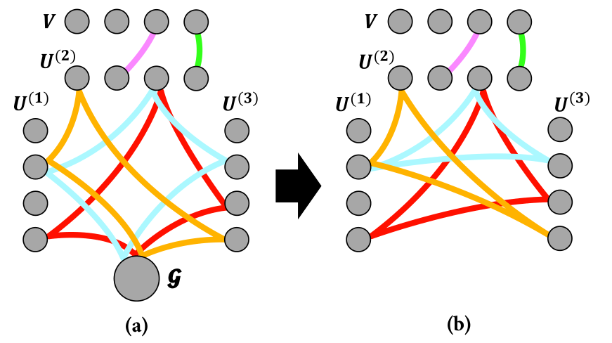
Definition 3.1.
Lock-free parallel update guarantees near linear convergence property of a sparse SGD problem in which conflicts between different updates rarely occur (Recht et al., 2011). However, in our formulation, every update of tensor entries includes the core tensor as shown in Figure 3a. We allocate the update of core tensor to one core to solve the problem. Then we obtain a new induced hypergraph in Figure 3b. The newly obtained hypergraph satisfies the sparsity condition for convergence. Lemma 3.2 proves the convergence property of parallel updates.
Lemma 3.2.
(Convergence) If we assume that the elements of the tensor and coupled matrix are sampled uniformly at random, lock-free parallel update of CMTF converges to a local optimum.
Proof.
For brevity, we assume that the dimension and rank of each mode are and , respectively. We use the notations used in Equation (2.6) of (Recht et al., 2011). For a given hypergraph , we define
First, consider the case when the tensor order is 2. has the same value, and has doubled value of the matrix factorization problem in (Recht et al., 2011): , . naturally satisfies . Next, when the tensor order is N, linearly scales up and , and stay same: , . Parallel update converges as proved in Proposition 4.1 of (Recht et al., 2011). ∎
3.4. CMTF-naive
We present a basic version of our method, CMTF-naive. CMTF-naive solves the sparse CMTF problem by parallel SGD techniques explained in Sections 3.2-3.3. Algorithm 1 shows the procedure of CMTF-naive. In the beginning, CMTF-naive initializes factor matrices and core tensor randomly (line 1 of Algorithm 1). The outer loop (lines 2-16) repeats until the factor variables converge. The inner loop (lines 3-14) is conducted by several cores in parallel except for line 7. In each inner loop, CMTF-naive selects an index which belongs to or in random order (line 3). If a tensor index is picked, then the algorithm calculates the partial gradients of corresponding factor rows using compute_gradient (Algorithm 2) in line 5, and updates factor row vectors (line 6). Core tensor is updated by only one core (line 7); the number of cores is multiplied to the gradient to compensate for the one-core update so that SGD uses the same learning rate for all the parameters. If a coupled matrix index is picked, then the gradient update is conducted on corresponding factor row vectors (lines 9-13). At the end of the outer loop, the learning rate is monotonically decreased (Bottou, 2012). (line 15). QR decomposition is applied on factors to satisfy orthogonality constraint of factor matrices (lines 17-20). QR decomposition of generates , an orthogonal matrix of the same size as , and a square matrix . Substituting by (line 19) and by (after -th execution of line 19) result in an equivalent factorization (Kolda, 2006). In the same manner, we substitute by (line 21) because .
3.5. CMTF-opt
Reusing the intermediate data. There are many redundant calculations in CMTF-naive. For example, is calculated for every execution of compute_gradient (Algorithm 2) in line 5 of Algorithm 1. In CMTF-opt, we save the time by storing the intermediate data of calculating and reusing them.
Definition 3.3.
(Intermediate Data) When updating the factor rows for a tensor entry , we define ()-th element of intermediate data :
There is no extra time required for calculating because is generated while calculating . Lemma 3.4 shows that is calculated by summing all entries of .
Lemma 3.4.
For a given tensor index , estimated tensor entry .
Proof.
The proof is straightforward by Equation (4). ∎
We use to calculate gradients efficiently.
Definition 3.5.
(Collapse)
The Collapse operation of the intermediate tensor on the -th mode outputs a row vector defined by
Collapse operation aggregates the elements of intermediate tensor with respect to a fixed mode. We re-express the calculation of gradients for tensor factors in Equations (8) in an efficient manner.
Lemma 3.6.
(Efficient Gradient Calculation) Followings are equivalent calculations of tensor factors gradients as Equations (8).
| (9) |
| (10) |
| (11) |
where and is element-wise division.
Proof.
In Lemma 3.4, Equation (9) is proved. To prove the equivalence of Equation (10) and the first equation of Equations (8), it suffices to show where and . We use Equation (3) for the proof.
Next, to show the equivalence of Equation (11) and the second equation of Equations (8), it suffices to show .
∎
CMTF-opt replaces compute_gradient (Algorithm 2) of CMTF-naive with compute_gradient_opt (Algorithm 3), a time-improved alternative using Lemma 3.6. We prove that the new calculation scheme is faster than the previous one.
Lemma 3.7.
compute_gradient_opt is faster than compute_gradient. The time complexity of compute_gradient is and the time complexity of compute_gradient_opt is where .
Proof.
We assume that for brevity. First, we calculate the time complexity of compute_gradient (Algorithm 2). Given a tensor index , computing (line 1 of Algorithm 2) takes . Computing () (line 3) takes . Thus, aggregate time for calculating the row gradient for all modes (lines 2-4) takes . Calculating (line 5) takes . In sum, compute_gradient takes time. Next, we calculate the time complexity of compute_gradient_opt (Algorithm 3). Computing an entry of intermediate data (line 3 of Algorithm 3) takes . Aggregate time for getting (lines 2-5) is because . Calculating row gradient for all modes (lines 6-8) takes because operation takes . Calculating gradient for core tensor (line 9) takes . In sum, compute_gradient_opt takes time. ∎
| Time complexity (per iter.) | Memory usage | |
|---|---|---|
| CMTF-naive | * | |
| CMTF-opt | * | |
| CMTF-Tucker-ALS | ||
| CMTF-OPT |
3.6. Analysis
We analyze the proposed method in terms of time complexity per iteration. For simplicity, we assume that , and . Table 3 summarizes the time complexity (per iteration) and memory usage of CMTF and other methods. Note that the memory usage refers to the auxiliary space for temporary variables used by a method.
Lemma 3.8.
The time complexity (per iteration) of CMTF-naive is and the time complexity (per iteration) of CMTF-opt is where denotes the number of parallel cores.
Proof.
First, we check the time complexity of CMTF-naive (Algorithm 1). When a tensor index is picked in the inner loop (line 4 of Algorithm 1), calculating gradients with respect to tensor factors (line 5) takes as shown in Lemma 3.7. Updating factor rows (line 6) takes , and updating core tensor (line 7) takes . If a coupled matrix index is picked (line 9), calculating (line 10) takes . Calculating and updating the factor rows corresponding to coupled matrix entry (lines 10-12) take . All calculations except updating core tensor (line 7) are conducted in parallel. Finally, for all and , CMTF-naive takes for one iteration. CMTF-opt uses compute_gradient_opt instead of compute_gradient in line 5 of Algorithm 1, whose time complexity is shown in Lemma 3.7. Overall running time per iteration for CMTF-opt is . ∎
4. Experiments
In this and the next sections, we experimentally evaluate CMTF. Especially, we answer the following questions.
Q1 : Performance (Section 4.2) How accurate and fast is CMTF compared to competitors?
Q2 : Scalability (Section 4.3) How do CMTF and other methods scale in terms of dimension, the number of observed entries, and the number of cores?
Q3 : Discovery (Section 5) What are the discoveries of applying CMTF on real-world data?
| Name | Data | Dimensionality | # entries | Density |
|---|---|---|---|---|
| MovieLens | User-Movie-Time | 71K-11K-157 | 10M | |
| Movie-Genre | 20 | 214K | 1 | |
| Netflix | User-Movie-Time | 480K-18K-74 | 100M | |
| Movie-Yearmonth | 110 | 2M | 1 | |
| Yelp | User-Business-Time | 1M-144K-149 | 4M | |
| User-User | 1M | 7M | ||
| Business-Category | 1K | 172M | 1 | |
| Business-City | 1K | 126M | 1 | |
| Synthetic | 3-mode tensor | 1K100M | 1K100M | |
| Matrix | 1K100M | 1K100M |
4.1. Experimental Settings
Data. Table 4 shows the data we used in our experiments. We use three real-world datasets (MovieLens11 1 http://grouplens.org/datasets/movielens/10m, Netflix22 2 http://www.netflixprize.com, and Yelp33 3 http://www.yelp.com/dataset_challenge) and generate synthetic data to evaluate CMTF. Each entry of the real-world datasets represents a rating, which consists of (user, ‘item’, time; rating) where ‘item’ indicates ‘movie’ for MovieLens and Netflix, and ‘business’ for Yelp. We use (movie, genre) and (movie, year) as coupled matrices for MovieLens and Netflix, respectively. We use (user, user) friendship matrix, (business, category) and (business, city) matrices for Yelp. We generate 3-mode synthetic random tensors with dimensionality and corresponding coupled matrices. We vary in the range of 1K100M and the number of tensor entries in the range of 1K100M. We set the number of entries as for synthetic coupled matrices.
Measure. We use test RMSE as the measure for tensor reconstruction error.
where is the index set of the test tensor, represents each test tensor entry, and is the corresponding reconstructed value.
Methods. We compare CMTF-naive and CMTF-opt with other single machine CMTF methods: CMTF-Tucker-ALS and CMTF-OPT (described in Section 2.3). To examine multi-core performance, we run two versions of CMTF-opt: CMTF-opt1 (1 core), and CMTF-opt20 (20 cores). We exclude distributed CMTF methods (Jeon et al., 2016a; Jeon et al., 2015; Beutel et al., 2014) because they are designed for Hadoop with multiple machines, and thus take too much time for single machine environment. For example, (Oh et al., 2017) reported that HaTen2 (Jeon et al., 2015) takes 10,700s to decompose 4-way tensor with and , which is almost 7,000 slower than a single machine implementation of CMTF-opt. For CMTF-Tucker-ALS, we use a MATLAB implementation based on Tucker-MET (Kolda and Sun, 2008). For CMTF-OPT, we use MATLAB implementation of CMTF Toolbox 1.144 4 http://www.models.life.ku.dk/joda/CMTF_Toolbox. We implement CMTF with C++, and OpenMP library for multi-core parallelization. We note for fair comparison that a fully optimized C++ implementation might be faster than MATLAB implementation for loop-oriented algorithms; on the other hand, MATLAB potentially beats C++ on matrix and array calculations due to its high-degree optimization and auto multi-core calculations. Regardless of the implementation environment, however, our main contributions still holds: CMTF scales to large data and a number of cores with high accuracy thanks to the careful use of intermediate data, while competitors fail with out-of-memory error due to their excessive memory usage.
We conduct all experiments on a machine equipped with Intel Xeon E5-2630 v4 2.2GHz CPU and 256GB RAM. All parameters are set to the best found values. We mark out-of-memory (O.O.M.) error when the memory usage exceeds the limit and out-of-time (O.O.T.) error when the iteration time exceeds seconds.
Parameters. We set pre-defined parameters: tensor rank , regularization factor , , the initial learning rate , and decay rate . We set to 0.1, , and for all datasets. For rank and initial learning rate, MovieLens: , Netflix: , and Yelp: .
4.2. Performance of
We measure the performance of CMTF to answer Q1. As seen in Figure 1 and 4, CMTF improves the test error of existing methods by 2.14.1 and decreases the running time for one iteration by 1143. The details of the experiments are as follows.
Accuracy. We divide each data tensor into 80%/20% for train/test sets. The lower error for a same elapsed time implies the better accuracy and faster convergence. Figure 1 shows the changes of test RMSE of each method on three datasets over elapsed time which are the answers for Q1. CMTF achieves the lowest error compared to others for the same elapsed time. For Netflix and Yelp, CMTF-Tucker-ALS shows O.O.M. error. On MovieLens, the best error of competitors is 2.904 of CMTF-OPT. In the same elapsed time, CMTF-opt20 achieves lower error, 0.8037. For Netflix, we improve the error of CMTF-OPT (3.764) by to achieve 0.9147. In Yelp, the best error of CMTF-OPT is 2.663. CMTF-opt20 shows the lowest error of 1.253 in a few tens of iterations, and after then, it falls into an over-fitting zone. CMTF-opt20 achieves less error than the best of CMTF-OPT.

Running time. We empirically show that CMTF achieves the best speed in terms of running time. Figure 4 shows the average running time of each method on the three data. CMTF-opt20 improves the running time of the best competitor by more than an order of magnitude for all datasets. In Yelp, CMTF-opt20 takes 25s for an iteration which is faster than 283s of CMTF-OPT. In MovieLens, CMTF-opt20 takes 18s, faster compared to 415s of CMTF-OPT. For Netflix, CMTF-opt20 achieves faster running time (140s) compared to that of CMTF-opt (6,100s). Note that CMTF-Tucker-ALS shows O.O.M. error for all data except for MovieLens. Though CMTF-naive and CMTF-opt1 show comparable running times to that of CMTF-OPT for an iteration, they converge faster and are more accurate as shown in Figure 1 since they capture inter-relations between factors with higher model capacities.
We compare our method with the multi-core version of SALS-single (Shin et al., 2017), a CP decomposition algorithm, to demonstrate the high performance of CMTF compared to up-to-date decomposition algorithms. We implement CP version of our method, CMTF-CP, by setting to be hyper-diagonal. Since CMTF is the extended problem of tensor decomposition, CMTF is used for tensor decomposition in a straightforward way by not coupling any matrices. CMTF-TUCKER denote the non-coupled version of CMTF-opt. MovieLens tensor is used for decomposition. Figure 6 shows that CMTF is better than SALS-single in terms of both error and time.
4.3. Scalability Analysis
We inspect scalability of our proposed method and others to answer Q2, in terms of two aspects: data scalability and parallel scalability. We use synthetic data of varying size for evaluation. As a result, we show the running time (for one iteration) of CMTF follows our theoretical analysis in Section 3.6.
Data Scalability. The time complexity of CMTF-Tucker-ALS and CMTF-OPT have and as their dominant terms, respectively. In contrast, CMTF exploits the sparsity of input data, and has the time complexity linear to the number of entries (, ) and independent to the dimensionality () as shown in Lemma 3.8. Figures 5a and 5b show that the running time (for one iteration) of CMTF follows our theoretical analysis in Section 3.6.
First, we fix to 1M and to 100K, and vary dimensionality from 1K to 100M. Figure 5a shows the running time (for one iteration) of all methods. Note that all our proposed methods achieve constant running time as dimensionality increases because they exploit the sparsity of data by updating factors related to only observed data entries. However, CMTF-Tucker-ALS shows O.O.M. when , and CMTF-OPT presents O.O.T. when . Next, we investigate the data scalability over the number of entries. We fix to 10K and raise from 10K to 100M. CMTF-Tucker-ALS shows O.O.M. when , and CMTF-OPT shows near-linear scalability. Focusing on the results of CMTF, all three versions of our approach show linear relation between running time and .
Parallel Scalability. We conduct experiments to examine parallel scalability of CMTF on shared memory systems. For measurement, we define Speed up as (Iteration time on 1 core)/(Iteration time). Figure 5c shows the linear Speed up of CMTF-naive and CMTF-opt. CMTF-opt earns higher Speed up than CMTF-naive because it reduces reading accesses for core tensor by utilizing intermediate data.
5. Discovery
| Cluster |
Location /
Category |
Top-10 Businesses |
|---|---|---|
| C1 |
Las Vegas, US/
Travel & Entertainment |
Nocturnal Tours, Eureka Casino, Happi Inn, Planet Hollywood Poker Room, Circus Midway Arcade, etc. |
| C2 |
Arizona, US/
Real estate & Home services |
ENMAR Hardwood Flooring, Sprinkler Dude LLC, Eklund Refrigeration, NR Quality Handyman, The Daniel Montez Real Estate Group, etc. |
| C11 |
Ontario, Canada/
Restaurants & Deserts |
Jyuban Ramen House, Tim Hortons, Captain John Donlands Fish and Chips, Cora’s Breakfast & Lunch, Pho Pad Thai, etc. |
| C17 |
Ohio, US/
Food & Drinks |
ALDI, Pulp Juice and Smoothie Bar, One Barrel Brewing, Wok N Roll Food Truck, Gas Pump Coffee Company, etc. |
In this section, we use CMTF for mining real-world data, Yelp, to answer the question Q3 in the beginning of Section 4. First, we demonstrate that CMTF has better discernment for business entities compared to the naive decomposition method by jointly capturing spatial and categorical prior knowledge. Second, we show how CMTF is possibly applied to the real recommender systems. It is an open challenge to jointly capture the spatio-temporal context along with user preference data (Gao et al., 2013). We exemplify a personal recommendation for a specific user. For discovery, we use the total Yelp data tensor along with coupled matrices as explained in Table 4. For better interpretability, we found non-negative factorization by applying projected gradient method (Lin, 2007). Orthogonality is not applied to keep non-negativity, and each column of factors is normalized.
Cluster Discovery. First, we compare discernment by CMTF and the Tucker decomposition. We use the business factor . Figure 7 shows gap statistic values of clustering business entities with k-means clustering algorithm. Higher gap statistic value means higher clustering ability (Tibshirani et al., 2001), thus CMTF outperforms the Tucker decomposition for entity clustering.
As the difference between CMTF and the Tucker decomposition is the existence of coupled matrices, the high performance of CMTF is attributed to the unified factorization using spatial and categorical data as prior knowledge. Table 5 shows the found clusters of business entities. Note that each cluster represents a certain combination of spatial and categorical characteristics of business entities.
User-specific recommendation. Commercial recommendation is one of the most important applications of factorization models (Koren et al., 2009; Karatzoglou et al., 2010). Here we illustrate how factor matrices are used for personalized recommendations with a real example. Figure 8 shows the process for recommendation. Below, we illustrate the process in detail.
- •
An example user Tyler has a factor vector , namely user profile, which has been calculated by previous review histories.
- •
We then calculate the personalized profile matrix . measures the amount of interaction of user profile with business and time factors.
- •
Norm values of rows in indicate the influence of latent business concepts on Tyler. Dominant and weak concepts are found based on the calculated norm values. In the example, B4 is the strong, and B7 is the weak latent concept.
- •
We inspect the corresponding columns of business factor matrix and find relevant business entities with high values for the found concepts (B4 and B7).
We found both strong and weak entities by the above process. The strong and weak entities provide recommendation information by themselves in the sense that the probability of the user to like strong and weak entities are high and low, respectively, and they also give extended user preference information. For example, strong entities for Tyler are related to ‘spa & health’ and located in neighborhood cities of Arizona, US. Weak entities are related to ‘grill & restaurants’ and located in Toronto, Canada. The captured user preference information makes commercial recommender systems more powerful with additional user-specific information such as address, current location, etc.

6. Conclusion
We propose CMTF, a fast, accurate, and scalable CMTF method. CMTF significantly decreases the running time by lock-free parallel SGD update and reusing intermediate data. CMTF boosts up prediction accuracy by exploiting the sparsity of data, and inter-relations between factors. CMTF shows 2.14.1 less error compared to the previous methods and improves the running time by 1143. CMTF shows linear scalability for the number of data entries and parallel cores. Moreover, we show the usefulness of CMTF for cluster analysis and recommendation by applying CMTF to a real-world data Yelp. Future works include extending the method to a distributed setting.
References
- Acar et al. (2011) Evrim Acar, Tamara G Kolda, and Daniel M Dunlavy. 2011. All-at-once optimization for coupled matrix and tensor factorizations. arXiv preprint arXiv:1105.3422 (2011).
- Acar et al. (2013) Evrim Acar, Morten Arendt Rasmussen, Francesco Savorani, Tormod Næs, and Rasmus Bro. 2013. Understanding data fusion within the framework of coupled matrix and tensor factorizations. Chemometrics and Intelligent Laboratory Systems 129 (2013), 53–63.
- Beutel et al. (2014) Alex Beutel, Partha Pratim Talukdar, Abhimanu Kumar, Christos Faloutsos, Evangelos E Papalexakis, and Eric P Xing. 2014. Flexifact: Scalable flexible factorization of coupled tensors on hadoop. In Proceedings of the 2014 SIAM International Conference on Data Mining. SIAM, 109–117.
- Bottou (2012) Léon Bottou. 2012. Stochastic gradient descent tricks. In Neural networks: Tricks of the trade. Springer, 421–436.
- Bradley et al. (2011) Joseph K Bradley, Aapo Kyrola, Danny Bickson, and Carlos Guestrin. 2011. Parallel coordinate descent for l1-regularized loss minimization. arXiv preprint arXiv:1105.5379 (2011).
- De Lathauwer et al. (2000) Lieven De Lathauwer, Bart De Moor, and Joos Vandewalle. 2000. On the best rank-1 and rank-(r 1, r 2,…, rn) approximation of higher-order tensors. SIAM journal on Matrix Analysis and Applications 21, 4 (2000), 1324–1342.
- Ding et al. (2008) Chris Ding, Tao Li, and Wei Peng. 2008. On the equivalence between non-negative matrix factorization and probabilistic latent semantic indexing. Computational Statistics & Data Analysis 52, 8 (2008), 3913–3927.
- Gao et al. (2013) Huiji Gao, Jiliang Tang, Xia Hu, and Huan Liu. 2013. Exploring temporal effects for location recommendation on location-based social networks. In Proceedings of the 7th ACM conference on Recommender systems. ACM, 93–100.
- Jeon et al. (2016a) ByungSoo Jeon, Inah Jeon, Lee Sael, and U Kang. 2016a. Scout: Scalable coupled matrix-tensor factorization-algorithm and discoveries. In Data Engineering (ICDE), 2016 IEEE 32nd International Conference on. IEEE, 811–822.
- Jeon et al. (2016b) Inah Jeon, Evangelos E. Papalexakis, Christos Faloutsos, Lee Sael, and U. Kang. 2016b. Mining billion-scale tensors: algorithms and discoveries. VLDB J. 25, 4 (2016), 519–544.
- Jeon et al. (2015) Inah Jeon, Evangelos E Papalexakis, U Kang, and Christos Faloutsos. 2015. Haten2: Billion-scale tensor decompositions. In Data Engineering (ICDE), 2015 IEEE 31st International Conference on. IEEE, 1047–1058.
- Karatzoglou et al. (2010) Alexandros Karatzoglou, Xavier Amatriain, Linas Baltrunas, and Nuria Oliver. 2010. Multiverse recommendation: n-dimensional tensor factorization for context-aware collaborative filtering. In Proceedings of the fourth ACM conference on Recommender systems. ACM, 79–86.
- Kiers et al. (1997) Henk AL Kiers, Jos MF Ten Berge, and Roberto Rocci. 1997. Uniqueness of three-mode factor models with sparse cores: The 3 3 3 case. Psychometrika 62, 3 (1997), 349–374.
- Kolda (2006) Tamara Gibson Kolda. 2006. Multilinear operators for higher-order decompositions. Technical Report. Sandia National Laboratories.
- Kolda and Bader (2009) Tamara G Kolda and Brett W Bader. 2009. Tensor decompositions and applications. SIAM review 51, 3 (2009), 455–500.
- Kolda and Sun (2008) Tamara G Kolda and Jimeng Sun. 2008. Scalable tensor decompositions for multi-aspect data mining. In Data Mining, 2008. ICDM’08. Eighth IEEE International Conference on. IEEE, 363–372.
- Koren et al. (2009) Yehuda Koren, Robert Bell, and Chris Volinsky. 2009. Matrix factorization techniques for recommender systems. Computer 42, 8 (2009).
- Lin (2007) Chih-Jen Lin. 2007. Projected gradient methods for nonnegative matrix factorization. Neural computation 19, 10 (2007), 2756–2779.
- Narita et al. (2012) Atsuhiro Narita, Kohei Hayashi, Ryota Tomioka, and Hisashi Kashima. 2012. Tensor factorization using auxiliary information. Data Mining and Knowledge Discovery 25, 2 (2012), 298–324.
- Oh et al. (2017) Jinoh Oh, Kijung Shin, Evangelos E Papalexakis, Christos Faloutsos, and Hwanjo Yu. 2017. S-HOT: Scalable High-Order Tucker Decomposition. In Proceedings of the Tenth ACM International Conference on Web Search and Data Mining. ACM, 761–770.
- Ozcaglar (2012) Cagri Ozcaglar. 2012. Algorithmic data fusion methods for tuberculosis. Ph.D. Dissertation. Rensselaer Polytechnic Institute.
- Papalexakis et al. (2014) Evangelos E Papalexakis, Christos Faloutsos, Tom M Mitchell, Partha Pratim Talukdar, Nicholas D Sidiropoulos, and Brian Murphy. 2014. Turbo-smt: Accelerating coupled sparse matrix-tensor factorizations by 200x. In Proceedings of the 2014 SIAM International Conference on Data Mining. SIAM, 118–126.
- Peng and Li (2011) Wei Peng and Tao Li. 2011. On the equivalence between nonnegative tensor factorization and tensorial probabilistic latent semantic analysis. Applied Intelligence 35, 2 (2011), 285–295.
- Recht et al. (2011) Benjamin Recht, Christopher Re, Stephen Wright, and Feng Niu. 2011. Hogwild: A lock-free approach to parallelizing stochastic gradient descent. In Advances in neural information processing systems. 693–701.
- Rendle and Schmidt-Thieme (2010) Steffen Rendle and Lars Schmidt-Thieme. 2010. Pairwise interaction tensor factorization for personalized tag recommendation. In Proceedings of the third ACM international conference on Web search and data mining. ACM, 81–90.
- Sael et al. (2015) Lee Sael, Inah Jeon, and U Kang. 2015. Scalable Tensor Mining. Big Data Research 2, 2 (2015), 82 – 86. DOI:http://dx.doi.org/10.1016/j.bdr.2015.01.004 Visions on Big Data.
- Shin et al. (2017) Kijung Shin, Lee Sael, and U. Kang. 2017. Fully Scalable Methods for Distributed Tensor Factorization. IEEE Trans. Knowl. Data Eng. 29, 1 (2017), 100–113.
- Tibshirani et al. (2001) Robert Tibshirani, Guenther Walther, and Trevor Hastie. 2001. Estimating the number of clusters in a data set via the gap statistic. Journal of the Royal Statistical Society: Series B (Statistical Methodology) 63, 2 (2001), 411–423.
- Xu et al. (2003) Wei Xu, Xin Liu, and Yihong Gong. 2003. Document clustering based on non-negative matrix factorization. In Proceedings of the 26th annual international ACM SIGIR conference on Research and development in informaion retrieval. ACM, 267–273.