跳到论文正文
W Papers独立论文阅读器 arXiv:1708.08624 论文正文 计算阅读时间 · 0%
引用这篇论文根据当前论文元数据生成,正式投稿前建议核对。


License: arXiv.org perpetual non-exclusive license
arXiv:1708.08624v4 [hep-ph] 21 Nov 2017

Oct., 2017

Confronting Dirac Fermionic Dark Matter with Recent Data

Chun-Khiang Chua, Gwo-Guang Wong

Department of Physics and Chung Yuan Center for High Energy Physics,

Chung Yuan Christian University,

Taoyuan, Taiwan 32023, Republic of China

Abstract

We study Dirac fermionic dark matter (DM, χ0\chi^{0}) and confront it with recent data. To evade the stringent direct search limits from PandaX-II, XENON1T and LUX experiments, the quantum numbers of the Dirac DM are taken to be I3=Y=0I_{3}=Y=0 to remove the tree-level ZZ-exchange diagram. Loop amplitudes can contribute to the elastic scattering cross section. We find that there are cancellations in the one-loop diagrams, which largely reduce the cross section and make the Dirac DM viable in the direct search. For a generic isospin II, we survey the Dirac DM mass constrained by the latest results of PandaX-II, XENON1T and LUX experiments, the observed DM relic density, and the H.E.S.S. and the Fermi-LAT astrophysical observations. Sommerfeld enhancement effects on DM annihilation processes are investigated. We find that the cross section of χ0​χ¯0\chi^{0}\bar{\chi}^{0} annihilating to the standard model (SM) gauge bosons are in general significantly enhanced, and the Fermi-LAT, the H.E.S.S. upper limits on ⟨σ​v⟩​(W+​W−,γ​γ)\langle\sigma v\rangle({W^{+}W^{-},\gamma\gamma}) and the observed relic density become serious constraints on the Dirac DM mass. The I<4I<4 cases are ruled out and for I≥4I\geq 4, the lower bound on Dirac DM mass are forced to be ≳\gtrsim 60 TeV. The elastic scattering cross section for mχm_{\chi} of few tens TeV with a generic II is found to be σS​I≃I2​(I+1)2×7×10−49\sigma^{SI}\simeq I^{2}(I+1)^{2}\times 7\times 10^{-49} cm2. The predicted ⟨σ(χ0χ¯0→Z0Z0,Z0γ,γγ)v⟩\langle\sigma(\chi^{0}\bar{\chi}^{0}\to Z^{0}Z^{0},Z^{0}\gamma,\gamma\gamma)v\rangle and σS​I\sigma^{SI} are sizable and they will be useful to search for DM in astrophysical observation and in direct search in near future.

I Introduction

The existence of dark matter (DM) in different astrophysical scales of the Universe [1, 2, 3, 4, 5, 6, 7] provides strong evidence for physics beyond the Standard Model (SM). Weakly interacting massive particles (WIMPs) are promising DM candidates. The WIMPs are assumed to be created thermally during the big bang, and froze out of thermal equilibrium escaping the Boltzmann suppression in the early Universe. The DM relic density is approximately related to the velocity averaged DM annihilation cross section by a simple relation [8],

Ωχ​h2≈0.1​pb×c<σ​v>.\displaystyle\Omega_{\chi}h^{2}\approx{\frac{0.1{\rm pb}\times c}{<\sigma v>}}. (1)

Comparing to the measured value of CDM relic density is [9]

Ωobs​h2=0.1186±0.0020,\displaystyle\Omega_{\rm obs}h^{2}=0.1186\pm 0.0020, (2)

it suggests the case of DM with mass in the range of 100 GeV to few TeV and governed by an electroweak size interaction. That is well known as the €WIMP miracle [10]€.

There are three complementary searching strategies to detect the DM particles in experiments (see [10, 11] for brief reviews). They are the direct detection of DM-nucleus scattering in underground laboratories, the indirect detection of DM annihilation processes in astrophysical observation and the DM direct production at colliders [10, 11, 12, 13, 14, 15, 16, 17, 18, 19, 20]. So far these searches only provide upper limits. Recently upper limits on spin-independent (SI), spin-dependent (SD) DM-nucleus scattering cross sections are reported by PandaX-II [21], XENON1T [22], LUX [23, 24] experiment groups, while that on velocity averaged DM annihilation cross sections are from H.E.S.S [25, 26] and Fermi-LAT [27] groups. In spite of the fact that DM contains about 85%85\% for the total mass in the universe [28, 29], we still do not know much about its nature. In the literature, the possibilities of DM particle as a scalar [30, 31, 32, 33, 34, 35, 36], fermion [8, 37, 38, 39, 40, 41, 42, 46, 43, 44, 45, 47, 49, 48, 50] or a vector boson [54, 51, 52, 53, 55, 56, 57, 58, 59, 60, 50] are considered.

In this paper, we study the case of a Dirac fermionic DM. We investigate a renormalizable DM model by introducing a pure weak eigenstate Dirac fermion as a DM candidate. The DM only interacts through gravity and weak interactions [40, 41, 44]. We will confront the model to the recent experimental data of relic density, direct and indirect detection experiments.

This paper is organized as follows. In Sec. II we introduce the model. In Sec. III we calculate the cross sections of DM-nucleus elastic scattering and compare them with the results of recent LUX, XENON1T and PandaX-II experiments in the direct search. In Sec. IV we calculate the velocity averaged cross section of DM annihilating to the SM particles and the DM relic density incorporating the Sommerfeld enhancement effect. We compare our results with the Fermi-LAT and the H.E.S.S data and the observed relic density, respectively. Conclusions are given in Sec. V. We collect the loop integral functions in Appendix A, followed by a comprehensive derivation of Sommerfeld factors in Appendix B.

II A Dirac fermionic dark matter model

We introduce a Dirac fermionic dark matter model by adding on SM a Dirac fermionic multiplet χ\chi with arbitrary II and YY, and the Lagrangian can be written as [40, 41, 44]

ℒ\displaystyle{\cal L} =\displaystyle= ℒS​M+χ¯​(i​γμ​Dμ−mχ)​χ\displaystyle{\cal L}_{SM}+{\bar{\chi}}(i\gamma^{\mu}D_{\mu}-m_{\chi})\chi (3)
=\displaystyle= ℒS​M+χ¯jγμ(i∂μ−gWμaTj​ka+g′BμYjδj​k)χk−mχχ¯iχi,\displaystyle{\cal L}_{SM}+{\bar{\chi}^{j}}\gamma^{\mu}(i\partial_{\mu}-gW^{a}_{\mu}T^{a}_{jk}+g^{\prime}B_{\mu}Y_{j}\delta_{jk})\chi^{k}-m_{\chi}\bar{\chi}^{i}\chi^{i},

where WμaW^{a}_{\mu} and BμB_{\mu} are the familiar electroweak SU​(2)L\rm{SU(2)_{L}} and U⁡(1)\rm{U(1)} gauge fields, respectively. In this model, the SM is minimally extended so that the DM can only interact with the SM gauge bosons. Besides, there is only one free parameter, the DM mass mχm_{\chi} that makes the model predictive. As in most DM models, an addition discrete symmetry is needed to assure the stability of DM. For example, we may assign the Dirac DM with Z2Z_{2}-odd quantum number and the SM particles with a Z2Z_{2}-even quantum number to maintain the stability of DM.

The Lagrangian for the WIMPs interacting with the SM gauge bosons can be extracted from Eq.(3), giving

ℒ′\displaystyle{\cal L^{\prime}} =\displaystyle= −g2χ¯jγμ(Wμ+Tj​k++Wμ−Tj​k−)χk−χ¯jγμ[(gcosθWTj​k3−g′sinθWYjδj​k)Zμ+eAμQ)]χk.\displaystyle-\frac{g}{\sqrt{2}}{\bar{\chi}^{j}}\gamma^{\mu}(W^{+}_{\mu}T^{+}_{jk}+W^{-}_{\mu}T^{-}_{jk})\chi^{k}-{\bar{\chi}^{j}}\gamma^{\mu}[(g\cos\theta_{W}T^{3}_{jk}-g^{\prime}\sin\theta_{W}Y_{j}\delta_{jk})Z_{\mu}+eA_{\mu}Q)]\chi^{k}. (4)

Here we have used the weak mixing angle θW\theta_{W} and the relation e=gsinθW=g′cosθWe=g\sin\theta_{W}=g^{\prime}\cos\theta_{W} with electric charge Q=T3+YQ=T^{3}+Y. As the DM is electrically neutral, the Lagrangian for DM interacting with ZZ-boson can be further extracted as

ℒ′χ0=−gcos⁡θW​T3​χ¯0​γμ​χ0​Zμ.\displaystyle{\cal L^{\prime}}_{\chi^{0}}=-\frac{g}{\cos\theta_{W}}T^{3}{\bar{\chi}^{0}}\gamma^{\mu}\chi^{0}Z_{\mu}. (5)

The tree-level vector interaction of DM with ZZ-boson leads to the SI elastic cross section with a nucleus NN:

σASI​(χ​N→χ​N)=μN24​π​(gcos⁡θW​MZ)4​I32​[−14​(A−Z)+(14−sin⁡θw2)​Z]2,\displaystyle\sigma^{\rm SI}_{A}(\chi N\rightarrow\chi N)=\frac{\mu^{2}_{N}}{4\pi}\bigg(\frac{g}{\cos\theta_{W}M_{Z}}\bigg)^{4}I_{3}^{2}\bigg[-\frac{1}{4}(A-Z)+(\frac{1}{4}-\sin\theta_{w}^{2})Z\bigg]^{2}, (6)

where ZZ and AA are the numbers of protons and nucleons in the target nucleus respectively, I3I_{3} is the weak isospin quantum number and μN\mu_{N} is the of DM-nucleus reduced mass. It corresponds to the normalized cross section with a nucleon:

σp,nS​I≃I32×10−39​cm2,\displaystyle\sigma^{SI}_{p,n}\simeq I^{2}_{3}\times 10^{-39}{\rm cm^{2}}, (7)

for mχm_{\chi} ranges from a few GeV to a few 100 TeV.

The above cross section has already been ruled out in the direct search of SI-experiments of DM-nucleus scattering for many years, unless the quantum numbers of the Dirac DM are either (i) I≠0,I3=Y=0I\neq 0,I_{3}=Y=0 or (ii) I=Y=0I=Y=0 [44]. In this model, we shall consider the first case, i.e. I≠0I\neq 0, but I3=Y=0I_{3}=Y=0. Nevertheless, we still need to check the contribution to the SI elastic cross section from loop diagram.

As we know that the DM is highly nonrelativistic in the DM-nucleus elastic scattering. In literature, the loop contributions to DM-nucleus elastic cross section are explored in the Majorana fermionic DM case [61, 62, 63]. In this paper we will study the loop contribution to the elastic DM-nucleus scattering in the Dirac fermionic DM case.

III Dirac fermionic dark matter in the direct search

III.1 Effective Lagrangian

In this paper, we only consider the case: I≠0,I3=Y=0I\neq 0,I_{3}=Y=0. Hence the elastic cross section of Dirac DM-nucleus scattering is vanishing at tree level. Note that the Majorana fermionic DM case were studied in [41, 61]. The effective Lagrangian of Dirac DM with quarks and gluon can be written as [8, 62]

ℒeff\displaystyle{\cal L}^{\rm eff} =\displaystyle= ∑q=u,d,sℒqeff+ℒgeff,\displaystyle\sum_{q=u,d,s}{\cal L}^{\rm eff}_{q}+{\cal L}^{\rm eff}_{g}, (8)
ℒqeff\displaystyle{\cal L}^{\rm eff}_{q} =\displaystyle= aq​[χ¯0​χ0]​[q¯​q]+bq​[χ¯0​γμ​χ0]​[q¯​γμ​q]+dq​[χ¯0​γμ​γ5​χ0]​[q¯​γμ​γ5​q]\displaystyle a_{q}[{\bar{\chi}^{0}}\chi^{0}][{\bar{q}}q]+b_{q}[{\bar{\chi}^{0}}\gamma^{\mu}\chi^{0}][{\bar{q}}\gamma_{\mu}q]+d_{q}[{\bar{\chi}^{0}}\gamma^{\mu}\gamma^{5}\chi^{0}][{\bar{q}}\gamma_{\mu}\gamma^{5}q] (9)
+\displaystyle+ gq(1)mχχ¯0i∂μγνχ0𝒪μ​νq+gq(2)mχχ¯0(i∂μ)(i∂ν)χ0𝒪μ​νq,\displaystyle\frac{g_{q}^{(1)}}{m_{\chi}}\bar{\chi}^{0}i\partial^{\mu}\gamma^{\nu}\chi^{0}{\cal O}_{\mu\nu}^{q}+\frac{g_{q}^{(2)}}{m_{\chi}}\bar{\chi}^{0}(i\partial^{\mu})(i\partial^{\nu})\chi^{0}{\cal O}_{\mu\nu}^{q},
ℒgeff\displaystyle{\cal L}^{\rm eff}_{g} =\displaystyle= fG​χ¯0​χ0​Gμ​νa​Ga​μ​ν.\displaystyle f_{G}{\bar{\chi}^{0}}\chi^{0}G_{\mu\nu}^{a}G^{a\mu\nu}. (10)

where the quark twist-2 operator, 𝒪μ​νq{\cal O}_{\mu\nu}^{q}, is defined as

𝒪μ​νq≡12​q¯​i​(Dμ​γν+Dν​γμ−12​gμ​ν​​D)​q.\displaystyle{\cal O}_{\mu\nu}^{q}\equiv\frac{1}{2}\bar{q}i\bigg(D_{\mu}\gamma_{\nu}+D_{\nu}\gamma_{\mu}-\frac{1}{2}g_{\mu\nu}\!\not{\!\!D}\bigg)q. (11)
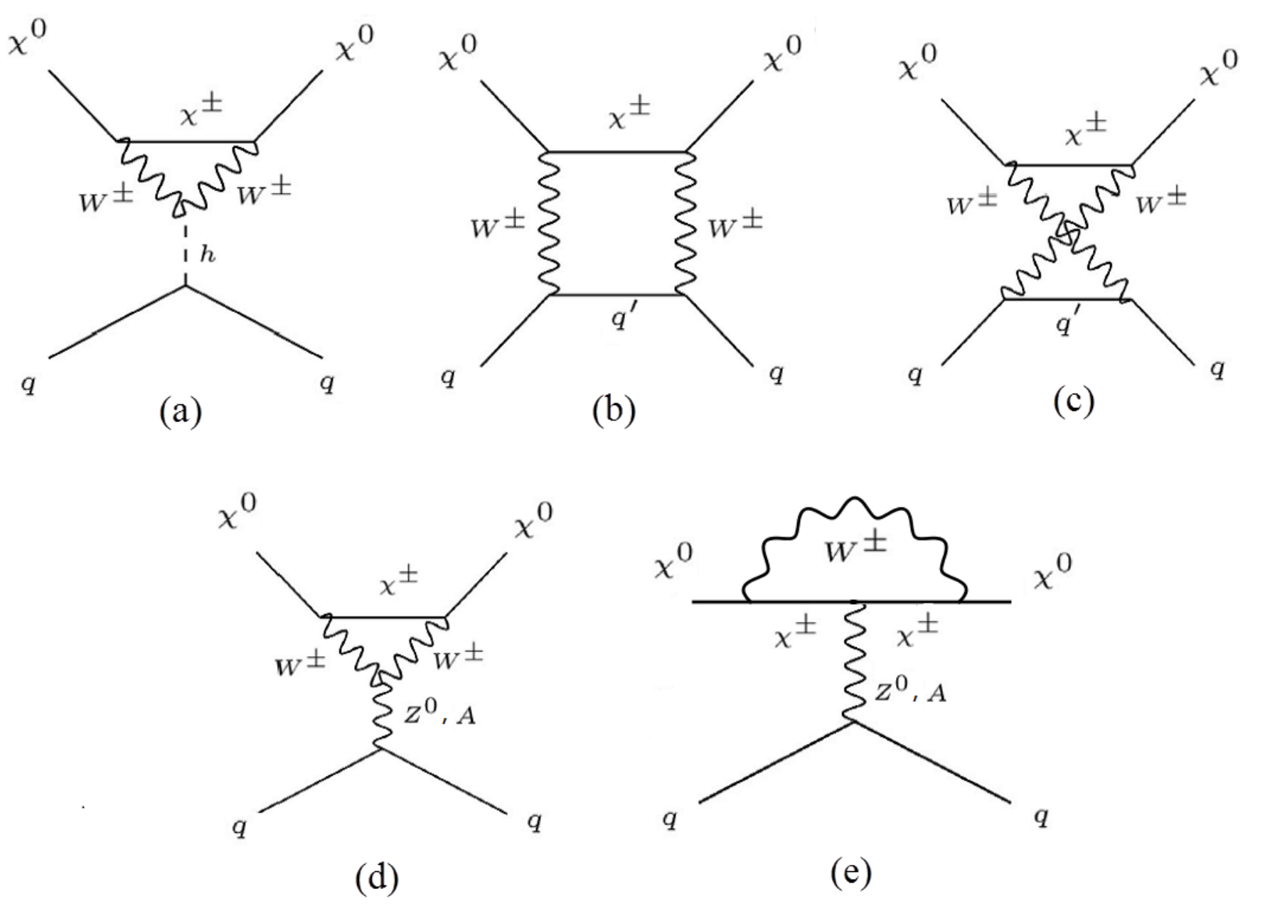
Refer to caption
Figure 1: One-loop diagrams for the effective interaction of Dirac DM with quarks

Fig. 1 shows the one-loop Feynman diagrams which induce the effective interactions of DM χ0\chi^{0} with quarks. Note that in the Dirac fermionic DM case, χ0\chi^{0} and χ¯0\bar{\chi}^{0} are different particles. There is an additional set of diagrams with χ0\chi^{0} in Fig. 1 replaced by χ¯0\bar{\chi}^{0}. These diagrams are related. In fact, one can show that the former amplitude Mχ0M_{\chi^{0}} is equal to latter one Mχ¯0M_{\bar{\chi}^{0}}. Now we let nχ0n_{\chi^{0}} and nχ¯0n_{\bar{\chi}^{0}} be the number density of the particle χ0\chi^{0} and the antipaticle χ¯0\bar{\chi}^{0}, respectively. They add up to the total number density of DM, nD​M=nχ0+nχ¯0n_{DM}=n_{\chi^{0}}+n_{\bar{\chi}^{0}}. Using Mχ0=Mχ¯0M_{\chi^{0}}=M_{\bar{\chi}^{0}}, we have nχ0​|Mχ0|2+nχ¯0​|Mχ¯0|2=(nχ0+nχ¯0)​|Mχ0|2=nD​M​|Mχ0|2n_{\chi}^{0}|M_{\chi^{0}}|^{2}+n_{\bar{\chi}^{0}}|M_{\bar{\chi}^{0}}|^{2}=(n_{\chi}^{0}+n_{\bar{\chi}^{0}})|M_{\chi^{0}}|^{2}=n_{DM}|M_{\chi^{0}}|^{2}. Hence we only need to calculate Mχ0M_{\chi^{0}}.

Note that the amplitudes correspond to the Feynman diagrams in Figs. 1 (d) and (e) turns out to be vanishing individually. Both diagrams have two sub-diagrams. The relative sign differences between the trilinear couplings of the vector bosons W+​W+​V0W^{+}W^{+}V^{0} and W−​W−​V0W^{-}W^{-}V^{0} (V0=ZV^{0}=Z or AA) are responsible for the cancelation of diagrams in Fig. 1 (d), while relative sign differences between the couplings χ−​χ−​V0\chi^{-}\chi^{-}V^{0} and χ+​χ+​V0\chi^{+}\chi^{+}V^{0} are responsible for vanishing of the sum of diagrams in Fig. 1 (e). 11 1 For example, the photon exchange diagram in Fig. 1 (d) contains two sub-diagrams: with χ+\chi^{+}, W−W^{-} or χ−\chi^{-}, W+W^{+} running in the loop. The corresponding matrix elements are M±\displaystyle M_{\pm} =\displaystyle= ∫d4​k(2​π)4[μ¯(p3)(−i2gT0±∓γμ′)(i​p1+​k−mχ)(−i2gT±0±γν′)u(p1)](−i​gμ​μ′(k+p1−p3)2−MW2)×\displaystyle\int\frac{d^{4}k}{(2\pi)^{4}}[{\bar{\mu}}(p_{3})(\frac{-i}{\sqrt{2}}gT^{\mp}_{0\pm}\gamma^{\mu^{\prime}})(\frac{i}{\!\not{\!p}_{1}+\!\not{\!k}-m_{\chi}})(\frac{-i}{\sqrt{2}}gT^{\pm}_{\pm 0}\gamma^{\nu^{\prime}})u(p_{1})](\frac{-ig_{\mu\mu^{\prime}}}{(k+p_{1}-p_{3})^{2}-M_{W}^{2}})\times (12) {∓isinθW[(p1−p3)λgμ​ν+(k−p3+p1)μgν​λ+(2p3−2p1−k)νgλμ]}(−i​gν​ν′k2−MW2)×\displaystyle\{\mp i\sin\theta_{W}[(p_{1}-p_{3})_{\lambda}g_{\mu\nu}+(k-p_{3}+p_{1})_{\mu}g_{\nu\lambda}+(2p_{3}-2p_{1}-k)_{\nu}g_{\lambda\mu]}\}(\frac{-ig_{\nu\nu^{\prime}}}{k^{2}-M_{W}^{2}})\times −i​gλ​κ(p3−p1)2​[u¯q​(p4)​(−i​Qq​e​γκ)​uq​(p2)],\displaystyle\frac{-ig_{\lambda\kappa}}{(p_{3}-p_{1})^{2}}[{\bar{u}}_{q}(p_{4})(-iQ_{q}e\gamma^{\kappa})u_{q}(p_{2})], where p1​(3)p_{1(3)} and p2​(4)p_{2(4)} are the momenta of incident (outgoing) χ\chi and qq, respectively, and T0+−=T+0+=T0−+=T−0−=I⁡(I+1)T^{-}_{0+}=T^{+}_{+0}=T^{+}_{0-}=T^{-}_{-0}=\sqrt{I(I+1)}. Consequently, we have M++M−=0M_{+}+M_{-}=0 from the relative sign difference between the trilinear couplings of the vector bosons W+​W+​AW^{+}W^{+}A and W−​W−​AW^{-}W^{-}A. Hence, only the Feynman diagrams in Figs. 1(a)-(c) contribute to the effective interactions.

We calculate the effective couplings aqa_{q}, bqb_{q} and dqd_{q} from Fig. 1 and use gq(1)g_{q}^{(1)}, gq(2)g_{q}^{(2)} obtained in Ref. [62]. In the nonrelativistic limit with mχ≫mt,mWm_{\chi}\gg m_{t},m_{W}, and ignoring the mass splitting among the neutral DM (χ0\chi^{0}) and the single charged WIMP partners (χ±\chi^{\pm}), we have 22 2 Our aqa_{q} and dqd_{q} agree with those in [62] up to an additional factor 2 for mχ≫mt,mWm_{\chi}\gg m_{t},m_{W}. Note that bq=0b_{q}=0 for Majorana DM in Ref. [62]. The additional factor is from the differences of the Lagrangians and amplitudes in the Dirac and Majorana cases. We apply the factor 2 to gq(1)g_{q}^{(1)} and gq(2)g_{q}^{(2)} when adapting the results from Ref. [62].

aq\displaystyle a_{q} =\displaystyle= I⁡(I+1)​g416​π2​[mqMW​mh2​FhS​(q,x,y)+mqMW3​FWS​(q,x,y)],\displaystyle I(I+1)\frac{g^{4}}{16\pi^{2}}\bigg[\frac{m_{q}}{M_{W}m^{2}_{h}}F^{S}_{h}(q,x,y)+\frac{m_{q}}{M^{3}_{W}}F^{S}_{W}(q,x,y)\bigg],
bq\displaystyle b_{q} =\displaystyle= I⁡(I+1)​g416​π2​[mqMW3​FW1V​(q,x,y)+1MW2​FW2V​(q,x,y)],\displaystyle I(I+1)\frac{g^{4}}{16\pi^{2}}\bigg[\frac{m_{q}}{M_{W}^{3}}F^{V}_{W_{1}}(q,x,y)+\frac{1}{M^{2}_{W}}F^{V}_{W_{2}}(q,x,y)\bigg],
dq\displaystyle d_{q} =\displaystyle= I⁡(I+1)​g416​π2​[1MW2​FW1A​(q,x,y)+1mχ2​FW2A​(q,x,y)],\displaystyle I(I+1)\frac{g^{4}}{16\pi^{2}}\bigg[\frac{1}{M_{W}^{2}}F^{A}_{W_{1}}(q,x,y)+\frac{1}{m^{2}_{\chi}}F^{A}_{W_{2}}(q,x,y)\bigg],
gq(1)\displaystyle g_{q}^{(1)} =\displaystyle= I⁡(I+1)​g416​π2​1MW3​gT​1​(x),\displaystyle I(I+1)\frac{g^{4}}{16\pi^{2}}\frac{1}{M_{W}^{3}}g_{T1}(x),
gq(2)\displaystyle g_{q}^{(2)} =\displaystyle= I⁡(I+1)​g416​π2​1MW3​gT​2​(x),\displaystyle I(I+1)\frac{g^{4}}{16\pi^{2}}\frac{1}{M_{W}^{3}}g_{T2}(x), (13)

where we define x≡MW2/mχ2x\equiv{M_{W}^{2}}/{m_{\chi}^{2}}, y≡mt2/mχ2y\equiv{m_{t}^{2}}/{m_{\chi}^{2}} with mqm_{q}, mtm_{t} and mWm_{W} the quark qq, tt and the WW-boson masses, respectively. Note that aqa_{q}, bqb_{q} and dqd_{q} contribute to the so-called SS, VV and AA interactions, respectively, while gq(1)g_{q}^{(1)} and gq(2)g_{q}^{(2)} also contribute to the SS interaction. All loop integral functions FhS​(q,x,y)F^{S}_{h}(q,x,y), FW1,2V,A​(q,x,y)F^{V,A}_{W_{1,2}}(q,x,y), gT​1​(x)g_{T1}(x) and gT​2​(x)g_{T2}(x) are collected in Appendix A.

The two-loop diagrams shown in Fig. 2 produce the effective scalar coupling of Dirac DM with gluon in a nucleon, fGf_{G} defined in Eq. (10). These diagrams contribute to the effective scalar coupling, fGf_{G} giving

fG=fG(a)+fG(b)+fG(c),\displaystyle f_{G}=f_{G}^{(a)}+f_{G}^{(b)}+f_{G}^{(c)}, (14)

where the superscripts correspond to the labels of the diagrams in Fig. 2. We use the results obtained in Ref. [62] for these fG(i)f_{G}^{(i)}.

Refer to caption
Figure 2: Two-loop diagrams contributing to the effective scalar coupling of Dirac DM with gluons.

The heavy quark contribution to the mass of the nucleon through the triangle diagram [73] shown in Fig. 2(a) gives the effective scalar coupling:

fG(a)=−αs12​π​g416​π2​I​(I+1)​cQ​14​mW​gH​(x)≃−αs12​π​aQmQ,\displaystyle f_{G}^{(a)}=-\frac{\alpha_{s}}{12\pi}\frac{g^{4}}{16\pi^{2}}I(I+1)c_{Q}\frac{1}{4m_{W}}g_{H}(x)\simeq-\frac{\alpha_{s}}{12\pi}\frac{a_{Q}}{m_{Q}}, (15)

where the loop integral function gH​(x)g_{H}(x) with x≡MW2/mχ2x\equiv{M_{W}^{2}}/{m_{\chi}^{2}} is basically from [62] and is collected in Appendix A, 33 3 Similarly, fG(i)​(i=a,b,c)f_{G}^{(i)}\ (i=a,b,c) used here have an additional factor of two compared to those in Ref. [62]. See footnote 2. cQ=1+11​αs​(mQ)/4​πc_{Q}=1+11\alpha_{s}(m_{Q})/4\pi with Q=c,b,tQ=c,b,t and aQa_{Q} is defined in Eq. (13). Note that in the above equation we have taken cQ=1c_{Q}=1 for Q=c,b,tQ=c,b,t for simplicity, while in Ref. [62], cc=1.32,cb=1.19c_{c}=1.32,c_{b}=1.19 and ct=1c_{t}=1 for αs​(mz)=0.118\alpha_{s}(m_{z})=0.118 are used. From Figs. 2(b) and (c), we have [62]

fG(b)+fG(c)=αs4​π​g416​π2​I​(I+1)​1MW3​gW​(x,y),\displaystyle f_{G}^{(b)}+f_{G}^{(c)}=\frac{\alpha_{s}}{4\pi}\frac{g^{4}}{16\pi^{2}}I(I+1)\frac{1}{M_{W}^{3}}g_{W}(x,y), (16)

the loop integral function gW​(x,y)g_{W}(x,y) with x≡MW2/mχ2x\equiv{M_{W}^{2}}/{m_{\chi}^{2}}, y≡mt2/mχ2y\equiv{m_{t}^{2}}/{m_{\chi}^{2}} is collected in Appendix A. Note that the contribution of the twist-2 operators of gluon which are suppressed by the strong coupling constant αs\alpha_{s} have been ignored (see Ref.[74]).

In Appendix A, the loop integral functions Fh,W1,2S,V,A​(q,x,y)F^{S,V,A}_{h,W_{1,2}}(q,x,y) can be classified into three classes as whether the external line in Fig. 1 involves light, bb or tt quarks. For the light quark case, we only keep the effective coupling up to the leading order in mqm_{q}. For the bb-quark case, the top quark is in the loop of the box diagrams and the loop integral functions can be analytically solved under the assumption: mχ≫mtm_{\chi}\gg m_{t}. For the tt-quark case, the bottom quark is in the loop of the box diagrams and the loop integral functions can only be numerically solved (with the assumption: mχ≫mtm_{\chi}\gg m_{t}). Note that there is a cancellation in the VV interaction so that the large component (∼1/MW2)(\sim 1/M^{2}_{W}) of the effective coupling bqb_{q} is vanishing for all quark flavors; in other words, FW​2V​(q,x,y)=0F^{V}_{W2}(q,x,y)=0. We will see later that it makes the Dirac DM model viable in the direct search. Note that a similar cancellation in the Majorana case was reported in Ref. [62].

III.2 Spin-independent and Spin-dependent Cross Sections

To compare with the results of recent PandaX-II [21], XENON1T [22] and LUX [23, 24] experiments, we calculate the normalized SI and SD cross sections of Dirac DM elastic scattering off Xe129,131{}^{129,131}{\rm Xe} nuclei. We shall obtain the averaged unpolarized amplitude squared ∑¯​|Mf​i|2\overline{\sum}|M_{fi}|^{2} at q2=0q^{2}=0 first. Note that there is no interference between various interaction terms in i​Mf​iiM_{fi}. From the effective Lagrangian of DM-nucleus elastic scattering, the unpolarized matrix element square can be written as [43]

∑¯​|Mf​i|2​(q2=0)\displaystyle\overline{\sum}|M_{fi}|^{2}(q^{2}=0) =\displaystyle= ∑¯​|Mf​iS​I|2​(q2=0)+∑¯​|Mf​iS​D|2​(q2=0)\displaystyle\overline{\sum}|M^{SI}_{fi}|^{2}(q^{2}=0)+\overline{\sum}|M^{SD}_{fi}|^{2}(q^{2}=0) (17)
=\displaystyle= 16​m𝒩2​mχ2​[(fs​𝒩2+QV​𝒩2)+4​QA​𝒩2​J𝒩​(J𝒩+1)].\displaystyle 16m_{\cal N}^{2}m^{2}_{\chi}\bigg[\bigg(f^{2}_{s\cal N}+Q_{V\cal N}^{2}\bigg)+4Q_{A\cal N}^{2}J_{\cal N}(J_{\cal N}+1)\bigg].

The first two terms are from the effective SS and VV interactions, respectively, contributing to |MS​I|2|M^{SI}|^{2}, while the last term from the AA interaction contributing to |MS​D|2|M^{SD}|^{2}.

For the VV interaction, we have

QV​𝒩\displaystyle Q_{V\cal N} =\displaystyle= Z⁡(2​bu+bd)+(A−Z)​(2​bd+bu).\displaystyle Z(2b_{u}+b_{d})+(A-Z)(2b_{d}+b_{u}). (18)

For the AA interaction, we have

QA​𝒩\displaystyle Q_{A\cal N} =\displaystyle= ∑q=u,d,sdq​(Δqp​λp+Δqn​λn),λp,n=⟨Sp,n⟩effJ𝒩,\displaystyle\sum_{q=u,d,s}d_{q}(\Delta_{q}^{p}\lambda_{p}+\Delta_{q}^{n}\lambda_{n}),\hskip 9.24994pt\lambda_{p,n}=\frac{\langle S_{p,n}\rangle_{\rm eff}}{J_{\cal N}}, (19)

where Δqp⁡(n)\Delta^{p(n)}_{q} is the quark spin component in proton (neutron), ⟨Sp⁡(n)⟩eff\langle S_{p(n)}\rangle_{\rm eff} is the proton (neutron) spin expectation value (including the contributions of two-body current [64]) and J𝒩J_{\cal N} is the total angular momentum of the nucleus 𝒩\cal N. Note that we have ⟨Sp⁡(n)⟩eff≡⟨Sp⁡(n)⟩±δ​a1​(⟨Sp⟩−⟨Sn⟩)/2\langle S_{p(n)}\rangle_{\rm eff}\equiv\langle S_{p(n)}\rangle\pm\delta a_{1}(\langle S_{p}\rangle-\langle S_{n}\rangle)/2 [43, 64]. For the effective scalar interaction, we have

fs​𝒩=(Z​fs​p+(A−Z)​fs​n),\displaystyle f_{s\cal N}=(Zf_{sp}+(A-Z)f_{sn}), (20)

and [62]

fs​pmp\displaystyle\frac{f_{sp}}{m_{p}} =\displaystyle= ∑q=u,d,saqmq​fT​qp+∑q=u,d,s,c,b34​(q⁡(2)+q¯​(2))​(gq(1)+gq(2))−8​π9​αs​fT​G​(fG(a)+fG(b)+fG(c))\displaystyle\sum_{q=u,d,s}\frac{a_{q}}{m_{q}}f^{p}_{Tq}+\sum_{q=u,d,s,c,b}\frac{3}{4}(q(2)+\bar{q}(2))(g_{q}^{(1)}+g_{q}^{(2)})-\frac{8\pi}{9\alpha_{s}}f_{TG}(f_{G}^{(a)}+f_{G}^{(b)}+f_{G}^{(c)}) (21)
=\displaystyle= ∑q=u,d,saqmq​fT​qp+∑q=u,d,s,c,b34​(q⁡(2)+q¯​(2))​(gq(1)+gq(2))+∑Q=c,b,t227​aQmQ​fT​G\displaystyle\sum_{q=u,d,s}\frac{a_{q}}{m_{q}}f^{p}_{Tq}+\sum_{q=u,d,s,c,b}\frac{3}{4}(q(2)+\bar{q}(2))(g_{q}^{(1)}+g_{q}^{(2)})+\sum_{Q=c,b,t}\frac{2}{27}\frac{a_{Q}}{m_{Q}}f_{TG}
−\displaystyle- 8​π9​αs​fT​G​(fG(b)+fG(c)),\displaystyle\frac{8\pi}{9\alpha_{s}}f_{TG}(f_{G}^{(b)}+f_{G}^{(c)}),

with

⟨p|mq​q¯​q|p⟩\displaystyle\langle p|m_{q}\bar{q}q|p\rangle =\displaystyle= mp​fT​qp\displaystyle m_{p}f^{p}_{Tq}
⟨p|mQ​Q¯​Q|p⟩\displaystyle\langle p|m_{Q}{\bar{Q}}Q|p\rangle ≃\displaystyle\simeq 227​mp​fT​G,fT​G=1−∑q=u,d,sfT​qp\displaystyle\frac{2}{27}m_{p}f_{TG},\hskip 9.24994ptf_{TG}=1-\sum_{q=u,d,s}f^{p}_{Tq}
⟨p|𝒪μ​νq|p⟩\displaystyle\langle p|{\cal O}^{q}_{\mu\nu}|p\rangle =\displaystyle= 1mp​(pμ​pν−14​mp2​gμ​ν)​(q⁡(2)+q¯​(2)).\displaystyle\frac{1}{m_{p}}(p_{\mu}p_{\nu}-\frac{1}{4}m_{p}^{2}g_{\mu\nu})(q(2)+\bar{q}(2)). (22)

In the above, αs=gs2/4​π\alpha_{s}=g_{s}^{2}/4\pi (gsg_{s} is the coupling constant of (S​U​(3)CSU(3)_{C}), q⁡(2)q(2) and q¯​(2)\bar{q}(2) are the second moments of the parton distribution functions (PDFs). The matrix elements of the light-quark currents in nucleon are obtained in chiral perturbation theory from measurements of the pion-nucleon sigma term [65, 66, 67, 68, 69, 70]. Similarly, fs​nf_{sn} can be written by replacing pp with nn in Eqs. (21) and (22).

In the center of mass (CM) frame, the differential cross section is

d​σ​(q→=0)d​|𝐪|2=164​π​s​μ𝒩2​v2​∑|Mf​i|2​(q2=0)\displaystyle\frac{d\sigma(\vec{q}=0)}{d|{\bf q}|^{2}}=\frac{1}{64\pi s\mu^{2}_{\cal N}v^{2}}{\sum}|M_{fi}|^{2}(q^{2}=0) (23)

Here vv is the DM velocity relative to the target, s≈mχ+m𝒩\sqrt{s}\approx m_{\chi}+m_{\cal N} is the total energy, and μ𝒩\mu_{\cal N} is the reduced mass of DM and the target nucleus 𝒩\cal N. The “standard” total cross section at zero momentum transfer defined in [8] is

σ0=∫04​μ𝒩2​v2d​|𝐪|2​d​σ​(q→=0)d​|𝐪|2=μ𝒩2π​[(fs​𝒩2+QV​𝒩2)+4​QA​𝒩2​J𝒩​(J𝒩+1)]≡σ0S​I+σ0S​D,\displaystyle\sigma_{0}=\int^{4\mu^{2}_{\cal N}v^{2}}_{0}d|{\bf q}|^{2}\frac{d\sigma(\vec{q}=0)}{d|{\bf q}|^{2}}=\frac{\mu_{\cal N}^{2}}{\pi}\bigg[\bigg(f^{2}_{s\cal N}+Q_{V\cal N}^{2}\bigg)+4Q_{A\cal N}^{2}J_{\cal N}(J_{\cal N}+1)\bigg]\equiv\sigma^{SI}_{0}+\sigma^{SD}_{0}, (24)

The spin-dependent cross section at zero momentum transfer can be further decomposed as

σ0S​D=σ0,p​pS​D+σ0,n​nS​D+σ0,p​nS​D,\displaystyle\sigma_{0}^{SD}=\sigma_{0,pp}^{SD}+\sigma_{0,nn}^{SD}+\sigma_{0,pn}^{SD}, (25)

where

σ0,p​p​(n​n)S​D\displaystyle\sigma^{SD}_{0,pp(nn)} =\displaystyle= 4​μAi2π​[(∑dq​Δqp⁡(n))2​λp⁡(n)2​JAi​(JAi+1)]\displaystyle\frac{4\mu_{A_{i}}^{2}}{\pi}\left[(\sum d_{q}\Delta_{q}^{p(n)})^{2}\lambda^{2}_{p(n)}J_{A_{i}}(J_{A_{i}}+1)\right]
σ0,p​nS​D\displaystyle\sigma^{SD}_{0,pn} =\displaystyle= 4​μAi2π​[(∑dq​dq′​Δqp​Δq′n)​λp​λn​JAi​(JAi+1)].\displaystyle\frac{4\mu_{A_{i}}^{2}}{\pi}\left[(\sum d_{q}d_{q^{\prime}}\Delta_{q}^{p}\Delta_{q^{\prime}}^{n})\lambda_{p}\lambda_{n}J_{A_{i}}(J_{A_{i}}+1)\right]. (26)

Hence the total cross section of DM-nucleus 𝒩{\cal N} scattering can be written as [43]

σ𝒩=∫d​|𝐪|2​d​σd​|𝐪|2=(σ0S​I​rS​I+σ0,p​pS​D​rp​p+σ0,n​nS​D​rn​n+σ0,p​nS​D​rp​n),\displaystyle\sigma_{\cal N}=\int d|{\bf q}|^{2}\frac{d\sigma}{d|{\bf q}|^{2}}=(\sigma^{SI}_{0}r_{SI}+\sigma^{SD}_{0,pp}r_{pp}+\sigma^{SD}_{0,nn}r_{nn}+\sigma^{SD}_{0,pn}r_{pn}), (27)

where

rj≡∫04​μAi2​v2d​|𝐪|24​μAi2​v2​Fj2​(|𝐪|),\displaystyle r_{j}\equiv\int_{0}^{4\mu_{A_{i}}^{2}v^{2}}\frac{d|{\bf q}|^{2}}{4\mu_{A_{i}}^{2}v^{2}}F^{2}_{j}(|{\bf q}|), (28)

with j=S​I,p​p,n​n,p​nj=SI,pp,nn,pn and

Fp​p​(n​n)2​(|𝐪|)\displaystyle F^{2}_{pp(nn)}(|{\bf q}|) ≡\displaystyle\equiv S00​(|𝐪|)+S11​(|𝐪|)±S01​(|𝐪|)S00​(0)+S11​(0)±S01​(0),Fp​n2​(|𝐪|)≡S00​(|𝐪|)−S11​(|𝐪|)S00​(0)−S11​(0).\displaystyle\frac{S_{00}(|{\bf q}|)+S_{11}(|{\bf q}|)\pm S_{01}(|{\bf q}|)}{S_{00}(0)+S_{11}(0)\pm S_{01}(0)},\hskip 9.24994ptF^{2}_{pn}(|{\bf q}|)\equiv\frac{S_{00}(|{\bf q}|)-S_{11}(|{\bf q}|)}{S_{00}(0)-S_{11}(0)}. (29)

Note that we have S00​(0)+S11​(0)±S01​(0)=((2​JAi+1)​(JAi+1)/π​JAi)​⟨Sp,n⟩eff2S_{00}(0)+S_{11}(0)\pm S_{01}(0)=({(2J_{A_{i}}+1)(J_{A_{i}}+1)}/{\pi J_{A_{i}}})\langle S_{p,n}\rangle_{\rm eff}^{2} and S00​(0)−S11​(0)=((2​JAi+1)​(JAi+1)/π​JAi)​⟨Sp⟩eff​⟨Sn⟩effS_{00}(0)-S_{11}(0)=({(2J_{A_{i}}+1)(J_{A_{i}}+1)}/{\pi J_{A_{i}}})\langle S_{p}\rangle_{\rm eff}\langle S_{n}\rangle_{\rm eff} [43].

The Eq. (27) can be shown [43] to be equivalent to the usual expression [8, 75]

σ𝒩=σ0S​I4​μ𝒩2​v2​∫04​μ𝒩2​v2d​|𝐪|2​FS​I2​(|𝐪|)+σ0S​D4​μ𝒩2​v2​∫04​μ𝒩2​v2d​|𝐪|2​FS​D2​(|𝐪|)≡σ𝒩S​I+σ𝒩S​D,\displaystyle\sigma_{{\cal N}}=\frac{\sigma^{SI}_{0}}{4\mu^{2}_{{\cal N}}v^{2}}\int^{4\mu^{2}_{{\cal N}}v^{2}}_{0}d|{\bf q}|^{2}F^{2}_{SI}(|{\bf q}|)+\frac{\sigma^{SD}_{0}}{4\mu^{2}_{\cal N}v^{2}}\int^{4\mu^{2}_{{\cal N}}v^{2}}_{0}d|{\bf q}|^{2}F^{2}_{SD}(|{\bf q}|)\equiv\sigma^{SI}_{\cal N}+\sigma^{SD}_{\cal N}, (30)

where FS​D2​(|𝐪|)F^{2}_{SD}(|{\bf q}|) is the spin-dependent form factor, which involves both short and long distance physics, a feature we try to avoid in this work.

To compare with the experimental results, we define the scaled SI and SD cross sections, respectively, for the nucleus with atomic mass number AiA_{i} and isotope abundance ηi\eta_{i} as the following 44 4 The terminology of spin-(in)dependent cross section is somewhat misleading. There are, in fact, two different normalizations, where both spin-dependent and spin-independent interactions are involved in σS​I\sigma^{SI} and σp,nS​D\sigma^{SD}_{p,n}.

σS​I\displaystyle\sigma^{SI} ≡\displaystyle\equiv ∑iηi​σAi∑jηj​Aj2​μAj2μp2,\displaystyle\frac{\sum_{i}\eta_{i}\sigma_{A_{i}}}{\sum_{j}\eta_{j}A^{2}_{j}\frac{\mu^{2}_{A_{j}}}{\mu^{2}_{p}}}, (31)

and

σp,nS​D≡(∑iηi​σAi)​(∑jηj​4​μAj2​⟨Sp,n⟩eff2​(JAj+1)3​μp,n2​JAj)−1,\displaystyle\sigma^{SD}_{p,n}\equiv(\sum_{i}\eta_{i}\sigma_{A_{i}})\left(\sum_{j}\eta_{j}\frac{4\mu_{A_{j}}^{2}\langle S_{p,n}\rangle^{2}_{\rm eff}(J_{A_{j}}+1)}{3\mu_{p,n}^{2}J_{A_{j}}}\right)^{-1}, (32)

where μAi\mu_{A_{i}} and μp,n\mu_{p,n} are the reduced masses of the DM with the target nucleus and the DM with proton or neutron, respectively.

III.3 Numerical Results for Direct Search

Now we are ready to do the numerical calculation. PandaX-II, XENON1T and LUX experiments  [22, 23, 24, 21] use the Xenon nuclei as the target material. They provide the most stringent upper limits on σS​I\sigma^{SI} and σS​D\sigma^{SD}. We will compare our calculation results with these experimental data.

We shall specify the inputs of our numerical analysis. For the calculation of σS​I\sigma^{SI}, we adopt the Helm form factor [76, 77] used in the XENON1T and LUX experiments:

FS​I2​(|𝐪|)=(3​j1​(q​R𝒩)q​R𝒩)2​e(q​s)2,\displaystyle F^{2}_{SI}(|{\bf q}|)=\bigg(\frac{3j_{1}(qR_{\cal N})}{qR_{\cal N}}\bigg)^{2}e^{(qs)^{2}}, (33)

where the nuclear radius R𝒩2=c2+73​π2​a2−5​s2R^{2}_{\cal N}=c^{2}+\frac{7}{3}\pi^{2}a^{2}-5s^{2} with c=(1.23​A1/3−0.6)c=(1.23A^{1/3}-0.6) fm, a=0.52a=0.52 fm and the nuclear surface thickness s=1s=1 fm. We use the following updated data of nucleon mass fractions: fT​up=0.017f^{p}_{Tu}=0.017, fT​dp=0.023f^{p}_{Td}=0.023, fT​un=0.012f^{n}_{Tu}=0.012, fT​dn=0.033f^{n}_{Td}=0.033, fT​sp,n=0.053f^{p,n}_{Ts}=0.053 from Ref. [70]. We follow Ref. [78] and use u⁡(2)=0.223u(2)=0.223, u¯​(2)=0.036\bar{u}(2)=0.036, d⁡(2)=0.118d(2)=0.118, d¯​(2)=0.037\bar{d}(2)=0.037, s​(2)=s¯​(2)=0.0258s(2)=\bar{s}(2)=0.0258, c​(2)=c¯​(2)=0.0187c(2)=\bar{c}(2)=0.0187, b​(2)=b¯​(2)=0.0117b(2)=\bar{b}(2)=0.0117, for the second moments of PDFs of quarks and antiquarks. These values are evaluated at the scale μ=MZ\mu=M_{Z} using the CJ12 next-to-leading order PDFs given by the CTEQ-Jefferson Lab collaboration [79]. For the calculation of σn,pS​D\sigma_{n,p}^{SD}, we adopt the structure factors S00,01,11​(|𝐪|)S_{00,01,11}(|{\bf q}|) for Xe129,131{}^{129,131}{\rm Xe} nucleus in Ref. [24, 64], and use the following data of the quark spin components: Δup=Δdn=0.85\Delta^{p}_{u}=\Delta^{n}_{d}=0.85, Δdp=Δun=−0.42\Delta^{p}_{d}=\Delta^{n}_{u}=-0.42, Δsp=Δsn=−0.08\Delta^{p}_{s}=\Delta^{n}_{s}=-0.08 from Ref. [70], which are slightly different from those in Refs. [71, 72]. For Xe129,131{}^{129,131}{\rm Xe} nuclei, we use the nuclear total angular momentum JJ and the predicted spin expectation values ⟨Sp,n⟩\langle S_{p,n}\rangle from Refs. [64, 80] for ⟨Sp,n,z⟩eff\langle S_{p,n,z}\rangle_{\rm eff} and the isotope abundance of 129,131Xe (ηi\eta_{i}) from Refs. [24].

For Xe129,131{}^{129,131}{\rm Xe} nucleus with odd number of neutrons and even number of protons, the nuclear spin is dominant by the neutron from the odd-group model [81]. Hence the constraint on σnS​D\sigma^{SD}_{n} is more stringent than that on σpS​D\sigma^{SD}_{p} in experiments using these nuclei. Consequently, we only give predictions on σS​I\sigma^{SI} and σnS​D\sigma^{SD}_{n}. Furthermore we only focus on the discussion of the plot of σS​I\sigma^{SI} versus mχm_{\chi} in Fig. 3(a) since the constraint on σS​I\sigma^{SI} is found to be more stringent than that on σnS​D\sigma^{SD}_{n}.

In Fig. 3 we show our predictions on σS​I\sigma^{SI} and σnS​D\sigma^{SD}_{n} for isospin I=1,3,5,9I=1,3,5,9. These are the main results of this work on the DM-nuclei elastic scattering cross sections. We concentrate on the parameter space where the DM mass are greater than the WW-boson mass and below 100 TeV. In Fig. 3(a), the solid (dashed) lines denote the prediction with (without) the contributions of quark twist-2 operator and the two-loop diagrams in Figs. 2(b) and (c). After considering these twist-2 and two-loop contributions, we find that the predicted values are roughly reduced by factors of 1.85, 2.32, 2.36, 2.37 and 2.38 for mχ=1,10,30m_{\chi}=1,10,30, 6060 and 100≲mχ≲500100\lesssim m_{\chi}\lesssim 500 TeV, respectively, regardless of the isospin II. Hence, the order of magnitude of σS​I\sigma^{SI} obtained in both calculations are roughly the same. From Fig. 3(a) we see that the dependence of σS​I\sigma^{SI} on mχm_{\chi} becomes mild for mχ≳m_{\chi}\gtrsim 1 TeV. In fact, the following equation,

σS​I≃I2​(I+1)2×7.2×10−49​cm2,\displaystyle\sigma^{SI}\simeq I^{2}(I+1)^{2}\times 7.2\times 10^{-49}~{\rm cm}^{2}, (34)

can can nicely approximate on the SI elastic scattering cross section for mχm_{\chi} in the range of few to few tens TeV.

Figure 3: Dirac DM model prediction on SI and SD cross sections of DM scattering off the nuclei Xe129,131\rm{{}^{129,131}Xe} in the direct search for I=1,3,5,9I=1,3,5,9. The dashed lines in Fig. 3(a) denote the results without considering the contributions of quark twist-2 operator and the two-loop diagrams from Figs. 2(b) and (c).
Table 1: The lower limits mχL​Lm_{\chi}^{LL} on Dirac DM mass are obtained from recent direct dark matter search experiments. The corresponding σS​I\sigma^{SI} are also shown.
II 33 44 55 66 77 88 99
Direct mχL​Lm_{\chi}^{LL} (TeV) 0.19 0.37 0.72 1.18 2.28 3.55 5.94
σS​I​(10−46​cm2)\sigma^{SI}(10^{-46}{\rm cm}^{2}) 2.08 4.14 7.64 13.96 23.57 38.21 58.86

We now compare our results with the data. Since the constraint from σS​I\sigma^{SI} is much severe than that from σS​D\sigma^{SD}, we will concentrate on the SI part. From Fig. 3(a), we see that there are plenty of parameter space for σS​I\sigma^{SI} to satisfy the upper limits from the LUX, PandaX-II and XENON1T SI-experiments [23, 21, 22]. Note that the cancellation in the large component of the VV interaction (see the previous section) is at work, and it significantly reduces the cross section of DM-nucleus elastic scattering and makes the Dirac DM model viable in the direct search.

For I=1I=1 and 22, all Dirac DM masses in this surveyed region are allowed in principle. However, for I=1I=1 we cannot distinguish the DM event from neutrino event when mχm_{\chi} is greater than 1.71.7 TeV, as the predicted cross section is below the curve of the neutrino background [82, 83, 84]. Similarly, if we extrapolate the curve of neutrino background up to mχ=m_{\chi}=100 TeV, we find that we cannot distinguish the DM event from neutrino event when mχ>m_{\chi}>14.6 and 52.6 TeV for I=I=2 and 3, respectively. We show the lower mass bound mχL​Lm_{\chi}^{LL} and corresponding σS​I\sigma^{SI} for I=3∼9I=3\sim 9 in Table 1. The lower bounds on these Dirac DM masses are extracted by comparing to the PandaX-II σS​I\sigma^{SI} data [see Fig. 3(a)].

IV Dirac Fermionic Dark Matter in the Indirect Search

IV.1 Thermal Relic Dark Matter Densisty

The DM particles are thought to have been created thermally during the big bang and frozen out of thermal equilibrium in the early Universe contributing to the relic density. The evolution of DM abundance obeys the following Boltzmann equation:

d​nχ0d​t+3​H​nχ0=−⟨σann​vM​ϕ​l⟩χ0​χ¯0​[nχ0​nχ¯0−nχ0eq​nχ¯0eq],\frac{dn_{\chi^{0}}}{dt}+3Hn_{\chi^{0}}=-\langle\sigma_{\mathrm{ann}}v_{\rm M\phi l}\rangle_{{\chi^{0}}\bar{\chi}^{0}}[n_{\chi^{0}}n_{\bar{\chi}^{0}}-n_{\chi^{0}}^{\mathrm{eq}}n_{\bar{\chi}^{0}}^{\mathrm{eq}}], (35)

where nχ0n_{\chi^{0}} (nχ¯0n_{\bar{\chi}^{0}}) is the number density of χ0\chi^{0} (χ¯0\bar{\chi}^{0}), H≡a˙/a=4π3g∗(T)T4/(45MPL2)H\equiv\dot{a}/a=\sqrt{4\pi^{3}g_{*}(T)T^{4}/(45M_{\mathrm{PL}}{}^{2})} is the Hubble parameter, MPLM_{\mathrm{PL}} is the Planck mass, g∗g_{*} is the total effective numbers of relativistic degrees of freedom [85, 86] and neqn^{\mathrm{eq}} the equilibrium number density. Note that Eq. (35) is measured in the cosmic comoving frame [87] and ⟨σann​vM​ϕ​l⟩\langle\sigma_{\rm ann}v_{\rm M\phi l}\rangle is the thermal averaged annihilation cross section times Mϕ\philler velocity which is defined by vM​ϕ​l≡(p1⋅p2)2−m12​m22/(E1​E2)=|𝐯1−𝐯2|2−|𝐯1×𝐯2|2v_{\rm M\phi l}\equiv\sqrt{(p_{1}\cdot p_{2})^{2}-m_{1}^{2}m_{2}^{2}}/(E_{1}E_{2})=\sqrt{|{\bf v}_{1}-{\bf v}_{2}|^{2}-|{\bf v}_{1}\times{\bf v}_{2}|^{2}} with subscripts 1 and 2 labeling the two initial DM particles and velocities 𝐯i≡𝐩i/Ei​(i=1,2){\bf v}_{i}\equiv{\bf p}_{i}/E_{i}(i=1,2). For the Dirac fermionic DM particle χ0\chi^{0} and antiparticle χ¯0\bar{\chi}^{0}, we define the total number density of DM as nD​M≡nχ0+nχ¯0=2​nχ0​(χ¯0)n_{DM}\equiv n_{\chi^{0}}+n_{\bar{\chi}^{0}}=2n_{\chi^{0}({\bar{\chi}^{0}})} and the above equation can be written as

d​nD​Md​t+3​H​nD​M=−12​⟨σann​vM​ϕ​l⟩χ0​χ¯0​[nD​M2−(nD​Meq)2].\displaystyle\frac{dn_{DM}}{dt}+3Hn_{DM}=-\frac{1}{2}\langle\sigma_{\rm ann}v_{\rm M\phi l}\rangle_{\chi^{0}{\bar{\chi}^{0}}}[n^{2}_{DM}-(n^{\rm eq}_{DM})^{2}]. (36)

Following the standard procedure [85] to solve Eq.(36), the relic DM density ΩDM≡ρχ/ρcrit\Omega_{\rm DM}\equiv\rho_{\chi}/\rho_{\rm crit} can be approximately related to the velocity averaged annihilation cross section ⟨σann​v⟩\langle\sigma_{\rm ann}v\rangle as

ΩDM​h2≈1.04×10⁹​GeV−1MPL​g∗​(Tf)​J​(xf),\Omega_{\text{DM}}h^{2}\approx 1.04\times 10^{9}\frac{{\rm GeV}^{-1}}{M_{\mathrm{PL}}\sqrt{g_{*}\left(T_{f}\right)}J(x_{f})}, (37)

where

xf≈ln⁡[2×0.038​mχ​MPL​⟨σann​v⟩g∗​(Tf)​xf1/2],x_{f}\approx\ln\left[\frac{2\times 0.038m_{\chi}M_{\mathrm{PL}}\langle\sigma_{\mathrm{ann}}v\rangle}{\sqrt{g_{*}\left(T_{f}\right)}{}x_{f}^{1/2}}\right], (38)

and

J⁡(xf)≡∫xf∞⟨σann​v⟩x2​𝑑x≡∫xf∞⟨σann​vM​ϕ​l⟩χ0​χ0¯2​x2​𝑑x.J\left(x_{f}\right)\equiv\int_{x_{f}}^{\infty}\frac{\langle\sigma_{\mathrm{ann}}v\rangle}{x^{2}}dx\equiv\int_{x_{f}}^{\infty}\frac{\langle\sigma_{\mathrm{ann}}v_{\rm M\phi l}\rangle_{{\chi^{0}}\bar{\chi^{0}}}}{2x^{2}}dx. (39)

In the above, xf≡mχ/Tfx_{f}\equiv m_{\chi}/T_{f} and TfT_{f} is the freeze-out temperature. For convenient, the velocity averaged annihilation cross section ⟨σann​v⟩\langle\sigma_{\mathrm{ann}}v\rangle with vv the ‘‘relative velocity’’ is defined as 55 5 In general, the collision is not collinear in the comoving frame. We have to use the Mϕ\philler velocity. The Mϕ\philler velocity is not equal to the relative velocity v≡|𝐯1−𝐯𝟐|v\equiv|{\bf v}_{1}-{\bf v_{2}}|. Nevertheless, it has been shown [87] that ⟨σann​vM​ϕ​l⟩=⟨σann​vlab⟩lab\langle\sigma_{\rm ann}v_{\rm M\phi l}\rangle=\langle\sigma_{\rm ann}v_{\rm lab}\rangle^{\rm lab} where vlab≡|𝐯1,lab−𝐯2,lab|v_{\rm lab}\equiv|{\bf v}_{1,{\rm lab}}-{\bf v}_{2,{\rm lab}}| is calculated in the lab frame with one of two initial particles being at rest.

⟨σann​v⟩≡⟨σann​vM​ϕ​l⟩χ0​χ¯02\displaystyle\langle\sigma_{\mathrm{ann}}v\rangle\equiv\frac{\langle\sigma_{\mathrm{ann}}v_{\rm M\phi l}\rangle_{\chi^{0}\bar{\chi}^{0}}}{2} ≡\displaystyle\equiv 3​6π​v03∫0∞dvv2(σann​v)χ0​χ¯02e−3v2/2v02\displaystyle\frac{3\sqrt{6}}{\sqrt{\pi}v_{0}^{3}}\int_{0}^{\infty}dv\,v^{2}\frac{(\sigma_{\mathrm{ann}}v)_{\chi^{0}\bar{\chi}^{0}}}{2}e^{-3v^{2}/2v_{0}^{2}} (40)
=\displaystyle= x3/22​π∫0∞dvv2(σann​v)χ0​χ¯02e−xv2/4,\displaystyle\frac{x^{3/2}}{2\sqrt{\pi}}\int_{0}^{\infty}dv\,v^{2}\frac{(\sigma_{\mathrm{ann}}v)_{\chi^{0}\bar{\chi}^{0}}}{2}e^{-xv^{2}/4},

where we define v0≡⟨v2⟩1/2v_{0}\equiv\langle v^{2}\rangle^{1/2} and v0=6/xfv_{0}=\sqrt{6/x_{f}} has been used in the last expression. It is straightforward to obtain

J⁡(xf)=∫xf∞⟨σann​v⟩x2​𝑑x=∫0∞d​v​(σann​v)χ0​χ¯02​v​[1−erf⁡(v​xf/2)].\displaystyle J\left(x_{f}\right)=\int_{x_{f}}^{\infty}\frac{\langle\sigma_{\mathrm{ann}}v\rangle}{x^{2}}\,dx=\int_{0}^{\infty}dv\frac{(\sigma_{\rm ann}v)_{\chi^{0}\bar{\chi}^{0}}}{2}v\left[1-{\rm erf}\left(v\sqrt{x}_{f}/2\right)\right]. (41)

IV.2 Dirac Dark Matter Annihilation

Refer to caption
Figure 4: The Feynman diagrams of DM annihilation for W+​W−W^{+}W^{-} channel.

DM relic density is determined by the velocity averaged cross section ⟨σann​v⟩\langle\sigma_{\rm ann}v\rangle of DM annihilation processes, which have been ceased after the freeze-out stage in the cosmological scale. Nevertheless, the DM annihilation to the SM particles can still occur today in regions of high DM density. These annihilations result in the end products as excesses relative to products from the SM astrophysical processes, where the excesses are actively search for in the indirect search experiments. As the DM particles became non-relativistic when they froze out of thermal equilibrium in the early universe, non-perturbative effects, such as the so-called Sommerfeld enhancement effect, can be important [88, 89, 90, 91, 92, 93, 94].

In this work, we only consider the I≠0,I3=Y=0I\neq 0,I_{3}=Y=0 case. The interactions of DM with ZZ-boson and γ\gamma are vanishing at tree level and, hence, the DM particles cannot annihilate into a pair of neutral gauge bosons, such as Z​Z,Z​γZZ,Z\gamma and γ​γ\gamma\gamma. On the other hand, the DM particles can annihilate into a pair of W+​W−W^{+}W^{-} at tree level as shown in Fig. 4, as the tree-level interaction of DM with WW-boson is allowed. It is interesting that through diagrams shown in Fig. 5, the Sommerfeld effect opens the possibilities for χ0​χ¯0\chi^{0}\bar{\chi}^{0} to annihilate into a pair of neutral gauge bosons.

The χ0​χ0¯→W+​W−\chi^{0}\overline{\chi^{0}}\to W^{+}W^{-} annihilation process can occur through diagrams shown in Fig. 4. The corresponding cross section can be calculated to be [44]

Refer to caption
Refer to caption
Refer to caption
Figure 5: χ0​χ¯0→V​V\chi^{0}\bar{\chi}^{0}\rightarrow VV annihilation diagrams with the Sommerfeld effect.
(σann​v)χ0​χ¯0\displaystyle(\sigma_{\mathrm{ann}}v)_{\chi^{0}\bar{\chi}^{0}}
=[I(I+1)]2g432​π​s1/2​(s−2​mχ2){−s−4​mW2​(s​mχ2+4​mχ4+2​mW4)(mχ2​(s−4​mW2)+mW4)\displaystyle\hskip 9.24994pt=[I(I+1)]^{2}\frac{g^{4}}{32\pi s^{1/2}\left(s-2m_{\chi}^{2}\right)}\left\{-\frac{\sqrt{s-4m^{2}_{W}}\left(sm_{\chi}^{2}+4m_{\chi}^{4}+2m_{W}^{4}\right)}{\left(m_{\chi}^{2}\left(s-4m_{W}^{2}\right)+m_{W}^{4}\right)}\right.
+(4​mχ2​(s−2​mW2)−8​mχ4+4​mW4+s2)(s−4​mχ2)​(s−2​mW2)log[−(s−4​mχ2)​(s−4​mW2)−2​mW2+s(s−4​mχ2)​(s−4​mW2)+2​mW2−s]}.\displaystyle\hskip 18.49988pt+\left.\frac{\left(4m_{\chi}^{2}\left(s-2m_{W}^{2}\right)-8m_{\chi}^{4}+4m_{W}^{4}+s^{2}\right)}{\sqrt{\left(s-4m_{\chi}^{2}\right)}\left(s-2m_{W}^{2}\right)}\log\left[-\frac{\sqrt{\left(s-4m_{\chi}^{2}\right)\left(s-4m_{W}^{2}\right)}-2m_{W}^{2}+s}{\sqrt{\left(s-4m_{\chi}^{2}\right)\left(s-4m_{W}^{2}\right)}+2m_{W}^{2}-s}\right]\right\}.
(42)

After substituting s=2​mχ2​(1+1/1−v2)s=2m_{\chi}^{2}(1+1/\sqrt{1-v^{2}}) into the above equation and expanding around v2v^{2}, one obtains:

⟨σann​v⟩=⟨a+⁣−+b+⁣−​v2+𝒪⁡(v4)⟩,\displaystyle\langle\sigma_{\mathrm{ann}}v\rangle=\langle a^{+-}+b^{+-}v^{2}+{\cal O}(v^{4})\rangle, (43)

where we have

a+⁣−\displaystyle a^{+-} ≡\displaystyle\equiv [I⁡(I+1)]2​g4​(mχ2−mW2)3/216​π​mχ​(2​mχ2−mW2)2,\displaystyle[I(I+1)]^{2}\frac{g^{4}(m_{\chi}^{2}-m_{W}^{2})^{3/2}}{16\pi m_{\chi}(2m_{\chi}^{2}-m_{W}^{2})^{2}},
b+⁣−\displaystyle b^{+-} ≡\displaystyle\equiv [I⁡(I+1)]2​g4​(mχ2−mW2)1/2​(76​mχ4​mW2−66​mχ2​mW4+23​mW6)384​π​mχ​(2​mχ2−mW2)4,\displaystyle[I(I+1)]^{2}\frac{g^{4}(m_{\chi}^{2}-m_{W}^{2})^{1/2}\left(76m_{\chi}^{4}m_{W}^{2}-66m_{\chi}^{2}m_{W}^{4}+23m_{W}^{6}\right)}{384\pi m_{\chi}\left(2m_{\chi}^{2}-m_{W}^{2}\right)^{4}}, (44)

with g=e/sin⁡θWg=e/\sin\theta_{W}. For non-relativistic annihilation of DM, neglecting v4v^{4} and higher order terms is a good approximation. From Eq. (40), we have ⟨v2⟩=6​xf−1\langle v^{2}\rangle=6x^{-1}_{f}, and hence the velocity averaged cross section becomes

⟨σann​v⟩≃a+⁣−+6​b+⁣−xf,J⁡(xf)≃a+⁣−+3​b+⁣−/xfxf.\displaystyle\langle\sigma_{\mathrm{ann}}v\rangle\simeq a^{+-}+6\frac{b^{+-}}{x_{f}},\hskip 18.49988ptJ(x_{f})\simeq\frac{a^{+-}+3b^{+-}/x_{f}}{x_{f}}. (45)

For indirect search, we will compare our calculation result with the Fermi-LAT result [27] which is from a combined analysis of 15 dwarf spheroidal satellite galaxies (dSphs) of the Milky Way and the H.E.S.S result [25] using γ\gamma-ray observation towards the inner 300 parsecs of the Milky Way. As we know that the DM halo is immersed in the Galaxy. The speed of the sun moving around the Galactic center is about 220 km/s at the local distance r≈r\approx 8.5 kpc and the Galactic circular rotation speed is about 230 km/s at radii ≈\approx 100 kpc [8, 95]. On the other hand, the shortest and longest distance of these 15 dSphs from the sun are ≈\approx 23 and 233 kpc, respectively [27]. Hence we will use a typical DM velocity v0≃300v_{0}\simeq 300 km/s in the indirect-detection calculation. In ⟨σ​v⟩\langle\sigma v\rangle the bb-term is sub-leading. For mχ≳100m_{\chi}\gtrsim 100 GeV, it can be shown that we have b​v2/(a+b​v2)<5×10−7bv^{2}/(a+bv^{2})<5\times 10^{-7} and 15%15\% for v=v0v=v_{0} and c/2c/2, respectively. Hence, neglecting bb is a good approximation for indirect-detection calculations, while it introduces a 15%15\% error in the relic abundance calculation, as the DM velocity is about half the speed of light in the latter case. To simplify the calculation, we only keep the first term (the aa term) in Eq. (43) for both relic density calculation and the indirect annihilation processes, namely the SS-wave contribution.

Refer to caption
Figure 6: The Feynman diagram for WIMPs annihilation in W+​W−W^{+}W^{-} channel.

Now we consider the Sommerfeld enhancement effect through diagrams shown in Fig. 5 [44]. The Sommerfeld enhancement is rather complicated here, since the χ0​χ0¯\chi^{0}\overline{\chi^{0}} state can rescatter into other states, such as χ±​χ±¯\chi^{\pm}\overline{\chi^{\pm}} and so on, through tt-channel diagrams by exchanging WW and ZZ with the rescattered state annihilated into W+​W−W^{+}W^{-}. Hence we need consider the scattering processes in a general form: χj​χj¯→χi​χi¯→V​V\chi^{j}\overline{\chi^{j}}\to\chi^{i}\overline{\chi^{i}}\to VV (with i,j=−I,−I+1,…,I−1,Ii,j=-I,-I+1,\dots,I-1,I) for a generic isospin II. In other words, the non-perturbative scattering of χj​χj¯→χi​χi¯\chi^{j}\overline{\chi^{j}}\to\chi^{i}\overline{\chi^{i}} follows the main perturbative scattering of χi​χi¯→V​V\chi^{i}\overline{\chi^{i}}\to VV. To simplify the calculation we follow [96, 61, 44] to consider the SU(2) symmetric limit, which is expected to be a good one when the DM mass mχm_{\chi} is much greater than mW,Zm_{W,Z}.

Refer to caption
Figure 7: The diagram corresponds to the second term in Eq. (47) of the χj​χ¯j→χi​χ¯i\chi^{j}\bar{\chi}^{j}\to\chi^{i}\bar{\chi}^{i} process. Note that i​Γi​ji\Gamma^{ij} contains an infinite series of the ladder diagrams.

We consider the non-perturbative scattering process χj​(p1)​χ¯j​(p2)→W+​(p3)​W−​(p4)\chi^{j}(p_{1})\bar{\chi}^{j}(p_{2})\to W^{+}(p_{3})W^{-}(p_{4}) as shown in Fig. 6. The χj​χ¯j\chi^{j}\bar{\chi}^{j} annihilation amplitude i​Mj​SiM^{jS} can be expressed as

i​Mβ,αj​S​(p3,p2,p1,p4)​v¯β​(p2)​uα​(p1)\displaystyle iM^{jS}_{\beta,\alpha}(p_{3},p_{2},p_{1},p_{4})\bar{v}_{\beta}(p_{2})u_{\alpha}(p_{1}) =\displaystyle= i​Mβ,αj​(p3,p2,p1,p4)​v¯β​(p2)​uα​(p1)\displaystyle iM^{j}_{\beta,\alpha}(p_{3},p_{2},p_{1},p_{4})\bar{v}_{\beta}(p_{2})u_{\alpha}(p_{1}) (46)
+∫d4​p3′(2​π)4iMρ,σi(p3,p4′;p3′,p4)\displaystyle+\int\frac{d^{4}p^{\prime}_{3}}{(2\pi)^{4}}iM^{i}_{\rho,\sigma}(p_{3},p^{\prime}_{4};p^{\prime}_{3},p_{4})
(i​SF​σ​τ​(p3′))​(−i​SF​λ​ρ​(−p4′))\displaystyle(iS_{F\sigma\tau}(p^{\prime}_{3}))(-iS_{F\lambda\rho}(-p^{\prime}_{4}))
i​Γτ​β,α​λi​j​(p3′,p2,p1,p4′)​v¯β​(p2)​uα​(p1),\displaystyle i\Gamma^{ij}_{\tau\beta,\alpha\lambda}(p^{\prime}_{3},p_{2};p_{1},p^{\prime}_{4})\bar{v}_{\beta}(p_{2})u_{\alpha}(p_{1}),

where i​Γi​ji\Gamma^{ij} is the amputated non-perturbative 4-point vertex function for the χj​(p1)​χ¯j​(p2)→χi​(p3)​χ¯i​(p4)\chi^{j}(p_{1})\bar{\chi}^{j}(p_{2})\to\chi^{i}(p_{3})\bar{\chi}^{i}(p_{4}) scattering as shown in Fig. 7. The vertex function satisfies the following equation,

i​Γγ​β,α​δi​j​(p3,p2,p1,p4)\displaystyle\hskip-14.22636pti\Gamma^{ij}_{\gamma\beta,\alpha\delta}(p_{3},p_{2},p_{1},p_{4})
=i​Γ~γ​β,α​δi​j​(p3,p2,p1,p4)\displaystyle=i\tilde{\Gamma}^{ij}_{\gamma\beta,\alpha\delta}(p_{3},p_{2},p_{1},p_{4})
+∫d4​p3′(2​π)4iΓ~γ​ρ,σ​δi​k(p3,p4′;p3′,p4)(iSF​σ​τ(p3′))iΓτ​β,α​λk​j(p3′,p2;p1,p4′)(−iSF​λ​ρ(−p4′)),\displaystyle\hskip 9.24994pt+\int\frac{d^{4}p^{\prime}_{3}}{(2\pi)^{4}}i\tilde{\Gamma}^{ik}_{\gamma\rho,\sigma\delta}(p_{3},p^{\prime}_{4};p^{\prime}_{3},p_{4})(iS_{F\sigma\tau}(p^{\prime}_{3}))i\Gamma^{kj}_{\tau\beta,\alpha\lambda}(p^{\prime}_{3},p_{2};p_{1},p^{\prime}_{4})(-iS_{F\lambda\rho}(-p^{\prime}_{4})), (47)

where we have p4′=−p3′+p3+p4p^{\prime}_{4}=-p^{\prime}_{3}+p_{3}+p_{4}, SF​σ​τS_{F\sigma\tau} and SF​λ​ρS_{F\lambda\rho} are the fermion propagators, and the relevant lowest order perturbative 4-point vertex function in the SU(2) symmetric limit is given by

iΓ~γ​β,α​δi​j(p3,p2,p1,p4)=−ig2∑a=1,2,3Ti​jaTj​ia(γμ)γ​α(γν)β​δgμ​ν(p1−p3)2−MW2.\displaystyle i\tilde{\Gamma}^{ij}_{\gamma\beta,\alpha\delta}(p_{3},p_{2},p_{1},p_{4})=-ig^{2}\sum_{a=1,2,3}T^{a}_{ij}T^{a}_{ji}(\gamma^{\mu})_{\gamma\alpha}(\gamma^{\nu})_{\beta\delta}\frac{g_{\mu\nu}}{(p_{1}-p_{3})^{2}-M^{2}_{W}}. (48)

Recall that the hypercharge YY of χi\chi^{i} is vanishing, hence, the U⁡(1)U(1) field BμB^{\mu} does not contribute to Γ~\tilde{\Gamma} in the SU(2) symmetric limit. Note that through iteration i​Γi​ji\Gamma^{ij} contains an infinite series of the ladder diagrams [see Fig. 7 and Eq. (47)]. In the NR limit, Eq. (47) can lead to the Lippmann-Schwinger equation (see Appendix B for details).

For the case of SS-wave rescattering, Eq. (46) can be expressed as (see Appendix B)

i​Mβ,αj​S​(p3,p2,p1,p4)​v¯β​(p2)​uα​(p1)\displaystyle iM^{jS}_{\beta,\alpha}(p_{3},p_{2},p_{1},p_{4})\bar{v}_{\beta}(p_{2})u_{\alpha}(p_{1}) =\displaystyle= ∑ii​Mρ,σi​(p→3,p→2,p→1,p→4)​v¯ρ​(p2)​uσ​(p1)​𝒬i​j\displaystyle\sum_{i}iM^{i}_{\rho,\sigma}(\vec{p}_{3},\vec{p}_{2};\vec{p}_{1},\vec{p}_{4})\bar{v}_{\rho}(p_{2})u_{\sigma}(p_{1}){\cal Q}_{ij} (49)

where we have

𝒬i​j≡∑ℐ=02​I(UT)i​ℐ​ψℐ​(r→=0)​Uℐ​j,\displaystyle{\cal Q}_{ij}\equiv\sum_{{\cal I}=0}^{2I}(U^{T})_{i{\cal I}}\psi_{\cal I}(\vec{r}=0)U_{{\cal I}j}, (50)

with

Uℐ​j=(−1)j​⟨I​j​I​(−j)|ℐ​0⟩,\displaystyle U_{{\cal I}j}=(-1)^{j}\langle IjI(-j)|{\cal I}0\rangle, (51)

the matrix that diagonalizes ∑cTi​ja​Tj​ia\sum_{c}T^{a}_{ij}T^{a}_{ji} [see Eq. (88)] [44], and ⟨I​j​I​(−j)|ℐ​0⟩\langle IjI(-j)|{\cal I}0\rangle is the Clebsch-Gordan coefficient (in the ⟨j1​m1​j2​m2|J​M⟩\langle j_{1}m_{1}j_{2}m_{2}|JM\rangle notation). Note that ℐ{\cal I} is the total isospin of the χ​χ¯\chi\bar{\chi} pair. The wave function satisfies the Schrödinger equation,

−12​μ​∇2ψℐ​(r→)+Vℐ​(r→)​ψℐ​(r→)=E​ψℐ​(r→)=12​μ​v2​ψℐ​(r→),\displaystyle-\frac{1}{2\mu}\nabla^{2}\psi_{\cal I}(\vec{r})+V_{\cal I}(\vec{r})\psi_{\cal I}(\vec{r})=E\psi_{\cal I}(\vec{r})=\frac{1}{2}\mu v^{2}\psi_{\cal I}(\vec{r}), (52)

where Vℐ​(r)V_{\cal I}(r) is a Yukawa-type potential

Vℐ​(r)=−αw​{I⁡(I+1)−ℐ⁡(ℐ+1)/2}​e−MW​rr,\displaystyle V_{\cal I}(r)=-\alpha_{\rm w}\{I(I+1)-{\cal I}({\cal I}+1)/2\}\frac{e^{-M_{W}r}}{r}, (53)

with αw\alpha_{\rm w} the weak fine structure constant, E=|p→|2/2​μ≡μ​v2/2E=|\vec{p}|^{2}/2\mu\equiv\mu v^{2}/2, and the wave function goes to ei​p→⋅r→e^{i\vec{p}\cdot\vec{r}} asymptotically. Consequently, the rate is modified as

|v¯​(p2)​Mj​S​(p3,p2,p1,p4)​u​(p1)|2\displaystyle|\bar{v}(p_{2})M^{jS}(p_{3},p_{2},p_{1},p_{4})u(p_{1})|^{2} =\displaystyle= ∑i,i′(v¯​Mi′​(p→3,p→2,p→1,p→4)​u)∗​(v¯​Mρ,σi​(p→3,p→2,p→1,p→4)​u)​𝒬i​j​𝒬j​i′†,\displaystyle\sum_{i,i^{\prime}}(\bar{v}M^{i^{\prime}}(\vec{p}_{3},\vec{p}_{2};\vec{p}_{1},\vec{p}_{4})u)^{*}(\bar{v}M^{i}_{\rho,\sigma}(\vec{p}_{3},\vec{p}_{2};\vec{p}_{1},\vec{p}_{4})u){\cal Q}_{ij}{\cal Q}^{\dagger}_{ji^{\prime}}, (54)

where the additional term (𝒬i​j​𝒬j​i′†{\cal Q}_{ij}{\cal Q}^{\dagger}_{ji^{\prime}}) is the Sommerfeld enhancement factor, which cannot be factorized in this work, and will be dealt with later. As a cross check we note that in the Vℐ=0V_{\cal I}=0 limit, we have ψℐ​(r→=0)=1\psi_{\cal I}(\vec{r}=0)=1 giving 𝒬i​j=δi​j{\cal Q}_{ij}=\delta_{ij}, and, consequently, Eq. (49) and the above equation are just trivial identities.

Using the Hulthén potential to approximate the Yukawa potential, [97]

Vℐ​(r→)≃−αℐ​(π2mW/6)e−π2mWr/61−e−π2mWr/6,\displaystyle V_{\cal I}(\vec{r})\simeq-\alpha_{\cal I}\frac{(\pi^{2}m_{W}/6)e^{-\pi^{2}m_{W}r/6}}{1-e^{-\pi^{2}m_{W}r/6}}, (55)

one obtains (see Appendix B.3)

ψℐ​(r→=0)\displaystyle\psi_{\cal I}(\vec{r}=0) =\displaystyle= i​π2​ϵW/62​ϵv​Γ​(1−i​ϵvπ2​ϵW/6​(1+1−π2​ϵW/6ϵv2))\displaystyle i\frac{\pi^{2}\epsilon_{W}/6}{2\epsilon_{v}}\,\Gamma\left(1-i\frac{\epsilon_{v}}{\pi^{2}\epsilon_{W}/6}\left(1+\sqrt{1-\frac{\pi^{2}\epsilon_{W}/6}{\epsilon^{2}_{v}}}\right)\right) (56)
×Γ⁡(1−i​ϵvπ2​ϵW/6​(1−1−π2​ϵW/6ϵv2))/Γ⁡(−2​i​ϵvπ2​ϵW/6),\displaystyle\times\Gamma\left(1-i\frac{\epsilon_{v}}{\pi^{2}\epsilon_{W}/6}\left(1-\sqrt{1-\frac{\pi^{2}\epsilon_{W}/6}{\epsilon^{2}_{v}}}\right)\right)\bigg/\Gamma\left(\frac{-2i\epsilon_{v}}{\pi^{2}\epsilon_{W}/6}\right),

with 66 6 Note that the β\beta in the formula of [97] is in fact v/2v/2 in this work.

ϵv≡v2​αℐ,ϵW≡mWαℐ​mχ,αℐ≡[I⁡(I+1)−ℐ⁡(ℐ+1)/2]​αW,\displaystyle\epsilon_{v}\equiv\frac{v}{2\alpha_{\cal I}},\hskip 9.24994pt\epsilon_{W}\equiv\frac{m_{W}}{\alpha_{\cal I}m_{\chi}},\hskip 9.24994pt\alpha_{\cal I}\equiv[I(I+1)-{\cal I}({\cal I}+1)/2]\alpha_{W}, (57)

and |ψℐ​(r→=0)|2|\psi_{\cal I}(\vec{r}=0)|^{2} is just the Sommerfeld factor shown in [98],

|ψℐ​(r→=0)|2=sinh⁡(2​π​ϵvπ2​ϵW/6)cosh⁡(2​π​ϵvπ2​ϵW/6)−cos⁡(2​π​1π2​ϵW/6−ϵv2(π2​ϵW/6)2).\displaystyle|\psi_{\cal I}(\vec{r}=0)|^{2}=\frac{\sinh\left(\frac{2\pi\epsilon_{v}}{\pi^{2}\epsilon_{W}/6}\right)}{\cosh\left(\frac{2\pi\epsilon_{v}}{\pi^{2}\epsilon_{W}/6}\right)-\cos\left(2\pi\sqrt{\frac{1}{\pi^{2}\epsilon_{W}/6}-\frac{\epsilon^{2}_{v}}{(\pi^{2}\epsilon_{W}/6)^{2}}}\right)}. (58)

Note that the phase convention of the above ψℐ​(r→=0)\psi_{\cal I}(\vec{r}=0) is fixed by its asymptotic behavior (see Appendix B.3) and ψℐ​(r→=0)\psi_{\cal I}(\vec{r}=0) indeed goes to 1 in the αℐ=0\alpha_{\cal I}=0 limit. Also note that the phase of ψℐ​(r→=0)\psi_{\cal I}(\vec{r}=0) is simple the SS-wave phase shift, δl=0\delta_{l=0} (see Appendix B.3). We find that the above ψℐ​(r→=0)\psi_{\cal I}(\vec{r}=0), including its size and phase, agree well with the results obtained by numerically solving the Schrödinger equation with the Yukawa potential (see below and Appendix B.4).

It is usually advocated that in the mχ≫mWm_{\chi}\gg m_{W} limit, the Yukawa potential can be approximated by a coulomb potential:

Vℐ​(r)≃−{I⁡(I+1)−ℐ⁡(ℐ+1)/2}​αwr.\displaystyle V_{\cal I}(r)\simeq-\{I(I+1)-{\cal I}({\cal I}+1)/2\}\frac{\alpha_{\rm w}}{r}. (59)

The corresponding wave function is given by [99]

ψℐ(c​o​u​l)(r→)=Γ(1+iγℐ)e−πγℐ/2ei​p→⋅r→F11(−iγℐ,1,ipr−ip→⋅r→),\displaystyle\psi^{(coul)}_{\cal I}(\vec{r})=\Gamma(1+i\gamma_{\cal I})e^{-\pi\gamma_{\cal I}/2}e^{i\vec{p}\cdot\vec{r}}{}_{1}F_{1}(-i\gamma_{\cal I},1,ipr-i\vec{p}\cdot\vec{r}), (60)

where

γℐ=−{I⁡(I+1)−ℐ⁡(ℐ+1)/2}​αwv=−{I⁡(I+1)−ℐ⁡(ℐ+1)/2}​αw​μχ|p→|.\displaystyle\gamma_{\cal I}=-\{I(I+1)-{\cal I}({\cal I}+1)/2\}\frac{\alpha_{\rm w}}{v}=-\{I(I+1)-{\cal I}({\cal I}+1)/2\}\frac{\alpha_{\rm w}\mu_{\chi}}{|\vec{p}|}. (61)

In this approximation we have

ψℐ(c​o​u​l)(r→=0)=Γ(1+iγℐ)e−πγℐ/2.\displaystyle\psi^{(coul)}_{\cal I}(\vec{r}=0)=\Gamma(1+i\gamma_{\cal I})e^{-\pi\gamma_{\cal I}/2}. (62)

Note that as a cross check, we have

|ψℐ(c​o​u​l)​(r→=0)|2\displaystyle|\psi^{(coul)}_{\cal I}(\vec{r}=0)|^{2} =\displaystyle= Γ⁡(1+i​γℐ)​Γ​(1−i​γℐ)​e−π​γℐ=2​π​γℐe2​π​γℐ−1=S(c​o​u​l),\displaystyle\Gamma(1+i\gamma_{\cal I})\Gamma(1-i\gamma_{\cal I})e^{-\pi\gamma_{\cal I}}=\frac{2\pi\gamma_{\cal I}}{e^{2\pi\gamma_{\cal I}}-1}=S^{(coul)}, (63)

which is the usual Sommerfeld enhancement factor, SS, in the Coulomb potential case. In fact the Sommerfeld factor in Eq. (58) does reduce to S(c​o​u​l)S^{(coul)} in the large mχm_{\chi} region, as one can check it directly, or by considering the limiting behavior of |ψℐ​(r→=0)||\psi_{\cal I}(\vec{r}=0)|, which goes to |ψℐc​o​u​l​(r→=0)||\psi^{coul}_{\cal I}(\vec{r}=0)| in the large mχm_{\chi} limit [97, 100]. We expect the Coulomb approximation to be a good one in the large mχm_{\chi} region, but as we will see shortly that this is not really the case.

The χ0​χ0¯→W+​W−\chi^{0}\overline{\chi^{0}}\to W^{+}W^{-} amplitude with Sommerfeld enhancement, ASA_{S}, is now given by

AS​(χ0​χ0¯→W+​W−)\displaystyle A_{S}(\chi^{0}\overline{\chi^{0}}\to W^{+}W^{-}) =\displaystyle= ∑iA⁡(χi​χi¯→W+​W−)​𝒬i​0,\displaystyle\sum_{i}A(\chi^{i}\overline{\chi^{i}}\to W^{+}W^{-}){\cal Q}_{i0}, (64)

where ii is summed over all χi​χi¯\chi^{i}\overline{\chi^{i}} states. Therefore, the Sommerfeld enhanced SS-wave contribution of ⟨σann​v⟩\langle\sigma_{\rm ann}v\rangle in Eq.( 45) is given by

aS+⁣−=∑i,j𝒬0​i†​ai​j+⁣−​𝒬j​0.\displaystyle a_{S}^{+-}=\sum_{i,j}{\cal Q}^{\dagger}_{0i}a^{+-}_{ij}{\cal Q}_{j0}. (65)

In the above, ii and jj are summed over χi​χi¯\chi^{i}\overline{\chi^{i}} and χj​χj¯\chi^{j}\overline{\chi^{j}} states, respectively, and ai​j+⁣−a_{ij}^{+-} corresponds to the SS-wave contribution from A∗​(χi​χi¯→W+​W−)​A​(χj​χj¯→W+​W−)A^{*}(\chi^{i}\overline{\chi^{i}}\to W^{+}W^{-})A(\chi^{j}\overline{\chi^{j}}\to W^{+}W^{-}).

It is straightforward to obtain

ai​j+⁣−\displaystyle a^{+-}_{ij} =\displaystyle= a+⁣−​{[I⁡(I+1)−i2]​[I⁡(I+1)−j2][I⁡(I+1)]2+i​j​(4​mχ4+20​mχ2​mW2+3​mW4)2​(4​mχ2−mW2)2​(I⁡(I+1))2}\displaystyle a^{+-}\left\{\frac{[I(I+1)-i^{2}][I(I+1)-j^{2}]}{[I(I+1)]^{2}}+ij\frac{(4m^{4}_{\chi}+20m^{2}_{\chi}m^{2}_{W}+3m^{4}_{W})}{2(4m^{2}_{\chi}-m_{W}^{2})^{2}(I(I+1))^{2}}\right\} (66)

and, consequently, 77 7 For a generic II, we have the following property: ∑i,j=−II𝒬0​i†​(i,j,i​j,i​j2,i2​j)​𝒬j​0=(0,0,0,0,0)\sum_{i,j=-I}^{I}{\cal Q}^{\dagger}_{0i}(i,j,ij,ij^{2},i^{2}j){\cal Q}_{j0}=(0,0,0,0,0).

aS+⁣−=a+⁣−​SW​W​(v),\displaystyle a^{+-}_{S}=a^{+-}\,S_{WW}(v), (67)

with

SW​W​(v)=19​|2​ψℐ=0​(r→=0)+ψℐ=2​(r→=0)|2.\displaystyle S_{WW}(v)=\frac{1}{9}\left|2\psi_{{\cal I}=0}(\vec{r}=0)+\psi_{{\cal I}=2}(\vec{r}=0)\right|^{2}. (68)

Finally, we obtain

⟨σ+⁣−​v⟩=⟨a+⁣−​SW​W​(v)⟩.\displaystyle\langle\sigma^{+-}v\rangle=\left\langle a^{+-}S_{WW}(v)\right\rangle. (69)

In the ψℐ​(r→=0)=1\psi_{\cal I}(\vec{r}=0)=1 limit, ⟨σ+⁣−​v⟩\langle\sigma^{+-}v\rangle reduces ⟨(σ+⁣−​v)0⟩\langle(\sigma^{+-}v)_{0}\rangle. It is reasonable that the total isospin of the χ​χ¯\chi\bar{\chi} pair, ℐ{\cal I}, cannot be greater than 2 in the χ​χ¯→W+​W−\chi\bar{\chi}\to W^{+}W^{-} process, since the total isospin of W​WWW can at most be 2 and we are considering the SU(2) symmetric limit.

Note that through rescattering we can also have χ0​χ0¯→Z0​Z0,Z0​γ,γ​γ\chi^{0}\overline{\chi^{0}}\to Z^{0}Z^{0},Z^{0}\gamma,\gamma\gamma annihilations, with

AS​(χ0​χ0¯→Z0​Z0)\displaystyle A_{S}(\chi^{0}\overline{\chi^{0}}\to Z^{0}Z^{0}) =\displaystyle= ∑iA⁡(χi​χi¯→Z0​Z0)​𝒬i​0\displaystyle\sum_{i}A(\chi^{i}\overline{\chi^{i}}\to Z^{0}Z^{0}){\cal Q}_{i0}
AS​(χ0​χ0¯→Z0​γ)\displaystyle A_{S}(\chi^{0}\overline{\chi^{0}}\to Z^{0}\gamma) =\displaystyle= ∑iA⁡(χi​χi¯→Z0​γ)​𝒬i​0,\displaystyle\sum_{i}A(\chi^{i}\overline{\chi^{i}}\to Z^{0}\gamma){\cal Q}_{i0},
AS​(χ0​χ0¯→γ​γ)\displaystyle A_{S}(\chi^{0}\overline{\chi^{0}}\to\gamma\gamma) =\displaystyle= ∑iA⁡(χi​χi¯→γ​γ)​𝒬i​0,\displaystyle\sum_{i}A(\chi^{i}\overline{\chi^{i}}\to\gamma\gamma){\cal Q}_{i0}, (70)

and, consequently,

aS00,0​γ,γ​γ=∑i,j𝒬0​i†​ai​j00,0​γ,γ​γ​𝒬j​0,\displaystyle a^{00,0\gamma,\gamma\gamma}_{S}=\sum_{i,j}{\cal Q}^{\dagger}_{0i}a^{00,0\gamma,\gamma\gamma}_{ij}{\cal Q}_{j0}, (71)

with

ai​j00=g4​cos4⁡θW​(mχ2−mZ2)3/2​i2​j28​π​mχ​(2​mχ2−mZ2)2,ai​j0​γ=e2​g2​cos2⁡θW​(4​mχ2−mZ2)​i2​j264​π​mχ4,ai​jγ​γ=e4​i2​j232​π​mχ2.\displaystyle a^{00}_{ij}=\frac{g^{4}\cos^{4}\theta_{W}(m_{\chi}^{2}-m^{2}_{Z})^{3/2}i^{2}j^{2}}{8\pi m_{\chi}(2m^{2}_{\chi}-m_{Z}^{2})^{2}},\hskip 9.24994pta^{0\gamma}_{ij}=\frac{e^{2}g^{2}\cos^{2}\theta_{W}(4m_{\chi}^{2}-m^{2}_{Z})i^{2}j^{2}}{64\pi m^{4}_{\chi}},\hskip 9.24994pta^{\gamma\gamma}_{ij}=\frac{e^{4}i^{2}j^{2}}{32\pi m^{2}_{\chi}}. (72)
Figure 8: The Sommerfeld factors SW​WS_{WW} and SV0​V0S_{V^{0}V^{0}} in the cases of Yukawa potential [Eq. (53)], Hulthén potential [Eq. (55)] and the Coulomb potential [Eq. (59)] for I=1,3,9I=1,3,9 with v=10−3v=10^{-3} are plotted. The ψℐ​(r→=0)\psi_{\cal I}(\vec{r}=0) in the Yukawa case are obtained by solving the differential equation numerically (see Appendix B.4).
Figure 9: |ψℐ=0,2​(r→=0)|2|\psi_{{\cal I}=0,2}(\vec{r}=0)|^{2} for I=2I=2 with v=10−3v=10^{-3} are plotted in (a). The phase shift differences, δ0ℐ=0−δ0ℐ=2\delta_{0}^{{\cal I}=0}-\delta_{0}^{{\cal I}=2}, in the cases of Yukawa potential, Hulthén potential and the Coulomb potential for (b) I=1I=1, (c) I=3I=3 and (d) I=9I=9 with v=10−3v=10^{-3} are plotted.

We obtain the annihilation cross sections for χ0​χ0¯→Z0​Z0,Z0​γ,γ​γ\chi^{0}\overline{\chi^{0}}\to Z^{0}Z^{0},Z^{0}\gamma,\gamma\gamma as

⟨σα​v⟩=⟨aα​SV0​V0​(v)⟩,\displaystyle\langle\sigma^{\alpha}v\rangle=\left\langle a^{\alpha}S_{V^{0}V^{0}}(v)\right\rangle, (73)

with α=00,0​γ,γ​γ\alpha=00,0\gamma,\gamma\gamma,

SV0​V0​(v)=19​|ψℐ=0​(r→=0)−ψℐ=2​(r→=0)|2,\displaystyle S_{V^{0}V^{0}}(v)=\frac{1}{9}\left|\psi_{{\cal I}=0}(\vec{r}=0)-\psi_{{\cal I}=2}(\vec{r}=0)\right|^{2}, (74)

and

a00\displaystyle a^{00} =\displaystyle= 2a+⁣−|g→gcosθW,mW→mZ,\displaystyle 2a^{+-}\big|_{g\to g\cos\theta_{W},m_{W}\to m_{Z}},
aγ​γ\displaystyle a^{\gamma\gamma} =\displaystyle= 2​a+⁣−|g→e,mW→0,\displaystyle 2a^{+-}\big|_{g\to e,m_{W}\to 0},
a0​γ\displaystyle a^{0\gamma} =\displaystyle= [I⁡(I+1)]2​e2​g2​cos2⁡θW​(4​mχ2−mZ2)64​π​mχ4.\displaystyle[I(I+1)]^{2}\frac{e^{2}g^{2}\cos^{2}\theta_{W}(4m_{\chi}^{2}-m^{2}_{Z})}{64\pi m^{4}_{\chi}}. (75)

It is clear that these ⟨σα​v⟩\langle\sigma^{\alpha}v\rangles go to zero in the ψℐ​(r→=0)=1\psi_{\cal I}(\vec{r}=0)=1 limit.

In this model, χ0​χ¯0\chi^{0}\bar{\chi}^{0} cannot directly annihilate into a fermion pair, but it may be produced through loop diagrams by diagrams similar to Fig. 5(c) but with the final state replaced. Through rescattering χ0​χ¯0\chi^{0}\bar{\chi}^{0} can go to χi​χ¯i\chi^{i}\bar{\chi}^{i}, which can decay to a fermion pair f​f¯f\bar{f}. The amplitude for χi​χ¯i→f​f¯\chi^{i}\bar{\chi}^{i}\to f\bar{f} is proportional to T3(=i)T_{3}(=i). Hence the Sommerfeld enhanced rate is proportional to 𝒬0​j†​j​i​𝒬i​0{\cal Q}^{\dagger}_{0j}ji{\cal Q}_{i0}, see footnote 7, which is in fact vanishing.

In Fig. 8 we compare results of the Sommerfeld factors SW​WS_{WW} and SV0​V0S_{V^{0}V^{0}} obtained from the Hulthén approximation, the Coulomb approximation results with the numerical ones, which are obtained by solving the equation with the Yukawa potential numerically (see Appendix B.4), for I=1,3I=1,3 and 99. We see that the Hulthén results can successfully mimic the numerical ones. In general the Sommerfeld factors SW​WS_{WW} are enhancements, but occasionally the interference is a destructive one leading to a suppression (SW​W<1S_{WW}<1) instead (see, also [92]). For example, for I=3I=3 the factor SW​WS_{WW} is smaller than one for mχ≃0.4m_{\chi}\simeq 0.4 TeV. One can also see the behaviors of these Sommerfeld factors for different II. These Sommerfeld factors oscillates as mχm_{\chi} changes. When II is increasing the oscillations get faster in the low mχm_{\chi} region, while simple oscillation patterns at high mχm_{\chi} region are occurring.

The shapes of these Sommerfeld factors are governed by the norms of ψℐ=0,2\psi_{{\cal I}=0,2} and the relative phases between them. The former exhibit resonant-like behavior, see Eq. (58) and, for example, Fig. 9 (a). They approach |ψℐc​o​u​l​(r→=0)||\psi^{coul}_{\cal I}(\vec{r}=0)| in the large mχm_{\chi} region [see Fig. 9 (a)]. The phase differences between ψℐ=0​(r→=0)\psi_{{\cal I}=0}(\vec{r}=0) and ψℐ=2​(r→=2)\psi_{{\cal I}=2}(\vec{r}=2), which are also the phase shift differences, δ0ℐ=0−δ0ℐ=2\delta_{0}^{{\cal I}=0}-\delta_{0}^{{\cal I}=2}, for I=1,3,9I=1,3,9 are shown in Fig. 9 (b), (c) and (d). We see indeed for I=3I=3, ψℐ=0​(r→=0)\psi_{{\cal I}=0}(\vec{r}=0) and ψℐ=2​(r→=2)\psi_{{\cal I}=2}(\vec{r}=2) are out of phase around mχ≃0.4m_{\chi}\simeq 0.4 TeV, giving the above mentioned destructive interference in SW​WS_{WW}. Note that when SW​WS_{WW} have destructive interference, SV0​V0S_{V^{0}V^{0}} are enjoying constructive interference, instead, as one can see from Eqs. (68) and (74). From Fig. 9(a), (c) and (d), we see that the norms of ψℐ​(r→=0)\psi_{\cal I}(\vec{r}=0) and the phase differences oscillate rapidly with mχm_{\chi} in the low mass region, but in large mχm_{\chi} region the norms approaching constants, while the phase differences increase monotonically (with modulus 2​π2\pi). The above features are more prominent when II increases. This explains the simple oscillation patterns of SW​WS_{WW} and SV0​V0S_{V^{0}V^{0}} in the large mass region.

From Figs. 8 and 9, we see that although |ψℐ​(r→=0)||\psi_{\cal I}(\vec{r}=0)| can go to |ψℐc​o​u​l​(r→=0)||\psi^{coul}_{\cal I}(\vec{r}=0)| in the large mχm_{\chi} limit [see Fig. 9(a), in particular], the Coulomb approximation of the Yukawa potential does not reproduce the interference effects in the large mχm_{\chi} region. Nevertheless the numerical and Hulthén results seems to hover around the Coulomb ones (see Fig. 8). The latter seems to provide the “averaged” (about the neighbouring mχm_{\chi}) behaviors of the formers. In this work we shall use the Hulthén approximation for ψℐ​(r→=0)\psi_{\cal I}(\vec{r}=0) in the later numerical analysis.

IV.3 Numerical Results for Relic Density and Indirect Search

We present our numerical results of relic density and indirect search here. Fig. 10 shows the predicted relic density using xf=24x_{f}=24 for I=1,2,4,6,8I=1,2,4,6,8 cases. The shadow area shows the observed dark matter relic density Ωobs​h2=0.1186±0.0020\Omega_{\rm obs}h^{2}=0.1186\pm 0.0020 [9]. The solid (dashed) lines denote the results with (without) considering the Sommerfeld enhancement effect. Note that the relic density Ωχ\Omega_{\chi} is inversely proportional to ⟨σ​v⟩\langle\sigma v\rangle, which is enhanced by the Sommerfeld effect. Hence, Ωχ\Omega_{\chi} is reduced and the DM mass satisfying the relic constraint is shifted to a larger value. We consider the possibility that χ\chi may not saturate the DM relic density, i.e., Ωχ⩽Ωobs\Omega_{\chi}\leqslant\Omega_{\rm obs}. Hence, the observed relic density provides the upper mass bounds for DM particles with different isospin II. We see that the upper limit on Dirac DM mass becomes larger for a larger isospin II.

Figure 10: Predicted DM thermal relic density for I=1,2,4,6,8.I=1,2,4,6,8.
Table 2: The lower limits mχL​Lm_{\chi}^{LL} obtained from recent direct and indirect dark matter search experiments, the upper limits mχU​Lm_{\chi}^{UL} obtained from the observed relic density are shown. Note that mχm_{\chi} for I=1,2I=1,2 cases are not constrained by direct search. The upper values (lower values within the parentheses) for indirect mχL​Lm_{\chi}^{LL} and relic mχU​Lm_{\chi}^{UL} denote the results with (without) considering the Sommerfeld effect. Dirac DM mass is given in the unit of TeV.
II 11 22 33 44 55 66 77
Direct mχL​Lm_{\chi}^{LL} — — 0.19 0.37 0.72 1.18 2.28
Indirect mχL​Lm_{\chi}^{LL} 3.00 1.09 6.64 41.16 67.33 >> 70 >> 70
(0.60)(0.60) (2.38) (4.29) (6.38) (8.55) (10.86) (13.34)
Relic mχU​Lm_{\chi}^{UL} 2.15 10.58 30.31 66.54 123.20 205.23 316.94
(1.36) (4.30) (8.60) (14.34) (21.51) (30.11) (41.14)
(a) without Sommerfeld enhancement effect
(b) with Sommerfeld enhancement effect
Figure 11: Predicted velocity averaged cross sections of galactic DM annihilation to W+​W−W^{+}W^{-} processes for I=1,3,5,7I=1,3,5,7 and 99 cases.

Figs. 11(a) and 11(b) show the plots of velocity averaged cross section ⟨σ​v⟩\langle\sigma v\rangle of DM annihilation in W+​W−W^{+}W^{-} channel without and with considering the Sommerfeld enhancement effect for I=1,3,5,7I=1,3,5,7 and 99, respectively. We see that the pattern of ⟨σ⁡(χ​χ¯→W+​W−)​v⟩\langle\sigma(\chi\bar{\chi}\rightarrow W^{+}W^{-})v\rangle versus mχm_{\chi} in Fig. 11(b) is determined the shape of the original ⟨σ⁡(χ​χ¯→W+​W−)​v⟩\langle\sigma(\chi\bar{\chi}\rightarrow W^{+}W^{-})v\rangle in Fig. 11(a) and the Sommerfeld factor SW​W​(v)S_{WW}(v) (see Fig. 8). Note that the Sommerfeld enhancement in Galactic DM annihilations is much stronger than cosmological DM annihilations, as the velocity of the Galactic DM is much slower. In each plot, we compare our results with W+​W−W^{+}W^{-} data from H.E.S.S. [25] and Fermi-LAT [27] astrophysical observations. Fermi-LAT provides upper limits on ⟨σ​v⟩\langle\sigma v\rangle for DM annihilating into W+​W−W^{+}W^{-} and various SM fermion pairs at 95%95\% confidence level with WIMPs masses between 2 GeV to 10 TeV, while H.E.S.S. gives the corresponding upper limits with masses from 160 GeV to 70 TeV. In the W+​W−W^{+}W^{-} channel, for mχ≲0.55m_{\chi}\lesssim 0.55 TeV the Feremi-LAT limit dominates, while for 0.55≲mχ⩽700.55\lesssim m_{\chi}\leqslant 70 TeV the H.E.S.S limit dominates. We see that the low mass region with mχ⩽0.55m_{\chi}\leqslant 0.55 TeV are ruled out by the Fermi-LAT constraint and the H.E.S.S data is use to constrain the mass region with 0.55<mχ⩽700.55<m_{\chi}\leqslant 70 TeV. The combining W+​W−W^{+}W^{-} data basically excludes light DM and provides us the lower mass bounds and allowed mass regions for the Dirac DM particles with different isospin II. The Sommerfeld enhancement increases the cross sections by 1 to 4 order of magnitude, and hence the lower limits on the Dirac DM masses are in principle shifted to larger values.

Figure 12: Predicted velocity averaged cross sections of galactic DM annihilation to W+​W−W^{+}W^{-}, Z0​Z0Z^{0}Z^{0}, Z0​γZ^{0}\gamma and γ​γ\gamma\gamma processes for I=2,3,4,5,6,7I=2,3,4,5,6,7 cases.

In Table. 2, we show the lower mass limits mχL​Lm_{\chi}^{LL} from the direct search of PandaX-II and XENON1T constraints, the indirect search of Fermi-LAT and H.E.S.S. constraints and the upper mass limits mχU​Lm_{\chi}^{UL} from the observed DM relic density. Note that we require the contribution to relic density does not excess the upper 11 σ\sigma range of the observed dark matter relic density, Ωobs​h2\Omega_{\rm obs}h^{2}. The upper values (lower values within the parentheses) for indirect mχL​Lm_{\chi}^{LL} and relic mχU​Lm_{\chi}^{UL} in the table denote the results with (without) considering the Sommerfeld effect. The XENON1T constraint does not provide lower limits on DM masses for I⩽2I\leqslant 2. For the larger II case, the lower mass limit constrained from the indirect search is more stringent than that from the direct search. Without considering the Sommerfeld effect, all cases (with different isospin II) are allowed, while after turning on the Sommerfeld effect, the I=1I=1 case is ruled out, since the lower mass limit mχL​L=3.00m_{\chi}^{LL}=3.00 TeV is greater than the upper mass limit mχU​L=2.15m_{\chi}^{UL}=2.15 TeV.

Fig. 12 shows the plots of velocity averaged cross section of DM annihilating to W+​W−W^{+}W^{-}, Z0​Z0Z^{0}Z^{0}, Z0​γZ^{0}\gamma and γ​γ\gamma\gamma channels for I=2∼7I=2\sim 7, separately. Besides the constraints from H.E.S.S. ⟨σ​v⟩​(W+​W−)\langle\sigma v\rangle(W^{+}W^{-}) and Fermi-LAT ⟨σ​v⟩​(W+​W−)\langle\sigma v\rangle(W^{+}W^{-}), we also show the constraint from H.E.S.S. ⟨σ​v⟩​(γ​γ)\langle\sigma v\rangle(\gamma\gamma), which provides 95%95\% confidence level with WIMPs masses from 300 GeV to 60 TeV [26]. The solid (dashed) lines are our numerical results with (without) considering the Sommerfeld enhancement effect. DM can annihilate into a pair of neutral gauge bosons only through the Sommerfeld enhancement effect. In general, we see that ⟨σ⁡(χ0​χ¯0→W+​W−)​v⟩≳⟨σ⁡(χ0​χ¯0→V0​V0)​v⟩\langle\sigma(\chi^{0}\bar{\chi}^{0}\to W^{+}W^{-})v\rangle\gtrsim\langle\sigma(\chi^{0}\bar{\chi}^{0}\to V^{0}V^{0})v\rangle, but occasionally it is the other way around. As mentioned in previous subsection, the Sommerfeld factor can be occasionally suppressed due to the destructive interference between ψℐ=0​(r→=0)\psi_{{\cal I}=0}(\vec{r}=0) and ψℐ=2​(r→=0)\psi_{{\cal I}=2}(\vec{r}=0) resulting in smaller lower mass bound. This can be seen that the lower mass bound originally from 2.38 TeV is shifted to a smaller value of 1.09 TeV for I=2I=2 case (see Fig. 12(a)) after considering the Sommerfeld effect.

From Figs. 12(a) and (b), we see that the H.E.S.S constraint on ⟨σ​v⟩​(γ​γ)\langle\sigma v\rangle(\gamma\gamma) rules out mχ≤m_{\chi}\leq 17.8 and 42.3 TeV in the cases of I=2I=2 and 3, respectively. Note that there are a few dips in the predicted ⟨σ​v⟩​(γ​γ)\langle\sigma v\rangle(\gamma\gamma) for mχm_{\chi} below the above mentioned lower limits that can satisfy the H.E.S.S. γ​γ\gamma\gamma constraint, but they are ruled out by the H.E.S.S. W+​W−W^{+}W^{-} constraint. Furthermore, since the upper bounds on mχm_{\chi} from the relic density are 10.6 and 30.3 TeV for I=2I=2 and 3, respectively (see Table 2), these two cases are ruled out by the H.E.S.S. and relic density constraints.

Table 3: The allowed region of mχm_{\chi} in the I=4∼7I=4\sim 7 cases after imposing Fermi-LAT ⟨σ​v⟩​(W+​W−)\langle\sigma v\rangle(W^{+}W^{-}) and H.E.S.S. ⟨σ​v⟩​(W+​W−,γ​γ)\langle\sigma v\rangle(W^{+}W^{-},\gamma\gamma) constraints and the relic density constraint are given. Predictions on ⟨σ​v⟩\langle\sigma v\rangle for Galactic χ​χ¯→W+​W−,Z​Z,Z​γ,γ​γ\chi\bar{\chi}\to W^{+}W^{-},ZZ,Z\gamma,\gamma\gamma annihilations, Ωχ​h2\Omega_{\chi}h^{2} and σS​I\sigma^{SI} are also shown. DM mass are given in the unit of TeV, while ⟨σ​v⟩\langle\sigma v\rangle in the unit of 10−2510^{-25} cm3/s and σS​I\sigma^{SI} in 10−4610^{-46} cm2. The values in the parentheses for σS​I\sigma^{SI} denote the prediction value without considering the contributions of quark twist-2 operator and the two-loop diagrams.
II Allowed mχm_{\chi} ⟨σ​v⟩​(W+​W−)\langle\sigma v\rangle(W^{+}W^{-}) ⟨σ​v⟩​(Z0​Z0)\langle\sigma v\rangle(Z^{0}Z^{0}) ⟨σ​v⟩​(Z0​γ)\langle\sigma v\rangle(Z^{0}\gamma) ⟨σ​v⟩​(γ​γ)\langle\sigma v\rangle(\gamma\gamma) Ωχh2(%)\Omega_{\chi}h^{2}(\%) σS​I\sigma^{SI}
4 (61.45,63.49)(61.45,63.49) (5.6,9.1)(5.6,9.1) (14.6,21.9)(14.6,21.9) (8.4,12.6)(8.4,12.6) (1.2,1.8)(1.2,1.8) (10.30,11.00)(10.30,11.00) ∼2.85​(6.76)\sim 2.85\ (6.76)
5 (67.33,68.04)(67.33,68.04) (9.4,9.8)(9.4,9.8) (43.7,54.9)(43.7,54.9) (25.1,31.6)(25.1,31.6) (3.6,4.5)(3.6,4.5) (3.60,3.68)(3.60,3.68) ∼6.41​(15.21)\sim 6.41\ (15.21)
(70,123.25)(70,123.25) (9.4,144.6)(9.4,144.6) (6.5,101.2)(6.5,101.2) (3.7,59.5)(3.7,59.5) (0.54,8.5)(0.54,8.5) (3.89,12.06)(3.89,12.06) ∼6.41​(15.2)\sim 6.41\ (15.2)
6 (70,205.23)(70,205.23) (18.2,42.8)(18.2,42.8) (5.2,550.8)(5.2,550.8) (3.0,316.7)(3.0,316.7) (0.4,45.6)(0.4,45.6) (1.38,12.06)(1.38,12.06) ∼12.6​(29.9)\sim 12.6\ (29.9)
7 (70,317.94)(70,317.94) (29.2,734.2)(29.2,734.2) (2.4,720.6)(2.4,720.6) (1.4,410.7)(1.4,410.7) (0.2,57.0)(0.2,57.0) (0.59,12.06)(0.59,12.06) ∼22.3​(53)\sim 22.3\ (53)

We summarize our results for the I=4∼7I=4\sim 7 cases in Table 3. We show the allowed DM mass regions after imposing the Fermi-LAT ⟨σ​v⟩​(W+​W−)\langle\sigma v\rangle(W^{+}W^{-}), H.E.S.S. ⟨σ​v⟩​(W+​W−,γ​γ)\langle\sigma v\rangle(W^{+}W^{-},\gamma\gamma) constraints and the relic density constraint (requiring the contribution to relic density does not excess the upper 11 σ\sigma range of the observed dark matter relic density, Ωobs​h2\Omega_{\rm obs}h^{2}). Predictions on ⟨σ​v⟩\langle\sigma v\rangle for Galactic χ​χ¯→W+​W−,Z​Z,Z​γ,γ​γ\chi\bar{\chi}\to W^{+}W^{-},ZZ,Z\gamma,\gamma\gamma annihilations, Ωχ​h2\Omega_{\chi}h^{2} and σS​I\sigma^{SI} are also shown.

From Table 3, we see that the allowed mass regions are greater than ∼60\sim 60 or ∼70\sim 70 TeV for these cases. For I=5,6,7I=5,6,7, the allowed Dirac DM masses are mostly in the range of 70​TeV70\,{\rm TeV} to few hundreds TeV. For I=4,5I=4,5 with mχ≲70m_{\chi}\lesssim 70 TeV, the allowed values for ⟨σ​v⟩​(W+​W−)\langle\sigma v\rangle({W^{+}W^{-}}) are less than the corresponding ⟨σ​v⟩​(Z0​Z0)\langle\sigma v\rangle({Z^{0}Z^{0}}) and ⟨σ​v⟩​(Z0​γ)\langle\sigma v\rangle({Z^{0}\gamma}), due to the destructive interference effect in the former channel. In addition to the W+​W−W^{+}W^{-} and γ​γ\gamma\gamma channels, the χ​χ¯→Z0​Z0\chi\bar{\chi}\to Z^{0}Z^{0} and Z0​γZ^{0}\gamma annihilations are also useful to search for DM. In most cases, the predicted relic density does not saturate the observed relic density. We see that σS​I≃I2​(I+1)2×7×10−49​cm2\sigma^{SI}\simeq I^{2}(I+1)^{2}\times 7\times 10^{-49}~{\rm cm}^{2} for mχm_{\chi} in the range of few tens to one hundred TeV, giving σS​I≃10−46∼10−45\sigma^{SI}\simeq 10^{-46}\sim 10^{-45} cm2. In conclusion, the predicted ⟨σ(χ0χ¯0→Z0Z0,Z0γ,γγ)v⟩\langle\sigma(\chi^{0}\bar{\chi}^{0}\to Z^{0}Z^{0},Z^{0}\gamma,\gamma\gamma)v\rangle and σS​I\sigma^{SI} are sizable and they will be useful to search for DM in astrophysical observation and in direct search in near future.

V Conclusion

In this paper, we work on a Dirac DM model by adding on SM a Dirac fermionic DM multiplet with quantum numbers I3=Y=0I_{3}=Y=0 to evade the dangerous tree-level ZZ-exchange diagram in elastic DM-nucleus scattering. Nevertheless, there are loop diagrams contributing to the cross section σS​I\sigma^{SI}. We consider loop diagram contributions and find that there are some cancellations in WW-exchange diagrams that makes the model viable. We find that the dependence of σS​I\sigma^{SI} on mχm_{\chi} is mild for mχ≳m_{\chi}\gtrsim 1 TeV, and σS​I≃I2​(I+1)2×7.1×10−49​cm2\sigma^{SI}\simeq I^{2}(I+1)^{2}\times 7.1\times 10^{-49}~{\rm cm}^{2} for mχm_{\chi} in the range of few to few tens TeV. By comparing to PandaX-II and XENON1T constraints on SI cross section σS​I\sigma^{SI}, we find that the constraints do not give lower bound on DM mass for I=1I=1 and 22. For I=3∼5I=3\sim 5, the lower bounds on DM mass are sub-TeV, while for I=6∼9I=6\sim 9, the lower bounds are as large as few TeV.

For indirect search, since the Galactic DM particles are nonrelativistic, the Sommerfeld enhancement effect in DM annihilation processes should be included. In this model, the DM can only annihilate into W+​W−W^{+}W^{-} at the tree level, but can annihilate into Z​Z,Z​γZZ,Z\gamma and γ​γ\gamma\gamma through the Sommerfeld enhancement effect, while fermionic final states are still prohibited. Analytic formulas of the Sommerfeld enhancement factors for arbitrary II are obtained using the SU(2) symmetric limit and the Hulthén approximation. We find that the Galactic DM annihilation cross sections are in general significantly enhanced by the Sommerfeld effect, but it can occasionally suppressed by some destructive interference.

The calculated velocity averaged cross sections ⟨σ​v⟩​(W+​W−,γ​γ)\langle\sigma v\rangle(W^{+}W^{-},\gamma\gamma) are compared with the data from Fermi-LAT and H.E.S.S astrophysical observations. We consider the possibility that χ\chi may not saturate the DM relic density, i.e., Ωχ⩽Ωobs\Omega_{\chi}\leqslant\Omega_{\rm obs}. The observed relic density provides the upper mass bounds for DM particles. The Fermi-LAT and H.E.S.S. upper limits on ⟨σ​v⟩​(W+​W−,γ​γ)\langle\sigma v\rangle(W^{+}W^{-},\gamma\gamma) provide lower bounds on mχm_{\chi}, while the relic density provides upper bounds. Working together they exclude the I=1∼3I=1\sim 3 cases and force the Dirac DM mass to be within the ranges of few tens to few hundreds TeV for I⩾4I\geqslant 4. In the allowed parameter space, the corresponding DM-nucleus cross section σS​I\sigma^{SI} is in the range of 10−46∼10−4510^{-46}\sim 10^{-45} cm2. In conclusion, the predicted ⟨σ(χ0χ¯0→Z0Z0,Z0γ,γγ)v⟩\langle\sigma(\chi^{0}\bar{\chi}^{0}\to Z^{0}Z^{0},Z^{0}\gamma,\gamma\gamma)v\rangle and σS​I\sigma^{SI} are sizable and they will be useful to search for DM in astrophysical observation and in direct search in near future.

Acknowledgments

This research was supported by the Ministry of Science and Technology of R.O.C. under Grant Nos. 105-2811-M-033-007 and in part by 103-2112-M-033-002-MY3 and 106-2112-M-033 -004 -MY3.

Appendix A Loop Integral Functions in the Loop Induced Effective Couplings

The loop integral function FhS​(q,x,y)F^{S}_{h}(q,x,y) with x≡MW2/mχ2x\equiv{M_{W}^{2}}/{m_{\chi}^{2}} and y≡mt2/mχ2y\equiv{m_{t}^{2}}/{m_{\chi}^{2}} from the SS interaction of Higgs-exchange are the same for all flavors of quarks since there is no quark propagator in the loop. Hence FhS​(q,x,y)=FhS​(x)F^{S}_{h}(q,x,y)=F^{S}_{h}(x) is given by

FhS​(x)\displaystyle F^{S}_{h}(x) =\displaystyle= 12​x1/2−2+2​x−x22​4−x​[tan−1⁡(x4−x)+tan−1⁡(2−x(4−x)​x)]−14​x3/2​ln⁡(x).\displaystyle\frac{1}{2}x^{1/2}-\frac{2+2x-x^{2}}{2\sqrt{4-x}}\bigg[\tan^{-1}(\frac{\sqrt{x}}{4-x})+\tan^{-1}(\frac{2-x}{\sqrt{(4-x)x}})\bigg]-\frac{1}{4}x^{3/2}\ln(x). (76)

For the effect couplings of quarks q=u,d,s,cq=u,d,s,c, all these quarks is much lighter than WW-boson mass, we only keep the effective coupling up to the leading order of in mqm_{q}. Hence all these quarks have the same loop integral functions (independent on yy) as follows:

FWS​(u,x,y)\displaystyle F^{S}_{W}(u,x,y) =\displaystyle= 14​x1/2−2​x−x24​4−x​[tan−1⁡(x4−x)+tan−1⁡(2−x(4−x)​x)]−18​x3/2​ln⁡(x),\displaystyle\frac{1}{4}x^{1/2}-\frac{2x-x^{2}}{4\sqrt{4-x}}\bigg[\tan^{-1}(\frac{\sqrt{x}}{4-x})+\tan^{-1}(\frac{2-x}{\sqrt{(4-x)x}})\bigg]-\frac{1}{8}x^{3/2}\ln(x),
FW1V​(u,x,y)\displaystyle F^{V}_{W_{1}}(u,x,y) =\displaystyle= −x1/2​sec−1⁡(2​1/x)(4−x)​x+14​x1/2−2​x−x24​4−x​[tan−1⁡(x4−x)+tan−1⁡(2−x(4−x)​x)]\displaystyle-x^{1/2}\frac{\sec^{-1}(2\sqrt{1/x})}{\sqrt{(4-x)x}}+\frac{1}{4}x^{1/2}-\frac{2x-x^{2}}{4\sqrt{4-x}}\bigg[\tan^{-1}(\frac{\sqrt{x}}{4-x})+\tan^{-1}(\frac{2-x}{\sqrt{(4-x)x}})\bigg]
−18​x3/2​ln⁡(x),\displaystyle-\frac{1}{8}x^{3/2}\ln(x),
FW2V​(u,x,y)\displaystyle F^{V}_{W_{2}}(u,x,y) =\displaystyle= 0,\displaystyle 0,
FW1A​(u,x,y)\displaystyle F^{A}_{W_{1}}(u,x,y) =\displaystyle= 13​x+2​x−7​x2+2​x36​(4−x)​x​[tan−1⁡(x4−x)+tan−1⁡(2−x(4−x)​x)]+(14​x−16​x2)​ln⁡(x),\displaystyle\frac{1}{3}x+\frac{2x-7x^{2}+2x^{3}}{6\sqrt{(4-x)x}}\bigg[\tan^{-1}(\frac{\sqrt{x}}{4-x})+\tan^{-1}(\frac{2-x}{\sqrt{(4-x)x}})\bigg]+(\frac{1}{4}x-\frac{1}{6}x^{2})\ln(x),
FW2A​(u,x,y)\displaystyle F^{A}_{W_{2}}(u,x,y) =\displaystyle= −14−(8−5​x+2​x2)​π8​x​x4−x,\displaystyle-\frac{1}{4}-\frac{(8-5x+2x^{2})\pi}{8x}\sqrt{\frac{x}{4-x}}, (77)
−(1−x)​4−xx​[tan−1⁡(4−xx)+tan−1⁡((4−x)​x2−x)]−18​(3−x)​ln⁡(x).\displaystyle-(1-x)\sqrt{\frac{4-x}{x}}\bigg[\tan^{-1}(\sqrt{\frac{4-x}{x}})+\tan^{-1}(\frac{\sqrt{(4-x)x}}{2-x})\bigg]-\frac{1}{8}(3-x)\ln(x).

For the effective couplings of bottom quark, the top quark is in the loop of the box diagrams. Hence the top quark mass in the loop calculation can not be ignored. With the assumption that mχ≫mtm_{\chi}\gg m_{t}, the corresponding loop integral functions are given by

FWS​(b,x,y)\displaystyle F^{S}_{W}(b,x,y) =\displaystyle= +x3/28​(x−y)1/2{2xyln(x)−2yln(x/y)−x2ln(x)−y2ln(y)−2y+2x\displaystyle+\frac{x^{3/2}}{8(x-y)^{1/2}}\bigg\{2xy\ln(x)-2y\ln(x/y)-x^{2}\ln(x)-y2\ln(y)-2y+2x
+2​(x2−2​x−2​x​y+6​y)​x4−x​[tan−1⁡(x4−x)+tan−1⁡(2−x(4−x)​x)]\displaystyle+2(x^{2}-2x-2xy+6y)\sqrt{\frac{x}{4-x}}\big[\tan^{-1}(\sqrt{\frac{x}{4-x}})+\tan^{-1}(\frac{2-x}{\sqrt{(4-x)x}})\big]
−2yy⁡(4−y)[tan−1(y4−y)+tan−1(2−y(4−y)​y)]},\displaystyle-2y\sqrt{y(4-y)}\big[\tan^{-1}(\sqrt{\frac{y}{4-y}})+\tan^{-1}(\frac{2-y}{\sqrt{(4-y)y}})\big]\bigg\},
FW1V​(b,x,y)\displaystyle F^{V}_{W_{1}}(b,x,y) =\displaystyle= −x3/22​(x−y)2{2​(x+y−x​y)x⁡(4−x)+12(y−x)\displaystyle-\frac{x^{3/2}}{2(x-y)^{2}}\bigg\{\frac{2(x+y-xy)}{\sqrt{x(4-x)}}+\frac{1}{2}(y-x)
+(12​x2−x−x​y+3​y)​x4−x​[tan−1⁡(x4−x)+tan−1⁡(2−x(4−x)​x)]\displaystyle+(\frac{1}{2}x^{2}-x-xy+3y)\sqrt{\frac{x}{4-x}}\big[\tan^{-1}(\sqrt{\frac{x}{4-x}})+\tan^{-1}(\frac{2-x}{\sqrt{(4-x)x}})\big]
−(1+y2)​y⁡(4−y)​[tan−1⁡(y4−y)+tan−1⁡(2−y(4−y)​y)]\displaystyle-(1+\frac{y}{2})\sqrt{y(4-y)}\big[\tan^{-1}(\sqrt{\frac{y}{4-y}})+\tan^{-1}(\frac{2-y}{\sqrt{(4-y)y}})\big]
+yln(xy)+(x24−x​y2)ln(x)+y24ln(y)},\displaystyle+y\ln(\frac{x}{y})+(\frac{x^{2}}{4}-\frac{xy}{2})\ln(x)+\frac{y^{2}}{4}\ln(y)\bigg\},
FW2V​(b,x,y)\displaystyle F^{V}_{W_{2}}(b,x,y) =\displaystyle= 0,\displaystyle 0,
FW1A​(b,x,y)\displaystyle F^{A}_{W_{1}}(b,x,y) =\displaystyle= x2​(x−y)2{2(2x2−3xy+y2)+[3x3(1+y)−2x3−6xy]ln(x)+y2(3−y)ln(y)\displaystyle\frac{x}{2(x-y)^{2}}\bigg\{2(2x^{2}-3xy+y^{2})+\big[3x^{3}(1+y)-2x^{3}-6xy\big]\ln(x)+y^{2}(3-y)\ln(y)
+2​[2​(x−3​y)+x⁡(12​y−7​x)+x2​(2​x−3​y)]​x4−x\displaystyle+2\big[2(x-3y)+x(12y-7x)+x^{2}(2x-3y)\big]\sqrt{\frac{x}{4-x}}
×[tan−1⁡(x4−x)+tan−1⁡(2−x(4−x)​x)]\displaystyle\hskip 9.24994pt\times\big[\tan^{-1}(\sqrt{\frac{x}{4-x}})+\tan^{-1}(\frac{2-x}{\sqrt{(4-x)x}})\big]
+2y(1−y)y⁡(4−y)[tan−1(y4−y)+tan−1(2−y(4−y)​y)]},\displaystyle+2y(1-y)\sqrt{y(4-y)}\big[\tan^{-1}(\sqrt{\frac{y}{4-y}})+\tan^{-1}(\frac{2-y}{\sqrt{(4-y)y}})\big]\bigg\},
FW2A​(b,x,y)\displaystyle F^{A}_{W_{2}}(b,x,y) =\displaystyle= −116​(x−y)2{2(2x2−3xy+y2)+(6x2−12xy−2x3+3x2y)ln(x)+y2(6−y)ln(y)\displaystyle-\frac{1}{16(x-y)^{2}}\bigg\{2(2x^{2}-3xy+y^{2})+(6x^{2}-12xy-2x^{3}+3x^{2}y)\ln(x)+y^{2}(6-y)\ln(y) (78)
+2​x⁡(4−x)​(2​x−6​y−2​x2+3​x​y)​[tan−1⁡(x4−x)+tan−1⁡(2−x(4−x)​x)]\displaystyle+2\sqrt{x(4-x)}(2x-6y-2x^{2}+3xy)\big[\tan^{-1}(\sqrt{\frac{x}{4-x}})+\tan^{-1}(\frac{2-x}{\sqrt{(4-x)x}})\big]
+2y(4−y)y⁡(4−y)[tan−1(y4−y)+tan−1(2−y(4−y)​y)]}.\displaystyle+2y(4-y)\sqrt{y(4-y)}\big[\tan^{-1}(\sqrt{\frac{y}{4-y}})+\tan^{-1}(\frac{2-y}{\sqrt{(4-y)y}})\big]\bigg\}.

For the effective couplings of top quark, the top quark is in the external line of the box diagrams, and it still involves the top quark mass. In this case, we can not have an analytical form for each loop integral function. With the assumption that mχ≫mtm_{\chi}\gg m_{t}, the corresponding loop integral functions can be numerically calculated from the following expressions:

FWS​(t,x,y)\displaystyle F^{S}_{W}(t,x,y) =\displaystyle= 2​x3/2​∫01d​u​∫01−ud​v​u⁡(1−u−v)[(1−u−v)2+x​u−y​v−i​ϵ]2,\displaystyle 2x^{3/2}\int^{1}_{0}du\int^{1-u}_{0}dv\frac{u(1-u-v)}{[(1-u-v)^{2}+xu-yv-i\epsilon]^{2}},
FW1V​(t,x,y)\displaystyle F^{V}_{W_{1}}(t,x,y) =\displaystyle= −x3/2{∫01du∫01−udvu[(1−u−v)2+x​u−y​v−i​ϵ]2\displaystyle-x^{3/2}\bigg\{\int^{1}_{0}du\int^{1-u}_{0}dv\frac{u}{[(1-u-v)^{2}+xu-yv-i\epsilon]^{2}}
−∫01du∫01−udvu⁡(1−u−v)[(1−u−v)2+x​u−y​v−i​ϵ]2},\displaystyle\hskip 18.49988pt-\int^{1}_{0}du\int^{1-u}_{0}dv\frac{u(1-u-v)}{[(1-u-v)^{2}+xu-yv-i\epsilon]^{2}}\bigg\},
FW2V​(t,x,y)\displaystyle F^{V}_{W_{2}}(t,x,y) =\displaystyle= 0,\displaystyle 0,
FW1A​(t,x,y)\displaystyle F^{A}_{W_{1}}(t,x,y) =\displaystyle= 12​x​∫01d​u​∫01−ud​v​u​(1−u−v)2[(1−u−v)2+x​u−y​v−i​ϵ]2,\displaystyle\frac{1}{2}x\int^{1}_{0}du\int^{1-u}_{0}dv\frac{u(1-u-v)^{2}}{[(1-u-v)^{2}+xu-yv-i\epsilon]^{2}},
FW2A​(t,x,y)\displaystyle F^{A}_{W_{2}}(t,x,y) =\displaystyle= −34∫10du∫1−u0dvu(1−u−v)2+x​u−y​v−i​ϵ.\displaystyle-\frac{3}{4}\int^{1}_{0}du\int^{1-u}_{0}dv\frac{u}{(1-u-v)^{2}+xu-yv-i\epsilon}. (79)

The loop integral functions with x≡MW2/mχ2x\equiv{M_{W}^{2}}/{m_{\chi}^{2}} and y≡mt2/mχ2y\equiv{m_{t}^{2}}/{m_{\chi}^{2}} derived from the quark twist-2 operator are [62] (see footnote 2)

gT​1​(x)\displaystyle g_{T1}(x) =\displaystyle= 4−x6​(2+x2)​tan−1⁡(4−xx)+x12​[1−2​x−x⁡(2−x)​ln⁡(x)],\displaystyle\frac{\sqrt{4-x}}{6}(2+x^{2})\tan^{-1}(\sqrt{\frac{4-x}{x}})+\frac{\sqrt{x}}{12}[1-2x-x(2-x)\ln(x)],
gT​2​(x)\displaystyle g_{T2}(x) =\displaystyle= 12​4−x​x​(2−4​x+x2)​tan−1⁡(4−xx)−x4​[1−2​x−x⁡(2−x)​ln⁡(x)].\displaystyle\frac{1}{2\sqrt{4-x}}x(2-4x+x^{2})\tan^{-1}(\sqrt{\frac{4-x}{x}})-\frac{\sqrt{x}}{4}[1-2x-x(2-x)\ln(x)]. (80)

The loop integral functions with x≡MW2/mχ2x\equiv{M_{W}^{2}}/{m_{\chi}^{2}} and y≡mt2/mχ2y\equiv{m_{t}^{2}}/{m_{\chi}^{2}} derived from two-loop diagrams in Fig. 2 are [62] (see footnote 3)

gH​(x)\displaystyle g_{H}(x) =\displaystyle= −44−x​(2+2​x+x2)​tan−1⁡(4−xx)+2​x​(2−x​ln⁡(x)),\displaystyle-\frac{4}{\sqrt{4-x}}(2+2x+x^{2})\tan^{-1}(\sqrt{\frac{4-x}{x}})+2\sqrt{x}(2-x\ln(x)), (81)
gW​(x,y)\displaystyle g_{W}(x,y) =\displaystyle= 2​gB​1​(x)+gB​3(1)​(x,y)+cb​gB​3(2)​(x,y),\displaystyle 2g_{B1}(x)+g_{B3}^{(1)}(x,y)+c_{b}g_{B3}^{(2)}(x,y), (82)

where

gB​1​(x)=124​x​(x​ln⁡(x)−2)+(x2−2​x+4)​tan−1⁡(4−xx)12​4−x,\displaystyle g_{B1}(x)=\frac{1}{24}\sqrt{x}(x\ln(x)-2)+\frac{(x^{2}-2x+4)\tan^{-1}(\sqrt{\frac{4-x}{x}})}{12\sqrt{4-x}}, (83)

and

gB​3(1)​(x,y)\displaystyle g_{B3}^{(1)}(x,y) =\displaystyle= −x3/212​(y−x)+−x3/2​y224​(y−x)2​ln⁡(y)−−x5/2​(x−2​y)24​(y−x)2​ln⁡(x)\displaystyle\frac{-x^{3/2}}{12(y-x)}+\frac{-x^{3/2}y^{2}}{24(y-x)^{2}}\ln(y)-\frac{-x^{5/2}(x-2y)}{24(y-x)^{2}}\ln(x)
−x3/2​y​(y+2)​4−y12​(y−x)2​tan−1⁡(4−yy)\displaystyle-\frac{x^{3/2}\sqrt{y}(y+2)\sqrt{4-y}}{12(y-x)^{2}}\tan^{-1}(\sqrt{\frac{4-y}{y}})
+x⁡[x3−2​(y+1)​x2+4​(y+1)​x+4​y]12​(y−x)2​4−y​tan−1⁡(4−xx),\displaystyle+\frac{x[x^{3}-2(y+1)x^{2}+4(y+1)x+4y]}{12(y-x)^{2}\sqrt{4-y}}\tan^{-1}(\sqrt{\frac{4-x}{x}}),
gB​3(2)​(x,y)\displaystyle g_{B3}^{(2)}(x,y) =\displaystyle= −x3/2​y12​(y−x)2+−x5/2​y24​(y−x)3​ln⁡(y)−−x5/2​(x−2​y)24​(y−x)3​ln⁡(x)\displaystyle\frac{-x^{3/2}y}{12(y-x)^{2}}+\frac{-x^{5/2}y}{24(y-x)^{3}}\ln(y)-\frac{-x^{5/2}(x-2y)}{24(y-x)^{3}}\ln(x) (84)
+x3/2​y​(−6​y+x​y2−2​x​y−2​x)12​(y−x)3​4−y​tan−1⁡(4−yy)\displaystyle+\frac{x^{3/2}\sqrt{y}(-6y+xy^{2}-2xy-2x)}{12(y-x)^{3}\sqrt{4-y}}\tan^{-1}(\sqrt{\frac{4-y}{y}})
+−x​y​(x2​y−2​x​y−6​x−2​y)12​(y−x)3​4−x​tan−1⁡(4−xx).\displaystyle+\frac{-xy(x^{2}y-2xy-6x-2y)}{12(y-x)^{3}\sqrt{4-x}}\tan^{-1}(\sqrt{\frac{4-x}{x}}).

Appendix B Sommerfeld enhancement in χ​χ¯\chi\bar{\chi} annihilations

B.1 Lippmann-Schwinger equation in χj​χ¯j→χi​χ¯i\chi^{j}\bar{\chi}^{j}\to\chi^{i}\bar{\chi}^{i} process

The Feynman diagram of non-perturbative scattering χj​(p1)​χ¯j​(p2)→χi​(p3)​χ¯i​(p4)\chi^{j}(p_{1})\bar{\chi}^{j}(p_{2})\to\chi^{i}(p_{3})\bar{\chi}^{i}(p_{4}) is shown in Fig. 7. Note that p3p_{3} and p4p_{4} are not necessary on-shell as these two lines will be connected to χi​χ¯i\chi^{i}\bar{\chi}^{i} annihilation diagrams later. We will basically following [101] but will depart from it and obtain the Lippmann-Schwinger equation at the end. The amputated non-perturbative 4-point vertex function can be written as

i​Γγ​β,α​δi​j​(p3,p2,p1,p4)\displaystyle\hskip-14.22636pti\Gamma^{ij}_{\gamma\beta,\alpha\delta}(p_{3},p_{2},p_{1},p_{4})
=i​Γ~γ​β,α​δi​j​(p3,p2,p1,p4)\displaystyle=i\tilde{\Gamma}^{ij}_{\gamma\beta,\alpha\delta}(p_{3},p_{2},p_{1},p_{4})
+∫d4​p3′(2​π)4iΓ~γ​ρ,σ​δi​k(p3,p4′;p3′,p4)(iSF​σ​τ(p3′))iΓτ​β,α​λk​j(p3′,p2;p1,p4′)(−iSF​λ​ρ(−p4′)),\displaystyle\hskip 9.24994pt+\int\frac{d^{4}p^{\prime}_{3}}{(2\pi)^{4}}i\tilde{\Gamma}^{ik}_{\gamma\rho,\sigma\delta}(p_{3},p^{\prime}_{4};p^{\prime}_{3},p_{4})(iS_{F\sigma\tau}(p^{\prime}_{3}))i\Gamma^{kj}_{\tau\beta,\alpha\lambda}(p^{\prime}_{3},p_{2};p_{1},p^{\prime}_{4})(-iS_{F\lambda\rho}(-p^{\prime}_{4})), (85)

where we have p4′=−p3′+p3+p4p^{\prime}_{4}=-p^{\prime}_{3}+p_{3}+p_{4}, SFS_{F} is the fermion propagator and the relevant lowest order perturbative 4-point vertex function in the SU(2) symmetric limit is given by 88 8 Note an additional minus sign from different pairing for particle and antiparticle lines. We will return to this later. Also note that in the SU(2) symmetric limit the U⁡(1)U(1) field BμB^{\mu} does not contribute to Γ~\tilde{\Gamma} as the hypercharge of χ\chi is vanishing.

iΓ~γ​β,α​δi​j(p3,p2,p1,p4)=−ig2∑a=1,2,3Ti​jaTj​ia(γμ)γ​α(γν)β​δgμ​ν(p1−p3)2−MW2.\displaystyle i\tilde{\Gamma}^{ij}_{\gamma\beta,\alpha\delta}(p_{3},p_{2},p_{1},p_{4})=-ig^{2}\sum_{a=1,2,3}T^{a}_{ij}T^{a}_{ji}(\gamma^{\mu})_{\gamma\alpha}(\gamma^{\nu})_{\beta\delta}\frac{g_{\mu\nu}}{(p_{1}-p_{3})^{2}-M^{2}_{W}}. (86)

We make use of the instantaneous approximation, where the time component of the momentum transfer is neglected, and obtain

iΓ~γ​β,α​δi​j(p3,p2,p1,p4)=−ig2∑a=1,2,3Ti​jaTj​iaγγ​αμγμ​β​δ−1(p→1−p→3)2+MW2.\displaystyle i\tilde{\Gamma}^{ij}_{\gamma\beta,\alpha\delta}(p_{3},p_{2},p_{1},p_{4})=-ig^{2}\sum_{a=1,2,3}T^{a}_{ij}T^{a}_{ji}\gamma^{\mu}_{\gamma\alpha}\gamma_{\mu\,\beta\delta}\frac{-1}{(\vec{p}_{1}-\vec{p}_{3})^{2}+M^{2}_{W}}. (87)

Now using [44] 99 9 The expression is obtained with the help of ∑cTi​jcTj​ic=−∑cTi​jcT−i−jc(−)i−j\sum_{c}T^{c}_{ij}T^{c}_{ji}=-\sum_{c}T^{c}_{ij}T^{c}_{-i-j}(-)^{i-j} and the standard method of addition of angular momentum.

∑a=1,2,3Ti​ja​Tj​ia=∑ℐ=02​I(UT)i​ℐ​{I⁡(I+1)−ℐ⁡(ℐ+1)/2}​Uℐ​j,\displaystyle\sum_{a=1,2,3}T^{a}_{ij}T^{a}_{ji}=\sum_{{\cal I}=0}^{2I}(U^{T})_{i{\cal I}}\{I(I+1)-{\cal I}({\cal I}+1)/2\}U_{{\cal I}j}, (88)

with

Uℐ​j=(−1)j​⟨I​j​I​(−j)|ℐ​0⟩,\displaystyle U_{{\cal I}j}=(-1)^{j}\langle IjI(-j)|{\cal I}0\rangle, (89)

where ⟨I​j​I​(−j)|ℐ​0⟩\langle IjI(-j)|{\cal I}0\rangle is the Clebsch-Gordan coefficient (in the ⟨j1​m1​j2​m2|J​M⟩\langle j_{1}m_{1}j_{2}m_{2}|JM\rangle notation), we can diagonal Γ~i​j\tilde{\Gamma}^{ij} in the flavor space as

Γ~γ​β,α​δi​j​(p3,p2,p1,p4)=∑ℐ=02​I(UT)i​ℐ​Γ~γ​β,α​δℐ​(p3,p2,p1,p4)​Uℐ​j,\displaystyle\tilde{\Gamma}^{ij}_{\gamma\beta,\alpha\delta}(p_{3},p_{2},p_{1},p_{4})=\sum_{{\cal I}=0}^{2I}(U^{T})_{i{\cal I}}\tilde{\Gamma}^{\cal I}_{\gamma\beta,\alpha\delta}(p_{3},p_{2},p_{1},p_{4})U_{{\cal I}j}, (90)

where, we have

i​Γ~γ​β,α​δℐ​(p3,p2,p1,p4)=−i​γγ​αμ​γμ​β​δ​Vℐ​(q→),\displaystyle i\tilde{\Gamma}^{{\cal I}}_{\gamma\beta,\alpha\delta}(p_{3},p_{2},p_{1},p_{4})=-i\gamma^{\mu}_{\gamma\alpha}\gamma_{\mu\,\beta\delta}V_{\cal I}(\vec{q}), (91)

with Vℐ​(p→1−p→3)V_{\cal I}(\vec{p}_{1}-\vec{p}_{3}) the potential given by

Vℐ​(p→1−p→3)≡−4​π​αw​{I⁡(I+1)−ℐ⁡(ℐ+1)/2}​1(p→1−p→3)2+MW2,\displaystyle V_{\cal I}(\vec{p}_{1}-\vec{p}_{3})\equiv-4\pi\alpha_{\rm w}\{I(I+1)-{\cal I}({\cal I}+1)/2\}\frac{1}{(\vec{p}_{1}-\vec{p}_{3})^{2}+M^{2}_{W}}, (92)

and with αw\alpha_{\rm w} the electroweak fine-structure constant. Note that ℐ{\cal I} is the total isospin of the χ​χ¯\chi\bar{\chi} pair.

It can be easily shown (by iteration) that Γi​j\Gamma^{ij} can be diagonalized in the flavor space similarly,

Γi​j=∑ℐ=02​I(UT)i​ℐ​Γℐ​Uℐ​j.\displaystyle\Gamma^{ij}=\sum_{{\cal I}=0}^{2I}(U^{T})_{i{\cal I}}\Gamma^{\cal I}U_{{\cal I}j}. (93)

To proceed we define two auxiliary functions as following:

i​ησ​β,α​ρℐ​(p3,p2,p1,p4)\displaystyle i\eta^{\cal I}_{\sigma\beta,\alpha\rho}(p_{3},p_{2};p_{1},p_{4}) ≡\displaystyle\equiv i​SF​σ​τ​(p3)​i​Γτ​β,α​λℐ​(p3,p2,p1,p4)​(−i​SF​λ​ρ​(−p4)),\displaystyle iS_{F\sigma\tau}(p_{3})i\Gamma^{\cal I}_{\tau\beta,\alpha\lambda}(p_{3},p_{2};p_{1},p_{4})(-iS_{F\lambda\rho}(-p_{4})),
i​χ~σ​β,α​ρℐ​(p3,p2,p1,p4)\displaystyle i\tilde{\chi}^{\cal I}_{\sigma\beta,\alpha\rho}(p_{3},p_{2};p_{1},p_{4}) ≡\displaystyle\equiv i​SF​σ​τ​(p3)​i​Γ~τ​β,α​λℐ​(p3,p2,p1,p4)​(−i​SF​λ​ρ​(−p4)),\displaystyle iS_{F\sigma\tau}(p_{3})i\tilde{\Gamma}^{\cal I}_{\tau\beta,\alpha\lambda}(p_{3},p_{2};p_{1},p_{4})(-iS_{F\lambda\rho}(-p_{4})), (94)

and the master formula, Eq. (85), can be expressed as

i​ηγ​β,α​δℐ​(p3,p2,p1,p4)\displaystyle i\eta^{\cal I}_{\gamma\beta,\alpha\delta}(p_{3},p_{2};p_{1},p_{4}) =\displaystyle= i​χ~γ​β,α​δℐ​(p3,p2,p1,p4)\displaystyle i\tilde{\chi}^{\cal I}_{\gamma\beta,\alpha\delta}(p_{3},p_{2};p_{1},p_{4}) (95)
+∫d4​p3′(2​π)4iχ~γ​ρ,σ​δℐ(p3,p4′;p3′,p4)iησ​β,α​ρℐ(p3′,p2;p1,p4′),\displaystyle+\int\frac{d^{4}p^{\prime}_{3}}{(2\pi)^{4}}i\tilde{\chi}^{\cal I}_{\gamma\rho,\sigma\delta}(p_{3},p^{\prime}_{4};p^{\prime}_{3},p_{4})i\eta^{\cal I}_{\sigma\beta,\alpha\rho}(p^{\prime}_{3},p_{2};p_{1},p^{\prime}_{4}),

Adding δγ​α​δβ​δ​(2​π)4​δ4​(p3−p1)\delta_{\gamma\alpha}\delta_{\beta\delta}(2\pi)^{4}\delta^{4}(p_{3}-p_{1}) to both side of the above equation, 1010 10 This we depart from [101]. and defining

i​χγ​β,α​δℐ​(p3,p2,p1,p4)\displaystyle i\chi^{\cal I}_{\gamma\beta,\alpha\delta}(p_{3},p_{2};p_{1},p_{4}) ≡\displaystyle\equiv δγ​α​δβ​δ​(2​π)4​δ4​(p3−p1)+i​ηγ​β,α​δℐ​(p3,p2,p1,p4),\displaystyle\delta_{\gamma\alpha}\delta_{\beta\delta}(2\pi)^{4}\delta^{4}(p_{3}-p_{1})+i\eta^{\cal I}_{\gamma\beta,\alpha\delta}(p_{3},p_{2};p_{1},p_{4}), (96)

now the master formula, Eq. (95), becomes

i​χγ​β,α​δℐ​(p3,p2,p1,p4)\displaystyle i\chi^{\cal I}_{\gamma\beta,\alpha\delta}(p_{3},p_{2};p_{1},p_{4}) =\displaystyle= δγ​α​δβ​δ​(2​π)4​δ4​(p3−p1)\displaystyle\delta_{\gamma\alpha}\delta_{\beta\delta}(2\pi)^{4}\delta^{4}(p_{3}-p_{1}) (97)
+∫d4​p3′(2​π)4iχ~γ​ρ,σ​δℐ(p3,p4′;p3′,p4)iχσ​β,α​ρℐ(p3′,p2;p1,p4′).\displaystyle+\int\frac{d^{4}p^{\prime}_{3}}{(2\pi)^{4}}i\tilde{\chi}^{\cal I}_{\gamma\rho,\sigma\delta}(p_{3},p^{\prime}_{4};p^{\prime}_{3},p_{4})i\chi^{\cal I}_{\sigma\beta,\alpha\rho}(p^{\prime}_{3},p_{2};p_{1},p^{\prime}_{4}).

In the NR limit, the fermion and anti-fermion propagators can be approximated as

SF​(±k)=12​(1±γ0)​1(k0−mχ)−k→2/2​mχ+i​ϵ≡12​(1±γ0)​g​(k),\displaystyle S_{F}(\pm k)=\frac{1}{2}(1\pm\gamma^{0})\frac{1}{(k_{0}-m_{\chi})-\vec{k}^{2}/2m_{\chi}+i\epsilon}\equiv\frac{1}{2}(1\pm\gamma^{0})g(k), (98)

where the projection operators correspond to u​u¯/2​mχu\bar{u}/2m_{\chi} and −vv¯/2mχ-v\bar{v}/2m_{\chi} in the NR limit. Using the above approximation and Eq. (94), we have

i​χ~γ​ρ,σ​δℐ​(p3,p4′,p3′,p4)≃i​12​(1+γ0)γ​γ′​γγ′​σμ​γμ​ρ​δ′​12​(γ0−1)δ′​δ​g​(p3)​g​(p4)​Vℐ​(p→3′−p→3).\displaystyle i\tilde{\chi}^{\cal I}_{\gamma\rho,\sigma\delta}(p_{3},p^{\prime}_{4};p^{\prime}_{3},p_{4})\simeq i\frac{1}{2}(1+\gamma_{0})_{\gamma\gamma^{\prime}}{\gamma}^{\mu}_{\gamma^{\prime}\sigma}{\gamma}_{\mu\,\rho\delta^{\prime}}\frac{1}{2}(\gamma_{0}-1)_{\delta^{\prime}\delta}g(p_{3})g(p_{4})V_{\cal I}(\vec{p}^{\,\prime}_{3}-\vec{p}_{3}). (99)

On the other hand, i​χγ​β,α​δi\chi_{\gamma\beta,\alpha\delta} will eventually contract with u⁡(p→3,s3)u(\vec{p}_{3},s_{3}) and v¯​(p→4,s4)\bar{v}(\vec{p}_{4},s_{4}), and in the NR limit,

12​(1+γ0)​u​(p→3,s3)\displaystyle\frac{1}{2}(1+\gamma_{0})u(\vec{p}_{3},s_{3}) ≃\displaystyle\simeq 12​(1+γ0)​u​(0→,s3)=u⁡(0→,s3)≃u⁡(p→3,s3),\displaystyle\frac{1}{2}(1+\gamma_{0})u(\vec{0},s_{3})=u(\vec{0},s_{3})\simeq u(\vec{p}_{3},s_{3}),
v¯​(p→4,s4)​12​(1−γ0)\displaystyle\bar{v}(\vec{p}_{4},s_{4})\frac{1}{2}(1-\gamma_{0}) ≃\displaystyle\simeq v¯​(0→,s4)​12​(1−γ0)=v¯​(0→,s4)≃v¯​(p→4,s4),\displaystyle\bar{v}(\vec{0},s_{4})\frac{1}{2}(1-\gamma_{0})=\bar{v}(\vec{0},s_{4})\simeq\bar{v}(\vec{p}_{4},s_{4}), (100)

we should take

δγ​α​δβ​δ→12​(1+γ0)γ​α​12​(1−γ0)β​δ.\displaystyle\delta_{\gamma\alpha}\delta_{\beta\delta}\to\frac{1}{2}(1+\gamma_{0})_{\gamma\alpha}\frac{1}{2}(1-\gamma_{0})_{\beta\delta}. (101)

Hence Eq.(97) becomes

i​χγ​β,α​δℐ​(p3,p2,p1,p4)\displaystyle i\chi^{\cal I}_{\gamma\beta,\alpha\delta}(p_{3},p_{2};p_{1},p_{4}) ≃\displaystyle\simeq 12​(1+γ0)γ​α​12​(1−γ0)β​δ​(2​π)4​δ4​(p3−p1)\displaystyle\frac{1}{2}(1+\gamma_{0})_{\gamma\alpha}\frac{1}{2}(1-\gamma_{0})_{\beta\delta}(2\pi)^{4}\delta^{4}(p_{3}-p_{1}) (102)
+g(p3)g(p4)∫d4​p3′(2​π)4{i12(1+γ0)γ​γ′γγ′​σμγμ​ρ​δ′12(γ0−1)δ′​δ\displaystyle+g(p_{3})g(p_{4})\int\frac{d^{4}p^{\prime}_{3}}{(2\pi)^{4}}\bigg\{i\frac{1}{2}(1+\gamma_{0})_{\gamma\gamma^{\prime}}{\gamma}^{\mu}_{\gamma^{\prime}\sigma}{\gamma}_{\mu\,\rho\delta^{\prime}}\frac{1}{2}(\gamma_{0}-1)_{\delta^{\prime}\delta}
iχσ​β,α​ρ(p3,p4′;p3′,p4)Vℐ(p→3′−p→3)}.\displaystyle\hskip 18.49988pti\chi_{\sigma\beta,\alpha\rho}(p_{3},p^{\prime}_{4};p^{\prime}_{3},p_{4})V_{\cal I}(\vec{p}^{\prime}_{3}-\vec{p}_{3})\bigg\}.

The solution of the above equation, i​χγ​β,α​δℐi\chi^{\cal I}_{\gamma\beta,\alpha\delta}, can be written as

i​χγ​β,α​δℐ​(p3,p2,p1,p4)=12​(1+γ0)γ​α​12​(1−γ0)β​δ​i​χℐ​(p3,p2,p1,p4),\displaystyle i\chi^{\cal I}_{\gamma\beta,\alpha\delta}(p_{3},p_{2};p_{1},p_{4})=\frac{1}{2}(1+\gamma_{0})_{\gamma\alpha}\frac{1}{2}(1-\gamma_{0})_{\beta\delta}i\chi_{\cal I}(p_{3},p_{2};p_{1},p_{4}), (103)

Substitute it into the above equation, we obtain the equation for χℐ\chi_{\cal I},

i​χℐ​(p3,p2,p1,p4)=(2​π)4​δ4​(p3′−p3)−g⁡(p3)​g​(p4)​∫d4​p3′(2​π)4​Vℐ​(p→3′−p→3)​χℐ​(p3′,p2,p1,p4′).\displaystyle i\chi_{\cal I}(p_{3},p_{2};p_{1},p_{4})=(2\pi)^{4}\delta^{4}(p^{\prime}_{3}-p_{3})-g(p_{3})g(p_{4})\int\frac{d^{4}p^{\prime}_{3}}{(2\pi)^{4}}V_{\cal I}(\vec{p}^{\prime}_{3}-\vec{p}_{3})\chi_{\cal I}(p^{\prime}_{3},p_{2};p_{1},p^{\prime}_{4}). (104)

The above equation can be readily brought into the Lippmann-Schwinger equation.

Define

p(′)≡12(p1​(3)−p2​(4))=(ε(′),p→)(′),P≡p1+p2=p3(′)+p4(′)=(E+2m,0→),\displaystyle p^{(\prime)}\equiv\frac{1}{2}(p_{1(3)}-p_{2(4)})=(\varepsilon^{(\prime)},\vec{p}{}^{(\prime)}),\hskip 9.24994ptP\equiv p_{1}+p_{2}=p^{(\prime)}_{3}+p^{(\prime)}_{4}=(E+2m,\vec{0}), (105)

and redefine

i​χℐ​(p′,P,p)=i​χℐ​(12​(p3−p4),p3+p4,12​(p1−p2))≡i​χℐ​(p3,p2,p1,p4).\displaystyle i\chi_{\cal I}(p^{\prime},P,p)=i\chi_{\cal I}\left(\frac{1}{2}(p_{3}-p_{4}),p_{3}+p_{4},\frac{1}{2}(p_{1}-p_{2})\right)\equiv i\chi_{\cal I}(p_{3},p_{2};p_{1},p_{4}). (106)

We now have for Eq. (104)

i​χℐ​(p′,P,p)\displaystyle i\chi_{\cal I}(p^{\prime},P,p) =\displaystyle= (2​π)4​δ4​(p′−p)\displaystyle(2\pi)^{4}\delta^{4}(p^{\prime}-p) (107)
−g(12P+p′)g(12P−p′)∫d3​q′(2​π)3Vℐ(q→′−p→′)∫d​q0′2​πχℐ(q′,P,p),\displaystyle-g\left(\frac{1}{2}P+p^{\prime}\right)g\left(\frac{1}{2}P-p^{\prime}\right)\int\frac{d^{3}q^{\prime}}{(2\pi)^{3}}V_{\cal I}(\vec{q}^{\,\prime}-\vec{p}^{\,\prime})\int\frac{dq^{\prime}_{0}}{2\pi}\chi_{\cal I}\left(q^{\prime},P,p\right),

where we use q′≡p3′−P/2q^{\prime}\equiv p^{\prime}_{3}-P/2 and p3′−p3=q′−p′,p^{\prime}_{3}-p_{3}=q^{\prime}-p^{\prime}, and note that the integration of q0′q^{\prime}_{0} only applies to χℐ\chi_{\cal I}.

There are further simplification by using the center of mass frame:

P→=0→,p→1​(3)=−p→2​(4)=p→(′),E=P0−2mχ=|p→|2mχ,p0=ϵ=0.\displaystyle\vec{P}=\vec{0},\hskip 9.24994pt\vec{p}_{1(3)}=-\vec{p}_{2(4)}=\vec{p}^{\,(\prime)},\hskip 9.24994ptE=P^{0}-2m_{\chi}=\frac{|\vec{p}|^{2}}{m_{\chi}},\hskip 9.24994ptp^{0}=\epsilon=0. (108)

It is useful to recall that p1,2p_{1,2} are on-shell, but p3,4p_{3,4} are not necessarily so as noted in the beginning. Therefore, at the center of mass frame, ϵ=(p10−p20)/2=[(|p→|2/2​mχ)−(|p→|2/2​mχ)]/2=0\epsilon=(p^{0}_{1}-p^{0}_{2})/2=[(|\vec{p}|^{2}/2m_{\chi})-(|\vec{p}|^{2}/2m_{\chi})]/2=0, but ϵ′=(p30−p40)/2\epsilon^{\prime}=(p^{0}_{3}-p^{0}_{4})/2 and p→′\vec{p}^{\,\prime} are not fixed as p3,40p^{0}_{3,4} are not necessarily equal to p→′2/2​m\vec{p}^{\,\prime 2}/2m.

Define

ψℐ​(q→,p→)≡12​π​∫−∞∞d​q0​i​χℐ​(q,P,p),\displaystyle\psi_{\cal I}(\vec{q},\vec{p})\equiv\frac{1}{2\pi}\int_{-\infty}^{\infty}dq_{0}i\chi_{\cal I}(q,P,p), (109)

and integrate both side of Eq. (107) with respect to p′0=ϵ′p^{\prime 0}=\epsilon^{\prime}, we obtain

ψℐ​(p→′,p→)\displaystyle\psi_{\cal I}(\vec{p}^{\,\prime},\vec{p}) =\displaystyle= (2​π)3​δ3​(p→′−p→)\displaystyle(2\pi)^{3}\delta^{3}(\vec{p}^{\,\prime}-\vec{p}) (110)
−12​π​i∫−∞∞dϵ′g(12P+p′)g(12P−p′)∫d3​q(2​π)3Vℐ(q→−p→′)ψℐ(q→,p→),\displaystyle-\frac{1}{2\pi i}\int_{-\infty}^{\infty}d\epsilon^{\prime}g\left(\frac{1}{2}P+p^{\prime}\right)g\left(\frac{1}{2}P-p^{\prime}\right)\int\frac{d^{3}q}{(2\pi)^{3}}V_{\cal I}(\vec{q}-\vec{p}^{\,\prime})\psi_{\cal I}\left(\vec{q},\vec{p}\right),

where we redefine the integration variable q→′\vec{q}^{\,\prime} to q→\vec{q} in the last line. After integrating over ϵ′\epsilon^{\prime}, 1111 11 Note that g⁡(12​P±p′)=1/(±ε′+12​E−(p→′2/2​mχ)+i​ϵ)g\left(\frac{1}{2}P\pm p^{\prime}\right)=1/({\pm\varepsilon^{\prime}+\frac{1}{2}E-(\vec{p}^{\,\prime 2}/2m_{\chi})+i\epsilon}). we finally obtain

ψℐ​(p→′,p→)\displaystyle\psi_{\cal I}(\vec{p}{\,}^{\prime},\vec{p}) =\displaystyle= (2​π)3​δ3​(p→′−p→)+1E−(p→′2/2μ)+iϵ​∫d3​q(2​π)3​Vℐ​(q→−p→′)​ψℐ​(q→,p→),\displaystyle(2\pi)^{3}\delta^{3}(\vec{p}{\,}^{\prime}-\vec{p})+\frac{1}{E-(\vec{p}{\,}^{\prime}{}^{2}/2\mu)+i\epsilon}\int\frac{d^{3}q}{(2\pi)^{3}}V_{\cal I}(\vec{q}-\vec{p}^{\,\prime})\psi_{\cal I}\left(\vec{q},\vec{p}\right), (111)

where μ=mχ/2\mu=m_{\chi}/2 is the reduced mass of the χ​χ¯\chi\bar{\chi} system. The above equation is simply the Lippman-Schwinger equation in the momentum space representation.

Furthermore, using

Vℐ(r→)=∫d3​q(2​π)3e−iq→⋅r→Vℐ(q→),ψℐ(r→)=∫d3​p→′(2​π)3ei​p→′⋅r→ψℐ(p→′,p→),\displaystyle V_{\cal I}(\vec{r})=\int\frac{d^{3}q}{(2\pi)^{3}}e^{-i\vec{q}\cdot\vec{r}}V_{\cal I}(\vec{q}),\hskip 9.24994pt\psi_{\cal I}(\vec{r})=\int\frac{d^{3}\vec{p}\,^{\prime}}{(2\pi)^{3}}e^{i\vec{p}\,^{\prime}\cdot\vec{r}}\psi_{\cal I}(\vec{p}{\,}^{\prime},\vec{p}), (112)

the Lippmann-Schwinger equation can be written in the position space as

ψℐ​(r→)\displaystyle\psi_{\cal I}(\vec{r}) =\displaystyle= ei​p→⋅r→+∫d3​r′​⟨r→|1E−H0+i​ϵ|r→′⟩​Vℐ​(r→′)​ψℐ​(r→′).\displaystyle e^{i\vec{p}\cdot\vec{r}}+\int d^{3}r^{\prime}\langle\vec{r}|\frac{1}{E-H_{0}+i\epsilon}|\vec{r}\,^{\prime}\rangle V_{\cal I}(\vec{r}\,^{\prime})\psi_{\cal I}(\vec{r}\,^{\prime}). (113)

The wave function satisfies the Schrödinger equation,

−12​μ​∇2ψℐ​(r→)+Vℐ​(r→)​ψℐ​(r→)=E​ψℐ​(r→)=12​μ​v2​ψℐ​(r→),\displaystyle-\frac{1}{2\mu}\nabla^{2}\psi_{\cal I}(\vec{r})+V_{\cal I}(\vec{r})\psi_{\cal I}(\vec{r})=E\psi_{\cal I}(\vec{r})=\frac{1}{2}\mu v^{2}\psi_{\cal I}(\vec{r}), (114)

with

Vℐ​(r)=−αw​{I⁡(I+1)−ℐ⁡(ℐ+1)/2}​e−MW​rr,\displaystyle V_{\cal I}(r)=-\alpha_{\rm w}\{I(I+1)-{\cal I}({\cal I}+1)/2\}\frac{e^{-M_{W}r}}{r}, (115)

E=|p→|2/2​μ≡μ​v2/2E=|\vec{p}|^{2}/2\mu\equiv\mu v^{2}/2 and the boundary condition that the wave function goes to ei​p→⋅r→e^{i\vec{p}\cdot\vec{r}} asymptotically.

B.2 Sommerfeld enhancement

For a χj​χ¯j\chi^{j}\bar{\chi}^{j} annihilation process, there may be interaction among initial state as depicted in Fig. 6 going into χi​χ¯i\chi^{i}\bar{\chi}^{i}, before the main annihilation process takes place. The χj​χ¯j\chi^{j}\bar{\chi}^{j} annihilation amplitude i​Mj​SiM^{jS} can be expressed as

i​Mβ,αj​S​(p3,p2,p1,p4)​v¯β​(p2)​uα​(p1)\displaystyle iM^{jS}_{\beta,\alpha}(p_{3},p_{2},p_{1},p_{4})\bar{v}_{\beta}(p_{2})u_{\alpha}(p_{1}) =\displaystyle= i​Mβ,αj​(p3,p2,p1,p4)​v¯β​(p2)​uα​(p1)\displaystyle iM^{j}_{\beta,\alpha}(p_{3},p_{2},p_{1},p_{4})\bar{v}_{\beta}(p_{2})u_{\alpha}(p_{1}) (116)
+∫d4​p3′(2​π)4iMρ,σi(p3,p4′;p3′,p4)\displaystyle+\int\frac{d^{4}p^{\prime}_{3}}{(2\pi)^{4}}iM^{i}_{\rho,\sigma}(p_{3},p^{\prime}_{4};p^{\prime}_{3},p_{4})
(i​SF​σ​τ​(p3′))​(−i​SF​λ​ρ​(−p4′))\displaystyle(iS_{F\sigma\tau}(p^{\prime}_{3}))(-iS_{F\lambda\rho}(-p^{\prime}_{4}))
i​Γτ​β,α​λi​j​(p3′,p2,p1,p4′)​v¯β​(p2)​uα​(p1).\displaystyle i\Gamma^{ij}_{\tau\beta,\alpha\lambda}(p^{\prime}_{3},p_{2};p_{1},p^{\prime}_{4})\bar{v}_{\beta}(p_{2})u_{\alpha}(p_{1}).

In the above equation, i​MiiM^{i} represents the main χi​χ¯i\chi^{i}\bar{\chi}^{i} annihilation, while i​Γi​ji\Gamma^{ij} contains an infinite series of the ladder diagrams (see Fig. 7) representing the initial state interaction. With the help of Eqs. (93) and (96), we have

i​Mβ,αj​S​(p3,p2,p1,p4)​v¯β​(p2)​uα​(p1)\displaystyle iM^{jS}_{\beta,\alpha}(p_{3},p_{2},p_{1},p_{4})\bar{v}_{\beta}(p_{2})u_{\alpha}(p_{1}) =\displaystyle= ∫d4​p3′(2​π)4​i​Mρ,σi​(p3,p4′,p3′,p4)\displaystyle\int\frac{d^{4}p^{\prime}_{3}}{(2\pi)^{4}}iM^{i}_{\rho,\sigma}(p_{3},p^{\prime}_{4};p^{\prime}_{3},p_{4}) (117)
∑ℐ=02​I(UT)i​ℐ​i​χσ​β,α​ρℐ​(p3′,p2,p1,p4′)​Uℐ​j​v¯β​(p2)​uα​(p1),\displaystyle\sum_{{\cal I}=0}^{2I}(U^{T})_{i{\cal I}}i\chi^{\cal I}_{\sigma\beta,\alpha\rho}(p^{\prime}_{3},p_{2};p_{1},p^{\prime}_{4})U_{{\cal I}j}\bar{v}_{\beta}(p_{2})u_{\alpha}(p_{1}),

where p4′=p1+p2−p3′p^{\prime}_{4}=p_{1}+p_{2}-p^{\prime}_{3} and p3,4′p^{\prime}_{3,4} are not necessarily on-shell.

As shown previously, in the NR limit, we have

i​χσ​β,α​ρℐ​(p3′,p2,p1,p4′)​v¯β​(p2)​uα​(p1)\displaystyle i\chi^{\cal I}_{\sigma\beta,\alpha\rho}(p^{\prime}_{3},p_{2};p_{1},p^{\prime}_{4})\bar{v}_{\beta}(p_{2})u_{\alpha}(p_{1}) ≃\displaystyle\simeq 12​(1+γ0)σ​α​12​(1−γ0)β​ρ​i​χℐ​(p3′,p2,p1,p4′)​v¯β​(p2)​uα​(p1)\displaystyle\frac{1}{2}(1+\gamma_{0})_{\sigma\alpha}\frac{1}{2}(1-\gamma_{0})_{\beta\rho}i\chi_{\cal I}(p^{\prime}_{3},p_{2};p_{1},p^{\prime}_{4})\bar{v}_{\beta}(p_{2})u_{\alpha}(p_{1}) (118)
≃\displaystyle\simeq i​χℐ​(p3′,p2,p1,p4′)​v¯ρ​(p2)​uσ​(p1).\displaystyle i\chi_{\cal I}(p^{\prime}_{3},p_{2};p_{1},p^{\prime}_{4})\bar{v}_{\rho}(p_{2})u_{\sigma}(p_{1}).

Furthermore, we assume the energy dependent of i​MiM in the integral can be neglected, which is called the instantaneous approximation. Therefore, the integration on E3′E^{\prime}_{3} only applies to χ⁡(p3′,p2,p1,p4′)\chi(p^{\prime}_{3},p_{2};p_{1},p^{\prime}_{4}), and the above equation becomes

i​Mβ,αj​S​(p3,p2,p1,p4)​v¯β​(p2)​uα​(p1)\displaystyle iM^{jS}_{\beta,\alpha}(p_{3},p_{2},p_{1},p_{4})\bar{v}_{\beta}(p_{2})u_{\alpha}(p_{1}) =\displaystyle= ∫d3​p→3′(2​π)3​i​Mρ,σ​(p→3,p→4′,p→3′,p→4)​v¯ρ​(p2)​uσ​(p1)\displaystyle\int\frac{d^{3}\vec{p}^{\,\prime}_{3}}{(2\pi)^{3}}iM_{\rho,\sigma}(\vec{p}_{3},\vec{p}^{\prime}_{4};\vec{p}^{\prime}_{3},\vec{p}_{4})\bar{v}_{\rho}(p_{2})u_{\sigma}(p_{1}) (119)
×∑ℐ=02​I(UT)i​K​ψℐ​(p→3′−p→4′2,p→1−p→22)​Uℐ​j,\displaystyle\times\sum_{{\cal I}=0}^{2I}(U^{T})_{iK}\psi_{\cal I}\left(\frac{\vec{p}^{\,\prime}_{3}-\vec{p}^{\,\prime}_{4}}{2},\frac{\vec{p}_{1}-\vec{p}_{2}}{2}\right)U_{{\cal I}j},

where we made use of

∫d​E3′2​π​i​χℐ​(p3′,p2,p1,p4′)\displaystyle\int\frac{dE^{\prime}_{3}}{2\pi}i\chi_{\cal I}(p^{\prime}_{3},p_{2};p_{1},p^{\prime}_{4}) =\displaystyle= ∫d⁡(E3′−E4′)/22​π​i​χℐ​(p3′,p2,p1,p4′)\displaystyle\int\frac{d(E^{\prime}_{3}-E^{\prime}_{4})/2}{2\pi}i\chi_{\cal I}(p^{\prime}_{3},p_{2};p_{1},p^{\prime}_{4}) (120)
=\displaystyle= ψℐ​(p→3′−p→4′2,p→1−p→22)\displaystyle\psi_{\cal I}\left(\frac{\vec{p}^{\,\prime}_{3}-\vec{p}^{\,\prime}_{4}}{2},\frac{\vec{p}_{1}-\vec{p}_{2}}{2}\right)

with ψℐ​(p→′,p→)\psi_{\cal I}(\vec{p}\,^{\prime},\vec{p}) the solution of the Lippmann-Schwinger equation, Eq. (111). Note that in the Vℐ=0V_{\cal I}=0 case, ψℐ​(p→′,p→)\psi_{\cal I}(\vec{p}{\,}^{\prime},\vec{p}) reduces to (2​π)3​δ3​(p→′−p→)(2\pi)^{3}\delta^{3}(\vec{p}{\,}^{\prime}-\vec{p}) and Eq. (119) is just a trivial identity equation.

In the case of SS-wave rescattering, Mρ,σ​(p→3,p→4′,p→3′,p→4)M_{\rho,\sigma}(\vec{p}_{3},\vec{p}^{\prime}_{4};\vec{p}^{\prime}_{3},\vec{p}_{4}) is independent of the momentum, therefore, we can move the i​MiiM^{i} out from the integration

i​Mβ,αj​S​(p3,p2,p1,p4)​v¯β​(p2)​uα​(p1)\displaystyle iM^{jS}_{\beta,\alpha}(p_{3},p_{2},p_{1},p_{4})\bar{v}_{\beta}(p_{2})u_{\alpha}(p_{1}) =\displaystyle= i​Mγ​ρ,σ​δi​(p→3,p→2,p→1,p→4)​v¯ρ​(p2)​uσ​(p1)\displaystyle iM^{i}_{\gamma\rho,\sigma\delta}(\vec{p}_{3},\vec{p}_{2};\vec{p}_{1},\vec{p}_{4})\bar{v}_{\rho}(p_{2})u_{\sigma}(p_{1})
×∫d3​(p→3′−p→4′)/2(2​π)3​∑ℐ=02​I(UT)i​ℐ​ψℐ​(p→3′−p→4′2,p→1−p→22)​Uℐ​j\displaystyle\times\int\frac{d^{3}(\vec{p}^{\,\prime}_{3}-\vec{p}^{\,\prime}_{4})/2}{(2\pi)^{3}}\sum_{{\cal I}=0}^{2I}(U^{T})_{i{\cal I}}\psi_{\cal I}\left(\frac{\vec{p}^{\,\prime}_{3}-\vec{p}^{\,\prime}_{4}}{2},\frac{\vec{p}_{1}-\vec{p}_{2}}{2}\right)U_{{\cal I}j}

and obtain

i​Mβ,αj​S​(p3,p2,p1,p4)​v¯β​(p2)​uα​(p1)\displaystyle iM^{jS}_{\beta,\alpha}(p_{3},p_{2},p_{1},p_{4})\bar{v}_{\beta}(p_{2})u_{\alpha}(p_{1}) =\displaystyle= i​Mρ,σi​(p→3,p→2,p→1,p→4)​v¯ρ​(p2)​uσ​(p1)​𝒬i​j\displaystyle iM^{i}_{\rho,\sigma}(\vec{p}_{3},\vec{p}_{2};\vec{p}_{1},\vec{p}_{4})\bar{v}_{\rho}(p_{2})u_{\sigma}(p_{1}){\cal Q}_{ij} (122)

with

𝒬i​j≡∑ℐ=02​I(UT)i​ℐ​ψℐ​(r→=0)​Uℐ​j,\displaystyle{\cal Q}_{ij}\equiv\sum_{{\cal I}=0}^{2I}(U^{T})_{i{\cal I}}\psi_{\cal I}(\vec{r}=0)U_{{\cal I}j}, (123)

where ψℐ​(r→)\psi_{\cal I}(\vec{r}) is normalized to give ei​p→⋅r→e^{i\vec{p}\cdot\vec{r}} asymptotically. Finally, we have

|v¯​Mj​S​(p3,p2,p1,p4)​u|2\displaystyle|\bar{v}M^{jS}(p_{3},p_{2},p_{1},p_{4})u|^{2} =\displaystyle= ∑i,i′(v¯​Mi′​(p→3,p→2,p→1,p→4)​u)∗​(v¯​Mρ,σi​(p→3,p→2,p→1,p→4)​u)​𝒬i​j​𝒬j​i′†,\displaystyle\sum_{i,i^{\prime}}(\bar{v}M^{i^{\prime}}(\vec{p}_{3},\vec{p}_{2};\vec{p}_{1},\vec{p}_{4})u)^{*}(\bar{v}M^{i}_{\rho,\sigma}(\vec{p}_{3},\vec{p}_{2};\vec{p}_{1},\vec{p}_{4})u){\cal Q}_{ij}{\cal Q}^{\dagger}_{ji^{\prime}}, (124)

where the additional term (𝒬i​j​𝒬j​i′†{\cal Q}_{ij}{\cal Q}^{\dagger}_{ji^{\prime}}) is the Sommerfeld enhancement factors, which cannot be factorized in this work. In the Vℐ=0V_{\cal I}=0 limit, we have ψℐ​(r→=0)=1\psi_{\cal I}(\vec{r}=0)=1 giving 𝒬i​j​𝒬j​i′†=δi​j​δj​i′{\cal Q}_{ij}{\cal Q}^{\dagger}_{ji^{\prime}}=\delta_{ij}\delta_{ji^{\prime}} and the above equation is just a trivial identity.

B.3 Hulthén approximation

Following [97], we use the following Hulthén potential,

V⁡(r→)=−αℐ​(π2mW/6)e−π2mWr/61−e−π2mWr/6,\displaystyle V(\vec{r})=-\alpha_{\cal I}\frac{(\pi^{2}m_{W}/6)e^{-\pi^{2}m_{W}r/6}}{1-e^{-\pi^{2}m_{W}r/6}}, (125)

to approximate the Yukawa potential. The parameters are chosen to match the wave functions in the Yukawa potential and the above potential in the Born approximation for p,r→0p,r\to 0  [97]. The solution of the Schrödinger equation with ψl​m=Rl​Yl​m\psi_{lm}=R_{l}Y_{lm} is found to be  [97]

Rl=il+1​tl+12​p​r​e−i​p​r​Γ⁡(λ−a−)​Γ​(λ−a+)Γ⁡(λ)​Γ​(λ−a+−a−)​F12​(a−,a+,λ,t),\displaystyle R_{l}=i^{l+1}\frac{t^{l+1}}{2pr}e^{-ipr}\frac{\Gamma(\lambda-a^{-})\Gamma(\lambda-a^{+})}{\Gamma(\lambda)\Gamma(\lambda-a^{+}-a^{-})}\,{}_{2}F_{1}(a^{-},a^{+};\lambda;t), (126)

with p=μχ​v=mχ​v/2p=\mu_{\chi}v=m_{\chi}v/2,

t=1−e−pr/ω,ω=3​vπ2mχmW,λ=2+2l,a±=1+l+iω(1±1−2​αℐ/(v​ω)).\displaystyle t=1-e^{-pr/\omega},\hskip 9.24994pt\omega=\frac{3v}{\pi^{2}}\frac{m_{\chi}}{m_{W}},\hskip 9.24994pt\lambda=2+2l,\hskip 9.24994pta^{\pm}=1+l+i\omega(1\pm\sqrt{1-2\alpha_{\cal I}/(v\omega)}). (127)

Note that the phase of RlR_{l} is different from [97]. It is determined from the asymptotic behavior of RlR_{l} as shown below.

For a large rr, the F12​(a−,a+,λ,t){}_{2}F_{1}(a^{-},a^{+};\lambda;t) behaves asymptotically as [97, 102]

Γ⁡(λ)​Γ​(λ−a+−a−)Γ⁡(λ−a−)​Γ​(λ−a+)+ei​2​p​r​Γ⁡(λ)​Γ​(a++a−−λ)Γ⁡(a+)​Γ​(a−),\displaystyle\frac{\Gamma(\lambda)\Gamma(\lambda-a^{+}-a^{-})}{\Gamma(\lambda-a^{-})\Gamma(\lambda-a^{+})}+e^{i2pr}\frac{\Gamma(\lambda)\Gamma(a^{+}+a^{-}-\lambda)}{\Gamma(a^{+})\Gamma(a^{-})}, (128)

which is, in fact, equal to

Γ⁡(λ)​Γ​(λ−a+−a−)Γ⁡(λ−a−)​Γ​(λ−a+)+ei​2​p​r​(Γ⁡(λ)​Γ​(λ−a+−a−)Γ⁡(λ−a−)​Γ​(λ−a+))∗.\displaystyle\frac{\Gamma(\lambda)\Gamma(\lambda-a^{+}-a^{-})}{\Gamma(\lambda-a^{-})\Gamma(\lambda-a^{+})}+e^{i2pr}\left(\frac{\Gamma(\lambda)\Gamma(\lambda-a^{+}-a^{-})}{\Gamma(\lambda-a^{-})\Gamma(\lambda-a^{+})}\right)^{*}. (129)

As usual we consider an incident wave along the positive zz-direction, the radial wave function is related to ψ⁡(r→)\psi(\vec{r}) as (see, for example [103])

ψ⁡(r→)=∑lil​(2​l+1)​Rl​(r)​Pl​(cos⁡θ).\displaystyle\psi(\vec{r})=\sum_{l}i^{l}(2l+1)R_{l}(r)P_{l}(\cos\theta). (130)

In the large rr limit, the radial wave function Rl​(r)R_{l}(r) for an incident plane wave with a out-going spherical wave can be expressed as, [103]

Rl​(r)→(−i)l​ei⁡(p​r+2​δl)−e−i⁡(p​r−l​π)2​i​p​r,\displaystyle R_{l}(r)\to(-i)^{l}\,\frac{{e^{i(pr+2\delta_{l})}}-{e^{-i(pr-l\pi)}}}{2ipr}, (131)

which reduces to the asymptotic form of j0​(p​r)≃sin⁡(p​r−l​π/2)/p​rj_{0}(pr)\simeq\sin(pr-l\pi/2)/pr in the plane wave case when the phase shift δl\delta_{l} is switched off. The normalization of RlR_{l} as shown in Eq. (126) is determined accordingly with the phase shift given by

δl=arg⁡(Γ⁡(λ−a−)​Γ​(λ−a+)Γ⁡(λ)​Γ​(λ−a+−a−))+(l+1)​π2.\displaystyle\delta_{l}=\arg\left(\frac{\Gamma(\lambda-a^{-})\Gamma(\lambda-a^{+})}{\Gamma(\lambda)\Gamma(\lambda-a^{+}-a^{-})}\right)+(l+1)\frac{\pi}{2}. (132)

Note that from Eq. (130), the wave function at r→=0\vec{r}=0, i.e. ψ⁡(r→=0)\psi(\vec{r}=0), can be obtained from

ψ⁡(r→=0)=limr→0∫(𝑑Ω/4​π)​ψℐ​(r→)=Rl=0​(r=0).\displaystyle\psi(\vec{r}=0)=\lim_{r\to 0}\int(d\Omega/4\pi)\psi_{\cal I}(\vec{r})=R_{l=0}(r=0). (133)

Using the above equation and the explicit form of R0​(r)R_{0}(r) in Eq. (126), we finally obtain Eq. (56). Note that the phase shift δ0\delta_{0} is just the phase of ψ⁡(r→=0)\psi(\vec{r}=0). This is a general result (see below).

B.4 Solving ψ⁡(r→=0)\psi(\vec{r}=0) numerically

We follow [104] to solve for ψ⁡(r→=0)\psi(\vec{r}=0) numerically. We will pay attention to the phase of ψ(r→=0)\psi_{(}\vec{r}=0) as well as its size, as the interference between ψℐ=0​(0)\psi_{{\cal I}=0}(0) and ψℐ=2​(0)\psi_{{\cal I}=2}(0) is important in this work [see Eqs. (68) and (74)]. Defining Φl​(ρ)=N​ρl​Rl​(r)\Phi_{l}(\rho)=N\rho^{l}R_{l}(r), where ρ=p​r\rho=pr, where the normalization NN is to be determined later. The function Φl​(ρ)\Phi_{l}(\rho) satisfies the Schrödinger equation as:

Φl′′+2​(l+1)ρ​Φl′+(−2​1p​v​V​(r)+1)​Φl=0,\displaystyle\Phi^{\prime\prime}_{l}+\frac{2(l+1)}{\rho}\Phi^{\prime}_{l}+(-2\frac{1}{pv}V(r)+1)\Phi_{l}=0, (134)

where the initial conditions are taken to be [104]

Φl​(0)=1,Φl′​(0)=ρ​V​(r)p​v​(l+1)|ρ→0​Φl​(0),\displaystyle\Phi_{l}(0)=1,\hskip 9.24994pt\Phi^{\prime}_{l}(0)=\frac{\rho V(r)}{pv(l+1)}\bigg|_{\rho\to{0}}\Phi_{l}(0), (135)

for a regular solution. We now concentrate on the l=0l=0 case. As one can see by taking ρ≫1\rho\gg 1, in the case that |ρ​V​(r)|≪1|\rho V(r)|\ll 1, the differential equation and its solution become

Φ0′′+2ρ​Φ0′+Φ0|ρ≫1=0,Φ0​(ρ)→C​sin⁡(ρ+δ0)ρ,\displaystyle\Phi^{\prime\prime}_{0}+\frac{2}{\rho}\Phi^{\prime}_{0}+\Phi_{0}\bigg|_{\rho\gg 1}=0,\hskip 18.49988pt\Phi_{0}(\rho)\to C\frac{\sin(\rho+\delta_{0})}{\rho}, (136)

with CC a real number. The above Φ0\Phi_{0} is to be compared to R0​(r)→ei​δ0​sin⁡(ρ+δ0)/ρR_{0}(r)\to e^{i\delta_{0}}\sin(\rho+\delta_{0})/\rho [see Eq. (131)], as ρ≫1\rho\gg 1. To work out the normalization NN it is useful noting, in the ρ≫1\rho\gg 1 region,

Φ0​(ρ−π/2)→−C​cos⁡(ρ+δ0)ρ−π/2,\displaystyle\Phi_{0}(\rho-\pi/2)\to-C\frac{\cos(\rho+\delta_{0})}{\rho-\pi/2}, (137)

which can be used with Φ0​(ρ)\Phi_{0}(\rho) to construct

κ≡limρ→∞ei​ρ​[−i​ρ​Φ0​(ρ)−(ρ−π/2)​Φ0​(ρ−π/2)]=C​e−i​δ0.\displaystyle\kappa\equiv\lim_{\rho\to\infty}e^{i\rho}\left[{-i\rho\Phi_{0}(\rho)-(\rho-\pi/2)\Phi_{0}(\rho-\pi/2)}\right]=Ce^{-i\delta_{0}}. (138)

Consequently, we see that R0​(r)R_{0}(r) can be obtained as

R0​(r)=κ−1​Φ0​(ρ),\displaystyle R_{0}(r)=\kappa^{-1}\Phi_{0}(\rho), (139)

since it satisfies the Schrödinger equation and has the correct asymptotic behavior. Finally, we have

ψ⁡(r→=0)=κ−1​Φ0​(0)=κ−1=limρ→∞e−i​ρ−i​ρ​Φ0​(ρ)−(ρ−π/2)​Φ0​(ρ−π/2).\displaystyle\psi(\vec{r}=0)=\kappa^{-1}\Phi_{0}(0)=\kappa^{-1}=\lim_{\rho\to\infty}\frac{e^{-i\rho}}{-i\rho\Phi_{0}(\rho)-(\rho-\pi/2)\Phi_{0}(\rho-\pi/2)}. (140)

Note that the phase of ψ⁡(r→=0)\psi(\vec{r}=0) is just δ0\delta_{0} [see Eq. (138)].

The differential equation for the case of the Yukawa potential can be solved numerically and we find that it is enough to take ρ≃200\rho\simeq 200 to obtain the limit in Eq. (140). The Sommerfeld factors, |ψℐ​(r→=0)|2|\psi_{{\cal I}}(\vec{r}=0)|^{2} and δ0ℐ=0−δ0ℐ=2\delta^{{\cal I}=0}_{0}-\delta_{0}^{{\cal I}=2} using the above ψ⁡(r→=0)\psi(\vec{r}=0) are shown in Fig. 8 and Fig. 9. They are compared with those obtained in the Hulthén potential. Both results agree with each other reasonably well.

References

  • [1] V. C. Rubin and W. K. Ford, Jr., “Rotation of the Andromeda Nebula from a Spectroscopic Survey of Emission Regions,” Astrophys. J. 159, 379 (1970).
  • [2] K. G. Begeman, A. H. Broeils and R. H. Sanders, “Extended rotation curves of spiral galaxies: Dark haloes and modified dynamics,” Mon. Not. Roy. Astron. Soc. 249, 523 (1991).
  • [3] J. Beringer et al. [Particle Data Group Collaboration], “Review of Particle Physics (RPP),” Phys. Rev. D 86, 010001 (2012).
  • [4] S. M. Carroll, “Dark matter is real,” Nature Phys. 21, 653 (2006).
  • [5] D. Clowe, M. Bradac, A. H. Gonzalez, M. Markevitch, S. W. Randall, C. Jones and D. Zaritsky, “A direct empirical proof of the existence of dark matter,” Astrophys. J. 648, L109 (2006) [astro-ph/0608407].
  • [6] D. N. Spergel et al. [WMAP Collaboration], “First year Wilkinson Microwave Anisotropy Probe (WMAP) observations: Determination of cosmological parameters,” Astrophys. J. Suppl. 148, 175 (2003) [astro-ph/0302209].
  • [7] M. Tegmark et al. [SDSS Collaboration], “Cosmological parameters from SDSS and WMAP,” Phys. Rev. D 69, 103501 (2004) [astro-ph/0310723].
  • [8] G. Jungman, M. Kamionkowski and K. Griest, “Supersymmetric dark matter,” Phys. Rept. 267, 195 (1996) [hep-ph/9506380].
  • [9] C. Patrignani et al. [Particle Data Group], Chin. Phys. C 40, no. 10, 100001 (2016) and 2017 update; http://pdg.lbl.gov.
  • [10] M. Drees and G. Gerbier, “Mini-Review of Dark Matter: 2012,” arXiv:1204.2373 [hep-ph]; C. Patrignani et al. [Particle Data Group], “Review of Particle Physics,” Chin. Phys. C 40, no. 10, 100001 (2016).
  • [11] G. Arcadi, M. Dutra, P. Ghosh, M. Lindner, Y. Mambrini, M. Pierre, S. Profumo and F. S. Queiroz, “The Waning of the WIMP? A Review of Models, Searches, and Constraints,” arXiv:1703.07364 [hep-ph].
  • [12] F. Kahlhoefer, “Review of LHC Dark Matter Searches,” Int. J. Mod. Phys. A 32, no. 13, 1730006 (2017) [arXiv:1702.02430 [hep-ph]].
  • [13] S. P. Liew, M. Papucci, A. Vichi and K. M. Zurek, “Mono-X Versus Direct Searches: Simplified Models for Dark Matter at the LHC,” JHEP 1706, 082 (2017) [arXiv:1612.00219 [hep-ph]].
  • [14] A. Alves and K. Sinha, “Searches for Dark Matter at the LHC: A Multivariate Analysis in the Mono-ZZ Channel,” Phys. Rev. D 92, no. 11, 115013 (2015) [arXiv:1507.08294 [hep-ph]].
  • [15] P. Athron et al. [GAMBIT Collaboration], “Status of the scalar singlet dark matter model,” arXiv:1705.07931 [hep-ph].
  • [16] C. H. Chen and T. Nomura, “Searching for vector dark matter via Higgs portal at the LHC,” Phys. Rev. D 93, no. 7, 074019 (2016) doi:10.1103/PhysRevD.93.074019 [arXiv:1507.00886 [hep-ph]].
  • [17] J. Abdallah et al., “Simplified Models for Dark Matter Searches at the LHC,” Phys. Dark Univ. 9-10, 8 (2015) [arXiv:1506.03116 [hep-ph]].
  • [18] V. A. Mitsou, “Shedding Light on Dark Matter at Colliders,” Int. J. Mod. Phys. A 28, 1330052 (2013) [arXiv:1310.1072 [hep-ex]].
  • [19] J. Goodman, M. Ibe, A. Rajaraman, W. Shepherd, T. M. P. Tait and H. B. Yu, “Constraints on Dark Matter from Colliders,” Phys. Rev. D 82, 116010 (2010) [arXiv:1008.1783 [hep-ph]].
  • [20] P. J. Fox, R. Harnik, J. Kopp and Y. Tsai, “Missing Energy Signatures of Dark Matter at the LHC,” Phys. Rev. D 85, 056011 (2012) [arXiv:1109.4398 [hep-ph]].
  • [21] X. Cui et al. [PandaX-II Collaboration], “Dark Matter Results From 54-Ton-Day Exposure of PandaX-II Experiment,” arXiv:1708.06917 [astro-ph.CO].
  • [22] E. Aprile et al. [XENON Collaboration], “First Dark Matter Search Results from the XENON1T Experiment,” arXiv:1705.06655 [astro-ph.CO].
  • [23] D. S. Akerib et al. [LUX Collaboration], “Results from a search for dark matter in the complete LUX exposure,” Phys. Rev. Lett. 118, no. 2, 021303 (2017) [arXiv:1608.07648 [astro-ph.CO]].
  • [24] D. S. Akerib et al. [LUX Collaboration], “Results on the Spin-Dependent Scattering of Weakly Interacting Massive Particles on Nucleons from the Run 3 Data of the LUX Experiment,” Phys. Rev. Lett. 116, no. 16, 161302 (2016) [arXiv:1602.03489 [hep-ex]].
  • [25] H. Abdallah et al. [H.E.S.S. Collaboration], “Search for dark matter annihilations towards the inner Galactic halo from 10 years of observations with H.E.S.S,” Phys. Rev. Lett. 117, no. 11, 111301 (2016) [arXiv:1607.08142 [astro-ph.HE]].
  • [26] L. Rinchiuso et al. [HESS Collaboration], PoS ICRC 2017, 893 (2017) [arXiv:1708.08358 [astro-ph.HE]].
  • [27] M. Ackermann et al. [Fermi-LAT Collaboration], “Searching for Dark Matter Annihilation from Milky Way Dwarf Spheroidal Galaxies with Six Years of Fermi Large Area Telescope Data,” Phys. Rev. Lett. 115, no. 23, 231301 (2015) [arXiv:1503.02641 [astro-ph.HE]].
  • [28] G. Hinshaw et al. [WMAP Collaboration], “Nine-Year Wilkinson Microwave Anisotropy Probe (WMAP) Observations: Cosmological Parameter Results,” Astrophys. J. Suppl. 208, 19 (2013) [arXiv:1212.5226 [astro-ph.CO]].
  • [29] P. A. R. Ade et al. [Planck Collaboration], “Planck 2013 results. XVI. Cosmological parameters,” Astron. Astrophys. 571, A16 (2014) [arXiv:1303.5076 [astro-ph.CO]].
  • [30] C. P. Burgess, M. Pospelov and T. ter Veldhuis, “The Minimal model of nonbaryonic dark matter: A Singlet scalar,” Nucl. Phys. B 619, 709 (2001) [hep-ph/0011335].
  • [31] B. Patt and F. Wilczek, “Higgs-field portal into hidden sectors,” hep-ph/0605188.
  • [32] X. G. He, T. Li, X. Q. Li, J. Tandean and H. C. Tsai, “The Simplest Dark-Matter Model, CDMS II Results, and Higgs Detection at LHC,” Phys. Lett. B 688, 332 (2010) [arXiv:0912.4722 [hep-ph]].
  • [33] Y. Bai, V. Barger, L. L. Everett and G. Shaughnessy, “Two-Higgs-doublet-portal dark-matter model: LHC data and Fermi-LAT 135 GeV line,” Phys. Rev. D 88, 015008 (2013) [arXiv:1212.5604 [hep-ph]].
  • [34] X. G. He and J. Tandean, “Low-Mass Dark-Matter Hint from CDMS II, Higgs Boson at the LHC, and Darkon Models,” Phys. Rev. D 88, 013020 (2013) [arXiv:1304.6058 [hep-ph]].
  • [35] E. M. Dolle and S. Su, “Dark Matter in the Left Right Twin Higgs Model,” Phys. Rev. D 77, 075013 (2008) [arXiv:0712.1234 [hep-ph]].
  • [36] W. L. Guo, Y. L. Wu and Y. F. Zhou, “Exploration of decaying dark matter in a left-right symmetric model,” Phys. Rev. D 81, 075014 (2010) [arXiv:1001.0307 [hep-ph]].
  • [37] H. E. Haber and G. L. Kane, “The Search for Supersymmetry: Probing Physics Beyond the Standard Model,” Phys. Rept. 117, 75 (1985).
  • [38] L. Roszkowski, E. M. Sessolo and A. J. Williams, “Prospects for dark matter searches in the pMSSM,” JHEP 1502, 014 (2015) [arXiv:1411.5214 [hep-ph]].
  • [39] A. Fowlie, K. Kowalska, L. Roszkowski, E. M. Sessolo and Y. L. S. Tsai, “Dark matter and collider signatures of the MSSM,” Phys. Rev. D 88, 055012 (2013) [arXiv:1306.1567 [hep-ph]].
  • [40] M. Cirelli and A. Strumia, “Minimal Dark Matter: Model and results,” New J. Phys. 11, 105005 (2009) [arXiv:0903.3381 [hep-ph]].
  • [41] M. Cirelli, N. Fornengo and A. Strumia, “Minimal dark matter,” Nucl. Phys. B 753, 178 (2006) [hep-ph/0512090].
  • [42] Y. Bai and J. Berger, “Fermion Portal Dark Matter,” JHEP 1311, 171 (2013) [arXiv:1308.0612 [hep-ph]].
  • [43] C. K. Chua and G. G. Wong, “Study of Majorana Fermionic Dark Matter,” Phys. Rev. D 94, no. 3, 035002 (2016) [arXiv:1512.01991 [hep-ph]].
  • [44] C. K. Chua and R. C. Hsieh, “Study of Dirac fermionic dark matter,” Phys. Rev. D 88, no. 3, 036011 (2013) [arXiv:1305.7008 [hep-ph]].
  • [45] A. Alves, S. Profumo and F. S. Queiroz, “The dark Z′Z^{{}^{\prime}} portal: direct, indirect and collider searches,” JHEP 1404, 063 (2014) [arXiv:1312.5281 [hep-ph]].
  • [46] M. Dutra, C. A. de S. Pires and P. S. Rodrigues da Silva, “Majorana dark matter through a narrow Higgs portal,” JHEP 1509, 147 (2015) [arXiv:1504.07222 [hep-ph]].
  • [47] C. E. Yaguna, “Singlet-Doublet Dirac Dark Matter,” Phys. Rev. D 92, no. 11, 115002 (2015) [arXiv:1510.06151 [hep-ph]].
  • [48] A. Dedes, D. Karamitros and V. C. Spanos, “Effective Theory for Electroweak Doublet Dark Matter,” Phys. Rev. D 94, no. 9, 095008 (2016) [arXiv:1607.05040 [hep-ph]].
  • [49] G. Arcadi, M. D. Campos, M. Lindner, A. Masiero and F. S. Queiroz, “The Dark Sequential Z’ Portal: Collider and Direct Detection Experiments,” arXiv:1708.00890 [hep-ph].
  • [50] P. Agrawal, Z. Chacko, C. Kilic and R. K. Mishra, “A Classification of Dark Matter Candidates with Primarily Spin-Dependent Interactions with Matter,” arXiv:1003.1912 [hep-ph].
  • [51] A. DiFranzo, P. J. Fox and T. M. P. Tait, “Vector Dark Matter through a Radiative Higgs Portal,” JHEP 1604, 135 (2016) [arXiv:1512.06853 [hep-ph]].
  • [52] J. Kumar, D. Marfatia and D. Yaylali, “Vector dark matter at the LHC,” Phys. Rev. D 92, no. 9, 095027 (2015) [arXiv:1508.04466 [hep-ph]].
  • [53] G. Bambhaniya, J. Kumar, D. Marfatia, A. C. Nayak and G. Tomar, “Vector dark matter annihilation with internal bremsstrahlung,” Phys. Lett. B 766, 177 (2017) [arXiv:1609.05369 [hep-ph]].
  • [54] B. Barman, S. Bhattacharya, S. K. Patra and J. Chakrabortty, “Non-Abelian Vector Boson Dark Matter, its Unified Route and signatures at the LHC,” arXiv:1704.04945 [hep-ph].
  • [55] M. Duch, B. Grzadkowski and M. McGarrie, “A stable Higgs portal with vector dark matter,” JHEP 1509, 162 (2015) [arXiv:1506.08805 [hep-ph]].
  • [56] S. Di Chiara and K. Tuominen, “A minimal model for SU(N ) vector dark matter,” JHEP 1511, 188 (2015) [arXiv:1506.03285 [hep-ph]].
  • [57] S. Kanemura, S. Matsumoto, T. Nabeshima and N. Okada, “Can WIMP Dark Matter overcome the Nightmare Scenario?,” Phys. Rev. D 82, 055026 (2010) [arXiv:1005.5651 [hep-ph]].
  • [58] O. Lebedev, H. M. Lee and Y. Mambrini, “Vector Higgs-portal dark matter and the invisible Higgs,” Phys. Lett. B 707, 570 (2012) [arXiv:1111.4482 [hep-ph]].
  • [59] A. Karam and K. Tamvakis, “Dark Matter from a Classically Scale-Invariant S​U​(3)XSU(3)_{X},” Phys. Rev. D 94, no. 5, 055004 (2016) [arXiv:1607.01001 [hep-ph]].
  • [60] A. Karam and K. Tamvakis, “Dark matter and neutrino masses from a scale-invariant multi-Higgs portal,” Phys. Rev. D 92, no. 7, 075010 (2015) [arXiv:1508.03031 [hep-ph]].
  • [61] M. Cirelli and A. Strumia, “Minimal Dark Matter: Model and results,” New J. Phys. 11, 105005 (2009) [arXiv:0903.3381 [hep-ph]].
  • [62] J. Hisano, K. Ishiwata, N. Nagata and T. Takesako, “Direct Detection of Electroweak-Interacting Dark Matter,” JHEP 1107, 005 (2011) [arXiv:1104.0228 [hep-ph]].
  • [63] R. Essig, “Direct Detection of Non-Chiral Dark Matter,” Phys. Rev. D 78, 015004 (2008) [arXiv:0710.1668 [hep-ph]].
  • [64] J. Menendez, D. Gazit and A. Schwenk, “Spin-dependent WIMP scattering off nuclei,” Phys. Rev. D 86, 103511 (2012) [arXiv:1208.1094 [astro-ph.CO]].
  • [65] T. P. Cheng, “Chiral Symmetry and the Higgs Nucleon Coupling,” Phys. Rev. D 38, 2869 (1988).
  • [66] H. Y. Cheng, “Low-energy Interactions of Scalar and Pseudoscalar Higgs Bosons With Baryons,” Phys. Lett. B 219, 347 (1989). 63
  • [67] J. Gasser, H. Leutwyler and M. E. Sainio, “Sigma term update,” Phys. Lett. B 253, 252 (1991).
  • [68] J. M. Alarcon, J. Martin Camalich and J. A. Oller, Phys. Rev. D 85, 051503 (2012) [arXiv:1110.3797 [hep-ph]].
  • [69] J. M. Alarcon, L. S. Geng, J. Martin Camalich and J. A. Oller, Phys. Lett. B 730, 342 (2014) [arXiv:1209.2870 [hep-ph]].
  • [70] H. Y. Cheng and C. W. Chiang, “Revisiting Scalar and Pseudoscalar Couplings with Nucleons,” JHEP 1207, 009 (2012) [arXiv:1202.1292 [hep-ph]].
  • [71] J. R. Ellis, A. Ferstl and K. A. Olive, “Reevaluation of the elastic scattering of supersymmetric dark matter,” Phys. Lett. B 481, 304 (2000) [hep-ph/0001005].
  • [72] G. K. Mallot, “The Spin structure of the nucleon,” Int. J. Mod. Phys. A 15S1, 521 (2000) [eConf C 990809, 521 (2000)] [hep-ex/9912040].
  • [73] M. A. Shifman, A. I. Vainshtein and V. I. Zakharov, “Remarks on Higgs Boson Interactions with Nucleons,” Phys. Lett. B 78, 443 (1978).
  • [74] J. Hisano, K. Ishiwata and N. Nagata, Phys. Rev. D 87, 035020 (2013) [arXiv:1210.5985 [hep-ph]].
  • [75] M. T. Ressell, M. B. Aufderheide, S. D. Bloom, K. Griest, G. J. Mathews and D. A. Resler, “Nuclear shell model calculations of neutralino - nucleus cross-sections for Si-29 and Ge-73,” Phys. Rev. D 48, 5519 (1993).
  • [76] J. D. Lewin and P. F. Smith, “Review of mathematics, numerical factors, and corrections for dark matter experiments based on elastic nuclear recoil,” Astropart. Phys. 6, 87 (1996).
  • [77] L. Vietze, P. Klos, J. Menendez, W. C. Haxton and A. Schwenk, “Nuclear structure aspects of spin-independent WIMP scattering off xenon,” Phys. Rev. D 91, no. 4, 043520 (2015) [arXiv:1412.6091 [nucl-th]].
  • [78] J. Hisano, K. Ishiwata and N. Nagata, “QCD Effects on Direct Detection of Wino Dark Matter,” JHEP 1506, 097 (2015) [arXiv:1504.00915 [hep-ph]].
  • [79] J. F. Owens, A. Accardi and W. Melnitchouk, “Global parton distributions with nuclear and finite-Q2Q^{2} corrections,” Phys. Rev. D 87, no. 9, 094012 (2013) [arXiv:1212.1702 [hep-ph]].
  • [80] E. Aprile et al. [XENON100 Collaboration], “Limits on spin-dependent WIMP-nucleon cross sections from 225 live days of XENON100 data,” Phys. Rev. Lett. 111, no. 2, 021301 (2013) [arXiv:1301.6620 [astro-ph.CO]].
  • [81] J. Engel, S. Pittel and P. Vogel, “Nuclear physics of dark matter detection,” Int. J. Mod. Phys. E 1, 1 (1992).
  • [82] B. Cabrera, L. M. Krauss and F. Wilczek, “Bolometric Detection of Neutrinos,” Phys. Rev. Lett. 55, 25 (1985).
  • [83] J. Monroe and P. Fisher, “Neutrino Backgrounds to Dark Matter Searches,” Phys. Rev. D 76, 033007 (2007) [arXiv:0706.3019 [astro-ph]].
  • [84] J. Billard, L. Strigari and E. Figueroa-Feliciano, “Implication of neutrino backgrounds on the reach of next generation dark matter direct detection experiments,” Phys. Rev. D 89, no. 2, 023524 (2014) [arXiv:1307.5458 [hep-ph]].
  • [85] E. W. Kolb and M. S. Turner, “The Early Universe,” Front. Phys. 69, 1 (1990).
  • [86] T. S. Coleman and M. Roos, “Effective degrees of freedom during the radiation era,” Phys. Rev. D 68, 027702 (2003) [astro-ph/0304281].
  • [87] P. Gondolo and G. Gelmini, “Cosmic abundances of stable particles: Improved analysis,” Nucl. Phys. B 360, 145 (1991).
  • [88] J. Hisano, S. Matsumoto and M. M. Nojiri, “Explosive dark matter annihilation,” Phys. Rev. Lett. 92, 031303 (2004) [hep-ph/0307216].
  • [89] J. Hisano, S. Matsumoto, M. M. Nojiri and O. Saito, “Non-perturbative effect on dark matter annihilation and gamma ray signature from galactic center,” Phys. Rev. D 71, 063528 (2005) [hep-ph/0412403].
  • [90] J. Hisano, S. Matsumoto, M. Nagai, O. Saito and M. Senami, “Non-perturbative effect on thermal relic abundance of dark matter,” Phys. Lett. B 646, 34 (2007) [hep-ph/0610249].
  • [91] N. Arkani-Hamed, D. P. Finkbeiner, T. R. Slatyer and N. Weiner, “A Theory of Dark Matter,” Phys. Rev. D 79, 015014 (2009) [arXiv:0810.0713 [hep-ph]].
  • [92] E. J. Chun, J. C. Park and S. Scopel, JCAP 1212, 022 (2012) [arXiv:1210.6104 [astro-ph.CO]].
  • [93] E. J. Chun and J. C. Park, “Electro-Weak Dark Matter: non-perturbative effect confronting indirect detections,” Phys. Lett. B 750, 372 (2015) [arXiv:1506.07522 [hep-ph]].
  • [94] E. J. Chun, S. Jung and J. C. Park, “Very Degenerate Higgsino Dark Matter,” JHEP 1701, 009 (2017) [arXiv:1607.04288 [hep-ph]].
  • [95] C. S. Kochanek, “The Mass of the Milky Way galaxy,” Astrophys. J. 457, 228 (1996) [astro-ph/9505068].
  • [96] A. Strumia, “Sommerfeld corrections to type-II and III leptogenesis,” Nucl. Phys. B 809, 308 (2009) [arXiv:0806.1630 [hep-ph]].
  • [97] S. Cassel, “Sommerfeld factor for arbitrary partial wave processes,” J. Phys. G 37, 105009 (2010) [arXiv:0903.5307 [hep-ph]].
  • [98] J. L. Feng, M. Kaplinghat and H. -B. Yu, “Sommerfeld Enhancements for Thermal Relic Dark Matter,” Phys. Rev. D 82, 083525 (2010) [arXiv:1005.4678 [hep-ph]]; T. R. Slatyer, “The Sommerfeld enhancement for dark matter with an excited state,” JCAP 1002, 028 (2010) [arXiv:0910.5713 [hep-ph]].
  • [99] L. D. Landau and E. M. Lifshitz, “Quantum Mechanics : Non-Relativistic Theory,” (Course of theoretical physics III, 3rd ed.), Pergamon Press (1977).
  • [100] N. N. Lebedev, translated by R. Silverman, “Special Functions & Their Applications,” (Dover Books on Mathematics), Dover Publications, Revised ed. edition (1972), pp. 15, 261.
  • [101] E. M. Lifshitz and L. P. Pitaevskii, “Relativistic Quantum Theory,” ( Volume 4 part 1 of A Course of Theoretical Physics ), Pergamon Press (1973).
  • [102] N. N. Lebedev, translated by R. Silverman, “Special Functions & Their Applications,” (Dover Books on Mathematics), Dover Publications, Revised ed. edition (1972), p. 249.
  • [103] J. J. Sakurai and J. Napolitano, “Modern quantum physics,” Boston, USA: Addison-Wesley (2011).
  • [104] R. Iengo, “Sommerfeld enhancement: General results from field theory diagrams,” JHEP 0905, 024 (2009) [arXiv:0902.0688 [hep-ph]].