跳到论文正文
W Papers独立论文阅读器 arXiv:1708.08404 论文正文 计算阅读时间 · 0%
引用这篇论文根据当前论文元数据生成,正式投稿前建议核对。


License: arXiv.org perpetual non-exclusive license
arXiv:1708.08404v2 [hep-th] 01 Aug 2018

PUPT-2540

Spinning AdS Loop Diagrams: Two Point Functions

Massimo TARONNA Note: Postdoctoral Researcher of the Fund for Scientific Research-FNRS Belgium.
Abstract

We develop a systematic approach to evaluating AdS loop amplitudes with spinning legs based on the spectral (or “split”) representation of bulk-to-bulk propagators, which re-expresses loop diagrams in terms of spectral integrals and higher-point tree diagrams. In this work we mostly focus on 2pt one-loop Witten diagrams involving totally symmetric fields of arbitrary mass and integer spin. As an application of this framework, we study the contribution to the anomalous dimension of higher-spin currents generated by bubble diagrams in higher-spin gauge theories on AdS.

1 Introduction

The AdS/CFT correspondence provides a remarkable framework to handle quantum gravity on AdS space. Scattering amplitudes on AdS are identified with correlation functions in the dual CFT picture, through which the perturbative expansion of AdS amplitudes given by the loop expansion of Witten diagrams [1, 2, 3] is mapped to the 1/N1/N expansion of CFT correlators. At tree-level in the bulk, this map is rather well understood.11 1 By now there are numerous techniques available in the literature for evaluating Witten diagrams at tree-level, both in position- [4, 5, 6, 7, 8, 9, 10, 11, 12, 13, 14, 15], momentum- [16, 17] and Mellin- [18, 19, 20, 21, 22, 23] space, and also via so-called geodesic diagrams [24, 25, 26, 27, 28, 29]. However, to date the bulk computation of Witten diagrams at loop level has proven rather challenging and unexplored – with the exception of some preliminary works on the Mellin representation of loop diagrams involving only scalars [20, 30, 31, 32] and recent efforts which instead aim to extract predictions for bulk loop-corrections from within the dual CFT picture [33, 34, 35, 36, 37, 38].

The aim of this work is to develop a systematic framework for the direct bulk computation of loop Witten diagrams, in particular from bulk Lagrangians involving totally symmetric fields of arbitrary integer spin. The approach, which is outlined in more detail below in §1.1, is underpinned by the spectral representation of bulk-to-bulk propagators [11, 12, 39], which allows the expression of a given loop diagram in terms of spectral integrals and integrated products of higher-point tree diagrams. This reduces the loop computation to the evaluation of the aforementioned spectral integrals, as well as conformal integrals arising from the expressions for the tree-diagrams. Evaluating tree-diagrams is comparably straightforward and can be performed systematically with currently available methods (see footnote 1), while the subsequent conformal integrals are well-known [40]. The spectral integrals are all of the Mellin-Barnes type, which we demonstrate how to regularise and evaluate - leaving to the future the development of a fully systematic means to do so. This decomposition of AdS loop diagrams is the natural generalisation to AdS of momentum integrals in flat space, with the spectral integrals encoding bulk UV divergences and the conformal integrals encoding the IR divergences. For simplicity, the focus of the present work is mostly on 2pt one-loop bubble and tadpole diagrams on AdSd+1, though our methods allow to deal with the more general loop amplitudes involving arbitrary spinning internal and external legs.

We begin in §2 where, for ease of introducing the approach, we consider one-loop diagrams involving only scalar fields. In §2.1 we consider the 2pt bubble diagram in ϕ3\phi^{3} theory, and 2pt tadpole diagrams generated by quartic scalar self interactions in §2.3. This includes ϕ4\phi^{4} (§2.3.1) and the most general dressing with derivatives (§2.3.3). In §2.4 we also discuss one-point tadpole diagrams with a single off-shell external leg in the bulk. In §3 we present the extension to bubble diagrams produced by parity even cubic couplings of a generic triplet of totally symmetric fields of arbitrary mass and integer spin. In §3.3 we focus on diagrams generated by the cubic coupling of a scalar and two gauge fields of arbitrary spin, and extract the spectral representation of the contributions from such diagrams to the anomalous dimension of higher-spin currents.22 2 It is worth stressing here that our methods to evaluate loop corrections to 2pt functions can be also applied to the bulk computation of the central charges CTC_{T} and CJC_{J} for the stress tensor and the spin-1 currents, which do not receive anomalous dimensions. See e.g. [41, 42] for some boundary results on these two CFT observables.

In §4 we turn to some applications in specific theories. In §4.1 we consider the bubble diagram generated by the minimal coupling of a scalar field to gravity in de Donder gauge. In §4.2 we consider the type A minimal higher-spin gauge theory.

In fact, one of our motivations for considering higher-spin gauge theories is to make progress towards testing higher-spin holography at the quantum level, beyond the one-loop vacuum energy results [43, 44, 45, 46, 47, 48, 49, 50, 51, 52, 53, 54] which only probe the free theory.33 3 For some loop results in flat space see [55]. For some previous investigations of quantum corrections in the context of higher-spin gauge theories on AdS, see [56, 57]. For some recent work in the AdS3 Chern-Simons formulation using Wilson lines, see [58]. This endeavour relies on the knowledge of the explicit interacting type-A theory action, which has only recently become available [13, 59, 60, 14, 15, 61, 39].44 4 See [62, 63, 64, 65, 66] for reviews on higher-spin gauge theories and their holographic dualities.

Such tests are particularly relevant in the context of the higher-spin AdS4/CFT3 duality, which gives striking predictions for the bulk loop expansion. For the Δ=1\Delta=1 boundary condition on the bulk scalar, the type A minimal higher-spin gauge theory is conjectured to be dual to the free scalar O⁡(N)O\left(N\right) model in three-dimensions [67], which suggests that the contribution of bulk loop amplitudes for this boundary condition should vanish identically. In AdS4 the bulk scalar admits a second boundary condition, Δ=2\Delta=2, for which the theory is conjectured to be dual to the critical O⁡(N)O(N) model [68]. This suggests that the non-trivial contributions to the anomalous dimension of higher-spin currents in the critical O⁡(N)O(N) model should arise from loop Witten diagrams appearing in the difference of Δ=2\Delta=2 and Δ=1\Delta=1 boundary conditions for the scalar. While the latter prediction of the duality has been argued to follow from the duality with Δ=1\Delta=1 [69, 70], to date there has been no direct test of the duality for either boundary condition owing to the lack of a full quantum action in the bulk.55 5 See however [39]. However, in the case of higher-spin gauge theories, considering loop Witten diagrams in the difference of Δ=2\Delta=2 and Δ=1\Delta=1 boundary conditions can still teach us a lot about the properties of higher-spin gauge theories, in particular their Witten diagram expansion and how the infinite spectrum/expansion in derivatives should be treated.

Motivated by the above considerations, in §4.2.1 we study the contributions to the anomalous dimensions of higher-spin currents from 2pt bubble and tadpole diagrams which appear in the difference of Δ=2\Delta=2 and Δ=1\Delta=1 scalar boundary conditions. We leave for the future a complete analysis of the duality in the case of Δ=1\Delta=1 boundary condition, for which all cubic and quartic couplings, as well as the corresponding ghost couplings, must be included. Our analysis allows us to determine the nature of the various types of bulk one-loop contributions to the anomalous dimension of higher-spin currents in the critical O⁡(N)O\left(N\right) model. In particular, we find that 2pt bubble diagrams alone are not sufficient to reproduce the anomalous dimensions, and for this tadpole diagrams are required. We also point out a puzzle regarding the infinite summation over spin and the Witten diagram expansion.

1.1 General approach

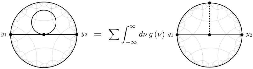
We develop a spectral approach to evaluate AdS loop diagrams, a central ingredient for which is the decomposition of bulk-to-bulk propagators G⁡(x1,x2)G\left(x_{1},x_{2}\right) into bi-tensorial AdS harmonic functions Ω⁡(x1,x2)\Omega\left(x_{1},x_{2}\right) [11, 12], which we depict as:

[Uncaptioned image].\includegraphics[scale={0.45}]{harmonic2.jpeg}. (1.1)

The factorisation of harmonic functions into bulk-to-boundary propagators integrated over the common boundary point [71]:

[Uncaptioned image],\includegraphics[scale={0.45}]{harmonic1.jpeg}, (1.2)

leads to the decomposition of loop diagrams into integrated products of higher point tree-level Witten diagrams. Upon evaluating the comparably simple tree-level Witten diagrams, the loop is reduced to the computation of well-known boundary conformal integrals [40] arising from the gluing of the tree-level bulk diagrams, and a spectral integral in the parameters ν\nu.

In this work, we detail this approach for two-point bubble and tadpole diagrams, which induce mass and wave-function renormalisations of the fields which already appear at tree-level. In this case, the task is reduced to the evaluation of tree-level three-point Witten diagrams (illustrated in figures 1(a) and 1(b)) which, via the sewing procedure shown in figure 1, give rise to the following three- and, ultimately, two-point conformal integrals:

I3pt​(y1,y2,y3)\displaystyle I_{\text{3pt}}\left(y_{1},y_{2},y_{3}\right) =∫dd​y[(y1−y)2]a1​[(y2−y)2]a2​[(y3−y)2]a3,a1+a2+a3=d,\displaystyle=\int\frac{d^{d}y}{\left[\left(y_{1}-y\right)^{2}\right]^{a_{1}}\left[\left(y_{2}-y\right)^{2}\right]^{a_{2}}\left[\left(y_{3}-y\right)^{2}\right]^{a_{3}}},\qquad a_{1}+a_{2}+a_{3}=d, (1.3a)
I2pt​(y1,y2)\displaystyle I_{\text{2pt}}\left(y_{1},y_{2}\right) =∫dd​y[(y1−y)2]a1​[(y2−y)2]a2,a1+a2=d,\displaystyle=\int\frac{d^{d}y}{\left[\left(y_{1}-y\right)^{2}\right]^{a_{1}}\left[\left(y_{2}-y\right)^{2}\right]^{a_{2}}},\qquad a_{1}+a_{2}=d, (1.3b)

whose evaluation we give in §A. The two-point integral (1.3b) is divergent, whose regularisation gives rise to the corrections to the wave function and the mass.

Refer to caption
((a))
Refer to caption
((b))
Figure 1:

For external totally symmetric fields of spin ss and tree-level mass mi2​R2=Δi​(Δi−d)−sm^{2}_{i}R^{2}=\Delta_{i}\left(\Delta_{i}-d\right)-s, the two-point one-loop diagrams ultimately take the form66 6 For tadpole diagrams, which have just a single bulk-to-bulk propagator, there is only one spectral integral while for bubble diagram (which instead involve two bulk-to-bulk propagators) there is a double integral as shown above. We emphasise that the presence of the divergent two-point conformal integral on the second line is universal. I.e. is generated by any one-loop process, both bubble and tadpole diagrams.

ℳ1-loop​(y1,y2)=∫−∞∞d​ν​dν¯​ℱ​(ν,ν¯)×𝖧12s(y122)(τ1+τ2−d)/2​∫dd​y[(y1−y)2]d/2+(Δ1−Δ2)/2​[(y2−y)2]d/2−(Δ1−Δ2)/2,{\cal M}^{\text{1-loop}}\left(y_{1},y_{2}\right)=\int^{\infty}_{-\infty}d\nu d{\bar{\nu}}{\cal F}\left(\nu,{\bar{\nu}}\right)\\ \times\frac{{\sf H}^{s}_{12}}{\left(y^{2}_{12}\right)^{(\tau_{1}+\tau_{2}-d)/2}}\int\frac{d^{d}y}{\left[\left(y_{1}-y\right)^{2}\right]^{d/2+(\Delta_{1}-\Delta_{2})/2}\left[\left(y_{2}-y\right)^{2}\right]^{d/2-(\Delta_{1}-\Delta_{2})/2}}, (1.4)

for some spectral function ℱ⁡(ν,ν¯){\cal F}\left(\nu,{\bar{\nu}}\right). We employ a variant of dimensional regularisation to evaluate the conformal integral on the second line,77 7 See §A.2 and §A.5 for a discussion on possible choices of regularisation, including at the level of the bulk harmonic function (3.9). which yields

I2pt1-loop​(y1,y2)\displaystyle I^{\text{1-loop}}_{\text{2pt}}\left(y_{1},y_{2}\right) =𝖧12s(y122)(τ1+τ2−d)/2​∫dd+ϵ​y[(y1−y)2]d/2+(Δ1−Δ2)/2​[(y2−y)2]d/2−(Δ1−Δ2)/2\displaystyle=\frac{{\sf H}^{s}_{12}}{\left(y^{2}_{12}\right)^{(\tau_{1}+\tau_{2}-d)/2}}\int\frac{d^{d+\epsilon}y}{\left[\left(y_{1}-y\right)^{2}\right]^{d/2+(\Delta_{1}-\Delta_{2})/2}\left[\left(y_{2}-y\right)^{2}\right]^{d/2-(\Delta_{1}-\Delta_{2})/2}}
=δΔ1,Δ2​πd+ϵ2Γ​(d2)2​𝖧12s(y122)(τ1+τ2−ϵ)/2​Γ​(ϵ2)2​Γ​(d−ϵ2)Γ⁡(ϵ)\displaystyle=\delta_{\Delta_{1},\Delta_{2}}\ \frac{\pi^{\frac{d+\epsilon}{2}}}{\Gamma(\tfrac{d}{2})^{2}}\frac{{\sf H}^{s}_{12}}{\left(y^{2}_{12}\right)^{(\tau_{1}+\tau_{2}-\epsilon)/2}}\frac{\Gamma\left(\frac{\epsilon}{2}\right)^{2}\Gamma\left(\frac{d-\epsilon}{2}\right)}{\Gamma(\epsilon)}
=δΔ1,Δ2​2​πd2Γ⁡(d2)​𝖧12s(y122)(τ1+τ2)/2​[2ϵ+log⁡(π)−ψ⁡(d2)+log⁡(y122)]+𝒪⁡(ϵ),\displaystyle=\delta_{\Delta_{1},\Delta_{2}}\ \frac{2\pi^{\frac{d}{2}}}{\Gamma(\tfrac{d}{2})}\frac{{\sf H}^{s}_{12}}{\left(y^{2}_{12}\right)^{(\tau_{1}+\tau_{2})/2}}\left[\frac{2}{\epsilon}+\log(\pi)-\psi\left(\tfrac{d}{2}\right)+\log\left(y^{2}_{12}\right)\right]+\mathcal{O}(\epsilon), (1.5)

where the constant piece generates the wave function renormalisation and the log term the mass correction.88 8 This can be understood from the expansion of the dual CFT two-point function ⟨𝒪Δ1,s​(y1)​𝒪Δ2,s​(y2)⟩\displaystyle\langle{\cal O}_{\Delta_{1},s}\left(y_{1}\right){\cal O}_{\Delta_{2},s}\left(y_{2}\right)\rangle =δΔ1​Δ2​C𝒪​𝖧12s(y122)τ1+γ\displaystyle=\delta_{\Delta_{1}\Delta_{2}}\,C_{{\cal O}}\frac{{\sf H}^{s}_{12}}{\left(y^{2}_{12}\right)^{\tau_{1}+\gamma}} =δΔ1​Δ2​C𝒪​𝖧12s(y122)τ1​e−γ​log⁡(y122)=δΔ1​Δ2​C𝒪​𝖧12s(y122)(τ1+τ2)/2​(1−γ​log⁡(y122)+…),\displaystyle=\delta_{\Delta_{1}\Delta_{2}}\,C_{{\cal O}}\frac{{\sf H}^{s}_{12}}{\left(y^{2}_{12}\right)^{\tau_{1}}}e^{-\gamma\log\left(y^{2}_{12}\right)}=\delta_{\Delta_{1}\Delta_{2}}\,C_{{\cal O}}\frac{{\sf H}^{s}_{12}}{\left(y^{2}_{12}\right)^{(\tau_{1}+\tau_{2})/2}}\left(1-\gamma\log\left(y^{2}_{12}\right)+...\right), where we see that the anomalous dimension, which is related to the corrected bulk mass via m2​R2=(Δ+γ)​(Δ+γ−d)−sm^{2}R^{2}=\left(\Delta+\gamma\right)\left(\Delta+\gamma-d\right)-s, is the coefficient of the log term. Combining (1.5) with (1.4) thus gives the anomalous dimension in the spectral form

γ∼−δΔ1​Δ2∫−∞∞dνdν¯ℱ(ν,ν¯).\displaystyle\gamma\sim-\delta_{\Delta_{1}\Delta_{2}}\int^{\infty}_{-\infty}d\nu d{\bar{\nu}}\,{\cal F}\left(\nu,{\bar{\nu}}\right). (1.6)

The above procedure is not only computationally convenient, but also turns out to disentangle UV and IR bulk divergences. It is indeed easy to see by inspection that the spectral integrals will diverge for large values of the spectral parameter, which therefore should be considered a UV divergence. Such UV divergences translate into divergent anomalous dimensions which require regularisation. While UV finite theories will lead to well-defined predictions for the anomalous dimensions, UV divergent theories will require some subtraction scheme to extract the anomalous dimensions. In the latter case, in this paper we shall use a minimal subtraction scheme. The boundary integrals instead are by construction IR effects, which correspond to short distance singularities from the perspective of the boundary CFT. The fact that it is possible to generate anomalous dimensions even when no UV counter-term is required is a peculiarity of the IR structure of AdS space [72].

All of the above spectral integrals will be of the form of Mellin-Barnes integrals, which define generalisations of hypergeometric functions:

Hp,qm,n​(z)=∫∏j=1mΓ⁡(bj−i​ν)​∏j=1nΓ⁡(1−aj+i​ν)∏j=n+1pΓ⁡(aj−i​ν)​∏j=m+1qΓ⁡(1−bj+i​ν)​zi​ν​𝑑ν.H^{m,n}_{p,q}\left(z\right)=\int\frac{\prod^{m}_{j=1}\Gamma\left(b_{j}-i\nu\right)\prod^{n}_{j=1}\Gamma\left(1-a_{j}+i\nu\right)}{\prod^{p}_{j=n+1}\Gamma\left(a_{j}-i\nu\right)\prod^{q}_{j=m+1}\Gamma\left(1-b_{j}+i\nu\right)}z^{i\nu}d\nu. (1.7)

The latter, for z=±1z=\pm 1 can be expressed in terms of sums of generalised hypergeometric functions of argument ±1\pm 1 and can be evaluated by the Gauss hypergeometric formula. Once the anomalous dimension is extracted in terms of a spectral integral the problem of evaluating the loop diagram is drastically simplified and can be solved either analytically (when possible) or numerically. While in this work we focus on some relevant examples, we leave for the future the problem of developing a systematic analytic/numeric method to evaluate the above integrals in general in the case of multiple spectral integrals.

1.2 Notation, conventions and ambient space

In this work we consider tensor fields in Euclidean anti-de Sitter (AdSd+1) space where, unless specified, the boundary dimension dd is taken to be general. We employ an operator notation to package the tensor indices (for a review see e.g. [66], whose conventions we adopt throughout), where a totally symmetric rank-ss bulk field φμ1​…​μs\varphi_{\mu_{1}...\mu_{s}} represented by the generating function

φμ1​…​μs​(x)→φs​(x,u)=1s!​φμ1​…​μs​(x)​uμ1​…​uμs,\varphi_{\mu_{1}...\mu_{s}}\left(x\right)\>\rightarrow\>\varphi_{s}\left(x;u\right)=\frac{1}{s!}\varphi_{\mu_{1}...\mu_{s}}\left(x\right)u^{\mu_{1}}...u^{\mu_{s}}, (1.8)

where we introduced the (d+1)\left(d+1\right)-dimensional constant auxiliary vector uμu^{\mu}. The covariant derivative gets modified when acting on fields expressed in the generating function form (1.8):

∇μ→∇μ+ωμa​b​ua​∂∂ub,\nabla_{\mu}\;\rightarrow\;\nabla_{\mu}+\omega^{ab}_{\mu}u_{a}\frac{\partial}{\partial u^{b}}, (1.9)

where ωμa​b\omega^{ab}_{\mu} is the spin connection and ua=eμa​(x)​uμu^{a}=e^{a}_{\mu}\left(x\right)u^{\mu} with vielbein eμa​(x)e^{a}_{\mu}\left(x\right).

One particular virtue of this notation is that tensor operations become an operator calculus, which significantly simplifies manipulations. For instance, the contraction:

φμ1​…​μs(x)φμ1​…​μs(x)=s!φs(x;∂u)φ(x;u),\varphi_{\mu_{1}...\mu_{s}}\left(x\right)\varphi^{\mu_{1}...\mu_{s}}\left(x\right)=s!\,\varphi_{s}\left(x;\partial_{u}\right)\varphi\left(x;u\right), (1.10)

and the operations: divergence, symmetrised gradient, box, symmetrised metric, trace and spin are represented by the following operators:

divergence: ∇⋅∂u,\displaystyle\nabla\cdot\partial_{u}, sym. gradient: u⋅∇,\displaystyle u\cdot\nabla, box: □,\displaystyle\Box, (1.11)
sym. metric: u2,\displaystyle u^{2}, trace: ∂u2,\displaystyle\partial_{u}^{2}, spin: u⋅∂u.\displaystyle u\cdot\partial_{u}.

Likewise, operators of non-trivial spin living on the conformal boundary of AdSd+1 can be expressed in generating function notation. A totally symmetric spin-ss operator 𝒪i1​…​is{\cal O}_{i_{1}...i_{s}} at the boundary point yiy^{i}, i=1,…,di=1,...,d, is represented as

𝒪i1​…​is​(y)→𝒪s​(y,z)=𝒪i1​…​is​(y)​zi1​…​zis,{\cal O}_{i_{1}...i_{s}}\left(y\right)\>\rightarrow\>{\cal O}_{s}\left(y;z\right)={\cal O}_{i_{1}...i_{s}}\left(y\right)z^{i_{1}}...z^{i_{s}}, (1.12)

with the null auxiliary vector z2=0z^{2}=0 enforcing the tracelessness condition. The operator calculus is slightly modified for traceless tensors, since one must instead replace the partial derivative ∂z\partial_{z} with the Thomas derivative [73]:99 9 In the CFT literature this is sometimes referred to as the Todorov differential operator [74]. The normalisation of the latter is obtained from (1.13) by multiplying by the operator d−2+2z⋅∂zd-2+2z\cdot\partial_{z}, and recalling that z⋅∂zz\cdot\partial_{z} gives the spin of the operator being acted on.

∂^zi=∂zi−1d−2+2z⋅∂zzi∂2z,{\hat{\partial}}_{z^{i}}=\partial_{z^{i}}-\frac{1}{d-2+2z\cdot\partial_{z}}z_{i}\partial^{2}_{z}, (1.13)

that preserves the condition z2=0z^{2}=0. For example,

𝒪i1,…,is​(y)​𝒪i1,…,is​(y)=s!​𝒪s​(y,∂^z)​𝒪s​(y,z).{\cal O}_{i_{1},...,i_{s}}\left(y\right){\cal O}^{i_{1},...,i_{s}}\left(y\right)=s!\,{\cal O}_{s}(y;{\hat{\partial}}_{z}){\cal O}_{s}\left(y;z\right). (1.14)

Ambient space

The ambient space formalism is an indispensable tool in AdS and CFT, which simplifies computations considerably by making the S​O​(1,d+1)SO\left(1,d+1\right) symmetry manifest. We employ this formalism throughout, and briefly review the pertinent details here. For further details see e.g. [75, 76, 77, 78, 66].

A perspective first considered by Dirac [79], in the ambient space formalism one regards the AdSd+1 space as the co-dimension one hyper-surface

X2+R2=0,X^{2}+R^{2}=0, (1.15)

in an ambient flat space-time parameterised by Cartesian co-ordinates XAX^{A} where A=0,1,..,d+1A=0,1,..,d+1 and metric ηA​B=diag(−++…+)\eta_{AB}=\text{diag}\left(-++...+\right) to describe Euclidean AdS.1010 10 In contrast Lorentzian AdS would require the conformal signature: ηA​B=diag(−++…+−)\eta_{AB}=\text{diag}\left(-++...+-\right).

A smooth irreducible s​o​(1,d+1)so\left(1,d+1\right)-tensor field φμ1​…​μs​(x)\varphi_{\mu_{1}...\mu_{s}}\left(x\right) of mass

m2​R2=Δ⁡(Δ−d)−s,m^{2}R^{2}=\Delta\left(\Delta-d\right)-s, (1.16)

is represented uniquely in the ambient space by a field φA1​…​As​(X)\varphi_{A_{1}...A_{s}}\left(X\right) of the same rank subject to the following constraints [80]:

  • •

    Tangentiality to surfaces of constant ρ=−X2\rho=\sqrt{-X^{2}}:

    XAiφA1​…​Ai​…​As=0,i=1,…,s.X^{A_{i}}\varphi_{A_{1}...A_{i}...A_{s}}=0,\quad i=1,...,s. (1.17)

    Explicitly, one can apply the projection operator:

    𝒫AB=δAB−XA​XBX2,{\cal P}_{A}^{B}=\delta^{B}_{A}-\frac{X_{A}X^{B}}{X^{2}}, (1.18)

    which acts on ambient tensors as

    (𝒫​φ)A1​…​As:=𝒫A1B1​…​𝒫AsBs​φB1​…​Bs,XAi​(𝒫​φ)B1​…​Bi​…​Bs=0\left({\cal P}\varphi\right)_{A_{1}...A_{s}}:={\cal P}_{A_{1}}^{B_{1}}...{\cal P}_{A_{s}}^{B_{s}}\varphi_{B_{1}...B_{s}},\qquad X^{A_{i}}\left({\cal P}\varphi\right)_{B_{1}...B_{i}...B_{s}}=0 (1.19)
  • •

    The homogeneity condition:

    (X⋅∂X+μ)φs(X,U)=0,i.e.φs(λX,U)=λ−μφs(X,U),\left(X\cdot\partial_{X}+\mu\right)\varphi_{s}\left(X,U\right)=0,\quad\text{i.e.}\quad\varphi_{s}\left(\lambda X,U\right)=\lambda^{-\mu}\varphi_{s}\left(X,U\right), (1.20)

    where we are free to choose either μ=Δ\mu=\Delta or μ=d−Δ\mu=d-\Delta. In this work we take μ=Δ\mu=\Delta. This fixes how the ambient representative extends away from the AdS manifold, in the radial direction ρ=−X2\rho=\sqrt{-X^{2}}.

The above conditions ensure that the ambient uplift of fields that live on the AdS manifold is well-defined and one-to-one.

This discussion also extends to differential operators. For instance, the ambient representative of the Levi-Civita connection ∇μ\nabla_{\mu} on AdSd+1 is given by [81, 82]:

∇A=𝒫BA∂∂XB,X⋅∇=0.\nabla_{A}={\cal P}^{B}_{A}\frac{\partial}{\partial X^{B}},\qquad X\cdot\nabla=0. (1.21)

Crucially, this must act on ambient tensors that are tangent, otherwise extra terms may be introduced which are not killed by the projector acting on the LHS of (1.21). The proper action of (1.21) should thus be regarded as:

∇=𝒫∘∂∘𝒫.\nabla={\cal P}\circ\partial\circ{\cal P}. (1.22)

For example:

∇BTA1​…​Ar=𝒫BC​𝒫A1C1​…​𝒫ArCr​∂∂XC​(𝒫​T)C1​…​Cr,\nabla_{B}T_{A_{1}...A_{r}}={\cal P}^{C}_{B}{\cal P}^{C_{1}}_{A_{1}}...{\cal P}^{C_{r}}_{A_{r}}\frac{\partial}{\partial X^{C}}\left({\cal P}T\right)_{C_{1}...C_{r}}, (1.23)

for some ambient tensor TA1​…​Ar​(X)T_{A_{1}...A_{r}}\left(X\right).

The operator notation for tensor fields introduced in the previous section can also be extended to ambient space. We have:

φA1..As​(X)→φs​(X,U)=1s!​φA1..As​(X)​UA1​…​UAs,\varphi_{A_{1}..A_{s}}\left(X\right)\>\rightarrow\>\varphi_{s}\left(X;U\right)=\frac{1}{s!}\varphi_{A_{1}..A_{s}}\left(X\right)U^{A_{1}}...U^{A_{s}}, (1.24)

with constant ambient auxiliary vector UAU^{A}. Like for the intrinsic case (1.9), the covariant derivative (1.21) also gets modified in the operator formalism [77]:

∇A→∇A−XBX2​ΣA​B,\nabla_{A}\>\rightarrow\>\nabla_{A}-\frac{X^{B}}{X^{2}}\Sigma_{AB}, (1.25)

where

ΣA​B=UA​∂∂UB−UB​∂∂UA.\Sigma_{AB}=U_{A}\frac{\partial}{\partial U^{B}}-U_{B}\frac{\partial}{\partial U^{A}}. (1.26)

The ambient formalism extends to the boundary of AdS [83, 79, 80, 84, 85, 86, 78]. Towards the boundary, the hyperboloid (1.15) asymptotes to the light-cone. This limit does not give rise to a well-defined boundary metric, but a finite limit can be obtained by considering a projective cone of light-rays:

PA≡ϵ​XA,ϵ→0.P^{A}\equiv\epsilon X^{A},\quad\epsilon\rightarrow 0. (1.27)

Since X2X^{2} is fixed, these null co-ordinates satisfy:

P2=0,P≅λ​P,λ≠0,P^{2}=0,\qquad P\cong\lambda P,\qquad\lambda\neq 0, (1.28)

and are identified with the AdS boundary. For example, for Euclidean AdS in Poincaré co-ordinates xμ=(z,yi)x^{\mu}=\left(z,y^{i}\right), we have:

X0​(x)\displaystyle X^{0}\left(x\right) =R​z2+y2+12​z\displaystyle=R\frac{z^{2}+y^{2}+1}{2z} (1.29a)
Xd+1​(x)\displaystyle X^{d+1}\left(x\right) =R​1−z2−y22​z\displaystyle=R\frac{1-z^{2}-y^{2}}{2z} (1.29b)
Xi​(x)\displaystyle X^{i}\left(x\right) =R​yiz,\displaystyle=\frac{Ry^{i}}{z}, (1.29c)

and the boundary points are parameterised by the Poincaré section:

P0​(y)=12​(1+y2),Pd+1​(y)=12​(1−y2),Pi​(y)=yi.P^{0}\left(y\right)=\frac{1}{2}\left(1+y^{2}\right),\quad P^{d+1}\left(y\right)=\frac{1}{2}\left(1-y^{2}\right),\quad P^{i}\left(y\right)=y^{i}. (1.30)

The ambient representative fA1​…​As​(P)f_{A_{1}...A_{s}}\left(P\right) of a symmetric spin-ss boundary field fi1​…​is​(y)f_{i_{1}...i_{s}}\left(y\right) of scaling dimension Δ\Delta is traceless with respect to the ambient metric1111 11 It is not difficult to see that this follows from the tracelessness of fi1​…​isf_{i_{1}...i_{s}}.

ηA​B​fA1​…​As=0\eta^{AB}f_{A_{1}...A_{s}}=0 (1.31)

and scales as

fA1​…​As​(λ​P)=λ−Δ​fA1​…​As​(P),λ>0.f_{A_{1}...A_{s}}\left(\lambda P\right)=\lambda^{-\Delta}f_{A_{1}...A_{s}}\left(P\right),\qquad\lambda>0. (1.32)

Like for the ambient description of bulk fields, we require that fA1​…​Asf_{A_{1}...A_{s}} is tangent to the light-cone:

PA1​fA1​…​As​(P)=0.P^{A_{1}}f_{A_{1}...A_{s}}\left(P\right)=0. (1.33)

However, since P2=0P^{2}=0, there is an extra redundancy

fA1​…​As​(P)→fA1​…​As​(P)+P(A1CLOSE​ΛOPENA2​…​As),\displaystyle\hskip 99.58464ptf_{A_{1}...A_{s}}(P)\rightarrow f_{A_{1}...A_{s}}(P)+P_{\left(A_{1}\right.}\Lambda_{\left.A_{2}...A_{s}\right)}, (1.34)
PA1​ΛA1​…​As−1=0,ΛA1​…​As−1​(λ​P)=λ−(Δ+1)​ΛA1​…​As−1​(P),ηA1​A2​ΛA1​…​As−1=0,\displaystyle P^{A_{1}}\Lambda_{A_{1}...A_{s-1}}=0,\quad\Lambda_{A_{1}...A_{s-1}}(\lambda P)=\lambda^{-(\Delta+1)}\Lambda_{A_{1}...A_{s-1}}(P),\quad\eta^{A_{1}A_{2}}\Lambda_{A_{1}...A_{s-1}}=0, (1.35)

which, together with (1.33), eliminates the extra two degrees of freedom per index of fA1​…​Asf_{A_{1}...A_{s}}.

Likewise the operator formalism extends to ambient boundary fields, where we have:

fA1​…​As​(P)→fs​(P,Z)=1s!​fA1​…​As​(P)​ZA1​…​ZAs,Z2=0,P⋅Z=0,f_{A_{1}...A_{s}}\left(P\right)\>\rightarrow\>f_{s}\left(P;Z\right)=\frac{1}{s!}f_{A_{1}...A_{s}}\left(P\right)Z^{A_{1}}...Z^{A_{s}},\quad Z^{2}=0,\quad P\cdot Z=0, (1.36)

where as usual Z2=0Z^{2}=0 enforces the traceless condition (1.31) and it is useful to impose the new constraint P⋅Z=0P\cdot Z=0 that takes care of tangentiality to the light-cone (1.33).

2 Scalar diagrams

For ease of illustration, we first consider two-point one-loop diagrams involving only scalar fields. We review the basic ingredients below before giving some concrete applications in §2.1 and §2.3.

Bulk-to-boundary propagators take a very simple form in ambient space. See §1.2 for a review of the ambient space formalism. For a scalar of mass m2​R2=Δ⁡(Δ−d)m^{2}R^{2}=\Delta\left(\Delta-d\right), the bulk-to-boundary propagator1212 12 In the limit we used Poincaré co-ordinates (1.29a) with xμ=(z,y¯i)x^{\mu}=\left(z,{\bar{y}}^{i}\right), where the y¯i{\bar{y}}^{i} with i=1,…,di=1,...,d parameterise the boundary directions.

(−□+m2)​KΔ,0​(x,y)=0,limz→0(zΔ−d​KΔ,0​(z,y¯,y))=12​Δ−d​δd​(y−y¯),\left(-\Box+m^{2}\right)K_{\Delta,0}\left(x;y\right)=0,\qquad\lim_{z\rightarrow 0}\left(z^{\Delta-d}K_{\Delta,0}\left(z,{\bar{y}};y\right)\right)=\frac{1}{2\Delta-d}\delta^{d}\left(y-{\bar{y}}\right), (2.1)

is given by the contraction:

KΔ,0​(X⁡(x),P⁡(y))=CΔ,0(−2X⋅P)Δ,K_{\Delta,0}\left(X\left(x\right);P\left(y\right)\right)=\frac{C_{\Delta,0}}{\left(-2X\cdot P\right)^{\Delta}}, (2.2)

with normalisation:

CΔ,0=Γ⁡(Δ)2​πd/2​Γ​(Δ+1−d2).C_{\Delta,0}=\frac{\Gamma\left(\Delta\right)}{2\pi^{d/2}\Gamma\left(\Delta+1-\tfrac{d}{2}\right)}. (2.3)

We employ the spectral representation of the bulk-to-bulk propagators, which for scalar fields with Δ>d2\Delta>\frac{d}{2} is given by1313 13 The case Δ<d2\Delta<\frac{d}{2} requires a slight modification of the propagator, but the general approach for evaluating loop diagrams is unchanged. This is explained later on in §4.2.1.

GΔ,0​(x1,x2)\displaystyle G_{\Delta,0}\left(x_{1};x_{2}\right) =∫−∞∞d​ν[ν2+(Δ−d2)2]​Ων,0​(x1,x2),\displaystyle=\int^{\infty}_{-\infty}\frac{d\nu}{\left[\nu^{2}+\left(\Delta-\frac{d}{2}\right)^{2}\right]}\Omega_{\nu,0}\left(x_{1},x_{2}\right), (2.4)

where Ων,0\Omega_{\nu,0} is a spin 00 bi-tensorial harmonic function with equation of motion

(□1+(d2)2+ν2)​Ων,0​(x1,x2)=0,\left(\Box_{1}+\left(\tfrac{d}{2}\right)^{2}+\nu^{2}\right)\Omega_{\nu,0}\left(x_{1},x_{2}\right)=0, (2.5)

where the subscript i on differential operators signifies that the derivative is being taken with respect to xix_{i}. As is illustrated in figure 1, the factorisation

Ων,0​(x1,x2)=ν2π​∫∂AdSdd​y​Kd2+i​ν​.0​(x1,y)​Kd2−i​ν,0​(x2,y),\Omega_{\nu,0}\left(x_{1},x_{2}\right)=\frac{\nu^{2}}{\pi}\int_{\partial\text{AdS}}d^{d}y\,K_{\frac{d}{2}+i\nu.0}\left(x_{1};y\right)K_{\frac{d}{2}-i\nu,0}\left(x_{2};y\right), (2.6)

of harmonic functions into bulk-to-boundary propagators (2.2) re-expresses two-point one-loop diagrams in terms of conformal integrals of tree-level three-point Witten diagrams. For diagrams involving only scalar fields, the three-point Witten diagrams are those generated by the basic vertex1414 14 Note that this vertex is the unique cubic vertex of scalars on-shell.

𝒱(3)=ϕ1​ϕ2​ϕ3,{\cal V}^{\left(3\right)}=\phi_{1}\phi_{2}\phi_{3}, (2.7)

of scalars ϕi\phi_{i} of some mass mi2​R2=Δi​(Δi−d)m^{2}_{i}R^{2}=\Delta_{i}\left(\Delta_{i}-d\right). The tree-level amplitude generated by (2.7) is well known [5], and given in the ambient formalism (see §1.2) by

ℳΔ1,Δ2,Δ33pt tree​(P1,P2,P3)=𝖡⁡(Δ1,Δ2,Δ3,0)P13Δ1+Δ3−Δ22​P23Δ2+Δ3−Δ12​P12Δ1+Δ2−Δ32,{\cal M}^{\text{3pt tree}}_{\Delta_{1},\Delta_{2},\Delta_{3}}\left(P_{1},P_{2},P_{3}\right)=\frac{{\sf B}\left(\Delta_{1},\Delta_{2},\Delta_{3};0\right)}{P^{\frac{\Delta_{1}+\Delta_{3}-\Delta_{2}}{2}}_{13}P^{\frac{\Delta_{2}+\Delta_{3}-\Delta_{1}}{2}}_{23}P^{\frac{\Delta_{1}+\Delta_{2}-\Delta_{3}}{2}}_{12}}, (2.8)

where Pi​j=−2Pi⋅PjP_{ij}=-2P_{i}\cdot P_{j} and

𝖡⁡(Δ1,Δ2,Δ3,0)=12​πd2​Γ​(−d+∑i=13Δi2)​CΔ1,0​CΔ2,0​CΔ3,0×Γ⁡(Δ1+Δ2−Δ32)​Γ​(Δ1+Δ3−Δ22)​Γ​(Δ2+Δ3−Δ12)Γ⁡(Δ1)​Γ​(Δ2)​Γ​(Δ3).{\sf B}\left(\Delta_{1},\Delta_{2},\Delta_{3};0\right)=\;\frac{1}{2}\pi^{\frac{d}{2}}\Gamma\left(\frac{-d+\sum\nolimits^{3}_{i=1}\Delta_{i}}{2}\right)C_{\Delta_{1},0}C_{\Delta_{2},0}C_{\Delta_{3},0}\\ \times\frac{\Gamma\left(\frac{\Delta_{1}+\Delta_{2}-\Delta_{3}}{2}\right)\Gamma\left(\frac{\Delta_{1}+\Delta_{3}-\Delta_{2}}{2}\right)\Gamma\left(\frac{\Delta_{2}+\Delta_{3}-\Delta_{1}}{2}\right)}{\Gamma\left(\Delta_{1}\right)\Gamma\left(\Delta_{2}\right)\Gamma\left(\Delta_{3}\right)}. (2.9)

The CΔi,0C_{\Delta_{i},0} come from the normalisation (2.3) of the bulk-to-boundary propagator.

In §2.1 we use this approach to evaluate the two-point one-loop bubble diagram in ϕ3\phi^{3} theory. In §2.3 we move on to tadpole diagrams, showing in §2.3.1 how they are evaluated in ϕ4\phi^{4} theory. We extend the latter result to arbitrary derivative quartic self-interactions in §2.3.3.

2.1 2pt bubble

Refer to caption
Figure 2: Scalar one-loop bubble diagram generated by the cubic couplings (2.10).

We consider the two-point one-loop bubble illustrated in figure 2, which is generated by the following cubic couplings:1515 15 In this subsection we drop symmetry factors associated to indistinguishable external legs. In the case of indistinguishable scalar fields, the corresponding symmetry factor is S=12S=\frac{1}{2}.

𝒱1(3)=g​ϕ1​ϕ​ϕ¯,𝒱2(3)=g¯​ϕ2​ϕ​ϕ¯,{\cal V}^{(3)}_{1}=g\,\phi_{1}\phi{\bar{\phi}},\qquad{\cal V}^{(3)}_{2}={\bar{g}}\,\phi_{2}\phi{\bar{\phi}}, (2.10)

for arbitrary coupling constants gg and g¯{\bar{g}}. The diagram is given by evaluating the bulk integrals

ℳ2pt bubble​(P1,P2)=g​g¯​∫AdSd​X1​d​X2​KΔ1,0​(X1,P1)​GΔ,0​(X1,X2)​GΔ¯,0​(X1,X2)​KΔ2,0​(X2,P2).{\cal M}^{\text{2pt bubble}}\left(P_{1},P_{2}\right)\\ =g{\bar{g}}\int_{\text{AdS}}dX_{1}dX_{2}\,K_{\Delta_{1},0}\left(X_{1};P_{1}\right)G_{\Delta,0}\left(X_{1};X_{2}\right)G_{{\bar{\Delta}},0}\left(X_{1};X_{2}\right)K_{\Delta_{2},0}\left(X_{2};P_{2}\right). (2.11)

The spectral representation (2.4) of the scalar bulk-to-bulk propagators expresses the diagram in terms of two tree-level three-point Witten diagrams (2.8), sewn together by their common boundary points (see figure 1(a)):

ℳ2pt bubble​(P1,P2)=g​g¯​∫−∞∞ν2​ν¯2​d​ν​d​ν¯π2​[ν2+(Δ−d2)2]​[ν¯2+(Δ¯−d2)2]×∫∂AdSd​P​dP¯​ℳΔ1,d2+i​ν,d2+i​ν¯3pt tree​(P1,P,P¯)​ℳΔ2,d2−i​ν,d2−i​ν¯3pt tree​(P2,P,P¯).{\cal M}^{\text{2pt bubble}}\left(P_{1},P_{2}\right)=g{\bar{g}}\int^{\infty}_{-\infty}\frac{\nu^{2}{\bar{\nu}}^{2}d\nu d{\bar{\nu}}}{\pi^{2}[\nu^{2}+(\Delta-\frac{d}{2})^{2}][{\bar{\nu}}^{2}+({\bar{\Delta}}-\frac{d}{2})^{2}]}\\ \times\int_{\partial\text{AdS}}dPd{\bar{P}}\,{\cal M}_{\Delta_{1},\,\frac{d}{2}+i\nu,\,\frac{d}{2}+i{\bar{\nu}}}^{\text{3pt tree}}(P_{1},P,{\bar{P}})\,{\cal M}_{\Delta_{2},\,\frac{d}{2}-i\nu,\,\frac{d}{2}-i{\bar{\nu}}}^{\text{3pt tree}}(P_{2},P,{\bar{P}}). (2.12)

The integrals in PP and P¯\bar{P} are both of the three-point conformal type (1.3a). Performing first, say, the integration over P¯\bar{P} leaves the two-point conformal integral (1.3b):

ℳ2pt bubble​(P1,P2)=g​g¯64​πd+82​CΔ1,0​CΔ2,0Γ⁡(Δ1)​Γ​(Δ2)​Γ⁡(Δ1+Δ2−d2)Γ⁡(d−Δ1+Δ22)​∫−∞∞d​ν​dν¯​ℱ2pt bubble​(ν,ν¯)×P12d−Δ1−Δ22​∫d​P(−2P1⋅P)12​(d+Δ1−Δ2)(−2P2⋅P)12​(d+Δ2−Δ1)⏟=I2pt1-loop​(y1,y2)​(1.5){\cal M}^{\text{2pt bubble}}\left(P_{1},P_{2}\right)=\frac{g{\bar{g}}}{64\pi^{\frac{d+8}{2}}}\frac{C_{\Delta_{1},0}C_{\Delta_{2},0}}{\Gamma\left(\Delta_{1}\right)\Gamma\left(\Delta_{2}\right)}\frac{\Gamma\left(\frac{\Delta_{1}+\Delta_{2}-d}{2}\right)}{\Gamma\left(d-\frac{\Delta_{1}+\Delta_{2}}{2}\right)}\int^{\infty}_{-\infty}d\nu d{\bar{\nu}}\,{\cal F}^{\text{2pt bubble}}\left(\nu,{\bar{\nu}}\right)\\ \times\underbrace{P_{12}^{\frac{d-\Delta_{1}-\Delta_{2}}{2}}\int\frac{dP}{\left(-2P_{1}\cdot P\right)^{\frac{1}{2}\left(d+\Delta_{1}-\Delta_{2}\right)}\left(-2P_{2}\cdot P\right)^{\frac{1}{2}\left(d+\Delta_{2}-\Delta_{1}\right)}}}_{=I^{\text{1-loop}}_{\text{2pt}}\left(y_{1},y_{2}\right)\ \eqref{M12}} (2.13)

where

ℱ2pt bubble​(ν,ν¯)=ν​ν¯​sinh⁡(π​ν)​sinh⁡(π​ν¯)[(d2−Δ¯)2+ν¯2]​[(d2−Δ)2+ν2]×Γ⁡(d−Δ1−i⁡(ν−ν¯)2)​Γ​(d−Δ1+i⁡(ν+ν¯)2)​Γ​(Δ1−i⁡(ν−ν¯)2)​Γ​(Δ1+i⁡(ν+ν¯)2)×Γ⁡(d−Δ2+i⁡(ν−ν¯)2)​Γ​(d−Δ2−i⁡(ν+ν¯)2)​Γ​(Δ2+i⁡(ν−ν¯)2)​Γ​(Δ2−i⁡(ν+ν¯)2).{\cal F}^{\text{2pt bubble}}\left(\nu,{\bar{\nu}}\right)=\frac{\nu{\bar{\nu}}\sinh(\pi\nu)\sinh(\pi{\bar{\nu}})}{\left[(\tfrac{d}{2}-{\bar{\Delta}})^{2}+{\bar{\nu}}^{2}\right]\left[(\tfrac{d}{2}-\Delta)^{2}+\nu^{2}\right]}\\ \times\Gamma\left(\tfrac{d-\Delta_{1}-i(\nu-{\bar{\nu}})}{2}\right)\Gamma\left(\tfrac{d-\Delta_{1}+i(\nu+{\bar{\nu}})}{2}\right)\Gamma\left(\tfrac{\Delta_{1}-i(\nu-{\bar{\nu}})}{2}\right)\Gamma\left(\tfrac{\Delta_{1}+i(\nu+{\bar{\nu}})}{2}\right)\\ \times\Gamma\left(\tfrac{d-\Delta_{2}+i(\nu-{\bar{\nu}})}{2}\right)\Gamma\left(\tfrac{d-\Delta_{2}-i(\nu+{\bar{\nu}})}{2}\right)\Gamma\left(\tfrac{\Delta_{2}+i(\nu-{\bar{\nu}})}{2}\right)\Gamma\left(\tfrac{\Delta_{2}-i(\nu+{\bar{\nu}})}{2}\right)\,. (2.14)

Focusing on the log⁡(y122)\log(y_{12}^{2}) contribution, we can thus extract the leading correction to the anomalous dimension as the following spectral integral:

γ=−g​g¯​δΔ1​Δ2​Γ⁡(Δ1+Δ2−d2)64​πd+82​Γ​(d2)​Γ​(d−Δ1+Δ22)​1Γ⁡(Δ1)​Γ​(−d2+Δ1+1)​Γ⁡(Δ2)​Γ​(−d2+Δ2+1)×∫−∞∞d​ν​dν¯​ℱ2pt bubble​(ν,ν¯)\gamma=-g{\bar{g}}\,\delta_{\Delta_{1}\Delta_{2}}\frac{\Gamma\left(\frac{\Delta_{1}+\Delta_{2}-d}{2}\right)}{64\pi^{\frac{d+8}{2}}\Gamma\left(\frac{d}{2}\right)\Gamma\left(d-\frac{\Delta_{1}+\Delta_{2}}{2}\right)}\frac{1}{\sqrt{\Gamma(\Delta_{1})\Gamma\left(-\frac{d}{2}+\Delta_{1}+1\right)}\sqrt{\Gamma(\Delta_{2})\Gamma\left(-\frac{d}{2}+\Delta_{2}+1\right)}}\\ \times\int^{\infty}_{-\infty}d\nu d{\bar{\nu}}\,{\cal F}^{\text{2pt bubble}}\left(\nu,{\bar{\nu}}\right) (2.15)

In the following sections we first demonstrate how the spectral integrals may be evaluated in some simple examples, and in §2.2 we detail a general analytic approach based on summing over residues. In §3.3 we also discuss the pole structure of the spectral function (2.14).

2.1.1 Conformally coupled scalar (Δ=2\Delta=2) in AdS4

The simplest case is that of the self-coupling of a conformally coupled scalar in AdS4, i.e.:

𝒱1(3)=𝒱2(3)=g3!​ϕ3,{\cal V}^{(3)}_{1}={\cal V}^{(3)}_{2}=\frac{g}{3!}\,\phi^{3}, (2.16)

with Δ=2\Delta=2. In this section all formulas below will include the corresponding symmetry factor S=12S=\tfrac{1}{2}.

In this case the spectral representation of the anomalous dimension (2.15) is:

γ=−Sg2∫ℝ2ν​ν¯​(ν−ν¯)​(ν+ν¯)​sinh⁡(π​ν)​sinh⁡(π​ν¯)​csch​(π⁡(ν−ν¯))​csch​(π⁡(ν+ν¯))π2​(4​ν2+1)​(4​ν¯2+1).\gamma=-S\,g^{2}\int_{\mathbb{R}^{2}}\frac{\nu\bar{\nu}(\nu-\bar{\nu})(\nu+\bar{\nu})\sinh(\pi\nu)\sinh(\pi\bar{\nu})\text{csch}(\pi(\nu-\bar{\nu}))\text{csch}(\pi(\nu+\bar{\nu}))}{\pi^{2}\left(4\nu^{2}+1\right)\left(4\bar{\nu}^{2}+1\right)}\,. (2.17)

To study the above integral it is convenient to make the following change of variables:

x\displaystyle x =ν+ν¯,\displaystyle=\nu+{\bar{\nu}}\,, y\displaystyle y =ν−ν¯,\displaystyle=\nu-{\bar{\nu}}\,, (2.18)

through which the (2.17) becomes:

γ=−S​g22​π2∫0∞dx∫0∞dyx​y​(x2−y2)​csch​(π​x)​csch​(π​y)​sinh⁡(π2​(x−y))​sinh⁡(π2​(x+y))((y−x)2+1)​((x+y)2+1)⏟I⁡(x,y),\gamma=-\frac{S\,g^{2}}{2\pi^{2}}\int_{0}^{\infty}dx\int_{0}^{\infty}dy\,\underbrace{\frac{xy\left(x^{2}-y^{2}\right)\text{csch}(\pi x)\text{csch}(\pi y)\sinh\left(\frac{\pi}{2}(x-y)\right)\sinh\left(\frac{\pi}{2}(x+y)\right)}{\left((y-x)^{2}+1\right)\left((x+y)^{2}+1\right)}}_{I(x,y)}\,, (2.19)

where we have used the symmetries of the integral to restrict the region of integration to the first quadrant of the plane. In the above form it is straightforward to identify the singularity of the integral which arises for x→∞x\to\infty or y→∞y\to\infty from the asymptotic behavior the integrand:

I⁡(x,y)\displaystyle I(x,y) ∼1x+𝒪(1x3)yfixed,\displaystyle\sim\frac{1}{x}+\mathcal{O}\left(\frac{1}{x^{3}}\right)\qquad y\ \text{fixed}\,, (2.20)
I⁡(x,y)\displaystyle I(x,y) ∼1y+𝒪(1y3)xfixed.\displaystyle\sim\frac{1}{y}+\mathcal{O}\left(\frac{1}{y^{3}}\right)\qquad x\ \text{fixed}\,. (2.21)

A standard way to regularise integrals of the above type is to use ζ\zeta-function regularisation, which entails introducing a parameter μ\mu:

γ(μ)=−S​g22​π2∫0∞dx∫0∞dyx​y​(x2−y2)​csch​(π​x)​csch​(π​y)​sinh⁡(12​π​(x−y))​sinh⁡(12​π​(x+y))((y−x)2+1)1+μ​((x+y)2+1)1+μ⏟Iμ​(x,y),\gamma\left(\mu\right)=-\frac{S\,g^{2}}{2\pi^{2}}\int_{0}^{\infty}dx\int_{0}^{\infty}dy\underbrace{\frac{xy\left(x^{2}-y^{2}\right)\text{csch}(\pi x)\text{csch}(\pi y)\sinh\left(\frac{1}{2}\pi(x-y)\right)\sinh\left(\frac{1}{2}\pi(x+y)\right)}{\left((y-x)^{2}+1\right)^{1+\mu}\left((x+y)^{2}+1\right)^{1+\mu}}}_{I^{\mu}(x,y)}\,, (2.22)

where, taking a minimal subtraction scheme, the anomalous dimension is given by the finite part as μ→0\mu\rightarrow 0:

γ=finite​[γ​(0)].\gamma=\text{finite}\left[\gamma\left(0\right)\right]. (2.23)

The integral (2.22) is convergent for μ\mu sufficiently big. For such values of μ\mu the above integral can be split into two integrals, one of which is convergent for μ→0\mu\to 0 while the other is divergent:1616 16 This generalises the approach suggested by Camporesi and Higuchi [87].

I(μ)​(x,y)=I1(μ)​(x,y)+I2(μ)​(x,y),\displaystyle I^{(\mu)}(x,y)=I_{1}^{(\mu)}(x,y)+I_{2}^{(\mu)}(x,y)\,, (2.24)

with

I1(μ)​(x,y)|μ=0\displaystyle I_{1}^{(\mu)}(x,y)\Big|_{\mu=0} =x​y2[(y−x)​(x+y)​csch​(π​y)​csch​(π​x)​(cosh⁡(π​x)−cosh⁡(π​y))((y−x)2+1)​((x+y)2+1)+x2​csch​(π​y)(x2+1)2\displaystyle=\frac{xy}{2}\left[\frac{(y-x)(x+y)\text{csch}(\pi y)\text{csch}(\pi x)(\cosh(\pi x)-\cosh(\pi y))}{\left((y-x)^{2}+1\right)\left((x+y)^{2}+1\right)}+\frac{x^{2}\text{csch}(\pi y)}{\left(x^{2}+1\right)^{2}}\right.
+y2​csch​(π​x)(y2+1)2],\displaystyle\hskip 20.0pt\left.+\frac{y^{2}\text{csch}(\pi x)}{\left(y^{2}+1\right)^{2}}\right]\,, (2.25)
I2(μ)​(x,y)\displaystyle I_{2}^{(\mu)}(x,y) =−12​[x3​y​(x2+1)−2​(μ+1)​csch​(π​y)+x​y3​csch​(π​x)​(y2+1)−2​(μ+1)].\displaystyle=-\frac{1}{2}\left[x^{3}y\left(x^{2}+1\right)^{-2(\mu+1)}\text{csch}(\pi y)+xy^{3}\text{csch}(\pi x)\left(y^{2}+1\right)^{-2(\mu+1)}\right]\,. (2.26)

The first integral can be evaluated numerically and gives:

∫0∞d​x​∫0∞d​y​I1(0)​(x,y)=0.0289829.\int_{0}^{\infty}dx\int_{0}^{\infty}dy\,I_{1}^{(0)}(x,y)=0.0289829\,. (2.27)

The second integral diverges, but can be evaluated analytically for arbitrary μ\mu as:

∫0∞d​x​∫0∞d​y​I2(μ)​(x,y)=−132​μ2+16​μ∼−116​μ+18+O⁡(μ)\int_{0}^{\infty}dx\int_{0}^{\infty}dy\,I_{2}^{(\mu)}(x,y)=-\frac{1}{32\mu^{2}+16\mu}\sim-\frac{1}{16\mu}+\frac{1}{8}+O\left(\mu\right) (2.28)

The final result for the anomalous dimension can thus be given numerically as:

γ=0.0156017×S​g2.\gamma=0.0156017\;\times\;S\,g^{2}. (2.29)

2.1.2 Δ=3/2\Delta=3/2 in AdS3

Another simple case that we can study in detail is that of the coupling (2.16) with Δ=3/2\Delta=3/2 in AdS3, for which we have:

γ=−8​S​g2π2∫ℝ2ν​ν¯​sinh⁡(π​ν)​sinh⁡(π​ν¯)(4​ν2+1)​(4​ν¯2+1)​(cosh⁡(2​π​ν)+cosh⁡(2​π​ν¯))⏟I(μ=0)​(ν,ν¯)/4.\gamma=-\frac{8\,S\,g^{2}}{\pi^{2}}\,\int_{\mathbb{R}^{2}}\underbrace{\frac{\nu\bar{\nu}\sinh(\pi\nu)\sinh(\pi\bar{\nu})}{\left(4\nu^{2}+1\right)\left(4\bar{\nu}^{2}+1\right)(\cosh(2\pi\nu)+\cosh(2\pi\bar{\nu}))}}_{I^{(\mu=0)}(\nu,\bar{\nu})/4}\,. (2.30)

Like in the previous example, also in this case using a ζ\zeta-function regulator we can split the above integral into a convergent piece which we can directly evaluate at μ=0\mu=0 and a divergent piece which we can analytically continue. Considering the same change of variables x=ν+ν¯x=\nu+{\bar{\nu}} and y=ν−ν¯y=\nu-{\bar{\nu}}, we have:

ℱ2pt bubble​(ν,ν¯)→I(μ)​(x,y)=I1(μ)​(x,y)+I2(μ)​(x,y),{\cal F}^{\text{2pt bubble}}\left(\nu,{\bar{\nu}}\right)\qquad\rightarrow\qquad I^{(\mu)}(x,y)=I_{1}^{(\mu)}(x,y)+I_{2}^{(\mu)}(x,y)\,, (2.31)

with

I1(0)​(x,y)\displaystyle I_{1}^{(0)}(x,y) =y2​sech​(π​x)4​(y2+1)2+x2​sech​(π​y)4​(x2+1)2−(eπ​y−eπ​x)​(eπ⁡(y+x)−1)​(y−x)​(y+x)2​(e2​π​y+1)​(e2​π​x+1)​((y−x)2+1)​((y+x)2+1),\displaystyle=\frac{y^{2}\text{sech}(\pi x)}{4\left(y^{2}+1\right)^{2}}+\frac{x^{2}\text{sech}(\pi y)}{4\left(x^{2}+1\right)^{2}}-\frac{\left(e^{\pi y}-e^{\pi x}\right)\left(e^{\pi(y+x)}-1\right)(y-x)(y+x)}{2\left(e^{2\pi y}+1\right)\left(e^{2\pi x}+1\right)\left((y-x)^{2}+1\right)\left((y+x)^{2}+1\right)}\,, (2.32)
I2(μ)\displaystyle I_{2}^{(\mu)} =14​(x2​sech​(π​y)​(x2+1)−2​(μ+1)−y2​sech​(π​x)​(y2+1)−2​(μ+1)).\displaystyle=\frac{1}{4}\left(x^{2}\text{sech}(\pi y)\left(x^{2}+1\right)^{-2(\mu+1)}-y^{2}\text{sech}(\pi x)\left(y^{2}+1\right)^{-2(\mu+1)}\right)\,. (2.33)

The first integral can be evaluated numerically and gives:

∫0∞d​x​∫0∞d​y​I1(0)​(x,y)=0.0278017,\int_{0}^{\infty}dx\,\int_{0}^{\infty}dy\,I_{1}^{(0)}(x,y)=0.0278017\,, (2.34)

while the second can be evaluated explicitly as

∫0∞d​x​∫0∞d​y​I2(μ)​(x,y)=−π​Γ​(2​μ+12)16​Γ​(2​μ+2)∼−π16+O⁡(μ).\int_{0}^{\infty}dx\,\int_{0}^{\infty}dy\,I_{2}^{(\mu)}(x,y)=-\frac{\sqrt{\pi}\,\Gamma\left(2\mu+\frac{1}{2}\right)}{16\Gamma(2\mu+2)}\sim-\frac{\pi}{16}+O\left(\mu\right)\,. (2.35)

The final numerical result for the anomalous dimension is:

γ=−0.13662×Sg2.\gamma=-0.13662\;\times\;S\,g^{2}. (2.36)

2.2 Summing over residues

In this section we explain in detail the application of the standard analytic approach to Mellin Barnes integrals (as prescribed e.g. in [88]) to evaluate the bubble spectral integrals of the type (2.15).1717 17 We thank Lorenzo Di Pietro for discussions which motivated us to give details on this approach. This entails summing over residues. Setting for definiteness the dimension of the external legs to be equal Δ1=Δ2=Δ\Delta_{1}=\Delta_{2}=\Delta (for Δ1≠Δ2\Delta_{1}\neq\Delta_{2} the result is vanishing) and re-labelling the dimension of the internal leg as Δ→Δ1\Delta\to\Delta_{1} and Δ¯→Δ2\bar{\Delta}\to\Delta_{2}, we want to evaluate the following spectral integral:

γ=−gg¯SΓ⁡(Δ−d2)64​πd+82​Γ​(d2)​Γ​(d−Δ)1Γ⁡(Δ)​Γ​(−d2+Δ+1)∫−∞∞dνdν¯ℱ2pt bubble(ν,ν¯)\displaystyle\gamma=-g{\bar{g}}\,S\frac{\Gamma\left(\Delta-\frac{d}{2}\right)}{64\pi^{\frac{d+8}{2}}\Gamma\left(\frac{d}{2}\right)\Gamma\left(d-\Delta\right)}\frac{1}{\Gamma(\Delta)\Gamma\left(-\frac{d}{2}+\Delta+1\right)}\int^{\infty}_{-\infty}d\nu d{\bar{\nu}}\,{\cal F}^{\text{2pt bubble}}\left(\nu,{\bar{\nu}}\right)\, (2.37a)
ℱ2pt bubble​(ν,ν¯)=ν​ν¯​sinh⁡(π​ν)​sinh⁡(π​ν¯)[(d2−Δ2)2+ν¯2]​[(d2−Δ1)2+ν2]\displaystyle{\cal F}^{\text{2pt bubble}}\left(\nu,{\bar{\nu}}\right)=\frac{\nu{\bar{\nu}}\sinh(\pi\nu)\sinh(\pi{\bar{\nu}})}{\left[(\tfrac{d}{2}-\Delta_{2})^{2}+{\bar{\nu}}^{2}\right]\left[(\tfrac{d}{2}-\Delta_{1})^{2}+\nu^{2}\right]} (2.37b)
×Γ⁡(d−Δ−i⁡(ν−ν¯)2)​Γ​(d−Δ+i⁡(ν+ν¯)2)​Γ​(Δ−i⁡(ν−ν¯)2)​Γ​(Δ+i⁡(ν+ν¯)2)\displaystyle\hskip 85.35826pt\times\Gamma\left(\tfrac{d-\Delta-i(\nu-{\bar{\nu}})}{2}\right)\Gamma\left(\tfrac{d-\Delta+i(\nu+{\bar{\nu}})}{2}\right)\Gamma\left(\tfrac{\Delta-i(\nu-{\bar{\nu}})}{2}\right)\Gamma\left(\tfrac{\Delta+i(\nu+{\bar{\nu}})}{2}\right)
×Γ⁡(d−Δ+i⁡(ν−ν¯)2)​Γ​(d−Δ−i⁡(ν+ν¯)2)​Γ​(Δ+i⁡(ν−ν¯)2)​Γ​(Δ−i⁡(ν+ν¯)2).\displaystyle\hskip 85.35826pt\times\Gamma\left(\tfrac{d-\Delta+i(\nu-{\bar{\nu}})}{2}\right)\Gamma\left(\tfrac{d-\Delta-i(\nu+{\bar{\nu}})}{2}\right)\Gamma\left(\tfrac{\Delta+i(\nu-{\bar{\nu}})}{2}\right)\Gamma\left(\tfrac{\Delta-i(\nu+{\bar{\nu}})}{2}\right).

As before, it is convenient to change variables as

ν\displaystyle\nu =x+y2,\displaystyle=\frac{x+y}{2}\,, ν¯\displaystyle{\bar{\nu}} =x−y2.\displaystyle=\frac{x-y}{2}\,. (2.38)

In this way all Γ\Gamma-functions arguments in the second and third lines of (2.37b) disentangle and the only place where xx and yy talk to each other is through the spectral functions of the propagators in the first line, which simplifies the extraction of residues. To wit,

γ=−g​g¯​S​π−d2−4​Γ​(Δ−d2)64​Γ​(d2)​Γ​(Δ)​Γ​(d−Δ)​Γ​(−d2+Δ+1)×∫−∞∞d​x​𝑑y​(x−y)​(x+y)​(cosh⁡(π​x)−cosh⁡(π​y))[(d−2​Δ1)2+(x+y)2]​[(d−2​Δ2)2+(x−y)2]×Γ⁡(Δ−i​x2)​Γ​(i​x+Δ2)​Γ​(Δ−i​y2)​Γ​(i​y+Δ2)​Γ​(d−i​x−Δ2)​Γ​(d+i​x−Δ2)​Γ​(d−i​y−Δ2)​Γ​(d+i​y−Δ2).\gamma=-g\bar{g}S\frac{\pi^{-\frac{d}{2}-4}\Gamma\left(\Delta-\frac{d}{2}\right)}{64\Gamma\left(\frac{d}{2}\right)\Gamma(\Delta)\Gamma(d-\Delta)\Gamma\left(-\frac{d}{2}+\Delta+1\right)}\\ \times\int_{-\infty}^{\infty}dx\,dy\,\frac{(x-y)(x+y)(\cosh(\pi x)-\cosh(\pi y))}{\left[(d-2{\Delta_{1}})^{2}+(x+y)^{2}\right]\left[(d-2\Delta_{2})^{2}+(x-y)^{2}\right]}\\ \times\Gamma\left(\tfrac{\Delta-ix}{2}\right)\Gamma\left(\tfrac{ix+\Delta}{2}\right)\Gamma\left(\tfrac{\Delta-iy}{2}\right)\Gamma\left(\tfrac{iy+\Delta}{2}\right)\Gamma\left(\tfrac{d-ix-\Delta}{2}\right)\Gamma\left(\tfrac{d+ix-\Delta}{2}\right)\Gamma\left(\tfrac{d-iy-\Delta}{2}\right)\Gamma\left(\tfrac{d+iy-\Delta}{2}\right)\,. (2.39)

It should be understood that the integration contours encircle all poles from a given Γ\Gamma-function while separating the poles of pairs of Γ\Gamma-functions whose arguments are of the type A−i​xA-ix and A+i​xA+ix. In the following we shall assume that the parameters Δ\Delta and Δi\Delta_{i} are tuned so that the two series of poles from each such pair of Γ\Gamma-functions are divided by the integration contour x∈ℝx\in\mathbb{R}.1818 18 Otherwise the contour of integration must be deformed in order to respect the separation of poles among different Γ\Gamma-functions (this is standard with Mellin integrals of the type (1.7), see e.g. [88]). This corresponds to an analytic continuation of the result obtained when no pole crosses the real axis. The result for more general configurations of Δ\Delta and Δi\Delta_{i} can then be obtained by analytic continuation of the latter result. Studying the poles of the above integrand in the variable xx, for those which sit below the integration contour we have for n≥0n\geq 0, Δi>d2\Delta_{i}>\tfrac{d}{2} and Δ>d2\Delta>\tfrac{d}{2}:

𝐀𝟏\displaystyle\bf{A}_{1} x\displaystyle x =i⁡(−d+Δ−2​n)\displaystyle=i(-d+\Delta-2n) (2.40a)
𝐀𝟐\displaystyle\bf{A}_{2} x\displaystyle x =i⁡(−Δ−2​n)\displaystyle=i(-\Delta-2n) (2.40b)
𝐁\displaystyle\bf{B} x\displaystyle x =−y−i⁡(2​Δ1−d)\displaystyle=-y-i(2\Delta_{1}-d) (2.40c)
𝐂\displaystyle\bf{C} x\displaystyle x =y−i⁡(2​Δ2−d),\displaystyle=y-i(2\Delta_{2}-d), (2.40d)

which have the following residues:

𝐀1:\displaystyle{\bf{A}}_{1}: −4​π​(−1)n​((d−Δ+2​n)2+y2)n!​(d−Δ−2​Δ1+2​n+i​y)​(d−Δ+2​Δ1+2​n+i​y)​(d−Δ−2​Δ2+2​n−i​y)​(d−Δ+2​Δ2+2​n−i​y)\displaystyle\quad-\tfrac{4\pi(-1)^{n}\left((d-\Delta+2n)^{2}+y^{2}\right)}{n!(d-\Delta-2\Delta_{1}+2n+iy)(d-\Delta+2\Delta_{1}+2n+iy)(d-\Delta-2\Delta_{2}+2n-iy)(d-\Delta+2\Delta_{2}+2n-iy)} (2.41a)
×Γ⁡(d+n−Δ)​Γ​(−d2−n+Δ)​Γ​(d2+n)​Γ​(Δ−i​y2)​Γ​(i​y+Δ2)​Γ​(d−i​y−Δ2)​Γ​(d+i​y−Δ2)\displaystyle\times\,\Gamma(d+n-\Delta)\Gamma\left(-\tfrac{d}{2}-n+\Delta\right)\Gamma\left(\tfrac{d}{2}+n\right)\Gamma\left(\tfrac{\Delta-iy}{2}\right)\Gamma\left(\tfrac{iy+\Delta}{2}\right)\Gamma\left(\tfrac{d-iy-\Delta}{2}\right)\Gamma\left(\tfrac{d+iy-\Delta}{2}\right)
×[cos⁡(π⁡(d−Δ))−cosh⁡(π​y)]\displaystyle\times[\cos(\pi(d-\Delta))-\cosh(\pi y)]
𝐀2:\displaystyle{\bf{A}}_{2}: −4​π​(−1)n​((Δ+2​n)2+y2)n!​(Δ−2​Δ1+2​n+i​y)​(Δ+2​Δ1+2​n+i​y)​(Δ−2​Δ2+2​n−i​y)​(Δ+2​Δ2+2​n−i​y)\displaystyle\quad-\tfrac{4\pi(-1)^{n}\left((\Delta+2n)^{2}+y^{2}\right)}{n!(\Delta-2\Delta_{1}+2n+iy)(\Delta+2\Delta_{1}+2n+iy)(\Delta-2\Delta_{2}+2n-iy)(\Delta+2\Delta_{2}+2n-iy)} (2.41b)
×Γ⁡(n+Δ)​Γ​(d2−n−Δ)​Γ​(d2+n)​Γ​(Δ−i​y2)​Γ​(i​y+Δ2)​Γ​(d−i​y−Δ2)​Γ​(d+i​y−Δ2)\displaystyle\times\,\Gamma(n+\Delta)\Gamma\left(\tfrac{d}{2}-n-\Delta\right)\Gamma\left(\tfrac{d}{2}+n\right)\Gamma\left(\tfrac{\Delta-iy}{2}\right)\Gamma\left(\tfrac{iy+\Delta}{2}\right)\Gamma\left(\tfrac{d-iy-\Delta}{2}\right)\Gamma\left(\tfrac{d+iy-\Delta}{2}\right)
×[cos⁡(π​Δ)−cosh⁡(π​y)]\displaystyle\times[\cos(\pi\Delta)-\cosh(\pi y)]
𝐁:\displaystyle{\bf{B}}: −π​sin⁡(π​Δ1)​(y+i​Δ1)​sinh⁡(π⁡(y+i​Δ1))Δ22+(y+i​Δ1)2\displaystyle\quad-\frac{\pi\sin(\pi\Delta_{1})(y+i\Delta_{1})\sinh(\pi(y+i\Delta_{1}))}{\Delta_{2}^{2}+(y+i\Delta_{1})^{2}} (2.41c)
×Γ⁡(Δ−i​y2)​Γ​(i​y+Δ2)​Γ​(d−i​y−Δ2)​Γ​(d+i​y−Δ2)\displaystyle\times\Gamma\left(\tfrac{\Delta-iy}{2}\right)\Gamma\left(\tfrac{iy+\Delta}{2}\right)\Gamma\left(\tfrac{d-iy-\Delta}{2}\right)\Gamma\left(\tfrac{d+iy-\Delta}{2}\right)
×Γ⁡(i​y+Δ−2​Δ12)​Γ​(Δ−i​y+2​Δ12)​Γ​(d+i​y−Δ−2​Δ12)​Γ​(d−i​y−Δ+2​Δ12)\displaystyle\times\Gamma\left(\tfrac{iy+\Delta-2\Delta_{1}}{2}\right)\Gamma\left(\tfrac{\Delta-iy+2\Delta_{1}}{2}\right)\Gamma\left(\tfrac{d+iy-\Delta-2\Delta_{1}}{2}\right)\Gamma\left(\tfrac{d-iy-\Delta+2\Delta_{1}}{2}\right)
×[−cosh⁡(π​y)+cos⁡(π⁡(d−2​Δ1+i​y))]\displaystyle\times\,[-\cosh(\pi y)+\cos(\pi(d-2\Delta_{1}+iy))]
𝐂:\displaystyle{\bf C}: −π​sin⁡(π​Δ2)​(y−i​Δ2)​sinh⁡(π⁡(y−i​Δ2))Δ12+(y−i​Δ2)2\displaystyle\qquad-\frac{\pi\sin(\pi\Delta_{2})(y-i\Delta_{2})\sinh(\pi(y-i\Delta_{2}))}{\Delta_{1}^{2}+(y-i\Delta_{2})^{2}} (2.41d)
×Γ⁡(Δ−i​y2)​Γ​(i​y+Δ2)​Γ​(d−i​y−Δ2)​Γ​(d+i​y−Δ2)\displaystyle\times\Gamma\left(\tfrac{\Delta-iy}{2}\right)\Gamma\left(\tfrac{iy+\Delta}{2}\right)\Gamma\left(\tfrac{d-iy-\Delta}{2}\right)\Gamma\left(\tfrac{d+iy-\Delta}{2}\right)
×Γ⁡(−i​y+Δ−2​Δ22)​Γ​(i​y+Δ+2​Δ22)​Γ​(d−i​y−Δ−2​Δ22)​Γ​(d+i​y−Δ+2​Δ22)\displaystyle\times\,\Gamma\left(\tfrac{-iy+\Delta-2\Delta_{2}}{2}\right)\Gamma\left(\tfrac{iy+\Delta+2\Delta_{2}}{2}\right)\Gamma\left(\tfrac{d-iy-\Delta-2\Delta_{2}}{2}\right)\Gamma\left(\tfrac{d+iy-\Delta+2\Delta_{2}}{2}\right)
×[−cosh⁡(π​y)+cos⁡(π⁡(d−2​Δ¯−i​y))].\displaystyle\times[-\cosh(\pi y)+\cos(\pi(d-2\bar{\Delta}-iy))].

The above reduces the double-integral in (2.39) to a single integral in yy, which can be evaluated using standard methods or again by extracting the yy residues. In even-dimensions there are some simplifications due to the cancellation of an infinite number of poles in the residues of 𝐀𝐢\bf{A}_{i}. In particular, in d=2d=2 and d=4d=4:

d\displaystyle d =2:\displaystyle=2\,: Γ⁡(Δ−i​y2)​Γ​(i​y+Δ2)​Γ​(d−i​y−Δ2)​Γ​(d+i​y−Δ2)​(cos⁡(π​Δ)−cosh⁡(π​y))\displaystyle\Gamma\left(\tfrac{\Delta-iy}{2}\right)\Gamma\left(\tfrac{iy+\Delta}{2}\right)\Gamma\left(\tfrac{d-iy-\Delta}{2}\right)\Gamma\left(\tfrac{d+iy-\Delta}{2}\right)(\cos(\pi\Delta)-\cosh(\pi y)) =−2​π2,\displaystyle=-2\pi^{2}\,, (2.42a)
d\displaystyle d =4:\displaystyle=4\,: Γ⁡(Δ−i​y2)​Γ​(i​y+Δ2)​Γ​(d−i​y−Δ2)​Γ​(d+i​y−Δ2)​(cos⁡(π​Δ)−cosh⁡(π​y))\displaystyle\Gamma\left(\tfrac{\Delta-iy}{2}\right)\Gamma\left(\tfrac{iy+\Delta}{2}\right)\Gamma\left(\tfrac{d-iy-\Delta}{2}\right)\Gamma\left(\tfrac{d+iy-\Delta}{2}\right)(\cos(\pi\Delta)-\cosh(\pi y)) (2.42b)
=−π22\displaystyle=-\frac{\pi^{2}}{2} [(Δ−2)2+y2].\displaystyle\left[(\Delta-2)^{2}+y^{2}\right]\,.

It is convenient to focus on dimensions in which UV divergences do not arise. Since the result does not depend on any regularisation, this also allows for straightforward comparison with other approaches. An example is given by AdS3, which in our conventions corresponds to d=2d=2. We focus on this case in the following.

Defining δi=Δi−d2>0\delta_{i}=\Delta_{i}-\tfrac{d}{2}>0, in this case the spectral integral simplifies to

ℱ⁡(x,y)\displaystyle\mathcal{F}(x,y) =(x−y)​(x+y)​(cosh⁡(π​x)−cosh⁡(π​y))(4​δ12+(x−y)2)​(4​δ22+(x+y)2)\displaystyle=\frac{(x-y)(x+y)(\cosh(\pi x)-\cosh(\pi y))}{\left(4\delta_{1}^{2}+(x-y)^{2}\right)\left(4\delta_{2}^{2}+(x+y)^{2}\right)} (2.43)
×Γ⁡(−2​i​x−2​δ+24)​Γ​(2​i​x−2​δ+24)​Γ​(−2​i​x+2​δ+24)​Γ​(2​i​x+2​δ+24)\displaystyle\times\Gamma\left(\tfrac{-2ix-2\delta+2}{4}\right)\Gamma\left(\tfrac{2ix-2\delta+2}{4}\right)\Gamma\left(\tfrac{-2ix+2\delta+2}{4}\right)\Gamma\left(\tfrac{2ix+2\delta+2}{4}\right)
×Γ⁡(−2​i​y−2​δ+24)​Γ​(2​i​y−2​δ+24)​Γ​(−2​i​y+2​δ+24)​Γ​(2​i​y+2​δ+24).\displaystyle\times\Gamma\left(\tfrac{-2iy-2\delta+2}{4}\right)\Gamma\left(\tfrac{2iy-2\delta+2}{4}\right)\Gamma\left(\tfrac{-2iy+2\delta+2}{4}\right)\Gamma\left(\tfrac{2iy+2\delta+2}{4}\right)\,.

The xx poles give:

𝐀1:\displaystyle{\bf{A}}_{1}: (−δ+2​n−i​y+1)​(−δ+2​n+i​y+1)8​π2​δ2​(−δ−2​δ1+2​n−i​y+1)​(−δ+2​δ1+2​n−i​y+1)​(−δ−2​δ2+2​n+i​y+1)​(−δ+2​δ2+2​n+i​y+1)\displaystyle\quad\tfrac{(-\delta+2n-iy+1)(-\delta+2n+iy+1)}{8\pi^{2}\delta^{2}(-\delta-2\delta_{1}+2n-iy+1)(-\delta+2\delta_{1}+2n-iy+1)(-\delta-2\delta_{2}+2n+iy+1)(-\delta+2\delta_{2}+2n+iy+1)} (2.44a)
𝐀2:\displaystyle{\bf{A}}_{2}: −(δ+2​n−i​y+1)​(δ+2​n+i​y+1)8​π2​δ2​(δ−2​δ1+2​n−i​y+1)​(δ+2​δ1+2​n−i​y+1)​(δ−2​δ2+2​n+i​y+1)​(δ+2​δ2+2​n+i​y+1)\displaystyle\quad-\tfrac{(\delta+2n-iy+1)(\delta+2n+iy+1)}{8\pi^{2}\delta^{2}(\delta-2\delta_{1}+2n-iy+1)(\delta+2\delta_{1}+2n-iy+1)(\delta-2\delta_{2}+2n+iy+1)(\delta+2\delta_{2}+2n+iy+1)} (2.44b)
𝐁:\displaystyle{\bf{B}}: −Γ⁡(δ)​sin⁡(π​δ1)​(y−i​δ1)​sinh⁡(π⁡(y−i​δ1))64​π4​Γ​(1−δ)​Γ​(δ+1)2​(−i​δ1−i​δ2+y)​(−i​δ1+i​δ2+y)\displaystyle\quad-\tfrac{\Gamma(\delta)\sin(\pi\delta_{1})(y-i\delta_{1})\sinh(\pi(y-i\delta_{1}))}{64\pi^{4}\Gamma(1-\delta)\Gamma(\delta+1)^{2}(-i\delta_{1}-i\delta_{2}+y)(-i\delta_{1}+i\delta_{2}+y)} (2.44c)
×Γ⁡(−2​i​y−2​δ+24)​Γ​(2​i​y−2​δ+24)​Γ​(−i​y+δ+12)​Γ​(i​y+δ+12)\displaystyle\times\Gamma\left(\tfrac{-2iy-2\delta+2}{4}\right)\Gamma\left(\tfrac{2iy-2\delta+2}{4}\right)\Gamma\left(\tfrac{-iy+\delta+1}{2}\right)\Gamma\left(\tfrac{iy+\delta+1}{2}\right)
×Γ⁡(−i​y−δ−2​δ1+12)​Γ​(−i​y+δ−2​δ1+12)​Γ​(i​y+2​δ1−δ+12)​Γ​(i​y+δ+2​δ1+12)\displaystyle\times\Gamma\left(\tfrac{-iy-\delta-2\delta_{1}+1}{2}\right)\Gamma\left(\tfrac{-iy+\delta-2\delta_{1}+1}{2}\right)\Gamma\left(\tfrac{iy+2\delta_{1}-\delta+1}{2}\right)\Gamma\left(\tfrac{iy+\delta+2\delta_{1}+1}{2}\right)
𝐂:\displaystyle{\bf{C}}: −Γ⁡(δ)​sin⁡(π​δ2)​(y+i​δ2)​sinh⁡(π⁡(y+i​δ2))64​π4​Γ​(1−δ)​Γ​(δ+1)2​(−i​δ1+i​δ2+y)​(i​δ1+i​δ2+y)\displaystyle\quad-\tfrac{\Gamma(\delta)\sin(\pi\delta_{2})(y+i\delta_{2})\sinh(\pi(y+i\delta_{2}))}{64\pi^{4}\Gamma(1-\delta)\Gamma(\delta+1)^{2}(-i\delta_{1}+i\delta_{2}+y)(i\delta_{1}+i\delta_{2}+y)} (2.44d)
×Γ⁡(−2​i​y−2​δ+24)​Γ​(2​i​y−2​δ+24)​Γ​(−i​y+δ+12)​Γ​(i​y+δ+12)\displaystyle\times\Gamma\left(\tfrac{-2iy-2\delta+2}{4}\right)\Gamma\left(\tfrac{2iy-2\delta+2}{4}\right)\Gamma\left(\tfrac{-iy+\delta+1}{2}\right)\Gamma\left(\tfrac{iy+\delta+1}{2}\right)
×Γ⁡(i​y−δ−2​δ2+12)​Γ​(i​y+δ−2​δ2+12)​Γ​(−i​y+2​δ2−δ+12)​Γ​(−i​y+δ+2​δ2+12).\displaystyle\times\Gamma\left(\tfrac{iy-\delta-2\delta_{2}+1}{2}\right)\Gamma\left(\tfrac{iy+\delta-2\delta_{2}+1}{2}\right)\Gamma\left(\tfrac{-iy+2\delta_{2}-\delta+1}{2}\right)\Gamma\left(\tfrac{-iy+\delta+2\delta_{2}+1}{2}\right)\,.

Taking the residue of the poles in yy for each of the above following the same prescription for separating the poles of each Γ\Gamma-functions, we arrive to the following result for the anomalous dimension (2.37) as an infinite sum:

γ\displaystyle\gamma =−gg¯S∑n=0∞{116​π​δ2[δ−δ1+2​n+1(δ−δ1+2​n+1)2−δ22−−δ+δ1+2​n+1(−δ+δ1+2​n+1)2−δ22+δ+δ1+2​n+1(δ+δ1+2​n+1)2−δ22+δ+δ1−2​n−1(δ+δ1−2​n−1)2−δ22]\displaystyle=-g\bar{g}S\sum_{n=0}^{\infty}\Bigg\{\frac{1}{16\pi\delta^{2}}\Big[\tfrac{\delta-\delta_{1}+2n+1}{(\delta-\delta_{1}+2n+1)^{2}-\delta_{2}^{2}}-\tfrac{-\delta+\delta_{1}+2n+1}{(-\delta+\delta_{1}+2n+1)^{2}-\delta_{2}^{2}}+\tfrac{\delta+\delta_{1}+2n+1}{(\delta+\delta_{1}+2n+1)^{2}-\delta_{2}^{2}}+\tfrac{\delta+\delta_{1}-2n-1}{(\delta+\delta_{1}-2n-1)^{2}-\delta_{2}^{2}}\Big] (2.45)
+(2​n+1)​(δ1+δ2)2​π​δ​(δ−δ1−δ2+2​n+1)​(−δ+δ1+δ2+2​n+1)​(δ+δ1+δ2−2​n−1)​(δ+δ1+δ2+2​n+1)}\displaystyle\hskip 70.0pt+\tfrac{(2n+1)(\delta_{1}+\delta_{2})}{2\pi\delta(\delta-\delta_{1}-\delta_{2}+2n+1)(-\delta+\delta_{1}+\delta_{2}+2n+1)(\delta+\delta_{1}+\delta_{2}-2n-1)(\delta+\delta_{1}+\delta_{2}+2n+1)}\Bigg\}
−g​g¯​S64​δ2​sin⁡(π​δ)​sin⁡(π​δ1)​sin⁡(π​δ2)​csc⁡(−δ+δ1+δ2+12​π)​sec⁡(δ+δ1−δ22​π)​sec⁡(δ−δ1+δ22​π)​sec⁡(δ+δ1+δ22​π).\displaystyle-\frac{g\bar{g}S}{{64\delta^{2}}}\sin(\pi\delta)\sin(\pi\delta_{1})\sin(\pi\delta_{2})\csc\left(\tfrac{-\delta+\delta_{1}+\delta_{2}+1}{2}\pi\right)\sec\left(\tfrac{\delta+\delta_{1}-\delta_{2}}{2}\pi\right)\sec\left(\tfrac{\delta-\delta_{1}+\delta_{2}}{2}\pi\right)\sec\left(\tfrac{\delta+\delta_{1}+\delta_{2}}{2}\pi\right)\,.

The above sums can be performed with Mathematica and give the following remarkably simple result:

γ=−g​g¯​S8​δ2[sin⁡(π​δ)cos⁡(π​δ)+cos⁡(π⁡(δ1+δ2))+12​π(ψ(0)(1−δ−δ1−δ22)+ψ(0)(1+δ+δ1+δ22)−ψ(0)(1+δ−δ1−δ22)−ψ(0)(1−δ+δ1+δ22))],\gamma=-\frac{g\bar{g}\,S}{8\delta^{2}}\Big[\frac{\sin(\pi\delta)}{\cos(\pi\delta)+\cos(\pi(\delta_{1}+\delta_{2}))}\\ +\frac{1}{2\pi}\Big(\psi^{(0)}\left(\tfrac{1-\delta-\delta_{1}-\delta_{2}}{2}\right)+\psi^{(0)}\left(\tfrac{1+\delta+\delta_{1}+\delta_{2}}{2}\right)-\psi^{(0)}\left(\tfrac{1+\delta-\delta_{1}-\delta_{2}}{2}\right)-\psi^{(0)}\left(\tfrac{1-\delta+\delta_{1}+\delta_{2}}{2}\right)\Big)\Big], (2.46)

in terms of the polygamma function. After replacing δ=Δ−d2\delta=\Delta-\frac{d}{2}, we then get1919 19 This formula agrees with the result independently obtained in the forthcoming [89], which instead employs a Hamiltonian approach for scalar fields in AdS. We thank D. Carmi, L. Di Pietro and S. Komatsu for exchanging with us examples of their independent result for a few specific values of Δ1=Δ2=Δ\Delta_{1}=\Delta_{2}=\Delta.

γ=−g​g¯​S8​(Δ−1)2[sin⁡(π​Δ)cos⁡(π​Δ)−cos⁡(π⁡(Δ1+Δ2))+12​π(HΔ+Δ1+Δ2−42+H2−Δ−Δ1−Δ22−HΔ−Δ1−Δ22−H−Δ+Δ1+Δ2−22)],\gamma=-\frac{g\bar{g}\,S}{8(\Delta-1)^{2}}\,\Big[\frac{\sin(\pi\Delta)}{\cos(\pi\Delta)-\cos(\pi(\Delta_{1}+\Delta_{2}))}\\ +\frac{1}{2\pi}\Big(H_{\frac{\Delta+\Delta_{1}+\Delta_{2}-4}{2}}+H_{\frac{2-\Delta-\Delta_{1}-\Delta_{2}}{2}}-H_{\frac{\Delta-\Delta_{1}-\Delta_{2}}{2}}-H_{\frac{-\Delta+\Delta_{1}+\Delta_{2}-2}{2}}\Big)\Big]\,, (2.47)

which we also rewrote in terms of Harmonic numbers. In particular, for Δ1=Δ2=Δ=3/2\Delta_{1}=\Delta_{2}=\Delta=3/2 we obtain:

γ=−gg¯S(−12+2π)∼− 0.13662×gg¯S,\gamma=-g\bar{g}\,S\,\left(-\frac{1}{2}+\frac{2}{\pi}\right)\sim-\,0.13662\,\times\,g\bar{g}\,S\,, (2.48)

in perfect agreement with the numerical evaluation of the integral considered in §2.1.2. We have checked many other (also complex) values and they precisely agree with the numerical evaluation. Note that for Δ>2\Delta>2 one has to carefully take into account the poles that cross the real axis and that would not be included when performing the naive numerical integral just along the real axis. When such crossing of poles happens, the contour needs to be deformed to ensure that the analytic continuation is done properly. In this respect, it is also interesting to note that the above explicit result is not singular for integer values of Δ>2\Delta>2 for which the prefactor 1Γ⁡(d−Δ)\frac{1}{\Gamma(d-\Delta)} would naively give zero. In this case the integral over the real line does indeed give a vanishing answer, however the correct analytic continuation must take into account also those poles which crossed the real line. Therefore the even dd result is simply given by a finite number of residues which crossed the real line in both directions for a given value of Δ\Delta. We have explicitly checked that indeed defining the integral as an analytic continuation from the region where the poles are below the real line we recover the result (2.47).

2.3 2pt tadpole

Refer to caption
Figure 3: Scalar two-point one-loop tadpole diagram generated by the quartic interaction 𝒱(4){\cal V}^{(4)}.

We now move onto two-point tadpole diagrams illustrated in figure 3. We begin in §2.3.1 with diagrams where the quartic coupling 𝒱(4){\cal V}^{\left(4\right)} is a non-derivative quartic interaction. In §2.3.3 we generalise the latter for 𝒱(4){\cal V}^{\left(4\right)} involving any number of derivatives.

2.3.1 ϕ4\phi^{4} tadpole

Consider the loop amplitude generated by the quartic coupling2020 20 In the following discussion we do not display explicitly the standard symmetry factors associated to the diagram which depend on how many indistinguishable legs are present in a given coupling. We recall that in the case of g4!​ϕ4\frac{g}{4!}\phi^{4} coupling all result obtained in this section should be multiplied by the symmetry factor S=12S=\frac{1}{2}. In the case of O⁡(N)O(N) model on AdS space with coupling 14​(ϕa​ϕa)2\frac{1}{4}(\phi^{a}\phi^{a})^{2} the corresponding multiplying factor is instead: S=g⁡(N+2).S=g\,(N+2)\,. (2.49)

𝒱(4)=g​ϕ1​ϕ2​ϕ2,{\cal V}^{\left(4\right)}=g\phi_{1}\phi_{2}\phi^{2}, (2.50)

given by

ℳ1-loop tad.(P1,P2)=−g∫AdSdXKΔ1,0(X,P1)GΔ¯,0(X,X)KΔ2,0(X,P2).\displaystyle{\cal M}^{\text{1-loop tad.}}\left(P_{1},P_{2}\right)=-\,g\int_{\text{AdS}}dX\,K_{\Delta_{1},0}\left(X,P_{1}\right)G_{\bar{\Delta},0}\left(X,X\right)K_{\Delta_{2},0}\left(X,P_{2}\right). (2.51)

In this case the spectral representation (2.4) of the bulk-to-bulk propagator allows to express the diagram (2.51) in terms of a tree-level three-point amplitude with a single the external leg integrated over the boundary, as illustrated in figure 1(b):

In particular, for the bulk-to-bulk propagator at coincident bulk points we have

GΔ,0​(X,X)\displaystyle G_{\Delta,0}\left(X;X\right) =∫−∞∞ν2​d​νπ⁡[ν2+(Δ¯−d2)2]​∫∂AdSd​P​Kd2+i​ν,0​(X,P)​Kd2−i​ν,0​(X,P)\displaystyle=\int^{\infty}_{-\infty}\frac{\nu^{2}d\nu}{\pi\left[\nu^{2}+\left(\bar{\Delta}-\frac{d}{2}\right)^{2}\right]}\int_{\partial\text{AdS}}dP\,K_{\frac{d}{2}+i\nu,0}\left(X;P\right)K_{\frac{d}{2}-i\nu,0}\left(X;P\right)
=Γ⁡(d2+1)2​πd2+1​Γ​(d)​∫−∞∞d​ν[ν2+(Δ¯−d2)2]​Γ⁡(d2+i​ν)​Γ​(d2−i​ν)Γ⁡(i​ν)​Γ​(−i​ν)​∫∂AdSd​P​Kd,0​(X,P),\displaystyle=\frac{\Gamma\left(\frac{d}{2}+1\right)}{2\pi^{\frac{d}{2}+1}\Gamma\left(d\right)}\int^{\infty}_{-\infty}\frac{d\nu}{\left[\nu^{2}+\left(\bar{\Delta}-\frac{d}{2}\right)^{2}\right]}\frac{\Gamma\left(\frac{d}{2}+i\nu\right)\Gamma\left(\frac{d}{2}-i\nu\right)}{\Gamma\left(i\nu\right)\Gamma\left(-i\nu\right)}\int_{\partial\text{AdS}}dP\,K_{d,0}\left(X;P\right), (2.52)

​​where the gamma function factor in the ν\nu integrand comes from the normalisation of the bulk-to-boundary propagators on the first line. For the tadpole diagram, upon interchanging AdS and boundary integration, this yields:

ℳ1-loop tad.(P1,P2)=−gΓ⁡(d2+1)2​πd2+1​Γ​(d)∫∞−∞d​ν[ν2+(Δ¯−d2)2]Γ⁡(d2+i​ν)​Γ​(d2−i​ν)Γ⁡(i​ν)​Γ​(−i​ν)×∫∂AdSd​P​ℳΔ1,Δ2,d3pt tree​(P1,P2,P),{\cal M}^{\text{1-loop tad.}}\left(P_{1},P_{2}\right)=-\,g\frac{\Gamma\left(\frac{d}{2}+1\right)}{2\pi^{\frac{d}{2}+1}\Gamma\left(d\right)}\int^{\infty}_{-\infty}\frac{d\nu}{\left[\nu^{2}+\left(\bar{\Delta}-\frac{d}{2}\right)^{2}\right]}\frac{\Gamma\left(\frac{d}{2}+i\nu\right)\Gamma\left(\frac{d}{2}-i\nu\right)}{\Gamma\left(i\nu\right)\Gamma\left(-i\nu\right)}\\ \times\int_{\partial\text{AdS}}dP\,{\cal M}_{\Delta_{1},\Delta_{2},d}^{\text{3pt tree}}\left(P_{1},P_{2},P\right), (2.53)

in terms of the three-point amplitude (2.8) with an external leg integrated over the boundary. Inserting the explicit expression result for the amplitude ℳΔ1,Δ2,d3pt tree{\cal M}_{\Delta_{1},\Delta_{2},d}^{\text{3pt tree}}, one obtains

ℳ1-loop tad.(P1,P2)=−gΓ⁡(d2+1)2​πd2+1​Γ​(d)𝖡(Δ1,Δ2,d;0)∫∞−∞dνℱ1-loop tad.(ν)×P12−12​(Δ1+Δ2−d)​∫∂AdSd​P(−2P1⋅P)12​(d+Δ1−Δ2)(−2P2⋅P)12​(d+Δ2−Δ1)⏟=I2pt1-loop​(y1,y2)​(1.5),{\cal M}^{\text{1-loop tad.}}\left(P_{1},P_{2}\right)=-\,g\frac{\Gamma\left(\frac{d}{2}+1\right)}{2\pi^{\frac{d}{2}+1}\Gamma\left(d\right)}{\sf B}\left(\Delta_{1},\Delta_{2},d;0\right)\int^{\infty}_{-\infty}d\nu\,{\cal F}^{\text{1-loop tad.}}\left(\nu\right)\\ \times\underbrace{P^{-\frac{1}{2}\left(\Delta_{1}+\Delta_{2}-d\right)}_{12}\int_{\partial\text{AdS}}\frac{dP}{\left(-2P_{1}\cdot P\right)^{\frac{1}{2}\left(d+\Delta_{1}-\Delta_{2}\right)}\left(-2P_{2}\cdot P\right)^{\frac{1}{2}\left(d+\Delta_{2}-\Delta_{1}\right)}}}_{=I^{\text{1-loop}}_{\text{2pt}}\left(y_{1},y_{2}\right)\ \eqref{M12}}, (2.54)

in terms of the two-point conformal integral (1.3b) whose divergences regulated in dimensional regularisation generates the log\log contribution. The spectral function is given by:

ℱ1-loop tad.​(ν)=1[ν2+(Δ¯−d2)2]​Γ⁡(d2+i​ν)​Γ​(d2−i​ν)Γ⁡(i​ν)​Γ​(−i​ν).{\cal F}^{\text{1-loop tad.}}\left(\nu\right)=\frac{1}{\left[\nu^{2}+\left(\bar{\Delta}-\frac{d}{2}\right)^{2}\right]}\frac{\Gamma\left(\frac{d}{2}+i\nu\right)\Gamma\left(\frac{d}{2}-i\nu\right)}{\Gamma\left(i\nu\right)\Gamma\left(-i\nu\right)}. (2.55)

Combining the above with the dimensionally regularised form of the boundary integral (1.5) and keeping track of the normalisation of 2-pt functions, we obtain the following spectral representation for the anomalous dimension:

γ=g​δΔ1,Δ2​πd2−1​d​Γ​(Δ1+1−d2)Γ⁡(d)​Γ​(Δ1)​𝖡​(Δ1,Δ2,d,0)​∫−∞∞d​ν​ℱ1-loop tad.​(ν).\gamma=g\,\delta_{\Delta_{1},\Delta_{2}}\frac{\pi^{\frac{d}{2}-1}\,d\,\Gamma\left(\Delta_{1}+1-\frac{d}{2}\right)}{\Gamma(d)\Gamma(\Delta_{1})}\,{\sf B}\left(\Delta_{1},\Delta_{2},d;0\right)\int_{-\infty}^{\infty}d\nu\,{\cal F}^{\text{1-loop tad.}}\left(\nu\right)\,. (2.56)

In the following we explain how to evaluate the spectral integral in (2.56). In even dimensions dd we have

ℱ1-loop tad.​(ν)=1[ν2+(Δ¯−d2)2]​∏j=0d−22(ν2+j2),{\cal F}^{\text{1-loop tad.}}\left(\nu\right)=\frac{1}{\left[\nu^{2}+\left(\bar{\Delta}-\frac{d}{2}\right)^{2}\right]}\prod^{\frac{d-2}{2}}_{j=0}\left(\nu^{2}+j^{2}\right), (2.57)

while in odd dd

ℱ1-loop tad.​(ν)=ν​tanh⁡π​ν[ν2+(Δ¯−d2)2]​∏j=12d−22(ν2+j2).{\cal F}^{\text{1-loop tad.}}\left(\nu\right)=\frac{\nu\tanh{\pi\nu}}{\left[\nu^{2}+\left(\bar{\Delta}-\frac{d}{2}\right)^{2}\right]}\prod^{\frac{d-2}{2}}_{j=\frac{1}{2}}\left(\nu^{2}+j^{2}\right). (2.58)

Let us note that, as expected, the above gives the same spectral integral as the ζ\zeta-function ξ(Δ,0)​(1)\xi_{(\Delta,0)}(1). This can be made manifest performing first the integration over the boundary than the integral over AdS (see Appendix B). Commute the AdS integral with boundary and spectral integrals, however, makes manifest the analogy with momentum space Feynman rules where the integral over space time is commuted with the momentum space integrals and performed once and for all. Divergences are then encoded into momentum space integrals. This remarkable analogy become more apparent considering that the analogue of flat space harmonic function can be defined in terms of plane waves as Ων​(x)=ν​∫dd​k​ei​k⋅x​δ​(k2−ν2)\Omega_{\nu}(x)=\nu\int d^{d}k\,e^{ik\cdot x}\delta(k^{2}-\nu^{2}). We thus see that the split representation provides a close analogue to momentum space for AdS Feynman diagrams.

Tadpole in even dimensions

The UV divergence in (2.57) can be taken care of by introducing a regulator μ\mu:

ζΔϕ4​(μ)=∫−∞∞d​ν[ν2+(Δ−p)2]μ+1​∏j=0d−22(ν2+j2).\zeta^{\phi^{4}}_{\Delta}\left(\mu\right)=\int^{\infty}_{-\infty}\,\frac{d\nu}{\left[\nu^{2}+\left(\Delta-p\right)^{2}\right]^{\mu+1}}\prod^{\frac{d-2}{2}}_{j=0}\left(\nu^{2}+j^{2}\right). (2.59)

Evaluating the above for μ\mu complex and Δ>d2\Delta>\tfrac{d}{2}, one then obtains

ζΔϕ4​(μ→0)=(−1)d/2​π2​Γ⁡(Δ)Γ⁡(Δ−d+1).\zeta^{\phi^{4}}_{\Delta}\left(\mu\rightarrow 0\right)=(-1)^{d/2}\,\pi^{2}\frac{\Gamma\left(\Delta\right)}{\Gamma\left(\Delta-d+1\right)}. (2.60)

Combining the above ζ\zeta-function with the formula for anomalous dimensions, we arrive to the following expression for the anomalous dimension in even dimensions:

γ=g​(−1)d/2+12d+2​πd−12​Γ⁡(Δ)(Δ−d2)​Γ​(1+d2)​Γ​(Δ−d+1).\gamma=g\frac{(-1)^{d/2+1}}{2^{d+2}\pi^{\frac{d-1}{2}}}\,\frac{\Gamma(\Delta)}{(\Delta-\frac{d}{2})\Gamma\left(\frac{1+d}{2}\right)\Gamma(\Delta-d+1)}\,. (2.61)

It is interesting to consider the case of a conformally coupled scalar field for which (assuming Δ>d2\Delta>\tfrac{d}{2}) Δ=d+12\Delta=\frac{d+1}{2}:

γconf.=g​(−1)d/2+1​π1−d22d+1​Γ​(3−d2).\displaystyle\gamma^{\text{conf.}}=g(-1)^{d/2+1}\,\frac{\pi^{\frac{1-d}{2}}}{2^{d+1}\Gamma\left(\frac{3-d}{2}\right)}\,. (2.62)

This is non vanishing in any even dimension dd. Note that this effect is, however, an IR effect which does not enter in the flat space result where the first non-trivial contribution arises at 2 loops for massless scalar. The counterpart in AdS of the absence of UV divergences in flat space is the absence of single poles in the ζ\zeta-function regulator μ\mu.

Tadpole in odd dimensions

The ζ\zeta-function tadpole computation is a bit more involved in odd CFT dimension dd, in particular since the integrand does not reduce to a rational function. The result can still be given implicitly upon splitting the hyperbolic tangent in the spectral function (2.58) for the anomalous dimension (2.58) into a piece which is formally divergent and should be regularised, and a convergent piece:

γ=γreg.+γfin.,\gamma=\gamma^{\text{reg.}}+\gamma^{\text{fin.}}\,, (2.63)

with

γreg.\displaystyle\gamma^{\text{reg.}} =−g2−d​π−d2−12(d−2​Δ)​Γ​(d+12)∫0∞dνν​p(d)​(ν2)[(Δ−d2)2+ν2]1+μ,\displaystyle=-\,g\frac{2^{-d}\pi^{-\frac{d}{2}-\frac{1}{2}}}{(d-2\Delta)\Gamma\left(\frac{d+1}{2}\right)}\int_{0}^{\infty}d\nu\frac{\nu\,p^{(d)}(\nu^{2})}{\left[\left(\Delta-\tfrac{d}{2}\right)^{2}+\nu^{2}\right]^{1+\mu}}\,, (2.64a)
γfin.\displaystyle\gamma^{\text{fin.}} =g​2−d+1​π−d2−12(d−2​Δ)​Γ​(d+12)​∫0∞d​ν​ν​p(d)​(ν2)(1+e2​π​ν)​[(Δ−d2)2+ν2],\displaystyle=g\frac{2^{-d+1}\pi^{-\frac{d}{2}-\frac{1}{2}}}{(d-2\Delta)\Gamma\left(\frac{d+1}{2}\right)}\int_{0}^{\infty}d\nu\frac{\nu\,p^{(d)}(\nu^{2})}{(1+e^{2\pi\nu})\left[\left(\Delta-\tfrac{d}{2}\right)^{2}+\nu^{2}\right]}\,, (2.64b)

where the polynomial p(d)​(ν2)p^{(d)}(\nu^{2}) is given by the product:

p(d)​(ν2)=∏i=0d−32[(i+12)2+ν2]=∑n=0d−32λn(d)​ν2​n.p^{(d)}(\nu^{2})=\prod_{i=0}^{\tfrac{d-3}{2}}\left[\left(i+\tfrac{1}{2}\right)^{2}+\nu^{2}\right]=\sum_{n=0}^{\tfrac{d-3}{2}}\lambda_{n}^{(d)}\nu^{2n}\,. (2.65)

The integral giving γreg.\gamma^{\text{reg.}} can thus be performed using the standard identity:

∫0∞d​ν​ν2​n+1[(Δ−d2)2+ν2]1+μ=(Δ−d2)2​(n−μ)​Γ⁡(n+1)​Γ​(μ−n)2​Γ​(μ+1)∼(−1)n​(Δ−d2)2​n2​[1μ+Hn−2​log⁡(Δ−d2)],\int_{0}^{\infty}d\nu\frac{\nu^{2n+1}\,}{\left[\left(\Delta-\tfrac{d}{2}\right)^{2}+\nu^{2}\right]^{1+\mu}}=\left(\Delta-\tfrac{d}{2}\right)^{2(n-\mu)}\frac{\Gamma(n+1)\Gamma(\mu-n)}{2\Gamma(\mu+1)}\\ \sim\frac{(-1)^{n}\left(\Delta-\frac{d}{2}\right)^{2n}}{2}\left[\frac{1}{\mu}+H_{n}-2\log\left(\Delta-\frac{d}{2}\right)\right]\,, (2.66)

in terms of the harmonic numbers HnH_{n}. This yields:

γreg.=−g2−d​π−d2−12(d−2​Δ)​Γ​(d+12)∑n=0d−32λn(d)(−1)n​(Δ−d2)2​n2[Hn−2log(Δ−d2)]\gamma^{\text{reg.}}=-\,g\frac{2^{-d}\pi^{-\frac{d}{2}-\frac{1}{2}}}{(d-2\Delta)\Gamma\left(\frac{d+1}{2}\right)}\sum_{n=0}^{\tfrac{d-3}{2}}\lambda_{n}^{(d)}\,\frac{(-1)^{n}\left(\Delta-\frac{d}{2}\right)^{2n}}{2}\left[H_{n}-2\log\left(\Delta-\frac{d}{2}\right)\right] (2.67)

To tackle the integral (2.64b) for the finite part γfin.\gamma^{\text{fin.}}, we rewrite part of the integrand as

p(d)​(ν2)(Δ−d2)2+ν2=Γ⁡(Δ)Γ⁡(−d+Δ+1)​1(Δ−d2)2+ν2+p~(d)​(ν2)≡Γ⁡(Δ)Γ⁡(Δ−d+1)​1(Δ−d2)2+ν2+∑n=0d−32λ¯n(d)​ν2​n,\frac{p^{(d)}(\nu^{2})}{\left(\Delta-\tfrac{d}{2}\right)^{2}+\nu^{2}}=\frac{\Gamma(\Delta)}{\Gamma(-d+\Delta+1)}\frac{1}{\left(\Delta-\tfrac{d}{2}\right)^{2}+\nu^{2}}+\tilde{p}^{(d)}(\nu^{2})\\ \equiv\frac{\Gamma(\Delta)}{\Gamma(\Delta-d+1)}\frac{1}{\left(\Delta-\tfrac{d}{2}\right)^{2}+\nu^{2}}+\sum_{n=0}^{\tfrac{d-3}{2}}\bar{\lambda}^{(d)}_{n}\,\nu^{2n}\,, (2.68)

where the final equality defines the coefficients λ¯k(d)\bar{\lambda}^{(d)}_{k}. One can then evaluate the ν\nu integrals analytically using the following identities valid for Δ>d2\Delta>\tfrac{d}{2}:

∫0∞d​ν​ν(1+e2​π​ν)​[(Δ−d2)2+ν2]\displaystyle\int_{0}^{\infty}d\nu\frac{\nu}{(1+e^{2\pi\nu})\left[\left(\Delta-\tfrac{d}{2}\right)^{2}+\nu^{2}\right]} =12​(ψ⁡(Δ−d2+12)−log⁡(Δ−d2)),\displaystyle=\frac{1}{2}\left(\psi\left(\Delta-\frac{d}{2}+\frac{1}{2}\right)-\log\left(\Delta-\frac{d}{2}\right)\right)\,, (2.69a)
∫0∞d​ν​νn(1+e2​π​ν)\displaystyle\int_{0}^{\infty}d\nu\frac{\nu^{n}}{(1+e^{2\pi\nu})} =(1−2−n)​(2​π)−n−1​ζ​(n+1)​Γ​(n+1),\displaystyle=\left(1-2^{-n}\right)(2\pi)^{-n-1}\zeta(n+1)\Gamma(n+1)\,, (2.69b)

where ψ⁡(z)\psi(z) is the digamma function and ζ⁡(z)\zeta(z) is the ζ\zeta-function. Combining all the above ingredients we arrive to the following expression for the finite part of the anomalous dimension, valid in any odd CFT dimension dd:

γfin=g2−d+1​π−d2−12(d−2​Δ)​Γ​(d+12)[12Γ⁡(Δ)Γ⁡(Δ−d+1)(ψ(Δ−d2+12)−log(Δ−d2))+∑n=0d−32λ¯n(d)(1−2−2​n−1)​|B2​(n+1)|4​(n+1)].\gamma^{\text{fin}}=g\frac{2^{-d+1}\pi^{-\frac{d}{2}-\frac{1}{2}}}{(d-2\Delta)\Gamma\left(\frac{d+1}{2}\right)}\left[\frac{1}{2}\frac{\Gamma(\Delta)}{\Gamma(\Delta-d+1)}\left(\psi\left(\Delta-\frac{d}{2}+\frac{1}{2}\right)-\log\left(\Delta-\frac{d}{2}\right)\right)\right.\\ \left.+\sum_{n=0}^{\tfrac{d-3}{2}}\bar{\lambda}_{n}^{(d)}\,\frac{\left(1-2^{-2n-1}\right)\left|B_{2(n+1)}\right|}{4(n+1)}\right]\,. (2.70)

Below, for convenience, we give the coefficients λ¯n(d)\bar{\lambda}_{n}^{(d)} in some examples {λ¯0(d),λ¯1(d),λ¯2(d),…}\{\bar{\lambda}_{0}^{(d)},\bar{\lambda}_{1}^{(d)},\bar{\lambda}_{2}^{(d)},\ldots\}:

λ¯n(3)\displaystyle\bar{\lambda}_{n}^{(3)} ={1},\displaystyle=\left\{1\right\}\,, (2.71)
λ¯n(5)\displaystyle\bar{\lambda}_{n}^{(5)} ={−(Δ−5)​Δ−154,1},\displaystyle=\left\{-(\Delta-5)\Delta-\frac{15}{4},1\right\}\,, (2.72)
λ¯n(7)\displaystyle\bar{\lambda}_{n}^{(7)} ={14​(Δ−7)​Δ​(4​(Δ−7)​Δ+63)+94516,12​(−2​(Δ−7)​Δ−7),1},\displaystyle=\left\{\frac{1}{4}(\Delta-7)\Delta(4(\Delta-7)\Delta+63)+\frac{945}{16},\frac{1}{2}(-2(\Delta-7)\Delta-7),1\right\}\,, (2.73)
λ¯n(9)\displaystyle\bar{\lambda}_{n}^{(9)} ={164(−4(Δ−9)Δ(4(Δ−9)Δ(4(Δ−9)Δ+159)+8049)−127295),\displaystyle=\left\{\frac{1}{64}(-4(\Delta-9)\Delta(4(\Delta-9)\Delta(4(\Delta-9)\Delta+159)+8049)-127295),\right. (2.74)
116(8(Δ−9)Δ(2(Δ−9)Δ+39)+1731),14(3−4(Δ−9)Δ),1},\displaystyle\hskip 20.0pt\left.\frac{1}{16}(8(\Delta-9)\Delta(2(\Delta-9)\Delta+39)+1731),\frac{1}{4}(3-4(\Delta-9)\Delta),1\right\}\,,

which give the following expression for anomalous dimensions:

γ(1)\displaystyle\gamma^{(1)} =−g​12​π​log⁡(Δ−12)2​Δ−1,\displaystyle=-\,g\frac{1}{2\pi}\,\frac{\log\left(\Delta-\frac{1}{2}\right)}{2\Delta-1}\,, (2.75a)
γ(3)\displaystyle\gamma^{(3)} =−g​3​(Δ−3)​Δ+748​π2​(2​Δ−3)+g​6​(Δ−2)​(Δ−1)​ψ​(Δ−1)48​π2​(2​Δ−3),\displaystyle=-\,g\frac{3(\Delta-3)\Delta+7}{48\pi^{2}(2\Delta-3)}+g\frac{6(\Delta-2)(\Delta-1)\psi(\Delta-1)}{48\pi^{2}(2\Delta-3)}\,, (2.75b)
γ(5)\displaystyle\gamma^{(5)} =+g​5​(Δ−5)​Δ​(9​(Δ−5)​Δ+98)+12983840​π3​(2​Δ−5)−g​(Δ−4)​(Δ−3)​(Δ−2)​(Δ−1)​ψ​(Δ−2)64​π3​(2​Δ−5),\displaystyle=+\,g\frac{5(\Delta-5)\Delta(9(\Delta-5)\Delta+98)+1298}{3840\pi^{3}(2\Delta-5)}-g\frac{(\Delta-4)(\Delta-3)(\Delta-2)(\Delta-1)\psi(\Delta-2)}{64\pi^{3}(2\Delta-5)}\,, (2.75c)
γ(7)\displaystyle\gamma^{(7)} =−g​21​(Δ−7)​Δ​(5​(Δ−7)​Δ​(11​(Δ−7)​Δ+326)+15638)+1010368967680​π4​(2​Δ−7)\displaystyle=-\,g\frac{21(\Delta-7)\Delta(5(\Delta-7)\Delta(11(\Delta-7)\Delta+326)+15638)+1010368}{967680\pi^{4}(2\Delta-7)}
+g​(Δ−6)​(Δ−5)​(Δ−4)​(Δ−3)​(Δ−2)​(Δ−1)​ψ​(Δ−3)768​π4​(2​Δ−7),\displaystyle\hskip 50.0pt+g\frac{(\Delta-6)(\Delta-5)(\Delta-4)(\Delta-3)(\Delta-2)(\Delta-1)\psi(\Delta-3)}{768\pi^{4}(2\Delta-7)}\,, (2.75d)
γ(9)\displaystyle\gamma^{(9)} =−g​(Δ−8)​(Δ−7)​(Δ−6)​(Δ−5)​(Δ−4)​(Δ−3)​(Δ−2)​(Δ−1)​ψ​(Δ−4)12288​π5​(2​Δ−9)\displaystyle=-\,g\frac{(\Delta-8)(\Delta-7)(\Delta-6)(\Delta-5)(\Delta-4)(\Delta-3)(\Delta-2)(\Delta-1)\psi(\Delta-4)}{12288\pi^{5}(2\Delta-9)} (2.75e)
+g​(Δ−9)​Δ​(21​(Δ−9)​Δ​(5​(Δ−9)​Δ​(25​(Δ−9)​Δ+1564)+178516)+36755072)+12925682430965760​π5​(2​Δ−9),\displaystyle+\,g\tfrac{(\Delta-9)\Delta(21(\Delta-9)\Delta(5(\Delta-9)\Delta(25(\Delta-9)\Delta+1564)+178516)+36755072)+129256824}{30965760\pi^{5}(2\Delta-9)}\,,

together with similar results in higher dimensions. For the case of the conformally coupled scalar (Δ=d+12\Delta=\tfrac{d+1}{2}) the above gives:

γ(1)\displaystyle\gamma^{(1)} =g​log⁡(2)2​π,\displaystyle=g\frac{\log(2)}{2\pi}\,, γ(3)\displaystyle\gamma^{(3)} =−g​148​π2,\displaystyle=-\,g\frac{1}{48\pi^{2}}\,, γ(5)\displaystyle\gamma^{(5)} =−g​111920​π3,\displaystyle=-\,g\frac{11}{1920\pi^{3}}\,, (2.76)
γ(7)\displaystyle\gamma^{(7)} =−g​359120960​π4,\displaystyle=-\,g\frac{359}{120960\pi^{4}}\,, γ(9)\displaystyle\gamma^{(9)} =−g​87773870720​π5.\displaystyle=-\,g\frac{8777}{3870720\pi^{5}}\,. (2.77)

It is also interesting to notice that in the conformally coupled case the 1μ\tfrac{1}{\mu} pole in the ζ\zeta-function regulator is cancelled, in agreement with the expected absence of UV divergences in the flat space result. In general, in odd dimensions the regulator pole is proportional to:

∼1μ​∏i=0d−2(Δ−1−i),\sim\frac{1}{\mu}\,\prod_{i=0}^{d-2}(\Delta-1-i)\,, (2.78)

and vanishes for integer conformal dimensions Δ<d\Delta<d. Still, there is a IR contribution to the anomalous dimension.

2.3.2 Wilson-Fisher fixed point in AdS4

A possible application of the results obtained in this section is to consider the Wilson-Fisher fixed point [90, 91] for the O⁡(N)O(N) model in hyperbolic space with NN real conformally coupled scalar fields:

S=∫dd+1​x​−g​(12​(∂ϕa)2+Md2​(ϕa)2+g4​(ϕa​ϕa)2),S=\int d^{d+1}x\sqrt{-g}\left(\frac{1}{2}({\partial}\phi^{a})^{2}+\frac{M_{d}}{2}(\phi^{a})^{2}+\frac{g}{4}(\phi^{a}\phi^{a})^{2}\right)\,, (2.79)

and conformal mass:

Md=Λ4​(d+1)​(d−1).M_{d}=\frac{\Lambda}{4}(d+1)(d-1)\,. (2.80)

In this case the one loop β\beta-function in d=4−ϵd=4-\epsilon dimensions obtained from standard epsilon expansion reads:

β=N+88​π2​g2−ϵ​g,\beta=\frac{N+8}{8\pi^{2}}\,g^{2}-\epsilon\,g\,, (2.81)

and the fixed point sits at

g⋆=8​π2N+8​ϵ.g^{\star}=\frac{8\pi^{2}}{N+8}\,\epsilon\,. (2.82)

One can then plug the above value of the fixed point coupling into the anomalous dimension for the conformally coupled scalar on hyperbolic space obtaining the following prediction (with ζ\zeta-function regularisation) for the anomalous dimension of the dual operator of dimension Δ=5−ϵ2\Delta=\frac{5-\epsilon}{2}:2121 21 If we use g4!​ϕ4\tfrac{g}{4!}\,\phi^{4} the result below should be redefined with N=1N=1 and ϵ→6​ϵ\epsilon\to 6\epsilon

γ=−ϵ6​(N+8).\gamma=-\,\frac{\epsilon}{6(N+8)}\,. (2.83)

It is natural to interpret this result as the anomalous dimension of an operator in a “defect CFT” on the boundary of AdS4.

2.3.3 General 2pt tadpole with derivatives

Refer to caption
Figure 4: One-loop tadpole diagram ℳ12341-loop tad{\cal M}^{\text{1-loop tad}}_{1234} generated by the quartic vertex (2.84). The point split fields ϕ1\phi_{1} and ϕ4\phi_{4} are external, while ϕ2\phi_{2} and ϕ3\phi_{3} propagate in the loop. The other diagrams (2.86) permute the positions of the point-split fields ϕi\phi_{i}.

Here we generalise the results in §2.3.1 to tadpole diagrams for an arbitrary quartic scalar self-interaction dressed with derivatives. Using the ambient space framework (§1.2), a complete basis for the latter is given by

𝒱(4)k,m(X)=g(k+m)![ϕ(X)(∂U⋅∂X)kϕ(X)]×(∂U⋅∂X)mϕ(X)(U⋅∂X)k+mϕ(X),k≥2m≥0.{\cal V}^{\left(4\right)}_{k,m}\left(X\right)=\frac{g}{\left(k+m\right)!}\left[\phi\left(X\right)\left(\partial_{U}\cdot\partial_{X}\right)^{k}\phi\left(X\right)\right]\\ \times\left(\partial_{U}\cdot\partial_{X}\right)^{m}\phi\left(X\right)\left(U\cdot\partial_{X}\right)^{k+m}\phi\left(X\right),\quad k\geq 2m\geq 0. (2.84)

In this case there are four distinct contributing diagrams. To label the possibilities, we employ the point-splitting notation:

𝒱k,m(4)​(X)\displaystyle{\cal V}^{\left(4\right)}_{k,m}\left(X\right) =g(k+m)![ϕ1(X)(∂U⋅∂X)kϕ2(X)](∂U⋅∂X)mϕ3(X)(U⋅∂X)k+mϕ4(X)|ϕi=ϕ,\displaystyle=\frac{g}{\left(k+m\right)!}\left[\phi_{1}\left(X\right)\left(\partial_{U}\cdot\partial_{X}\right)^{k}\phi_{2}\left(X\right)\right]\left(\partial_{U}\cdot\partial_{X}\right)^{m}\phi_{3}\left(X\right)\left(U\cdot\partial_{X}\right)^{k+m}\phi_{4}\left(X\right)\Big|_{\phi_{i}=\phi}, (2.85)

and denote the contributing diagrams by:

ℳ12341-loop tad,ℳ13421-loop tad,ℳ31421-loop tad,ℳ41321-loop tad.{\cal M}^{\text{1-loop tad}}_{1234},\qquad{\cal M}^{\text{1-loop tad}}_{1342},\qquad{\cal M}^{\text{1-loop tad}}_{3142},\qquad{\cal M}^{\text{1-loop tad}}_{4132}. (2.86)

The subscript labels the positions of the scalar fields in the point-split vertex (2.85), and is illustrated in figure 4.

In this more general case, the scalar propagators are acted on by ambient partial derivatives – which are straightforward to manage. For bulk-to-boundary propagators for instance, we have

(U⋅∂X)nKΔ,0(X;P)=2n(Δ+1−d2)n(U⋅P)nKΔ+n,0(X;P).\left(U\cdot\partial_{X}\right)^{n}K_{\Delta,0}\left(X;P\right)=2^{n}\left(\Delta+1-\tfrac{d}{2}\right)_{n}\left(U\cdot P\right)^{n}K_{\Delta+n,0}\left(X;P\right). (2.87)

This in particular leads to a shift in the argument of the gamma functions in the spectral function compared to the ϕ4\phi^{4} case (2.55), and can be seen simply from:

(U1⋅∂X1)p(U2⋅∂X2)qGΔ,0(X1,X2)|Xi=X\displaystyle\left(U_{1}\cdot\partial_{X_{1}}\right)^{p}\left(U_{2}\cdot\partial_{X_{2}}\right)^{q}G_{\Delta,0}\left(X_{1},X_{2}\right)\Big|_{X_{i}=X}
=∫−∞∞ν2​d​νπ⁡[ν2+(Δ−d2)2]∫∂AdSdP(U1⋅∂X1)pKd2+i​ν,0(X1;P)(U2⋅∂X2)qKd2−i​ν,0(X2;P)|Xi=X\displaystyle\hskip 28.45274pt=\int^{\infty}_{-\infty}\frac{\nu^{2}d\nu}{\pi\left[\nu^{2}+\left(\Delta-\frac{d}{2}\right)^{2}\right]}\int_{\partial\text{AdS}}dP\,\left(U_{1}\cdot\partial_{X_{1}}\right)^{p}K_{\frac{d}{2}+i\nu,0}\left(X_{1};P\right)\left(U_{2}\cdot\partial_{X_{2}}\right)^{q}K_{\frac{d}{2}-i\nu,0}\left(X_{2};P\right)\Big|_{X_{i}=X}
=2p+q​Γ​(d2+1+p+q)2​πd2+1​Γ​(d)​∫−∞∞d​ν[ν2+(Δ−d2)2]​Γ⁡(d2+i​ν+p)​Γ​(d2−i​ν+q)Γ⁡(i​ν)​Γ​(−i​ν)\displaystyle\hskip 28.45274pt=\frac{2^{p+q}\Gamma\left(\frac{d}{2}+1+p+q\right)}{2\pi^{\frac{d}{2}+1}\Gamma\left(d\right)}\int^{\infty}_{-\infty}\frac{d\nu}{\left[\nu^{2}+\left(\Delta-\frac{d}{2}\right)^{2}\right]}\frac{\Gamma\left(\tfrac{d}{2}+i\nu+p\right)\Gamma\left(\tfrac{d}{2}-i\nu+q\right)}{\Gamma\left(i\nu\right)\Gamma\left(-i\nu\right)}
×∫∂AdSd​P​(P⋅U1)p​(P⋅U2)q​Kd+p+q,0​(X,P),\displaystyle\hskip 199.16928pt\times\int_{\partial\text{AdS}}dP\,\left(P\cdot U_{1}\right)^{p}\left(P\cdot U_{2}\right)^{q}K_{d+p+q,0}\left(X;P\right), (2.88)

where we used point splitting to restrict the action of each derivative to only one of either of the two ends of the propagator and the identity (2.87). Generalising (2.55), the spectral function in the case of derivative interactions (2.84) is thus of the form:

ℱp,q1-loop tad.​(ν)=1[ν2+(Δ−d2)2]​Γ⁡(d2+i​ν+p)​Γ​(d2−i​ν+q)Γ⁡(i​ν)​Γ​(−i​ν).{\cal F}^{\text{1-loop tad.}}_{p,q}\left(\nu\right)=\frac{1}{\left[\nu^{2}+\left(\Delta-\frac{d}{2}\right)^{2}\right]}\frac{\Gamma\left(\tfrac{d}{2}+i\nu+p\right)\Gamma\left(\tfrac{d}{2}-i\nu+q\right)}{\Gamma\left(i\nu\right)\Gamma\left(-i\nu\right)}. (2.89)

We discuss the evaluation of the corresponding spectral integral at the end of this section.

The expression (2.88) allows one to immediately conclude that the diagram ℳ13421-loop tad{\cal M}^{\text{1-loop tad}}_{1342} is vanishing for m>0m>0: In this case we have U1=∂UU_{1}=\partial_{U} and U1=∂UU_{1}=\partial_{U}, and (2.88) vanishes since PP is a null vector: P2=0P^{2}=0. For m=0m=0, ℳ13421-loop tad{\cal M}^{\text{1-loop tad}}_{1342} is the same as ℳ31421-loop tad{\cal M}^{\text{1-loop tad}}_{3142}. We give the remaining diagrams below.

Using (2.88) and together with the identity (2.87) for ambient derivatives of bulk-to-boundary propagators, we have

ℳ12341-loop tad​(P1,P2)\displaystyle{\cal M}^{\text{1-loop tad}}_{1234}\left(P_{1},P_{2}\right) (2.90)
=−g(k+m)!∫AdSdXKΔ,0(X,P1)(∂U⋅∂X1)k(∂U⋅∂X2)mGΔ,0(X1,X2)|Xi=X(U⋅∂X)k+mKΔ,0(X,P2)\displaystyle\hskip 28.45274pt=-\,\frac{g}{\left(k+m\right)!}\int_{\text{AdS}}dX\,K_{\Delta,0}\left(X,P_{1}\right)\left(\partial_{U}\cdot\partial_{X_{1}}\right)^{k}\left(\partial_{U}\cdot\partial_{X_{2}}\right)^{m}G_{\Delta,0}\left(X_{1},X_{2}\right)\Big|_{X_{i}=X}\left(U\cdot\partial_{X}\right)^{k+m}K_{\Delta,0}\left(X,P_{2}\right)
=−g​(−2)k+m(k+m)!Γ⁡(d2+1+k+m)2​πd2+1​Γ​(d)(Δ+1−d2)k+m∫−∞∞dνℱk,m1-loop tad.(ν)\displaystyle\hskip 28.45274pt=-\,\frac{g(-2)^{k+m}}{\left(k+m\right)!}\frac{\Gamma\left(\frac{d}{2}+1+k+m\right)}{2\pi^{\frac{d}{2}+1}\Gamma\left(d\right)}\left(\Delta+1-\tfrac{d}{2}\right)_{k+m}\int^{\infty}_{-\infty}d\nu{\cal F}^{\text{1-loop tad.}}_{k,m}\left(\nu\right)
×∫∂AdSdP(−2P⋅P2)k+mℳΔ,Δ+k+m,d+k+m3pt tree(P1,P2,P)\displaystyle\hskip 170.71652pt\times\int_{\partial\text{AdS}}dP\,\left(-2P\cdot P_{2}\right)^{k+m}{\cal M}^{\text{3pt tree}}_{\Delta,\Delta+k+m,d+k+m}\left(P_{1},P_{2},P\right)

Inserting the expression (2.8) for the three-point amplitude yields:

ℳ12341-loop tad​(P1,P2)=−g​(−2)k+m(k+m)!​Γ⁡(d2+1+k+m)2​πd2+1​Γ​(d)​(Δ+1−d2)k+m​𝖡​(Δ,Δ+k+m,d+k+m,0)×ℳ1-loop​(P1,P2)​∫−∞∞d​ν​ℱk,m1-loop tad.​(ν),{\cal M}^{\text{1-loop tad}}_{1234}\left(P_{1},P_{2}\right)=-\,\frac{g(-2)^{k+m}}{\left(k+m\right)!}\frac{\Gamma\left(\frac{d}{2}+1+k+m\right)}{2\pi^{\frac{d}{2}+1}\Gamma\left(d\right)}\left(\Delta+1-\tfrac{d}{2}\right)_{k+m}{\sf B}\left(\Delta,\Delta+k+m,d+k+m;0\right)\\ \times{\cal M}^{\text{1-loop}}\left(P_{1},P_{2}\right)\int^{\infty}_{-\infty}d\nu{\cal F}^{\text{1-loop tad.}}_{k,m}\left(\nu\right), (2.91)

with spectral representation for the anomalous dimension:

γ1234=−g​(−2)k+m+1​πd2−1(k+m)!​Γ⁡(d2+1+k+m)Γ⁡(d)​Γ​(d2)​Γ​(Δ)​Γ​(Δ+1−d2+k+m)×𝖡⁡(Δ,Δ+k+m,d+k+m,0)​∫−∞∞d​ν​ℱk,m1-loop tad.​(ν)\gamma_{1234}=-\,\frac{g(-2)^{k+m+1}\pi^{\frac{d}{2}-1}}{\left(k+m\right)!}\frac{\Gamma\left(\frac{d}{2}+1+k+m\right)}{\Gamma\left(d\right)\Gamma\left(\frac{d}{2}\right)\Gamma\left(\Delta\right)}\Gamma\left(\Delta+1-\tfrac{d}{2}+k+m\right)\\ \times{\sf B}\left(\Delta,\Delta+k+m,d+k+m;0\right)\int^{\infty}_{-\infty}d\nu{\cal F}^{\text{1-loop tad.}}_{k,m}\left(\nu\right) (2.92)

Similarly, for the other diagrams we have

ℳ31421-loop tad​(P1,P2)\displaystyle{\cal M}^{\text{1-loop tad}}_{3142}\left(P_{1},P_{2}\right) (2.93)
=−g(k+m)!∫AdSdX(∂U⋅∂X)mKΔ,0(X,P1)(∂U⋅∂X)kKΔ,0(X,P2)(U⋅∂X2)k+mGΔ,0(X,X2)\displaystyle\hskip 28.45274pt=-\,\frac{g}{\left(k+m\right)!}\int_{\text{AdS}}dX\,\left(\partial_{U}\cdot\partial_{X}\right)^{m}K_{\Delta,0}\left(X,P_{1}\right)\left(\partial_{U}\cdot\partial_{X}\right)^{k}K_{\Delta,0}\left(X,P_{2}\right)\left(U\cdot\partial_{X_{2}}\right)^{k+m}G_{\Delta,0}\left(X,X_{2}\right)
=−g​(−2)k+m(k+m)!​Γ⁡(d2+1+k+m)2​πd2+1​Γ​(d)​(Δ+1−d2)k​(Δ+1−d2)m​𝖡​(Δ+m,Δ+k,d+m+k,0)\displaystyle\hskip 28.45274pt=-\,\frac{g(-2)^{k+m}}{\left(k+m\right)!}\frac{\Gamma\left(\frac{d}{2}+1+k+m\right)}{2\pi^{\frac{d}{2}+1}\Gamma\left(d\right)}\left(\Delta+1-\tfrac{d}{2}\right)_{k}\left(\Delta+1-\tfrac{d}{2}\right)_{m}{\sf B}\left(\Delta+m,\Delta+k,d+m+k;0\right)
×ℳ1-loop​(P1,P2)​∫−∞∞d​ν​ℱ0,k+m1-loop tad.​(ν),\displaystyle\hskip 56.9055pt\times{\cal M}^{\text{1-loop}}\left(P_{1},P_{2}\right)\int^{\infty}_{-\infty}d\nu{\cal F}^{\text{1-loop tad.}}_{0,k+m}\left(\nu\right),

with anomalous dimension:

γ3142=−g​(−2)k+m+1​πd2−1(k+m)!​Γ⁡(d2+1+k+m)π​Γ​(d2)​Γ​(d)​Γ​(Δ)​Γ​(Δ+1−d2+k)​(Δ+1−d2)m×𝖡⁡(Δ+m,Δ+k,d+m+k,0)​∫−∞∞d​ν​ℱ0,k+m1-loop tad.​(ν).\gamma_{3142}=-\,\frac{g(-2)^{k+m+1}\pi^{\frac{d}{2}-1}}{\left(k+m\right)!}\frac{\Gamma\left(\frac{d}{2}+1+k+m\right)}{\pi\Gamma\left(\frac{d}{2}\right)\Gamma\left(d\right)\Gamma\left(\Delta\right)}\Gamma\left(\Delta+1-\tfrac{d}{2}+k\right)\left(\Delta+1-\tfrac{d}{2}\right)_{m}\\ \times{\sf B}\left(\Delta+m,\Delta+k,d+m+k;0\right)\int^{\infty}_{-\infty}d\nu{\cal F}^{\text{1-loop tad.}}_{0,k+m}\left(\nu\right). (2.94)

And finally

ℳ41321-loop tad​(P1,P2)\displaystyle{\cal M}^{\text{1-loop tad}}_{4132}\left(P_{1},P_{2}\right) (2.95)
=−g(k+m)!∫AdSdX(∂U⋅∂X)kKΔ,0(X,P2)(∂U⋅∂X2)mGΔ,0(X;X2)(U⋅∂X)k+mKΔ,0(X,P1)\displaystyle\hskip 28.45274pt=-\,\frac{g}{\left(k+m\right)!}\int_{\text{AdS}}dX\,\left(\partial_{U}\cdot\partial_{X}\right)^{k}K_{\Delta,0}\left(X,P_{2}\right)\left(\partial_{U}\cdot\partial_{X_{2}}\right)^{m}G_{\Delta,0}\left(X;X_{2}\right)\left(U\cdot\partial_{X}\right)^{k+m}K_{\Delta,0}\left(X,P_{1}\right)
=−g​(−2)k+m(k+m)!​Γ⁡(d2+1+m)2​πd2+1​Γ​(d)​(Δ+1−d2)k​(Δ+1−d2)k+m​𝖡​(Δ+m+k,Δ+k,d+m,0)\displaystyle\hskip 28.45274pt=-\,\frac{g(-2)^{k+m}}{\left(k+m\right)!}\frac{\Gamma\left(\frac{d}{2}+1+m\right)}{2\pi^{\frac{d}{2}+1}\Gamma\left(d\right)}\left(\Delta+1-\tfrac{d}{2}\right)_{k}\left(\Delta+1-\tfrac{d}{2}\right)_{k+m}{\sf B}\left(\Delta+m+k,\Delta+k,d+m;0\right)
×ℳ1-loop​(P1,P2)​∫−∞∞d​ν​ℱ0,m1-loop tad.​(ν),\displaystyle\hskip 56.9055pt\times{\cal M}^{\text{1-loop}}\left(P_{1},P_{2}\right)\int^{\infty}_{-\infty}d\nu{\cal F}^{\text{1-loop tad.}}_{0,m}\left(\nu\right),

with anomalous dimension:

γ4132=−g​(−2)k+m+1​πd2−1(k+m)!​Γ⁡(d2+1+m)Γ⁡(d2)​Γ​(d)​Γ​(Δ)​Γ​(Δ+1−d2+k)​(Δ+1−d2)k+m×𝖡⁡(Δ+m+k,Δ+k,d+m,0)​∫−∞∞d​ν​ℱ0,m1-loop tad.​(ν).\gamma_{4132}=-\,\frac{g(-2)^{k+m+1}\pi^{\frac{d}{2}-1}}{\left(k+m\right)!}\frac{\Gamma\left(\frac{d}{2}+1+m\right)}{\Gamma\left(\frac{d}{2}\right)\Gamma\left(d\right)\Gamma\left(\Delta\right)}\Gamma\left(\Delta+1-\tfrac{d}{2}+k\right)\left(\Delta+1-\tfrac{d}{2}\right)_{k+m}\\ \times{\sf B}\left(\Delta+m+k,\Delta+k,d+m;0\right)\int^{\infty}_{-\infty}d\nu{\cal F}^{\text{1-loop tad.}}_{0,m}\left(\nu\right). (2.96)

To conclude this section let us discuss the evaluation of the spectral integrals. The integrals are of a similar type to those (2.55) arising in ϕ4\phi^{4} theory, and can be divided into two parts:

∫−∞∞d​ν​ℱm,n1-loop tad.​(ν)=∫0∞d​ν​ν​p​(ν2)+r⁡(ν2)[(Δ−d2)2+ν2]1+μ−2​∫0∞d​ν​ν⁡[a+q⁡(ν2)​[(Δ−d2)2+ν2]](1+e2​π​ν)​[(Δ−d2)2+ν2],\int_{-\infty}^{\infty}d\nu{\cal F}^{\text{1-loop tad.}}_{m,n}(\nu)\\ =\int_{0}^{\infty}d\nu\frac{\nu\,p(\nu^{2})+r(\nu^{2})}{\left[\left(\Delta-\tfrac{d}{2}\right)^{2}+\nu^{2}\right]^{1+\mu}}\,-2\int_{0}^{\infty}d\nu\frac{\nu\,\left[a+q(\nu^{2})\left[\left(\Delta-\tfrac{d}{2}\right)^{2}+\nu^{2}\right]\right]}{(1+e^{2\pi\nu})\left[\left(\Delta-\tfrac{d}{2}\right)^{2}+\nu^{2}\right]}\,, (2.97)

in terms of polynomials p⁡(ν2)≡∑iξi​ν2​ip(\nu^{2})\equiv\sum_{i}\xi_{i}\,\nu^{2i}, r⁡(ν2)≡∑iri​ν2​ir(\nu^{2})\equiv\sum_{i}r_{i}\,\nu^{2i} and q⁡(ν2)≡∑iζi​ν2​iq(\nu^{2})\equiv\sum_{i}\zeta_{i}\,\nu^{2i} which are defined by the above equality for integer dimensions. The polynomial r⁡(ν2)r(\nu^{2}) appears in even dimensions, while p⁡(ν2)p(\nu^{2}) and q⁡(ν2)q(\nu^{2}) are non-vanishing in odd dimensions and satisfy the relation

p⁡(ν2)=η+q⁡(ν2)​[(Δ−d2)2+ν2],p(\nu^{2})=\eta+q(\nu^{2})\left[\left(\Delta-\tfrac{d}{2}\right)^{2}+\nu^{2}\right]\,, (2.98)

with η\eta a constant. One can thus in full generality evaluate the corresponding spectral integrals in ζ\zeta-function regularisation using (2.69) and (2.66), obtaining the result as a linear combination of the constants ξn\xi_{n} and ζn\zeta_{n}:

∫−∞∞\displaystyle\int_{-\infty}^{\infty} d​ν​ℱm,n1-loop tad.​(ν)\displaystyle d\nu{\cal F}^{\text{1-loop tad.}}_{m,n}(\nu) (2.99)
=[∑i=0ξi​(−1)i​(Δ−d2)2​i2​[Hi−2​log⁡(Δ−d2)]]\displaystyle=\left[\sum_{i=0}\xi_{i}\,\frac{(-1)^{i}\left(\Delta-\frac{d}{2}\right)^{2i}}{2}\left[H_{i}-2\log\left(\Delta-\frac{d}{2}\right)\right]\right]
−[∑iζi​(1−2−2​i−1)​|B2​(i+1)|2​(i+1)]−η⁡[ψ⁡(Δ−d2+12)−log⁡(Δ−d2)]\displaystyle-\left[\sum_{i}\zeta_{i}\,\frac{\left(1-2^{-2i-1}\right)\left|B_{2(i+1)}\right|}{2(i+1)}\right]-\eta\left[\psi\left(\Delta-\frac{d}{2}+\frac{1}{2}\right)-\log\left(\Delta-\frac{d}{2}\right)\right]
−[∑iπ​ri​(−14)i​(d−2​Δ)2​i−1],\displaystyle-\left[\sum_{i}\pi\,r_{i}\left(-\frac{1}{4}\right)^{i}(d-2\Delta)^{2i-1}\right]\,,

which is expressed in terms of Bernoulli numbers BiB_{i}, harmonic numbers HiH_{i} and digamma function ψ⁡(z)\psi(z). Similar results can also be obtained using Mellin-Barnes regularisation.

2.4 One-point bulk tadpole

Refer to caption
Figure 5: Scalar one-point tadpole diagram with off-shell external leg, generated by the cubic vertex (2.100).

In this section we consider the one-point tadpole diagram with a single off-shell external leg in the bulk, generated by the cubic coupling:

𝒱(3)=g​ϕ¯​ϕ2.{\cal V}^{(3)}=g{\bar{\phi}}\phi^{2}. (2.100)

It is given by the bulk integral:

𝔗1pt tadpole(X1)=−g∫AdSdXGΔ¯,0(X1;X)GΔ,0(X;X),\mathfrak{T}^{\text{1pt tadpole}}\left(X_{1}\right)=-\,g\int_{\text{AdS}}dX\,G_{{\bar{\Delta}},0}\left(X_{1};X\right)G_{\Delta,0}\left(X;X\right), (2.101)

and depicted in figure 5. In the following we argue that this is vanishing. Using the spectral representation (2.4) of the scalar bulk-to-bulk propagator, the diagram factorises as:

𝔗1pt tadpole(X1)=−g4​πd+1∫∞−∞d​ν¯[ν¯2+(Δ¯−d2)2]Γ⁡(d2+i​ν¯)​Γ​(d2−i​ν¯)Γ⁡(i​ν¯)​Γ​(−i​ν¯)∫∂AdSdP¯1(−2X1⋅P¯)d2+i​ν¯×∫AdSd​X​1(−2X⋅P¯)d2−i​ν¯​GΔ,0​(X,X),\mathfrak{T}^{\text{1pt tadpole}}\left(X_{1}\right)=-\,\frac{g}{4\pi^{d+1}}\int^{\infty}_{-\infty}\frac{d{\bar{\nu}}}{\left[{\bar{\nu}}^{2}+\left({\bar{\Delta}}-\frac{d}{2}\right)^{2}\right]}\frac{\Gamma\left(\frac{d}{2}+i{\bar{\nu}}\right)\Gamma\left(\frac{d}{2}-i{\bar{\nu}}\right)}{\Gamma\left(i{\bar{\nu}}\right)\Gamma\left(-i{\bar{\nu}}\right)}\int_{\partial\text{AdS}}d{\bar{P}}\,\frac{1}{\left(-2X_{1}\cdot{\bar{P}}\right)^{\frac{d}{2}+i{\bar{\nu}}}}\\ \times\int_{\text{AdS}}dX\,\frac{1}{\left(-2X\cdot{\bar{P}}\right)^{\frac{d}{2}-i{\bar{\nu}}}}G_{\Delta,0}\left(X;X\right), (2.102)
Refer to caption
Figure 6: The factorisation (2.102) of the tadpole diagram (2.101) into a tadpole connected to the boundary and a bulk-to-boundary propagator, integrated over their common boundary point.

which is shown in figure 6. Concentrating on the tadpole factor on the second line which is connected to the boundary point P¯{\bar{P}}: Using the identity (2.52) for the bulk-to-bulk propagator at coincident points, we have

∫AdSd​X​1(−2X⋅P¯)d2−i​ν¯​GΔ,0​(X,X)=14​πd+1​∫−∞∞d​ν[ν2+(Δ−d2)2]​Γ⁡(d2+i​ν)​Γ​(d2−i​ν)Γ⁡(i​ν)​Γ​(−i​ν)×∫∂AdSd​P​∫AdSd​X​1(−2X⋅P)d​1(−2X⋅P¯)d2−i​ν¯.\int_{\text{AdS}}dX\,\frac{1}{\left(-2X\cdot{\bar{P}}\right)^{\frac{d}{2}-i{\bar{\nu}}}}G_{\Delta,0}\left(X;X\right)=\frac{1}{4\pi^{d+1}}\int^{\infty}_{-\infty}\frac{d\nu}{\left[\nu^{2}+\left(\Delta-\frac{d}{2}\right)^{2}\right]}\frac{\Gamma\left(\frac{d}{2}+i\nu\right)\Gamma\left(\frac{d}{2}-i\nu\right)}{\Gamma\left(i\nu\right)\Gamma\left(-i\nu\right)}\\ \times\int_{\partial\text{AdS}}dP\int_{\text{AdS}}dX\,\frac{1}{\left(-2X\cdot P\right)^{d}}\frac{1}{\left(-2X\cdot{\bar{P}}\right)^{\frac{d}{2}-i{\bar{\nu}}}}. (2.103)

The two-point bulk integrals of the type on the second line are given by:2222 22 This equation is the AdS analogue of the orthogonality relation ∫dd​x​ei​x⋅(p1−p2)=δ(d)​(p1−p2)\int d^{d}x\,e^{ix\cdot(p_{1}-p_{2})}=\delta^{(d)}(p_{1}-p_{2}).

∫AdSd​X​1(−2X⋅P1)Δ1​1(−2X⋅P2)Δ2=2​πd/2+1​Γ⁡(Δ1−d2)Γ⁡(Δ1)​1P12Δ1​δ​(Δ1−Δ2)+2​πd+1​Γ⁡(d2−Δ1)​Γ​(d2−Δ2)Γ⁡(Δ1)​Γ​(Δ2)​δ(d)​(P1,P2)​δ​(Δ1+Δ2−d),\int_{\text{AdS}}dX\,\frac{1}{\left(-2X\cdot P_{1}\right)^{\Delta_{1}}}\frac{1}{\left(-2X\cdot P_{2}\right)^{\Delta_{2}}}=2\pi^{d/2+1}\frac{\Gamma(\Delta_{1}-\tfrac{d}{2})}{\Gamma(\Delta_{1})}\,\frac{1}{P_{12}^{\Delta_{1}}}\,\delta(\Delta_{1}-\Delta_{2})\\ +2\pi^{d+1}\frac{\Gamma(\tfrac{d}{2}-\Delta_{1})\Gamma(\tfrac{d}{2}-\Delta_{2})}{\Gamma(\Delta_{1})\Gamma(\Delta_{2})}\delta^{(d)}(P_{1},P_{2})\,\delta(\Delta_{1}+\Delta_{2}-d)\,, (2.104)

which implies

∫∂AdSd​P​∫AdSd​X​1(−2X⋅P)d​1(−2X⋅P¯)d2−i​ν¯=2​πd2+1​Γ⁡(d2)Γ⁡(d)​A​δ​(d2+i​ν¯)+2​πd+1​Γ⁡(−d2)​Γ​(i​ν¯)Γ⁡(d)​Γ​(d2−i​ν¯)​δ​(d2−i​ν¯).\int_{\partial\text{AdS}}dP\int_{\text{AdS}}dX\,\frac{1}{\left(-2X\cdot P\right)^{d}}\frac{1}{\left(-2X\cdot{\bar{P}}\right)^{\frac{d}{2}-i{\bar{\nu}}}}\\ =2\pi^{\frac{d}{2}+1}\frac{\Gamma\left(\frac{d}{2}\right)}{\Gamma\left(d\right)}A\delta\left(\tfrac{d}{2}+i{\bar{\nu}}\right)+2\pi^{d+1}\frac{\Gamma\left(-\frac{d}{2}\right)\Gamma\left(i{\bar{\nu}}\right)}{\Gamma\left(d\right)\Gamma\left(\frac{d}{2}-i{\bar{\nu}}\right)}\delta\left(\tfrac{d}{2}-i{\bar{\nu}}\right). (2.105)

The constant AA is given by the divergent integral

A=∫∂AdSd​P​1(−2P⋅P¯)d,A=\int_{\partial\text{AdS}}dP\frac{1}{\left(-2P\cdot{\bar{P}}\right)^{d}}, (2.106)

which vanishes in dimensional regularisation. Since the integration over the parameter ν¯{\bar{\nu}} in (2.102) is also restricted to real values, the tadpole factor (2.103) connected to the boundary is zero. It thus appears that, as expected, the tadpole is vanishing when regularising the bulk IR divergences (which maps to a UV boundary divergence):

𝔗1pt tadpole​(X1)≡0.\mathfrak{T}^{\text{1pt tadpole}}\left(X_{1}\right)\equiv 0. (2.107)

We may thus argue that such diagrams do not contribute to bulk amplitudes.

3 Spinning diagrams

Having illustrated the evalution of two-point one-loop diagrams for the simplest case of scalar field theories, we now turn to theories of spinning fields. We mostly focus on two-point bubble diagrams, but in §3.4 at the end of this section we also discuss tadpole diagrams with a single off-shell bulk external leg.

The bulk-to-boundary propagator for a totally symmetric field of spin ss and mass m2​R2=Δ⁡(Δ−d)−sm^{2}R^{2}=\Delta\left(\Delta-d\right)-s is most simply expressed in the ambient space formalism, where it is given by [92, 11]:2323 23 For ease of notation our definition of mass is based on the wave operator (∇μ∇μ+m2)​φμ⁡(s)=0(\nabla_{\mu}\nabla^{\mu}+m^{2})\varphi_{\mu(s)}=0 acting on symmetric traceless and transverse filed where ∇\nabla is the AdS covariant derivative. This definition allows to simplify various formulas in the radial reduction. Note that this mass is not zero for gauge fields.

KΔ,s​(X,U,P,Z)=(U⋅Z−U⋅P​Z⋅XP⋅X)s​CΔ,s(−2P⋅X)Δ,K_{\Delta,s}\left(X,U;P,Z\right)=\left(U\cdot Z-\frac{U\cdot PZ\cdot X}{P\cdot X}\right)^{s}\frac{C_{\Delta,s}}{\left(-2P\cdot X\right)^{\Delta}}, (3.1)

with normalisation

CΔ,s=(Δ+s−1)​Γ​(Δ)2​πd/2​(Δ−1)​Γ​(Δ+1−d2).C_{\Delta,s}=\frac{\left(\Delta+s-1\right)\Gamma\left(\Delta\right)}{2\pi^{d/2}\left(\Delta-1\right)\Gamma\left(\Delta+1-\frac{d}{2}\right)}. (3.2)

It is often convenient to express the bulk-to-boundary propagator in the form [14]

KΔ,s​(X,U,P,Z)=1(Δ−1)s​(𝒟P​(Z,U))s​KΔ,0​(X,P),K_{\Delta,s}\left(X,U;P,Z\right)=\frac{1}{\left(\Delta-1\right)_{s}}\left({\cal D}_{P}\left(Z;U\right)\right)^{s}K_{\Delta,0}\left(X;P\right), (3.3)

with differential operator

𝒟P​(Z,U)=(Z⋅U)​(Z⋅∂∂Z−P⋅∂∂P)+(P⋅U)​(Z⋅∂∂P),{\cal D}_{P}\left(Z;U\right)=\left(Z\cdot U\right)\left(Z\cdot\frac{\partial}{\partial Z}-P\cdot\frac{\partial}{\partial P}\right)+\left(P\cdot U\right)\left(Z\cdot\frac{\partial}{\partial P}\right), (3.4)

acting on a scalar bulk-to-boundary propagator (2.2) of the same dimension. This in particular leads to identities that generalise (2.87):

(Ui⋅∂X)nKΔ,s(X,U;P,Z)=2n​(Δ+1−d2)n(Δ−1)s(𝒟P(Z;U))s(Ui⋅P)nKΔ+n,0(X;P),\left(U_{i}\cdot\partial_{X}\right)^{n}K_{\Delta,s}\left(X,U;P,Z\right)=\frac{2^{n}\left(\Delta+1-\frac{d}{2}\right)_{n}}{\left(\Delta-1\right)_{s}}\left({\cal D}_{P}\left(Z;U\right)\right)^{s}\left(U_{i}\cdot P\right)^{n}K_{\Delta+n,0}\left(X;P\right), (3.5)

which are useful to evaluate Witten diagrams with derivative interactions.

The spectral representation of the bulk-to-bulk propagator takes the form2424 24 For concision we define: ∑𝐩=∑[s/2]p1=0∑s−2​p1p3=0∑[p3/2]+p1p2=0.\sum_{{\bf p}}=\sum^{\left[s/2\right]}_{p_{1}=0}\sum^{s-2p_{1}}_{p_{3}=0}\sum^{\left[p_{3}/2\right]+p_{1}}_{p_{2}=0}. (3.6)

GΔ,s​(x1,x2)=∑𝐩∫−∞∞d​ν​gp1,p2,p3(s)​(ν)​(u12)p1​(u22)p2×(u1⋅∇1)p3​(u2⋅∇2)p3+2​(p1−p2)​Ων,s−2​p2−p3​(x1,x2),G_{\Delta,s}\left(x_{1},x_{2}\right)=\sum_{\bf{p}}\int^{\infty}_{-\infty}d\nu\,g^{(s)}_{p_{1},p_{2},p_{3}}\left(\nu\right)\left(u^{2}_{1}\right)^{p_{1}}\left(u^{2}_{2}\right)^{p_{2}}\\ \times\left(u_{1}\cdot\nabla_{1}\right)^{p_{3}}\left(u_{2}\cdot\nabla_{2}\right)^{p_{3}+2\left(p_{1}-p_{2}\right)}\Omega_{\nu,s-2p_{2}-p_{3}}\left(x_{1},x_{2}\right), (3.7)

for some functions gp1,p2,p3(s)​(ν)g^{(s)}_{p_{1},p_{2},p_{3}}\left(\nu\right) whose properties we discuss later on. Symmetry in (x1,u1)↔(x2,u2)\left(x_{1},u_{1}\right)\leftrightarrow\left(x_{2},u_{2}\right) imposes: gp2,p1,p3+2​(p1−p2)(s)​(ν)=gp1,p2,p3(s)​(ν)g^{(s)}_{p_{2},p_{1},p_{3}+2\left(p_{1}-p_{2}\right)}\left(\nu\right)=g^{(s)}_{p_{1},p_{2},p_{3}}\left(\nu\right). This way of representing bulk-to-bulk propagators has so far been applied in the literature for totally symmetric massive spin-ss fields [11] and spin-ss gauge fields [12].2525 25 For other works on spinning bulk-to-bulk propagators, see [71, 93, 94, 57]. The totally symmetric spin-JJ harmonic function Ων,J\Omega_{\nu,J} is traceless and divergenceless regular bi-tensor, with equation of motion

(□1+(d2)2+ν2+J)​Ων,J​(x1,x2)=0.\left(\Box_{1}+\left(\tfrac{d}{2}\right)^{2}+\nu^{2}+J\right)\Omega_{\nu,J}\left(x_{1};x_{2}\right)=0. (3.8)

Like for the scalar harmonic functions (2.6), they factorise into a product of bulk-to-boundary propagators:

Ων,J​(x1,x2)=ν2π​∫∂AdSd​P​Kd2+i​ν,J​(X1,P)⋅Kd2−i​ν,J​(X2,P).\Omega_{\nu,J}\left(x_{1};x_{2}\right)=\frac{\nu^{2}}{\pi}\int_{\partial\text{AdS}}dPK_{\frac{d}{2}+i\nu,J}\left(X_{1};P\right)\cdot K_{\frac{d}{2}-i\nu,J}\left(X_{2};P\right). (3.9)

Combining (3.9) with the representation (3.7) of the bulk-to-bulk propagators, a one-loop bubble diagram ℳs;s1,s22pt bubble{\cal M}^{\text{2pt bubble}}_{s;s_{1},s_{2}} with spin-ss external fields of mass m2​R2=Δ⁡(Δ−d)−sm^{2}R^{2}=\Delta\left(\Delta-d\right)-s and fields of spins s1s_{1} and s2s_{2} propagating in the loop has a decomposition of the form

ℳs;s1,s22pt bubble​(y1,y2)=∑𝐩,𝐪1π2​∫−∞∞ν2​dν​ν¯2​dν¯​gp1,p2,p3(s1)​(ν)​gq1,q2,q3(s2)​(ν¯)×∫dd​y​dd​y¯​ℳs,s1′,s2′;Δ,d2+i​ν,d2+i​ν¯3pt tree-level​(y1,y,y¯)⋅ℳs,s1′,s2′;Δ,d2−i​ν,d2−i​ν¯3pt tree-level​(y2,y,y¯),{\cal M}^{\text{2pt bubble}}_{s;s_{1},s_{2}}\left(y_{1},y_{2}\right)=\sum_{{\bf p},{\bf q}}\frac{1}{\pi^{2}}\int^{\infty}_{-\infty}\nu^{2}d\nu{\bar{\nu}}^{2}d{\bar{\nu}}\,g^{(s_{1})}_{p_{1},p_{2},p_{3}}\left(\nu\right)g^{(s_{2})}_{q_{1},q_{2},q_{3}}\left({\bar{\nu}}\right)\\ \times\int d^{d}yd^{d}{\bar{y}}\,{\cal M}^{\text{3pt tree-level}}_{s,s^{\prime}_{1},s^{\prime}_{2};\Delta,\frac{d}{2}+i\nu,\frac{d}{2}+i{\bar{\nu}}}\left(y_{1},y,{\bar{y}}\right)\cdot{\cal M}^{\text{3pt tree-level}}_{s,s^{\prime}_{1},s^{\prime}_{2};\Delta,\frac{d}{2}-i\nu,\frac{d}{2}-i{\bar{\nu}}}\left(y_{2},y,{\bar{y}}\right), (3.10)

in terms tree-level spinning three-point amplitudes ℳs,s1′,s2′;Δ,d2±i​ν,d2±i​ν¯3pt tree-level{\cal M}^{\text{3pt tree-level}}_{s,s^{\prime}_{1},s^{\prime}_{2};\Delta,\frac{d}{2}\pm i\nu,\frac{d}{2}\pm i{\bar{\nu}}}, which generalises the scalar case (2.12) and is illustrated in figure 1(a). For concision we introduced: si′=si−2​pi+1−pi−1s^{\prime}_{i}=s_{i}-2p_{i+1}-p_{i-1} where i≅i+3i\cong i+3.

For totally symmetric fields, all tree level three-point amplitudes are known for arbitrary cubic coupling constants [59, 14, 15]. The task is then to evaluate the three- and two-point spinning conformal integrals in each term of the decomposition (3.10). We explain how to do this in §3.2. We first review the evaluation of tree-level three-point Witten diagrams for spinning fields in the following section.

3.1 Review: Cubic couplings and 3pt Witten diagrams

For a generic triplet of spinning fields on AdSd+1, the possible couplings respecting the AdS isometry are in general not unique. In the ambient space formalism, a basis of on-shell cubic vertices for totally symmetric fields φsi\varphi_{s_{i}} of spins sis_{i} and mass mi2​R2=Δi​(Δi−d)−sim^{2}_{i}R^{2}=\Delta_{i}\left(\Delta_{i}-d\right)-s_{i}, is given by [15]2626 26 For concision we define: ∑mi=∑min​{s1,s2,n3}m3=0∑min​{s1−n3,s3,n2}m2=0∑min​{s2−n3,s3−n2,n1}m1=0\sum\limits_{m_{i}}=\sum\limits^{\text{min}\left\{s_{1},s_{2},n_{3}\right\}}_{m_{3}=0}\sum\limits^{\text{min}\left\{s_{1}-n_{3},s_{3},n_{2}\right\}}_{m_{2}=0}\sum\limits^{\text{min}\left\{s_{2}-n_{3},s_{3}-n_{2},n_{1}\right\}}_{m_{1}=0}.

ℐs1,s2,s3n1,n2,n3=∑miCs1,s2,s3;m1,m2,m3n1,n2,n3​𝒴1s1−m2−m3​𝒴2s2−m3−m1​𝒴3s3−m1−m2​ℋ1m1​ℋ2m2​ℋ3m3×φs1​(X1,U1)​φs2​(X2,U2)​φss​(X3,U3)|Xi=X,{\cal I}_{s_{1},s_{2},s_{3}}^{n_{1},n_{2},n_{3}}=\sum_{m_{i}}C_{s_{1},s_{2},s_{3};m_{1},m_{2},m_{3}}^{n_{1},n_{2},n_{3}}{\cal Y}^{s_{1}-m_{2}-m_{3}}_{1}{\cal Y}^{s_{2}-m_{3}-m_{1}}_{2}{\cal Y}^{s_{3}-m_{1}-m_{2}}_{3}{\cal H}^{m_{1}}_{1}{\cal H}^{m_{2}}_{2}{\cal H}^{m_{3}}_{3}\,\\ \times\varphi_{s_{1}}\left(X_{1},U_{1}\right)\varphi_{s_{2}}\left(X_{2},U_{2}\right)\varphi_{s_{s}}\left(X_{3},U_{3}\right)\Big|_{X_{i}=X}, (3.11)

with coefficients

Cs1,s2,s3;m1,m2,m3n1,n2,n3=(d−2​(s1+s2+s3−1)−(τ1+τ2+τ3)2)m1+m2+m3×∏i=13[2mi​(nimi)​(ni+δ(i+1)​(i−1)−1)mi],C_{s_{1},s_{2},s_{3};m_{1},m_{2},m_{3}}^{n_{1},n_{2},n_{3}}=\left(\tfrac{d-2(s_{1}+s_{2}+s_{3}-1)-\left(\tau_{1}+\tau_{2}+\tau_{3}\right)}{2}\right)_{m_{1}+m_{2}+m_{3}}\\ \times\,\prod_{i=1}^{3}\left[2^{m_{i}}\,\binom{n_{i}}{m_{i}}(n_{i}+\delta_{(i+1)(i-1)}-1)_{m_{i}}\right]\,, (3.12)

and δ(i−1)​(i+1)=12​(τi−1+τi+1−τi)\delta_{(i-1)(i+1)}=\frac{1}{2}(\tau_{i-1}+\tau_{i+1}-\tau_{i}), i≅i+3i\cong i+3. This is built from six basic S​O​(d+1,1)SO\left(d+1,1\right)-covariant contractions (see e.g. [76, 95, 77, 96]):

𝒴1\displaystyle\mathcal{Y}_{1} =∂U1⋅∂X2,\displaystyle={\partial}_{U_{1}}\cdot{\partial}_{X_{2}}\,, 𝒴2\displaystyle\mathcal{Y}_{2} =∂U2⋅∂X3,\displaystyle={\partial}_{U_{2}}\cdot{\partial}_{X_{3}}\,, 𝒴3\displaystyle\mathcal{Y}_{3} =∂U3⋅∂X1,\displaystyle={\partial}_{U_{3}}\cdot{\partial}_{X_{1}}\,, (3.13a)
ℋ1\displaystyle\mathcal{H}_{1} =∂U2⋅∂U3,\displaystyle={\partial}_{U_{2}}\cdot{\partial}_{U_{3}}\,, ℋ2\displaystyle\mathcal{H}_{2} =∂U3⋅∂U1,\displaystyle={\partial}_{U_{3}}\cdot{\partial}_{U_{1}}\,, ℋ3\displaystyle\mathcal{H}_{3} =∂U1⋅∂U2.\displaystyle={\partial}_{U_{1}}\cdot{\partial}_{U_{2}}\,. (3.13b)

The basis (3.11) is convenient for Witten diagram computations, in particular because the three-point amplitude generated by each basis element is given by simple three-point conformal structure on the boundary [15]:

ℳs1,s2,s3;τ1,τ2,τ3n1,n2,n3​(y1,y2,y3)=𝖡⁡(si,ni,τi)​[[𝒪Δ1,s1​(y1)​𝒪Δ2,s2​(y2)​𝒪Δ3,s3​(y3)]](n),{\cal M}^{n_{1},n_{2},n_{3}}_{s_{1},s_{2},s_{3};\tau_{1},\tau_{2},\tau_{3}}\left(y_{1},y_{2},y_{3}\right)={\sf B}(s_{i};n_{i};\tau_{i})\,[[{\cal O}_{\Delta_{1},s_{1}}(y_{1}){\cal O}_{\Delta_{2},s_{2}}(y_{2}){\cal O}_{\Delta_{3},s_{3}}(y_{3})]]^{(\text{{\bf n}})}\,, (3.14)

with2727 27 Recall the six three-point conformally covariant building blocks are given by (i≅i+3i\cong i+3) 𝖸i,(i−1)​(i+1)\displaystyle{\sf Y}_{i,\left(i-1\right)\left(i+1\right)} =zi⋅y(i−1)​iy(i−1)​i2−zi⋅y(i+1)​iy(i+1)​i2,\displaystyle=\frac{z_{i}\cdot y_{(i-1)i}}{y_{(i-1)i}^{2}}-\frac{z_{i}\cdot y_{(i+1)i}}{y_{(i+1)i}^{2}}, (3.15a) 𝖧(i−1)​(i+1)\displaystyle{\sf H}_{\left(i-1\right)\left(i+1\right)} =1y(i−1)​(i+1)2​(zi−1⋅zi+1+2​zi−1⋅y(i−1)​(i+1)​zi+1⋅y(i+1)​(i−1)y(i+1)​(i−1)2).\displaystyle=\frac{1}{y_{(i-1)(i+1)}^{2}}\left(z_{i-1}\cdot z_{i+1}+\frac{2z_{i-1}\cdot y_{(i-1)(i+1)}\,z_{i+1}\cdot y_{(i+1)(i-1)}}{y_{(i+1)(i-1)}^{2}}\right). (3.15b) Note that we adopt a different notation to [15], which can be obtained through the replacements: 𝖸i,(i−1)​(i+1)→𝖸i{\sf Y}_{i,\left(i-1\right)\left(i+1\right)}\rightarrow{\sf Y}_{i}, 𝖧(i−1)​(i+1)→𝖧i{\sf H}_{\left(i-1\right)\left(i+1\right)}\rightarrow{\sf H}_{i}, 𝗊i,(i−1)​(i+1)→𝗊i{\sf q}_{i,\left(i-1\right)\left(i+1\right)}\rightarrow{\sf q}_{i}.

[[𝒪Δ1,s1​(y1)​𝒪Δ2,s2​(y2)​𝒪Δ3,s3​(y3)]](n)≡𝖧32n1​𝖧13n2​𝖧21n3(y12)δ12​(y23)δ23​(y31)δ31​[∏i=132δ(i+1)​(i−1)2+ni−1​Γ​(δ(i+1)​(i−1)2+ni)]×[∏i=13𝗊i,(i−1)​(i+1)1−ni2−δ(i+1)​(i−1)4​J(δ(i+1)​(i−1)+2​ni−2)/2​(𝗊(i−1)​(i+1))]​𝖸1,32s1−n2−n3​𝖸2,13s2−n3−n1​𝖸3,21s3−n1−n2,\left[\left[{\cal O}_{\Delta_{1},s_{1}}(y_{1}){\cal O}_{\Delta_{2},s_{2}}(y_{2}){\cal O}_{\Delta_{3},s_{3}}(y_{3})\right]\right]^{(\text{{\bf n}})}\\ \equiv\frac{{\sf H}_{32}^{n_{1}}{\sf H}_{13}^{n_{2}}{\sf H}_{21}^{n_{3}}}{(y_{12})^{\delta_{12}}(y_{23})^{\delta_{23}}(y_{31})^{\delta_{31}}}\left[\prod_{i=1}^{3}2^{\tfrac{\delta_{(i+1)(i-1)}}{2}+n_{i}-1}\Gamma\left(\tfrac{\delta_{(i+1)(i-1)}}{2}+n_{i}\right)\right]\\ \times\left[\prod_{i=1}^{3}{\sf q}_{i,\left(i-1\right)\left(i+1\right)}^{\frac{1-n_{i}}{2}-\frac{\delta_{(i+1)(i-1)}}{4}}J_{(\delta_{(i+1)(i-1)}+2n_{i}-2)/2}\left(\sqrt{{\sf q}_{\left(i-1\right)\left(i+1\right)}}\right)\right]\,{\sf Y}_{1,32}^{s_{1}-n_{2}-n_{3}}{\sf Y}_{2,13}^{s_{2}-n_{3}-n_{1}}{\sf Y}_{3,21}^{s_{3}-n_{1}-n_{2}}, (3.16)

and we define

𝗊i,(i−1)​(i+1)=2𝖧(i−1)​(i+1)∂𝖸i+1,i⁡(i−1)⋅∂𝖸i−1,(i+1)​i.{\sf q}_{i,\left(i-1\right)\left(i+1\right)}=2{\sf H}_{\left(i-1\right)\left(i+1\right)}\,\partial_{{\sf Y}_{i+1,i\left(i-1\right)}}\cdot\partial_{{\sf Y}_{i-1,(i+1)i}}. (3.17)

The coefficients 𝖡⁡(si,ni,τi){\sf B}(s_{i};n_{i};\tau_{i}) are given by

𝖡⁡(si,ni,τi)=π−d​(−2)(s1+s2+s3)−(n1+n2+n3)−4​Γ​(τ1+τ2+τ3−d+2​(s1+s2+s3)2)×∏i=13Γ⁡(si−ni+1+ni−1+τi+τi+1−τi−12)​Γ​(si+ni+1−ni−1+τi+τi−1−τi+12)Γ⁡(2​ni+τi+1+τi−1−τi2)×∏i=13Γ⁡(si+ni+1+ni−1+τi−1)Γ⁡(si+τi−d2+1)​Γ​(2​si+τi−1).{\sf B}(s_{i};n_{i};\tau_{i})=\pi^{-d}(-2)^{(s_{1}+s_{2}+s_{3})-(n_{1}+n_{2}+n_{3})-4}\,\Gamma\left(\tfrac{\tau_{1}+\tau_{2}+\tau_{3}-d+2(s_{1}+s_{2}+s_{3})}{2}\right)\\ \times\,\prod_{i=1}^{3}\frac{\Gamma\left(s_{i}-n_{i+1}+n_{i-1}+\frac{\tau_{i}+\tau_{i+1}-\tau_{i-1}}{2}\right)\Gamma\left(s_{i}+n_{i+1}-n_{i-1}+\frac{\tau_{i}+\tau_{i-1}-\tau_{i+1}}{2}\right)}{\Gamma\left(2n_{i}+\frac{\tau_{i+1}+\tau_{i-1}-\tau_{i}}{2}\right)}\\ \times\prod_{i=1}^{3}\frac{\Gamma(s_{i}+n_{i+1}+n_{i-1}+\tau_{i}-1)}{\Gamma\left(s_{i}+\tau_{i}-\tfrac{d}{2}+1\right)\Gamma(2s_{i}+\tau_{i}-1)}. (3.18)

The expression (3.14) for the amplitude is to be compared with the comparably more involved amplitude [59] generated by the canonical basis of cubic couplings given by monomials in 𝒴i,(i−1)​(i+1){\cal Y}_{i,\left(i-1\right)\left(i+1\right)} and ℋ(i−1)​(i+1){\cal H}_{\left(i-1\right)\left(i+1\right)}.

Employing the basis (3.11) of cubic couplings and bulk-to-bulk propagators (3.7), the spectral decomposition of spinning bubble diagrams (3.10) will contain terms of the generic form

∫−∞∞d​ν​𝑑ν¯​ν2​ν¯2​gp1,p2,p3(s1)​(ν)​gq1,q2,q3(s2)​(ν¯)​Fs,s1′,s2′;τs𝐧,𝐦​(ν,ν¯,y1,y2),\int^{\infty}_{-\infty}d\nu d{\bar{\nu}}\,\nu^{2}{\bar{\nu}}^{2}g^{(s_{1})}_{p_{1},p_{2},p_{3}}\left(\nu\right)g^{(s_{2})}_{q_{1},q_{2},q_{3}}\left({\bar{\nu}}\right)F^{{\bf n},{\bf m}}_{s,s^{\prime}_{1},s^{\prime}_{2};\tau_{s}}\left(\nu,{\bar{\nu}};y_{1},y_{2}\right), (3.19)

where,

Fs,s1′,s2′;τs𝐧,𝐦​(ν,ν¯,y1,y2)∝∫∂AdSdd​y​dd​y¯​ℳs,s1,s2;τs,d2+i​ν−s1,d2+i​ν¯−s2n1,n2,n3​(y1,y,y¯)⋅ℳs,s1,s2;τs,d2+i​ν−s1,d2+i​ν¯−s2m1,m2,m3​(y2,y,y¯).F^{{\bf n},{\bf m}}_{s,s^{\prime}_{1},s^{\prime}_{2};\tau_{s}}\left(\nu,{\bar{\nu}};y_{1},y_{2}\right)\\ \propto\int_{\partial\text{AdS}}d^{d}yd^{d}{\bar{y}}\,{\cal M}^{n_{1},n_{2},n_{3}}_{s,s_{1},s_{2};\tau_{s},\tfrac{d}{2}+i\nu-s_{1},\tfrac{d}{2}+i{\bar{\nu}}-s_{2}}\left(y_{1},y,{\bar{y}}\right)\cdot{\cal M}^{m_{1},m_{2},m_{3}}_{s,s_{1},s_{2};\tau_{s},\tfrac{d}{2}+i\nu-s_{1},\tfrac{d}{2}+i{\bar{\nu}}-s_{2}}\left(y_{2},y,{\bar{y}}\right). (3.20)

Inserting in (3.20) the explicit expressions (3.14) for the three-point amplitudes, we see that a key step is then to evaluate conformal integrals of the type:

𝔎(𝐧,𝐦)​(ν,ν¯,y1,y2)=∫dd​y​dd​y¯​[[𝒪Δ,s​(y1,z1)​𝒪d2+i​ν,s1​(y,∂^z)​𝒪d2+i​ν¯,s2​(y¯,∂^z¯)]](n)×[[𝒪d2−i​ν¯,s2​(y¯,z¯)​𝒪d2−i​ν,s1​(y,z)​𝒪Δ,s​(y2,z2)]](m),\mathfrak{K}^{({\bf n,m})}(\nu,{\bar{\nu}}\,;y_{1},y_{2})=\int d^{d}yd^{d}{\bar{y}}\,[[{\cal O}_{\Delta,s}(y_{1},z_{1}){\cal O}_{\frac{d}{2}+i\nu,s_{1}}(y,\hat{{\partial}}_{z}){\cal O}_{\frac{d}{2}+i{\bar{\nu}},s_{2}}({\bar{y}},\hat{{\partial}}_{{\bar{z}}})]]^{(\text{{\bf n}})}\\ \times[[{\cal O}_{\frac{d}{2}-i{\bar{\nu}},s_{2}}({\bar{y}},{\bar{z}}){\cal O}_{\frac{d}{2}-i\nu,s_{1}}(y,z){\cal O}_{\Delta,s}(y_{2},z_{2})]]^{(\text{{\bf m}})}\,, (3.21)

which we discuss in the following.

3.2 Conformal Integrals

As explained in the previous section, by employing the basis (3.11) of on-shell cubic vertices, the task of computing one-loop bubble diagrams is reduced to evaluating conformal integrals of the form

𝔎s;s1,s2(𝐧,𝐦)​(ν,ν¯,y1,y2)=∫dd​y​dd​y¯​[[𝒪Δ,s​(y1,z1)​𝒪d2+i​ν,s1​(y,∂^z)​𝒪d2+i​ν¯,s2​(y¯,∂^z¯)]](n)×[[𝒪d2−i​ν¯,s2​(y¯,z¯)​𝒪d2−i​ν,s1​(y,z)​𝒪Δ,s​(y2,z2)]](m),\mathfrak{K}^{({\bf n,m})}_{s;s_{1},s_{2}}(\nu,{\bar{\nu}}\,;y_{1},y_{2})=\int d^{d}yd^{d}{\bar{y}}\,[[{\cal O}_{\Delta,s}(y_{1},z_{1}){\cal O}_{\frac{d}{2}+i\nu,s_{1}}(y,\hat{{\partial}}_{z}){\cal O}_{\frac{d}{2}+i{\bar{\nu}},s_{2}}({\bar{y}},\hat{{\partial}}_{{\bar{z}}})]]^{(\text{{\bf n}})}\\ \times[[{\cal O}_{\frac{d}{2}-i{\bar{\nu}},s_{2}}({\bar{y}},{\bar{z}}){\cal O}_{\frac{d}{2}-i\nu,s_{1}}(y,z){\cal O}_{\Delta,s}(y_{2},z_{2})]]^{(\text{{\bf m}})}\,, (3.22)

for external fields of spin ss and mass m2​R2=Δ⁡(Δ−d)−sm^{2}R^{2}=\Delta\left(\Delta-d\right)-s, and internal spins s1s_{1} and s2s_{2}.

The integral (3.22) can be expanded in terms of the basic conformal integrals:

ℑα1,α2,γ,β1,β2a1,a2,b1,b2≡∫dd​y​dd​y¯​(z1⋅(y1−y))a1​(z2⋅(y2−y))a2​(z1⋅(y1−y¯))b1​(z2⋅(y2−y¯))b2[(y1−y)2]α1​[(y2−y)2]α2​[(y−y¯)2]γ​[(y1−y¯)2]β1​[(y2−y¯)2]β2,\mathfrak{I}^{a_{1},a_{2},b_{1},b_{2}}_{\alpha_{1},\alpha_{2},\gamma,\beta_{1},\beta_{2}}\equiv\int d^{d}yd^{d}{\bar{y}}\frac{(z_{1}\cdot\left(y_{1}-y\right))^{a_{1}}(z_{2}\cdot\left(y_{2}-y\right))^{a_{2}}(z_{1}\cdot\left(y_{1}-{\bar{y}}\right))^{b_{1}}(z_{2}\cdot\left(y_{2}-{\bar{y}}\right))^{b_{2}}}{\left[\left(y_{1}-y\right)^{2}\right]^{\alpha_{1}}\left[\left(y_{2}-y\right)^{2}\right]^{\alpha_{2}}\left[\left(y-{\bar{y}}\right)^{2}\right]^{\gamma}\left[\left(y_{1}-{\bar{y}}\right)^{2}\right]^{\beta_{1}}\left[\left(y_{2}-{\bar{y}}\right)^{2}\right]^{\beta_{2}}}\,, (3.23)

where conformal invariance requires:

α1−a1+α2−a2+γ\displaystyle\alpha_{1}-a_{1}+\alpha_{2}-a_{2}+\gamma =d,\displaystyle=d\,, β1−b1+β2−b2+γ\displaystyle\beta_{1}-b_{1}+\beta_{2}-b_{2}+\gamma =d.\displaystyle=d\,. (3.24)

This decomposition of (3.22) is shown in §A.6. Direct evaluation of (3.23) gives:2828 28 Without loss of generality we set z1⋅z2=0z_{1}\cdot z_{2}=0, since terms proportional to z1⋅z2z_{1}\cdot z_{2} can be recovered by conformal symmetry.

ℑα1,α2,γ,β1,β2a1,a2,b1,b2=πd/2(y122)d/2−γ​∑n=0a1∑m=0a2(a1n)​(a2m)​(z1⋅y12y122)a1−n​(z2⋅y21y122)a2−m×Γ⁡(α1+γ−a1+n−d2)​Γ​(α2+γ−a2+m−d2)​Γ​(d2−γ+a1+a2−n−m)Γ⁡(α1)​Γ​(α2)​Γ​(γ)×Γ⁡(β1+α1+γ−a1−b1−d2)​Γ​(β2+α2+γ−a2−b2−d2)Γ⁡(β1+α1+γ−a1+n−d2)​Γ​(β2+α2+γ−a2+m−d2)×(−12z1⋅∂y1)n+b1(−12z2⋅∂y2)m+b2ℳ1-loop(y1,y2),\mathfrak{I}^{a_{1},a_{2},b_{1},b_{2}}_{\alpha_{1},\alpha_{2},\gamma,\beta_{1},\beta_{2}}=\frac{\pi^{d/2}}{(y_{12}^{2})^{d/2-\gamma}}\sum_{n=0}^{a_{1}}\sum_{m=0}^{a_{2}}\binom{a_{1}}{n}\binom{a_{2}}{m}\left(\frac{z_{1}\cdot y_{12}}{y_{12}^{2}}\right)^{a_{1}-n}\left(\frac{z_{2}\cdot y_{21}}{y_{12}^{2}}\right)^{a_{2}-m}\\ \times\frac{\Gamma(\alpha_{1}+\gamma-a_{1}+n-\tfrac{d}{2})\Gamma(\alpha_{2}+\gamma-a_{2}+m-\tfrac{d}{2})\Gamma(\tfrac{d}{2}-\gamma+a_{1}+a_{2}-n-m)}{\Gamma(\alpha_{1})\Gamma(\alpha_{2})\Gamma(\gamma)}\\ \times\frac{\Gamma(\beta_{1}+\alpha_{1}+\gamma-a_{1}-b_{1}-\tfrac{d}{2})\Gamma(\beta_{2}+\alpha_{2}+\gamma-a_{2}-b_{2}-\tfrac{d}{2})}{\Gamma(\beta_{1}+\alpha_{1}+\gamma-a_{1}+n-\tfrac{d}{2})\Gamma(\beta_{2}+\alpha_{2}+\gamma-a_{2}+m-\tfrac{d}{2})}\\ \times(-\tfrac{1}{2}z_{1}\cdot{\partial}_{y_{1}})^{n+b_{1}}(-\tfrac{1}{2}z_{2}\cdot{\partial}_{y_{2}})^{m+b_{2}}{\cal M}^{\text{1-loop}}\left(y_{1},y_{2}\right)\,, (3.25)

Using conformal symmetry to recover the full CFT structure and evaluating the derivatives in y1y_{1} and y2y_{2}, we arrive to the following expression for the log\log term:

ℑα1,α2,γ,β1,β2a1,a2,b1,b2|log=2​πd(y12)d−γ​(z1⋅y12y122)a1+b1​(z2⋅y12y122)a2+b2​log⁡(y122)​∑n=0a1∑m=0a2(a1n)​(a2m)×Γ⁡(−a1+n+α1+γ−d2)​Γ​(−a2+m+α2+γ−d2)​Γ​(b1+b2+d2+m+n)​Γ​(a1+a2+d2−m−n−γ)Γ⁡(α1)​Γ​(α2)​Γ​(γ)​Γ​(b1+d2+n)​Γ​(b2+d2+m).\mathfrak{I}^{a_{1},a_{2},b_{1},b_{2}}_{\alpha_{1},\alpha_{2},\gamma,\beta_{1},\beta_{2}}\Big|_{\log}=\frac{2\pi^{d}}{(y_{12})^{d-\gamma}}\left(\frac{z_{1}\cdot y_{12}}{y_{12}^{2}}\right)^{a_{1}+b_{1}}\left(\frac{z_{2}\cdot y_{12}}{y_{12}^{2}}\right)^{a_{2}+b_{2}}\,\log(y_{12}^{2})\ \sum_{n=0}^{a_{1}}\sum_{m=0}^{a_{2}}\binom{a_{1}}{n}\binom{a_{2}}{m}\\ \times\tfrac{\Gamma\left(-a_{1}+n+\alpha_{1}+\gamma-\frac{d}{2}\right)\Gamma\left(-a_{2}+m+\alpha_{2}+\gamma-\frac{d}{2}\right)\Gamma\left(b_{1}+b_{2}+\frac{d}{2}+m+n\right)\Gamma\left(a_{1}+a_{2}+\frac{d}{2}-m-n-\gamma\right)}{\Gamma(\alpha_{1})\Gamma(\alpha_{2})\Gamma(\gamma)\Gamma\left(b_{1}+\frac{d}{2}+n\right)\Gamma\left(b_{2}+\frac{d}{2}+m\right)}\,. (3.26)

One can then combine this result with the expansion of (3.22) in terms of the basic conformal integrals (3.23) derived in §A.6 to obtain the log contribution to 𝔎s;s1,s2(𝐧,𝐦)\mathfrak{K}^{({\bf n,m})}_{s;s_{1},s_{2}}.

3.3 s−(s′​ 0)−ss-\left(s^{\prime}\,0\right)-s bubble

Refer to caption
Figure 7: One-loop bubble diagram with a gauge spin-ss field and a scalar propagating internally between two external gauge fields of spin ss. Throughout we represent gauge fields with wavy lines.

Let us now use this approach to extract the log contribution to bubble diagrams with a spin s′s^{\prime} gauge field and a scalar field propagating internally between two external spin-ss gauge fields, illustrated in figure 7. Owing to the scalar propagating in the loop, in this case there is no contribution from ghosts. Ghosts will be required only when gauge fields are propagating in the loop, as we do in §3.4 where tadpole diagrams with spin-ss gauge fields in the loop are considered.

In this subsection, we restrict ourselves to the contributions generated by the traceless and transverse part of the bulk-to-bulk propagators, which in the spectral representation (3.7) corresponds to the term with p1=p2=p3=0p_{1}=p_{2}=p_{3}=0. This is the universal part of the propagator, which encodes the exchanged single-particle state. The spectral representation of the traceless and transverse part of a spin-ss bulk-to-bulk propagator for a field of mass m2​R2=Δ⁡(Δ−d)−sm^{2}R^{2}=\Delta\left(\Delta-d\right)-s is given by:

GΔ,sT​T​(x1,x2)\displaystyle G^{TT}_{\Delta,s}\left(x_{1};x_{2}\right) =∫−∞∞d​ν​g0,0,0(s)​(ν)​Ων,s​(x1,x2),\displaystyle=\int^{\infty}_{-\infty}d\nu\,g^{(s)}_{0,0,0}\left(\nu\right)\Omega_{\nu,s}\left(x_{1};x_{2}\right), (3.27a)
g0,0,0(s)​(ν)\displaystyle g^{(s)}_{0,0,0}\left(\nu\right) =1[ν2+(Δ−d2)2].\displaystyle=\frac{1}{\left[\nu^{2}+\left(\Delta-\frac{d}{2}\right)^{2}\right]}. (3.27b)

The notation T​TTT signifies the restriction to the traceless and transverse part. The other terms in the propagators (i.e. terms in (3.7) with at least one pi>0p_{i}>0) generate purely contact contributions to Witten diagrams, which in contrast are not universal and are dependent on the choice of field frame. In particular, contact contributions collapse in the bubble to -type tadpole diagrams. This can be understood by noting that these contact contributions are related to one-loop diagrams generated by quartic couplings under field re-definitions. In §4.1, and also §D, in some examples we shall compute bubble diagrams using the full bulk-to-bulk propagators which includes such contact terms.

The cubic vertex for spin-ss, s′s^{\prime} gauge fields with a scalar is given in de Donder gauge by (D.4), whose TT part reads:

𝒱s,s′,0(3)=g​𝒴1s​𝒴2s′​φs​(X1,U1)​φs′​(X2,U2)​ϕ​(X3)|Xi=X,{\cal V}^{\left(3\right)}_{s,s^{\prime},0}=g{\cal Y}^{s}_{1}{\cal Y}^{s^{\prime}}_{2}\varphi_{s}\left(X_{1},U_{1}\right)\varphi_{s^{\prime}}\left(X_{2},U_{2}\right)\phi\left(X_{3}\right)\Big|_{X_{i}=X}, (3.28)

for some coupling constant gg. Recall that there are no contributions from Ghost vertices in this case owing to the scalar propagating in the loop. Via the factorisation (3.9), the bubble diagram generated by (3.28) decomposes as

ℳ2pt bubble​(P1,P2)=g2​∫−∞∞ν2​ν¯2​d​ν​d​ν¯π2​[ν2+(Δs′−d2)2]​[ν¯2+(Δ−d2)2]​Fs,s′,0;τs𝟎,𝟎​(ν,ν¯,P1,P2),{\cal M}^{\text{2pt bubble}}\left(P_{1},P_{2}\right)=g^{2}\int^{\infty}_{-\infty}\frac{\nu^{2}{\bar{\nu}}^{2}d\nu d{\bar{\nu}}}{\pi^{2}[\nu^{2}+(\Delta_{s^{\prime}}-\frac{d}{2})^{2}][{\bar{\nu}}^{2}+(\Delta-\frac{d}{2})^{2}]}F^{{\bf 0},{\bf 0}}_{s,s^{\prime},0;\tau_{s}}\left(\nu,{\bar{\nu}};P_{1},P_{2}\right), (3.29)

where Fs,s′,0;τs𝟎,𝟎F^{{\bf 0},{\bf 0}}_{s,s^{\prime},0;\tau_{s}} is the product of tree-level three-point amplitudes (3.20). Plugging in the explicit expressions (3.14) for the latter, one obtains

ℳ2pt bubble​(P1,P2)=g2​∫−∞∞ν2​ν¯2​d​ν​d​ν¯π2​[ν2+(Δs′−d2)2]​[ν¯2+(Δ−d2)2]×𝖡⁡(s,s′,0,0,Δs−s,d2+i​ν−s′,d2+i​ν¯)​𝖡​(s,s′,0,0,Δs−s,d2−i​ν−s′,d2−i​ν¯)×𝔎s;s′,0(𝟢,𝟢)​(ν,ν¯,y1,y2),{\cal M}^{\text{2pt bubble}}\left(P_{1},P_{2}\right)=g^{2}\int^{\infty}_{-\infty}\frac{\nu^{2}{\bar{\nu}}^{2}d\nu d{\bar{\nu}}}{\pi^{2}[\nu^{2}+(\Delta_{s^{\prime}}-\frac{d}{2})^{2}][{\bar{\nu}}^{2}+(\Delta-\frac{d}{2})^{2}]}\\ \times{\sf B}\left(s,s^{\prime},0;0;\Delta_{s}-s,\tfrac{d}{2}+i\nu-s^{\prime},\tfrac{d}{2}+i{\bar{\nu}}\right){\sf B}\left(s,s^{\prime},0;0;\Delta_{s}-s,\tfrac{d}{2}-i\nu-s^{\prime},\tfrac{d}{2}-i{\bar{\nu}}\right)\\ \times\mathfrak{K}^{\left({\sf 0},{\sf 0}\right)}_{s;s^{\prime},0}(\nu,{\bar{\nu}};y_{1},y_{2}), (3.30)

where 𝔎s;s′,0(𝟢,𝟢)\mathfrak{K}_{s;s^{\prime},0}^{({\sf 0,0})} is the conformal integral (3.2), with log contribution (see §3.2) whose explicit evaluation yields the remarkably simple result:

𝔎s;s′,0(𝟢,𝟢)​(ν,ν¯,y1,y2)|log⁡(y122)=πd+12​2−d−s′+6​s!​Γ​(d+s′−2)​Γ​(d+2​s−4)(d+2​s−2)​Γ​(d−12)​Γ​(d2+s′−1)​Γ​(d+s−3)×Γ⁡(s′+2+i⁡(ν−ν¯)2)​Γ​(s′+2−i⁡(ν−ν¯)2)​Γ​(−d+s′−2​s+4+i⁡(ν−ν¯)2)​Γ​(−d+s′−2​s+4−i⁡(ν+ν¯)2)Γ⁡(d+s′−2+i⁡(ν−ν¯)2)​Γ​(−d+s′+4+i⁡(ν−ν¯)2)​Γ​(−d+s′+4−i⁡(ν−ν¯)2)​Γ​(d+s′−2−i⁡(ν−ν¯)2)​log⁡(y122)(y122)d−2​(𝖧212)s.\mathfrak{K}_{s;s^{\prime},0}^{({\sf 0,0})}(\nu,{\bar{\nu}};y_{1},y_{2})\Big|_{\log(y_{12}^{2})}=\frac{\pi^{d+\frac{1}{2}}2^{-d-s^{\prime}+6}s!\Gamma(d+s^{\prime}-2)\Gamma(d+2s-4)}{(d+2s-2)\Gamma\left(\frac{d-1}{2}\right)\Gamma\left(\frac{d}{2}+s^{\prime}-1\right)\Gamma(d+s-3)}\\ \times\tfrac{\Gamma\left(\tfrac{s^{\prime}+2+i(\nu-\bar{\nu})}{2}\right)\Gamma\left(\tfrac{s^{\prime}+2-i(\nu-\bar{\nu})}{2}\right)\Gamma\left(\tfrac{-d+s^{\prime}-2s+4+i(\nu-\bar{\nu})}{2}\right)\Gamma\left(\tfrac{-d+s^{\prime}-2s+4-i(\nu+\bar{\nu})}{2}\right)}{\Gamma\left(\tfrac{d+s^{\prime}-2+i(\nu-\bar{\nu})}{2}\right)\Gamma\left(\tfrac{-d+s^{\prime}+4+i(\nu-\bar{\nu})}{2}\right)\Gamma\left(\tfrac{-d+s^{\prime}+4-i(\nu-\bar{\nu})}{2}\right)\Gamma\left(\tfrac{d+s^{\prime}-2-i(\nu-\bar{\nu})}{2}\right)}\,\frac{\log(y_{12}^{2})}{(y_{12}^{2})^{d-2}}\,\left(\frac{{\sf H}_{21}}{2}\right)^{s}\,. (3.31)

Recall that in this section we take Δs=s+d−2\Delta_{s}=s+d-2 for a spin-ss gauge field, which is substituted in (3.31) above.

Putting everything together gives the following spectral representation of the contribution to the anomalous dimension of a spin-ss higher-spin current on the boundary:

γT​T=−gs,0,s′2​π−7+d2​s!​2−d+s′+s−2​Γ​(d+s′−2)(d+2​s−4)​Γ​(d−12)​Γ​(d2+s′−1)​Γ​(d2+s)​Γ​(d+2​s−2)×∫−∞∞d​ν​dν¯​ℱT​T2pt bubble​(ν,ν¯),\gamma_{TT}=-\,g^{2}_{s,0,s^{\prime}}\frac{\pi^{-\frac{7+d}{2}}s!2^{-d+s^{\prime}+s-2}\Gamma(d+s^{\prime}-2)}{(d+2s-4)\Gamma\left(\frac{d-1}{2}\right)\Gamma\left(\frac{d}{2}+s^{\prime}-1\right)\Gamma\left(\frac{d}{2}+s\right)\Gamma(d+2s-2)}\\ \times\int^{\infty}_{-\infty}d\nu d{\bar{\nu}}\,{\cal F}^{\text{2pt bubble}}_{TT}\left(\nu,{\bar{\nu}}\right), (3.32)

and

ℱT​T2pt bubble​(ν,ν¯)=ν​ν¯​sinh⁡(π​ν)​sinh⁡(π​ν¯)[ν2+(Δs−d2)2]​[ν¯2+(Δ−d2)2]​Γ⁡(d2−i​ν−1)​Γ​(d2+i​ν−1)Γ⁡(d2+s′−i​ν−1)​Γ​(d2+s′+i​ν−1)\displaystyle{\cal F}^{\text{2pt bubble}}_{TT}\left(\nu,{\bar{\nu}}\right)=\frac{\nu\bar{\nu}\,\sinh(\pi\nu)\sinh(\pi\bar{\nu})}{\left[\nu^{2}+\left(\Delta_{s}-\tfrac{d}{2}\right)^{2}\right]\left[\bar{\nu}^{2}+\left(\Delta-\tfrac{d}{2}\right)^{2}\right]}\frac{\Gamma\left(\frac{d}{2}-i\nu-1\right)\Gamma\left(\frac{d}{2}+i\nu-1\right)}{\Gamma\left(\frac{d}{2}+s^{\prime}-i\nu-1\right)\Gamma\left(\frac{d}{2}+s^{\prime}+i\nu-1\right)}
×Γ⁡(d+s′+2​s−2+i⁡(ν−ν¯)2)​Γ​(d+s′+2​s−2−i⁡(ν−ν¯)2)​Γ​(d+s′+2​s−2−i⁡(ν+ν¯)2)​Γ​(d+s′+2​s−2+i⁡(ν+ν¯)2)\displaystyle\hskip 28.45274pt\times\Gamma\left(\tfrac{d+s^{\prime}+2s-2+i(\nu-\bar{\nu})}{2}\right)\Gamma\left(\tfrac{d+s^{\prime}+2s-2-i(\nu-\bar{\nu})}{2}\right)\Gamma\left(\tfrac{d+s^{\prime}+2s-2-i(\nu+\bar{\nu})}{2}\right)\Gamma\left(\tfrac{d+s^{\prime}+2s-2+i(\nu+\bar{\nu})}{2}\right)
×Γ⁡(s′+2+i⁡(ν−ν¯)2)​Γ​(s′+2−i⁡(ν−ν¯)2)​Γ​(s′+2+i⁡(ν+ν¯)2)​Γ​(s′+2−i⁡(ν+ν¯)2).\displaystyle\hskip 28.45274pt\times\Gamma\left(\tfrac{s^{\prime}+2+i(\nu-\bar{\nu})}{2}\right)\Gamma\left(\tfrac{s^{\prime}+2-i(\nu-\bar{\nu})}{2}\right)\Gamma\left(\tfrac{s^{\prime}+2+i(\nu+\bar{\nu})}{2}\right)\Gamma\left(\tfrac{s^{\prime}+2-i(\nu+\bar{\nu})}{2}\right)\,. (3.33)

A consistency check is the recovery of the spectral function (2.14) from (3.33) for the bubble in ϕ3\phi^{3} theory when one sets s=s′=0s=s^{\prime}=0, and Δ1=Δ2=d−2\Delta_{1}=\Delta_{2}=d-2 in (2.14).

Pole structure

It is also interesting to study the pole structure of the spectral function (3.33). At fixed ν¯\bar{\nu}, apart from the single poles at ν=±i⁡(Δs−d2)\nu=\pm i(\Delta_{s}-\tfrac{d}{2}), which is usually uplifted to a branch cut in ζ\zeta-function regularisation, the above displays 88 series of poles – one for each gamma functions factor in the numerator – labelled by non-negative integers:

±i​ν\displaystyle\pm i\nu =±i​ν¯+d+s′+2​s−2+2​n,\displaystyle=\pm i\bar{\nu}+d+s^{\prime}+2s-2+2n\,, ±i​ν\displaystyle\pm i\nu =±i​ν¯+s′+2+2​n,\displaystyle=\pm i\bar{\nu}+s^{\prime}+2+2n\,, (3.34)

for all possible uncorrelated permutations of the ±\pm. On top of the above poles (3.34), we also have a finite number of additional (spurious) poles at:

±i​ν\displaystyle\pm i\nu =1−d2−n,\displaystyle=1-\tfrac{d}{2}-n\,, ±i​ν\displaystyle\pm i\nu −1+d2+s′>0,\displaystyle-1+\tfrac{d}{2}+s^{\prime}>0\,, (3.35)

coming from the Γ\Gamma-function factor on the first line of (3.33), which arise for s′>ns^{\prime}>n and are absent for s′=0s^{\prime}=0. Their effect is compensated by the contact contributions in the bulk-to-bulk propagator, see e.g. [97, 98]. Upon introducing regulators μ\mu and μ¯{\bar{\mu}} one can perform the above integral with Mellin-Barnes techniques defining:

H⁡(μ,μ¯)=∫−∞∞d​ν​𝑑ν¯​ℱT​T2pt bubble​(ν,ν¯)​μi​ν​μ¯i​ν¯,H(\mu,{\bar{\mu}})=\int_{-\infty}^{\infty}d\nu\,d\bar{\nu}\,{\cal F}^{\text{2pt bubble}}_{TT}\left(\nu,{\bar{\nu}}\right)\,\mu^{i\nu}{\bar{\mu}}^{i\bar{\nu}}\,, (3.36)

which is analytic in μ\mu and μ¯{\bar{\mu}} for an appropriate domain in the complex μ\mu and μ¯{\bar{\mu}} plane. As mentioned in the introduction, the above function defines a generalised hypergeometric function whose analyticity properties regulate the spectral integral. After closing the contour in the appropriate domain and performing the ν\nu integration, one is left with a function of ν¯\bar{\nu} with a pole at ν¯=±i⁡(Δ−d2)\bar{\nu}=\pm i(\Delta-\tfrac{d}{2}) and some leftover single poles which can be obtained from (3.34) upon substituting the location of the ν\nu pole. For instance, when sitting on the pole ν=±i⁡(Δs−d2)\nu=\pm i(\Delta_{s}-\tfrac{d}{2}) the corresponding ν¯\bar{\nu} poles are located at:

±i​ν¯\displaystyle\pm i\bar{\nu} =±(Δs−d2)+d+s′+2​s−2+2​n,\displaystyle=\pm(\Delta_{s}-\tfrac{d}{2})+d+s^{\prime}+2s-2+2n\,, ±i​ν¯\displaystyle\pm i\bar{\nu} =±(Δs−d2)+s′+2+2​n.\displaystyle=\pm(\Delta_{s}-\tfrac{d}{2})+s^{\prime}+2+2n\,. (3.37)

It should also be noted that for integer values of ν\nu and ν¯\bar{\nu} the sinh\sinh has zeros which cancel possible poles at these location.

A relatively simple and interesting case is d=3d=3, which is relevant for higher-spin gauge theories on AdS4. In this case the structure of the spectral function drastically simplifies:

ℱT​T2pt bubble​(ν,ν¯)=π​ν​π​ν¯​sinh⁡(π​ν)​sinh⁡(π​ν¯)[ν2+(Δs−32)2]​[ν¯2+(Δ−32)2]​Γ⁡(32−i​ν−1)​Γ​(32+i​ν−1)Γ⁡(32+s′−i​ν−1)​Γ​(32+s′+i​ν−1)×P⁡(ν−ν¯)​P​(ν+ν¯)​π⁡(ν+ν¯)​π​(ν−ν¯)sinh⁡[π⁡(ν+ν¯)]​sinh⁡[π⁡(ν−ν¯)],{\cal F}^{\text{2pt bubble}}_{TT}\left(\nu,{\bar{\nu}}\right)=\frac{\pi\nu\,\pi\bar{\nu}\,\sinh(\pi\nu)\sinh(\pi\bar{\nu})}{\left[\nu^{2}+\left(\Delta_{s}-\tfrac{3}{2}\right)^{2}\right]\left[\bar{\nu}^{2}+\left(\Delta-\tfrac{3}{2}\right)^{2}\right]}\,\frac{\Gamma\left(\frac{3}{2}-i\nu-1\right)\Gamma\left(\frac{3}{2}+i\nu-1\right)}{\Gamma\left(\frac{3}{2}+s^{\prime}-i\nu-1\right)\Gamma\left(\frac{3}{2}+s^{\prime}+i\nu-1\right)}\\ \times P(\nu-\bar{\nu})P(\nu+\bar{\nu})\,\frac{\pi(\nu+\bar{\nu})\,\pi(\nu-\bar{\nu})}{\sinh[\pi(\nu+\bar{\nu})]\sinh[\pi(\nu-\bar{\nu})]}\,, (3.38)

in terms of a polynomial function PP which depends only on the internal and external spins ss and s′s^{\prime}:

P⁡(α)=[∏i=0s−1[(s′+12+i)2+(α2)2]]​[∏j=1s′[(j2)2+(α2)2]].P(\alpha)=\left[\prod_{i=0}^{s-1}\left[\left(\tfrac{s^{\prime}+1}{2}+i\right)^{2}+\left(\tfrac{\alpha}{2}\right)^{2}\right]\right]\left[\prod_{j=1}^{s^{\prime}}\left[\left(\tfrac{j}{2}\right)^{2}+\left(\tfrac{\alpha}{2}\right)^{2}\right]\right]\,. (3.39)

Apart from the spurious poles coming from the Γ\Gamma-function factors on the first line of (3.38), one can see that all physical poles are resummed into the simple factor:

π⁡(ν+ν¯)​π​(ν−ν¯)sinh⁡[π⁡(ν+ν¯)]​sinh⁡[π⁡(ν−ν¯)],\frac{\pi(\nu+\bar{\nu})\,\pi(\nu-\bar{\nu})}{\sinh[\pi(\nu+\bar{\nu})]\sinh[\pi(\nu-\bar{\nu})]}\,, (3.40)

dressed by a polynomial factor at fixed ss and s′s^{\prime}.

3.4 One-point bulk tadpoles

Let us also discuss the contribution from tadpole diagrams generated by the coupling (3.28), with a single bulk external leg. There are two cases, which are depicted in figure 8. As in the preceding section, we focus on the contributions generated by the traceless and transverse part of the bulk-to-bulk propagators. Like for the scalar one-point tadpole diagrams considered in §2.4, we can argue that they give vanishing contributions.

Refer to caption
((a)) One-point tadpole with off-shell scalar external leg and spin-ss gauge field propagating in the loop.
Refer to caption
((b)) One-point tadpole with off-shell external spin-ss gauge field and a scalar propagating in the loop.
Figure 8:

We first consider the case of a scalar external leg and a spin-ss field propagating in the loop, displayed in figure 8 (a). In this case, there is in principle a contribution from ghost fields whose cubic vertex is given by the second term in (3.43) below, in de Donder gauge.

The corresponding generalisation of the tadpole factor (2.103) connected to the boundary associated to a 00-ss-ss vertex in type A theory is, for both physical and ghost fields:

𝒯s​(P¯)=−gs,s,0​CΔ¯,0π​qs​(Δ¯)​[∫−∞∞d​ν​ν2ν2+(Δ−d2)2​Cd2−i​ν,s​Cd2+i​ν,s⏟fs​(ν)]×∫d​P​dX​(−2P⋅P¯)s(−2P⋅X)d+s(−2P¯⋅X)Δ¯+s⏟ℐs,\mathcal{T}_{s}(\bar{P})=-\,g_{s,s,0}\,\frac{C_{\bar{\Delta},0}}{\pi}\,q_{s}({\bar{\Delta}})\left[\int_{-\infty}^{\infty}d\nu\underbrace{\frac{\nu^{2}}{\nu^{2}+(\Delta-\tfrac{d}{2})^{2}}\,C_{\tfrac{d}{2}-i\nu,s}C_{\tfrac{d}{2}+i\nu,s}}_{f_{s}(\nu)}\right]\,\\ \times\underbrace{\int dP\,dX\,\frac{(-2P\cdot{\bar{P}})^{s}}{(-2P\cdot X)^{d+s}(-2{\bar{P}}\cdot X)^{{\bar{\Delta}}+s}}}_{\mathcal{I}_{s}}\,, (3.41)

with

qs​(Δ¯)=(−2)s​(d+2​s−2)​(d+s−3)!(d−2)!​Γ⁡(s+Δ¯)Γ⁡(Δ¯).q_{s}({\bar{\Delta}})=(-2)^{s}\frac{(d+2s-2)\,(d+s-3)!}{(d-2)!}\frac{\Gamma(s+\bar{\Delta})}{\Gamma(\bar{\Delta})}\,. (3.42)

The latter result holds for both ghost and physical vertex [39] (see also §D) which read in this case:

𝒱=g0,s,s​[𝒴1s​𝒴2s​φ1​φ2​ϕ3+s⁡(d−4+2​s)​𝒴1s−1​𝒴2s−1​c¯1​c2​ϕ3],\mathcal{V}=g_{0,s,s}\left[\mathcal{Y}_{1}^{s}\mathcal{Y}_{2}^{s}\varphi_{1}\varphi_{2}\phi_{3}+s(d-4+2s)\,\mathcal{Y}_{1}^{s-1}\mathcal{Y}_{2}^{s-1}\bar{c}_{1}c_{2}\phi_{3}\right]\,, (3.43)

and which are both polynomials in the 𝒴i\mathcal{Y}_{i} structures. The coupling constant g0,s,sg_{0,s,s} for the type A theory reads:

g0,s,s=πd−34​23​d2+s−12​Γ⁡(d−12)​Γ​(d−12+s)s!​Γ​(d+2​s−3),g_{0,s,s}=\frac{\pi^{\frac{d-3}{4}}2^{\frac{3d}{2}+s-\frac{1}{2}}\sqrt{\Gamma\left(\frac{d-1}{2}\right)}\Gamma\left(\frac{d-1}{2}+s\right)}{s!\,\Gamma(d+2s-3)}\,, (3.44)

The UV divergent spectral integral in ν\nu coming from the spin-ss bulk-to-bulk propagator is completely factorised from the bulk and boundary integral, and the integrand reads more explicitly:

fs​(ν)=ν24​πd​ν2+(s+d2−1)2ν2+(Δ−d2)2​Γ​(d2−1−i​ν)​Γ​(d2−1+i​ν)​sinh⁡π​νπ​ν,f_{s}(\nu)=\frac{\nu^{2}}{4\pi^{d}}\frac{\nu^{2}+(s+\tfrac{d}{2}-1)^{2}}{\nu^{2}+(\Delta-\tfrac{d}{2})^{2}}\Gamma(\tfrac{d}{2}-1-i\nu)\Gamma(\tfrac{d}{2}-1+i\nu)\frac{\sinh{\pi\nu}}{\pi\nu}\,, (3.45)

where for a spin-ss gauge field one chooses Δph.=d−2+s\Delta^{\text{ph.}}=d-2+s and for spin s−1s-1 ghosts one chooses Δgh.=d−1+s\Delta^{\text{gh.}}=d-1+s. We have also introduced the function qs​(Δ¯)q_{s}({\bar{\Delta})} which encodes the result of vertex contractions in terms of the dimension Δ¯=d2−i​ν¯{\bar{\Delta}}=\frac{d}{2}-i{\bar{\nu}} of the external leg to the tadpole. In d=3d=3 the latter simplifies to

fs​(ν)=14​π3​4​ν2+(2​s+1)24​ν2+(2​Δ−3)2​ν​tanh⁡π​ν,f_{s}(\nu)=\frac{1}{4\pi^{3}}\frac{4\nu^{2}+(2s+1)^{2}}{4\nu^{2}+(2\Delta-3)^{2}}\,\nu\tanh{\pi\nu}\,, (3.46)

which can be regularised via ζ\zeta-function regularisation after splitting it into two pieces as:

14​π3​∫ν​[4​ν2+(2​s+1)2][4​ν2+(2​Δ−3)2]1+μ−14​π3​∫4​ν2+(2​s+1)24​ν2+(2​Δ−3)2​2​ν1+e2​π​ν,\frac{1}{4\pi^{3}}\int\,\nu\,\frac{[4\nu^{2}+(2s+1)^{2}]}{\left[4\nu^{2}+(2\Delta-3)^{2}\right]^{1+\mu}}\,-\frac{1}{4\pi^{3}}\int\frac{4\nu^{2}+(2s+1)^{2}}{4\nu^{2}+(2\Delta-3)^{2}}\frac{2\nu}{1+e^{2\pi\nu}}\,, (3.47)

with the second integral convergent. The above integrals, being of the general type (2.97), can also be explicitly evaluated via (2.99).

Using the expression (2.104) for a generic two-point bulk integral, in this case we have (for s>0s>02929 29 In the s>0s>0 case the second term in eq. (2.104) is proportional to ∫d​xd​(x2)s​δ​(x)=0\int dx^{d}(x^{2})^{s}\delta(x)=0 and therefore vanishes identically.):

ℐs=2​πd/2+1​Γ⁡(d2+s)Γ⁡(d+s)​A​δ​(d−Δ¯).\mathcal{I}_{s}=2\pi^{d/2+1}\frac{\Gamma(\tfrac{d}{2}+s)}{\Gamma(d+s)}A\,\delta(d-\bar{\Delta}). (3.48)

and combining all the ingredients we can then write down the following expression for the tadpole:

𝒯sph.=−2d+52​π3​(d+1)4​(−1)s​(d+2​s−3)​(d+2​s−2)2​Γ⁡(d−12)(d+s−2)​(d+s−1)​Γ​(d−1)​s!​Γ⁡(s+Δ¯)Γ⁡(Δ¯)×(∫−∞∞d​ν​fsph.​(ν))​CΔ¯,0​A​δ​(Δ¯−d),\mathcal{T}^{\text{ph.}}_{s}=-\,\frac{2^{\frac{d+5}{2}}\pi^{\frac{3(d+1)}{4}}(-1)^{s}(d+2s-3)(d+2s-2)^{2}\sqrt{\Gamma\left(\frac{d-1}{2}\right)}}{(d+s-2)(d+s-1)\Gamma(d-1)s!}\frac{\Gamma(s+\bar{\Delta})}{\Gamma(\bar{\Delta})}\\ \times\left(\int_{-\infty}^{\infty}d\nu f^{\text{ph.}}_{s}(\nu)\right)\,C_{\bar{\Delta},0}\,A\,\delta(\bar{\Delta}-d)\,, (3.49)

for physical fields together with

𝒯sgh.=−2d+52​π3​(d+1)4​(−1)s​(d+2​s−4)2​(d+2​s−3)​Γ⁡(d−12)(d+s−3)​(d+s−2)​Γ​(d−1)​(s−1)!​Γ⁡(s+Δ¯−1)Γ⁡(Δ¯)×(∫−∞∞d​ν​fs−1gh.​(ν))​CΔ¯,0​A​δ​(Δ¯−d),\mathcal{T}^{\text{gh.}}_{s}=-\,\frac{2^{\frac{d+5}{2}}\pi^{\frac{3(d+1)}{4}}(-1)^{s}(d+2s-4)^{2}(d+2s-3)\sqrt{\Gamma\left(\frac{d-1}{2}\right)}}{(d+s-3)(d+s-2)\Gamma(d-1)(s-1)!}\frac{\Gamma(s+\bar{\Delta}-1)}{\Gamma(\bar{\Delta})}\\ \times\left(\int_{-\infty}^{\infty}d\nu f_{s-1}^{\text{gh.}}(\nu)\right)\,C_{\bar{\Delta},0}\,A\,\delta(\bar{\Delta}-d), (3.50)

for the ghost contribution. We recall that the constant AA is given by A=∫dd​x​1(x2)dA=\int d^{d}x\frac{1}{(x^{2})^{d}} and vanishes in our modified dimensional regularisation scheme (see §A.2). Still, the above UV divergent coefficient can be straightforwardly evaluated using the methods of section (2.99). Like for the scalar case presented in §2.4, noticing also that Δ¯=d2−i​ν¯\bar{\Delta}=\tfrac{d}{2}-i\bar{\nu} with ν¯\bar{\nu} restricted to real values, this contribution is vanishing.3030 30 Also the scalar cut vanishes for analogous reasons, since the corresponding real dimension for the conformally coupled scalar is also outside the domain in which the δ\delta-function is concentrated.

To summarise, regulating the AdS IR divergences automatically recover the vanishing of the tadpole. The UV divergence is instead controlled by a factorised spectral integral which depends explicitly on Δ¯\bar{\Delta}.

Let us now consider the diagram in figure 8 (b), with a spin-ss external leg and scalar propagating in the loop. In this case there is no contribution from ghosts. The diagram is given by:

𝔗1pt tadpole​(X1,U1)\displaystyle\mathfrak{T}^{\text{1pt tadpole}}\left(X_{1};U_{1}\right) =−gs,0,0∫AdSdX(∂U2⋅∂X2)sGd−2,0(X,X2)|X2=XGd−2,s(X1,U1;X,U2).\displaystyle=-\,g_{s,0,0}\int_{\text{AdS}}dX\,\left(\partial_{U_{2}}\cdot\partial_{X_{2}}\right)^{s}G_{d-2,0}\left(X,X_{2}\right)\Big|_{X_{2}=X}G_{d-2,s}\left(X_{1},U_{1};X,U_{2}\right). (3.51)

Focusing on the traceless and transverse part of the spin-ss bulk-to-bulk propagator, this factorises as

𝔗1pt tadpole​(X1,U1)|T​T\displaystyle\mathfrak{T}^{\text{1pt tadpole}}\left(X_{1};U_{1}\right)\Big|_{TT} =−gs,0,0∫−∞∞ν¯2​d​ν¯π⁡[ν¯2+(s+d2−2)2]∫∂AdSdP¯Kd2+i​ν¯,s(X1,U1;P¯,∂^Z)\displaystyle=-\,g_{s,0,0}\int^{\infty}_{-\infty}\frac{{\bar{\nu}}^{2}d{\bar{\nu}}}{\pi\left[{\bar{\nu}}^{2}+\left(s+\frac{d}{2}-2\right)^{2}\right]}\int_{\partial\text{AdS}}d{\bar{P}}\,K_{\frac{d}{2}+i{\bar{\nu}},s}\left(X_{1},U_{1};{\bar{P}},{\hat{\partial}}_{Z}\right)
×∫AdSdX(∂U2⋅∂X2)sGd−2,0(X,X2)|X2=XKd2−i​ν¯,s(X,U2;P¯,Z).\displaystyle\hskip 7.11317pt\times\int_{\text{AdS}}dX\,\left(\partial_{U_{2}}\cdot\partial_{X_{2}}\right)^{s}G_{d-2,0}\left(X,X_{2}\right)\Big|_{X_{2}=X}K_{\frac{d}{2}-i{\bar{\nu}},s}\left(X,U_{2};{\bar{P}},Z\right). (3.52)

Using the identity (2.88) for derivatives of bulk-to-bulk propagators at coincident points and (3.3) for spinning bulk-to-boundary propagators, the tadpole factor in the second line gives:

∫AdSdX(∂U2⋅∂X2)sGd−2,0(X,X2)|X2=XKd2−i​ν¯,s(X,U2;P¯,Z)=2s​Cd2−i​ν¯,0(d2−i​ν¯−1)s​∫−∞∞Cd2+i​ν,0​Cd2−i​ν+s,0​ν2​d​νπ⁡[ν2+(d2−2)2]​(−i​ν+d2)s×∫∂AdSd​P​(𝒟P¯​(Z,P))s​∫AdSd​X​1(−2X⋅P)d+s​1(−2X⋅P¯)d2−i​ν¯.\int_{\text{AdS}}dX\,\left(\partial_{U_{2}}\cdot\partial_{X_{2}}\right)^{s}G_{d-2,0}\left(X,X_{2}\right)\Big|_{X_{2}=X}K_{\frac{d}{2}-i{\bar{\nu}},s}\left(X,U_{2};{\bar{P}},Z\right)\\ =\frac{2^{s}C_{\frac{d}{2}-i{\bar{\nu}},0}}{\left(\frac{d}{2}-i{\bar{\nu}}-1\right)_{s}}\int^{\infty}_{-\infty}\frac{C_{\frac{d}{2}+i\nu,0}C_{\frac{d}{2}-i\nu+s,0}\nu^{2}d\nu}{\pi\left[\nu^{2}+\left(\frac{d}{2}-2\right)^{2}\right]}\left(-i\nu+\tfrac{d}{2}\right)_{s}\\ \times\int_{\partial\text{AdS}}dP\,\left({\cal D}_{{\bar{P}}}\left(Z;P\right)\right)^{s}\int_{\text{AdS}}dX\,\frac{1}{\left(-2X\cdot P\right)^{d+s}}\frac{1}{\left(-2X\cdot{\bar{P}}\right)^{\frac{d}{2}-i{\bar{\nu}}}}. (3.53)

In the same way as for the diagram (a), we can argue that in dimensional regularisation

𝔗1pt tadpole​(X1,U1)|T​T≡0.\mathfrak{T}^{\text{1pt tadpole}}\left(X_{1};U_{1}\right)\Big|_{TT}\equiv 0\,. (3.54)

Considering other regularisations one can still argue that the latter vanishes using (2.104):

∫AdSd​X​1(−2X⋅P)d+s​1(−2X⋅P¯)d2−i​ν¯=2​πd/2+1​Γ⁡(d2+s)Γ⁡(d+s)​1(−2P⋅P¯)d+s​δ​(d2+i​ν¯+s)+2​πd+1​Γ⁡(−d2−s)​Γ​(i​ν¯)Γ⁡(d+s)​Γ​(d2−i​ν¯)​δ(d)​(P,P¯)​δ​(s+d2−i​ν¯),\int_{\text{AdS}}dX\,\frac{1}{\left(-2X\cdot P\right)^{d+s}}\frac{1}{\left(-2X\cdot{\bar{P}}\right)^{\frac{d}{2}-i{\bar{\nu}}}}=2\pi^{d/2+1}\frac{\Gamma(\tfrac{d}{2}+s)}{\Gamma(d+s)}\,\frac{1}{(-2P\cdot\bar{P})^{d+s}}\delta(\tfrac{d}{2}+i{\bar{\nu}}+s)\\ +2\pi^{d+1}\frac{\Gamma(-\tfrac{d}{2}-s)\Gamma(i{\bar{\nu}})}{\Gamma(d+s)\Gamma(\frac{d}{2}-i{\bar{\nu}})}\delta^{(d)}(P,\bar{P})\,\delta(s+\tfrac{d}{2}-i{\bar{\nu}}), (3.55)

and the fact that ν¯{\bar{\nu}} is restricted to real values when considering a bulk to bulk propagator attached to a point in AdS.

4 Applications

4.1 Graviton bubble

In this section we consider the bubble diagram generated by the minimal coupling of scalar fields to gravity. In this case we shall use the full graviton propagator, which in de-Donder gauge reads [39]:3131 31 In terms of the decomposition (3.7), we have g1,1,0(2)​(ν)=−1d⁡(d−1)​[ν2+(d2+1)2],\displaystyle g^{(2)}_{1,1,0}\left(\nu\right)=-\tfrac{1}{d\left(d-1\right)\left[\nu^{2}+\left(\frac{d}{2}+1\right)^{2}\right]},\quad g1,0,0(2)​(ν)=1d⁡[ν2+(d2+1)2]​[ν2+d2​(d2+4)],\displaystyle g^{(2)}_{1,0,0}\left(\nu\right)=\tfrac{1}{d\left[\nu^{2}+\left(\frac{d}{2}+1\right)^{2}\right]\left[\nu^{2}+\frac{d}{2}\left(\frac{d}{2}+4\right)\right]}, (4.1) g0,0,2(2)​(ν)=−(d−1)d⁡[ν2+(d2+1)2]​[ν2+d2​(d2+4)]2,\displaystyle g^{(2)}_{0,0,2}\left(\nu\right)=-\tfrac{\left(d-1\right)}{d\left[\nu^{2}+\left(\frac{d}{2}+1\right)^{2}\right]\left[\nu^{2}+\frac{d}{2}\left(\frac{d}{2}+4\right)\right]^{2}},\quad g0,0,1(2)​(ν)=0,\displaystyle g^{(2)}_{0,0,1}\left(\nu\right)=0, (4.2) and the traceless and transverse part, which is the same in any gauge, is: g0,0,0(2)​(ν)=1[ν2+(d2)2]g^{(2)}_{0,0,0}\left(\nu\right)=\frac{1}{\left[\nu^{2}+\left(\frac{d}{2}\right)^{2}\right]}.

Gd,2​(x1,x2)=∫−∞∞d​νν2+(d2)2​Ων,2​(x1,x2)−∫−∞∞d​ν​u12​u22​1d⁡(d−1)​[ν2+(d2+1)2]​Ων,0​(x1,x2)+∫∞−∞dν1d⁡[ν2+(d2+1)2]​[ν2+d2​(d2+4)][u21(u2⋅∇2)2+u22(u1⋅∇1)2]Ων,0(x1,x2)−∫∞−∞dν(d−1)d⁡[ν2+(d2+1)2]​[ν2+d2​(d2+4)]2(u1⋅∇1)2(u2⋅∇2)2Ων,0(x1,x2)G_{d,2}\left(x_{1},x_{2}\right)=\int^{\infty}_{-\infty}\frac{d\nu}{\nu^{2}+\left(\tfrac{d}{2}\right)^{2}}\Omega_{\nu,2}\left(x_{1},x_{2}\right)-\int^{\infty}_{-\infty}d\nu\,u^{2}_{1}u^{2}_{2}\frac{1}{d\left(d-1\right)\left[\nu^{2}+\left(\tfrac{d}{2}+1\right)^{2}\right]}\Omega_{\nu,0}\left(x_{1},x_{2}\right)\\ +\int^{\infty}_{-\infty}d\nu\frac{1}{d\left[\nu^{2}+\left(\tfrac{d}{2}+1\right)^{2}\right]\left[\nu^{2}+\tfrac{d}{2}\left(\tfrac{d}{2}+4\right)\right]}\left[u^{2}_{1}\left(u_{2}\cdot\nabla_{2}\right)^{2}+u^{2}_{2}\left(u_{1}\cdot\nabla_{1}\right)^{2}\right]\Omega_{\nu,0}\left(x_{1},x_{2}\right)\\ -\int^{\infty}_{-\infty}d\nu\frac{\left(d-1\right)}{d\left[\nu^{2}+\left(\tfrac{d}{2}+1\right)^{2}\right]\left[\nu^{2}+\tfrac{d}{2}\left(\tfrac{d}{2}+4\right)\right]^{2}}\left(u_{1}\cdot\nabla_{1}\right)^{2}\left(u_{2}\cdot\nabla_{2}\right)^{2}\Omega_{\nu,0}\left(x_{1},x_{2}\right) (4.3)

The cubic coupling of scalars ϕ1\phi_{1} and ϕ2\phi_{2} to gravity is given in de Donder gauge by [15]

𝒱2,0,0(3)​(X)=g​𝒴32​ϕ1​(X1)​ϕ2​(X2)​φ3​(X3,U3)+g​12​(d−2)​ϕ1​(X1)​ϕ2​(X2)​φ3′​(X3)|Xi=X.\mathcal{V}^{(3)}_{2,0,0}\left(X\right)=g\,{\cal Y}_{3}^{2}\,\phi_{1}(X_{1})\phi_{2}(X_{2})\varphi_{3}(X_{3},U_{3})+g\,\frac{1}{2}(d-2)\phi_{1}(X_{1})\phi_{2}(X_{2})\varphi^{\prime}_{3}(X_{3})\Big|_{X_{i}=X}\,. (4.4)

In the following we compute the bubble diagram with ϕ1\phi_{1} on the external legs. This is given by the four terms,

ℳ2pt-bubble=ℳ1,0;1,02pt-bubble+12​(d−2)​ℳ1,0;0,12pt-bubble+12​(d−2)​ℳ0,1;1,02pt-bubble+14​(d−2)2​ℳ0,1;0,12pt-bubble,{\cal M}^{\text{2pt-bubble}}={\cal M}^{\text{2pt-bubble}}_{1,0;1,0}+\tfrac{1}{2}\left(d-2\right){\cal M}^{\text{2pt-bubble}}_{1,0;0,1}+\tfrac{1}{2}\left(d-2\right){\cal M}^{\text{2pt-bubble}}_{0,1;1,0}+\tfrac{1}{4}\left(d-2\right)^{2}{\cal M}^{\text{2pt-bubble}}_{0,1;0,1}, (4.5)

where we defined:3232 32 Note that: (U⋅𝒫⋅U)=u2\left(U\cdot{\cal P}\cdot U\right)=u^{2}.

ℳ2pt-bubblea,c;b,d(P1,P2)=g∫AdSdX1dX2KΔ1,0(X1;P1)KΔ2,0(X2;P2)Gd,2(X1,∂U1;X2,∂U2)×(U1⋅𝒫1⋅U1)c(U2⋅𝒫2⋅U2)d(U1⋅∂X1)2​a(U2⋅∂X2)2​bGΔ,0(X1,X2).{\cal M}^{\text{2pt-bubble}}_{a,c;b,d}\left(P_{1},P_{2}\right)=g\,\int_{\text{AdS}}dX_{1}dX_{2}\,K_{\Delta_{1},0}\left(X_{1};P_{1}\right)K_{\Delta_{2},0}\left(X_{2};P_{2}\right)G_{d,2}\left(X_{1},\partial_{U_{1}};X_{2},\partial_{U_{2}}\right)\\ \times\left(U_{1}\cdot{\cal P}_{1}\cdot U_{1}\right)^{c}\left(U_{2}\cdot{\cal P}_{2}\cdot U_{2}\right)^{d}\left(U_{1}\cdot\partial_{X_{1}}\right)^{2a}\left(U_{2}\cdot\partial_{X_{2}}\right)^{2b}G_{\Delta,0}\left(X_{1},X_{2}\right). (4.6)

The spectral representation of the graviton (4.3) and scalar (2.4) bulk-to-bulk propagators, via the factorisation (3.9) of harmonic functions, leads to the following decomposition of the bubble diagram:

ℳa,c;b,d2pt-bubble​(y1,y2)=g2π2​∑𝐩∫−∞∞ν2​dν​ν¯2​dν¯​gp1,p2,p3(2)​(ν)​g0,0,0(0)​(ν¯)×∫∂AdSd​P​dP¯​𝒜Δ1,d2+i​ν¯,d2+i​νa,c;p1,p3​(P1,P¯,P)⋅𝒜Δ2,d2−i​ν¯,d2−i​νb,d;p2,p3+2​(p1−p2)​(P2,P¯,P),{\cal M}^{\text{2pt-bubble}}_{a,c;b,d}\left(y_{1},y_{2}\right)=\frac{g^{2}}{\pi^{2}}\sum_{{\bf p}}\int^{\infty}_{-\infty}\nu^{2}d\nu\,{\bar{\nu}}^{2}d{\bar{\nu}}\,g^{(2)}_{p_{1},p_{2},p_{3}}\left(\nu\right)g^{(0)}_{0,0,0}\left({\bar{\nu}}\right)\\ \times\int_{\partial\text{AdS}}dPd{\bar{P}}\,{\cal A}^{a,c;p_{1},p_{3}}_{\Delta_{1},\frac{d}{2}+i{\bar{\nu}},\frac{d}{2}+i\nu}\left(P_{1},{\bar{P}},P\right)\cdot{\cal A}^{b,d;p_{2},p_{3}+2(p_{1}-p_{2})}_{\Delta_{2},\frac{d}{2}-i{\bar{\nu}},\frac{d}{2}-i\nu}\left(P_{2},{\bar{P}},P\right), (4.7)

in terms of the tree-level three-point diagrams:

𝒜a,c;p1,p3Δ1,Δ2,Δ3(P1,P2,P3;Z)=∫AdSdXKΔ1,0(X,P1)(∂U⋅𝒫⋅∂U)c(∂U⋅∂X)2​aKΔ2,0(X,P2)×(U⋅𝒫⋅U)p1(U⋅∇)p3KΔ3,s−2​p1−p3(X,U;P3,Z).\mathcal{A}^{a,c;p_{1},p_{3}}_{\Delta_{1},\Delta_{2},\Delta_{3}}\left(P_{1},P_{2},P_{3};Z\right)=\int_{\text{AdS}}dX\,K_{\Delta_{1},0}(X,P_{1})\left(\partial_{U}\cdot{\cal P}\cdot\partial_{U}\right)^{c}\left(\partial_{U}\cdot\partial_{X}\right)^{2a}K_{\Delta_{2},0}\left(X,P_{2}\right)\\ \times\left(U\cdot{\cal P}\cdot U\right)^{p_{1}}\left(U\cdot\nabla\right)^{p_{3}}K_{\Delta_{3},s-2p_{1}-p_{3}}\left(X,U;P_{3},Z\right). (4.8)

In §C we show how to bring (4.7) into the form (3.19). This gives the spectral representation:

ℳ2pt-bubble​(y1,y2)=g2​∫−∞∞ν2​ν¯2​d​ν​d​ν¯π2​[ν2+(d2)2]​[ν¯2+(Δ−d2)2]×𝖡⁡(0,2,0,0,Δ1,d2+i​ν−2,d2+i​ν¯)​𝖡​(0,2,0,0,Δ2,d2−i​ν−2,d2−i​ν¯)​𝔎0;2,0(𝟢,𝟢)​(ν,ν¯,y1,y2)+∫∞−∞dνdν¯𝒢2pt-bubblecontact(ν,ν¯)𝔎(𝟎,𝟎)0;0,0(ν,ν¯;y1,y2).{\cal M}^{\text{2pt-bubble}}\left(y_{1},y_{2}\right)=g^{2}\int^{\infty}_{-\infty}\frac{\nu^{2}{\bar{\nu}}^{2}d\nu d{\bar{\nu}}}{\pi^{2}[\nu^{2}+(\frac{d}{2})^{2}][{\bar{\nu}}^{2}+(\Delta-\frac{d}{2})^{2}]}\\ \times{\sf B}\left(0,2,0;0;\Delta_{1},\tfrac{d}{2}+i\nu-2,\tfrac{d}{2}+i{\bar{\nu}}\right){\sf B}\left(0,2,0;0;\Delta_{2},\tfrac{d}{2}-i\nu-2,\tfrac{d}{2}-i{\bar{\nu}}\right)\mathfrak{K}^{\left({\sf 0},{\sf 0}\right)}_{0;2,0}(\nu,{\bar{\nu}};y_{1},y_{2})\\ +\int^{\infty}_{-\infty}d\nu d{\bar{\nu}}\,{\cal G}^{\text{2pt-bubble}}_{\text{contact}}\left(\nu,{\bar{\nu}}\right)\mathfrak{K}^{({\bf 0},{\bf 0})}_{0;0,0}\left(\nu,{\bar{\nu}};y_{1},y_{2}\right). (4.9)

The first line is the traceless and transverse contribution, which coincides with the previous result (3.30) for s=0s=0, s′=2s^{\prime}=2 and Δ1=Δ2=d−2\Delta_{1}=\Delta_{2}=d-2. The second line is the contribution from the contact terms in the propagator (4.3), which involve traces and gradients. The function 𝒢contact2pt-bubble​(ν,ν¯){\cal G}^{\text{2pt-bubble}}_{\text{contact}}\left(\nu,{\bar{\nu}}\right) is rather involved, and is given in §C together with its derivation.

The corresponding form for the contribution to the anomalous dimension is given by:

γ=γT​T+γcontact,\gamma=\gamma_{TT}+\gamma_{\text{contact}}, (4.10)

where the tracless and transverse contribution γT​T\gamma_{TT} is given by (3.32) with s=0s=0 and s′=2s^{\prime}=2, while:

γcontact=−g2​δΔ1​Δ2​πd+12​2−d+4​Γ​(Δ1−d2)​Γ​(d−2)Γ⁡(d2)​Γ​(d−12)​Γ​(d−Δ1)​Γ​(d2−1)​1CΔ1,0​CΔ2,0×∫−∞∞d​ν​dν¯​Γ⁡(d−Δ1+i⁡(ν−ν¯)2)​Γ​(d−Δ1−i⁡(ν−ν¯)2)Γ⁡(Δ1−i⁡(ν−ν¯)2)​Γ​(Δ1+i⁡(ν−ν¯)2)​𝒢contact2pt-bubble​(ν,ν¯).\gamma_{\text{contact}}=-g^{2}\delta_{\Delta_{1}\Delta_{2}}\frac{\pi^{d+\frac{1}{2}}2^{-d+4}\Gamma\left(\Delta_{1}-\frac{d}{2}\right)\Gamma(d-2)}{\Gamma\left(\frac{d}{2}\right)\Gamma\left(\frac{d-1}{2}\right)\Gamma(d-\Delta_{1})\Gamma\left(\frac{d}{2}-1\right)}\frac{1}{\sqrt{C_{\Delta_{1},0}C_{\Delta_{2},0}}}\\ \times\int^{\infty}_{-\infty}d\nu d{\bar{\nu}}\,\frac{\Gamma\left(\frac{d-\Delta_{1}+i(\nu-{\bar{\nu}})}{2}\right)\Gamma\left(\frac{d-\Delta_{1}-i(\nu-{\bar{\nu}})}{2}\right)}{\Gamma\left(\frac{\Delta_{1}-i(\nu-{\bar{\nu}})}{2}\right)\Gamma\left(\frac{\Delta_{1}+i(\nu-{\bar{\nu}})}{2}\right)}{\cal G}^{\text{2pt-bubble}}_{\text{contact}}\left(\nu,{\bar{\nu}}\right). (4.11)

4.2 Type A higher-spin gauge theory

The spectrum of the minimal type A higher-spin gauge theory on AdSd+1 consists of an infinite tower of gauge fields φs\varphi_{s} of spins s=2,4,6,…s=2,4,6,... and a parity even scalar ϕ\phi of fixed mass m02=−2(d−2)/R2m^{2}_{0}=-2\left(d-2\right)/R^{2}. The results of §3 can be employed to compute the s−(s′​0)−ss-\left(s^{\prime}0\right)-s bubble diagrams in the theory, focusing on the contribution from the traceless and transverse part of the bulk-to-bulk propagators.

The traceless and transverse cubic couplings of the interacting theory are given in ambient space by [59, 60]:3333 33 See [99, 82, 76, 100, 101] for previous studies and classifications of metric-like cubic vertices of totally symmetric higher-spin gauge fields in AdS, as relevant for this work.

𝒱s1,s2,s3=gs1,s2,s3​ℐs1,s2,s30,0,0,{\cal V}_{s_{1},s_{2},s_{3}}=g_{s_{1},s_{2},s_{3}}{\cal I}^{0,0,0}_{s_{1},s_{2},s_{3}}, (4.12)

where ℐs1,s2,s30,0,0{\cal I}^{0,0,0}_{s_{1},s_{2},s_{3}} was defined in equation (3.11) and the coupling constants are:

gs1,s2,s3=1N​πd−34​23​d−1+s1+s2+s32Γ⁡(d+s1+s2+s3−3)​∏i=13Γ⁡(si+d−12)Γ⁡(si+1)g_{s_{1},s_{2},s_{3}}=\frac{1}{\sqrt{N}}\frac{\pi^{\frac{d-3}{4}}2^{\tfrac{3d-1+s_{1}+s_{2}+s_{3}}{2}}}{\Gamma(d+s_{1}+s_{2}+s_{3}-3)}\prod_{i=1}^{3}\sqrt{\frac{\Gamma(s_{i}+\tfrac{d-1}{2})}{\Gamma\left(s_{i}+1\right)}} (4.13)

for canonically normalised kinetic terms.

In generic space-time dimensions, the spectral form of the contribution from the traceless and transverse part of the propagators to the anomalous dimension is simply given by (3.32) with couplings g=gs,0,s′g=g_{s,0,s^{\prime}}:

γT​T=−gs,0,s′2​π−7+d2​s!​2−d+s′+s−2​Γ​(d+s′−2)(d+2​s−4)​Γ​(d−12)​Γ​(d2+s′−1)​Γ​(d2+s)​Γ​(d+2​s−2)×∫−∞∞d​ν​dν¯​ℱT​T2pt bubble​(ν,ν¯),\gamma_{TT}=-\,g^{2}_{s,0,s^{\prime}}\frac{\pi^{-\frac{7+d}{2}}s!2^{-d+s^{\prime}+s-2}\Gamma(d+s^{\prime}-2)}{(d+2s-4)\Gamma\left(\frac{d-1}{2}\right)\Gamma\left(\frac{d}{2}+s^{\prime}-1\right)\Gamma\left(\frac{d}{2}+s\right)\Gamma(d+2s-2)}\\ \times\int^{\infty}_{-\infty}d\nu d{\bar{\nu}}\,{\cal F}^{\text{2pt bubble}}_{TT}\left(\nu,{\bar{\nu}}\right), (4.14)

and

ℱT​T2pt bubble​(ν,ν¯)=ν​ν¯​sinh⁡(π​ν)​sinh⁡(π​ν¯)[ν2+(Δs−d2)2]​[ν¯2+(Δ−d2)2]​Γ⁡(d2−i​ν−1)​Γ​(d2+i​ν−1)Γ⁡(d2+s′−i​ν−1)​Γ​(d2+s′+i​ν−1)\displaystyle{\cal F}^{\text{2pt bubble}}_{TT}\left(\nu,{\bar{\nu}}\right)=\frac{\nu\bar{\nu}\,\sinh(\pi\nu)\sinh(\pi\bar{\nu})}{[\nu^{2}+\left(\Delta_{s}-\tfrac{d}{2}\right)^{2}][\bar{\nu}^{2}+\left(\Delta-\tfrac{d}{2}\right)^{2}]}\frac{\Gamma\left(\frac{d}{2}-i\nu-1\right)\Gamma\left(\frac{d}{2}+i\nu-1\right)}{\Gamma\left(\frac{d}{2}+s^{\prime}-i\nu-1\right)\Gamma\left(\frac{d}{2}+s^{\prime}+i\nu-1\right)}
×Γ⁡(d+s′+2​s−2+i⁡(ν−ν¯)2)​Γ​(d+s′+2​s−2−i⁡(ν−ν¯)2)​Γ​(d+s′+2​s−2−i⁡(ν+ν¯)2)​Γ​(d+s′+2​s−2+i⁡(ν+ν¯)2)\displaystyle\hskip 56.9055pt\times\Gamma\left(\tfrac{d+s^{\prime}+2s-2+i(\nu-\bar{\nu})}{2}\right)\Gamma\left(\tfrac{d+s^{\prime}+2s-2-i(\nu-\bar{\nu})}{2}\right)\Gamma\left(\tfrac{d+s^{\prime}+2s-2-i(\nu+\bar{\nu})}{2}\right)\Gamma\left(\tfrac{d+s^{\prime}+2s-2+i(\nu+\bar{\nu})}{2}\right)
×Γ⁡(s′+2+i⁡(ν−ν¯)2)​Γ​(s′+2−i⁡(ν−ν¯)2)​Γ​(s′+2+i⁡(ν+ν¯)2)​Γ​(s′+2−i⁡(ν+ν¯)2),\displaystyle\hskip 56.9055pt\times\Gamma\left(\tfrac{s^{\prime}+2+i(\nu-\bar{\nu})}{2}\right)\Gamma\left(\tfrac{s^{\prime}+2-i(\nu-\bar{\nu})}{2}\right)\Gamma\left(\tfrac{s^{\prime}+2+i(\nu+\bar{\nu})}{2}\right)\Gamma\left(\tfrac{s^{\prime}+2-i(\nu+\bar{\nu})}{2}\right)\,, (4.15)

whose properties were discussed in §3.3.

Let us note that this result holds for the standard boundary condition on the scalar field near z=0z=0:3434 34 Here we work in Poincaré co-ordinates xμ=(z,yi)x^{\mu}=\left(z,y^{i}\right) d​s2=R2z2​(d​z2+d​yi​d​yi),\displaystyle ds^{2}=\frac{R^{2}}{z^{2}}\left(dz^{2}+dy_{i}dy^{i}\right), (4.16) where zz here should not be confused with the boundary auxiliary vector ziz^{i}. The boundary of AdS is located at z=0z=0, with boundary directions yiy^{i}, i=1,…,di=1,...,d.

ϕ⁡(z,y)∼zΔ+,\phi\left(z,y\right)\>\sim\>z^{\Delta_{+}}, (4.17)

where Δ+\Delta_{+} is the largest root of the equation:3535 35 Which has solutions: Δ=Δ±=d2±d24+m2​R2.\Delta=\Delta_{\pm}=\frac{d}{2}\pm\sqrt{\frac{d^{2}}{4}+m^{2}R^{2}}. (4.18)

Δ⁡(Δ−d)=m02​R2.\Delta\left(\Delta-d\right)=m^{2}_{0}R^{2}. (4.19)

By definition, Δ+≥d2\Delta_{+}\geq\frac{d}{2}. For m02​R2>−d24+1m^{2}_{0}R^{2}>-\frac{d^{2}}{4}+1, (4.17) is the unique admissible boundary condition invariant under the symmetries of AdS space [102]. That the result (4.14) holds for this particular boundary condition can be seen by noting that the spectral representation (2.4) only holds for square integrable functions, which requires Δ>d2\Delta>\frac{d}{2}.

On the other hand, if the scalar mass lies within the window

−d24<m02​R2<−d24+1,-\frac{d^{2}}{4}<m^{2}_{0}R^{2}<-\frac{d^{2}}{4}+1, (4.20)

there is a second admissible boundary condition [102]:

ϕ⁡(z,y)∼zΔ−,\phi\left(z,y\right)\>\sim\>z^{\Delta_{-}}, (4.21)

where Δ−\Delta_{-} is the smallest root of equation (4.19). This choice of scalar boundary condition is possible for the type A higher-spin gauge theory on AdS4, where the scalar mass m02​R2=−2​(d−2)=−2m^{2}_{0}R^{2}=-2\left(d-2\right)=-2 falls within the range (4.20). While the result (4.14) holds in the type A theory for the boundary behaviour (4.17) with Δ+=2\Delta_{+}=2, in the following section we show how the bubble diagram can be evaluated for the alternative boundary condition (4.21) with Δ−=1\Delta_{-}=1.

4.2.1 Alternative quantization on AdS4

In this section we show how to evaluate the bubble diagrams with the alternative boundary condition (4.21) on the bulk scalar. See e.g. [103, 69, 70] for previous works on Witten diagrams for the alternative boundary conditions.

The bulk-to-bulk propagator of a spin-JJ field of mass m2​R2=Δ⁡(Δ−d)−Jm^{2}R^{2}=\Delta\left(\Delta-d\right)-J with the alternative boundary condition is given by:3636 36 To obtain this expression one uses that harmonic functions can be expressed as a linear combination of the propagators with two different boundary conditions [71]: Ωi2​(Δ−−Δ+),J​(x1,x2)=(Δ+−Δ−)4​π​[GΔ+,J​(x1,x2)−GΔ−,J​(x1,x2)].\Omega_{\frac{i}{2}\left(\Delta_{-}-\Delta_{+}\right),J}\left(x_{1},x_{2}\right)=\frac{\left(\Delta_{+}-\Delta_{-}\right)}{4\pi}\left[G_{\Delta_{+},J}\left(x_{1},x_{2}\right)-G_{\Delta_{-},J}\left(x_{1},x_{2}\right)\right]. (4.22)

GΔ−,J​(x1,x2)\displaystyle G_{\Delta_{-},J}\left(x_{1},x_{2}\right) =GΔ+,J​(x1,x2)−4​π(Δ+−Δ−)​Ωi2​(Δ−−Δ+),J​(x1,x2)\displaystyle=G_{\Delta_{+},J}\left(x_{1},x_{2}\right)-\frac{4\pi}{\left(\Delta_{+}-\Delta_{-}\right)}\Omega_{\frac{i}{2}\left(\Delta_{-}-\Delta_{+}\right),J}\left(x_{1},x_{2}\right)
=GΔ+,J​(x1,x2)+(Δ+−Δ−)​∫∂AdSdd​y​KΔ+,J​(x1,y)⋅KΔ−,J​(y,x2),\displaystyle=G_{\Delta_{+},J}\left(x_{1},x_{2}\right)+\left(\Delta_{+}-\Delta_{-}\right)\int_{\partial\text{AdS}}d^{d}y\,K_{\Delta_{+},J}\left(x_{1};y\right)\cdot K_{\Delta_{-},J}\left(y;x_{2}\right), (4.23)

where in the second equality we inserted the factorised form (3.9) of the harmonic function. From this expression for J=0J=0, we see that the s−(s′​0)−ss-\left(s^{\prime}0\right)-s bubble diagrams with the alternative boundary condition on the scalar running in the loop can be obtained from those with the standard boundary condition (4.17), supplemented by the additional diagrams generated by the rightmost term in the modified propagator (4.23) – to account for the difference in boundary condition. This is illustrated in figures 4.2.1, and we show how to evaluate the additional diagrams in the following.

Refer to caption
Figure 9: Diagrammatic relation between bubble diagrams with different conformal boundary conditions on the scalar propagating inside the loop. For s′>0s^{\prime}>0, they differ by a single-cut of the scalar internal line.
Refer to caption
Figure 10: For bubble diagrams with two scalars propagating in the loop, diagrams with different conformal boundary conditions on the scalar fields differ by both a single and double cut of the internal lines.

Single cut

Let us first evaluate the additional diagram in figure 9, which for s′=0s^{\prime}=0 is equal to the left-most additional diagram in figure 10. This corresponds to “cutting” the scalar bulk-to-bulk propagator in the s−(s′​0)−ss-\left(s^{\prime}0\right)-s bubble diagram (4.14) – i.e. going on-shell with respect to the internal scalar leg. Given the result (4.14), the spectral form for the contribution to anomalous dimension from this diagram is easy to write down by fixing d2+i​ν¯=Δ+\frac{d}{2}+i{\bar{\nu}}=\Delta_{+}:

γs,s′Δ+​Δ−=−gs,0,s′2​π−7+d2​s!​ 2−d+s′+s−2​Γ​(d+s′−2)(d+2​s−4)​Γ​(d−12)​Γ​(d2+s′−1)​Γ​(d2+s)​Γ​(d+2​s−2)×∫−∞∞d​ν​ℱΔ+​Δ−2pt bubble​(ν),\gamma^{\Delta_{+}\Delta_{-}}_{s,s^{\prime}}=-\,g^{2}_{s,0,s^{\prime}}\frac{\pi^{-\frac{7+d}{2}}s!\,2^{-d+s^{\prime}+s-2}\Gamma(d+s^{\prime}-2)}{(d+2s-4)\Gamma\left(\frac{d-1}{2}\right)\Gamma\left(\frac{d}{2}+s^{\prime}-1\right)\Gamma\left(\frac{d}{2}+s\right)\Gamma(d+2s-2)}\\ \times\int^{\infty}_{-\infty}d\nu\,{\cal F}^{\text{2pt bubble}}_{\Delta_{+}\Delta_{-}}\left(\nu\right), (4.24)

where

ℱΔ+​Δ−2pt bubble​(ν)\displaystyle{\cal F}^{\text{2pt bubble}}_{\Delta_{+}\Delta_{-}}\left(\nu\right) =2​πi​ν¯​[ν¯2+(Δ−d2)2]×ℱT​T2pt bubble​(ν,ν¯)|ν¯=−i⁡(Δ+−d2).\displaystyle=\frac{2\pi}{i{\bar{\nu}}}[{\bar{\nu}}^{2}+(\Delta-\tfrac{d}{2})^{2}]\times{\cal F}^{\text{2pt bubble}}_{TT}\left(\nu,{\bar{\nu}}\right)\Big|_{{\bar{\nu}}=-i\left(\Delta_{+}-\frac{d}{2}\right)}. (4.25)

The notation γs,s′Δ+​Δ−\gamma^{\Delta_{+}\Delta_{-}}_{s,s^{\prime}} is defined as

γs,s′Δ+​Δ−=γs,s′Δ+−γs,s′Δ−,\gamma^{\Delta_{+}\Delta_{-}}_{s,s^{\prime}}=\gamma^{\Delta_{+}}_{s,s^{\prime}}-\gamma^{\Delta_{-}}_{s,s^{\prime}}, (4.26)

where γs,s′Δ+\gamma^{\Delta_{+}}_{s,s^{\prime}} is the contribution to the anomalous dimension generated by the s−(s′​0)−ss-\left(s^{\prime}0\right)-s bubble diagram with the Δ+\Delta_{+} boundary condition on the scalar (which was considered in the previous section), and γs,s′Δ−\gamma^{\Delta_{-}}_{s,s^{\prime}} is the same but with the Δ−\Delta_{-} boundary condition.

In the present case of AdS4 with Δ+=2\Delta_{+}=2, we have in particular

ℱT​Ts′​(ν)=−π4​ 21−4​(s′+s)​[ν2+(s′+12)2]​ν​tanh⁡(π​ν)​sech​(π​ν)[ν2+(Δs′−d2)2]×Γ⁡(s′+2​s−i​ν+12)​Γ​(s′+2​s+i​ν+12)Γ⁡(12−i​ν)​Γ​(i​ν+12).{\cal F}^{s^{\prime}}_{TT}\left(\nu\right)=-\pi^{4}\,2^{1-4(s^{\prime}+s)}\left[\nu^{2}+(s^{\prime}+\tfrac{1}{2})^{2}\right]\frac{\nu\tanh(\pi\nu)\text{sech}(\pi\nu)}{\left[\nu^{2}+\left(\Delta_{s^{\prime}}-\frac{d}{2}\right)^{2}\right]}\\ \times\frac{\Gamma\left(s^{\prime}+2s-i\nu+\frac{1}{2}\right)\Gamma\left(s^{\prime}+2s+i\nu+\frac{1}{2}\right)}{\Gamma\left(\frac{1}{2}-i\nu\right)\Gamma\left(i\nu+\frac{1}{2}\right)}. (4.27)

The ν\nu integral in this case can be evaluated by expanding (4.27) as a series in ν2\nu^{2}:

ℱT​Ts′​(ν)=−π4​ 21−4​(s+s′)​(∑ncs,s′(n)​ν2​n+1)​tanh⁡(π​ν)​sech​(π​ν),{\cal F}^{s^{\prime}}_{TT}\left(\nu\right)=-\pi^{4}\,2^{1-4(s+s^{\prime})}\left(\sum_{n}c_{s,s^{\prime}}^{(n)}\nu^{2n+1}\right)\tanh(\pi\nu)\text{sech}(\pi\nu), (4.28)

which truncates to a polynomial in ν2\nu^{2} since the denominator of the first line cancels with one of the factors within the Γ\Gamma-functions in the numerator of the second line. The coefficients are defined as:

cs,s′(n)=coeff.​[ν2+(s′+12)2[ν2+(Δs′−d2)2]​Γ⁡(i​ν+12+2​s+s′)​Γ​(−i​ν+12+2​s+s′)Γ⁡(i​ν+12)​Γ​(−i​ν+12),ν2​n].c^{(n)}_{s,s^{\prime}}=\text{coeff.}\left[\frac{\nu^{2}+(s^{\prime}+\tfrac{1}{2})^{2}}{\left[\nu^{2}+\left(\Delta_{s^{\prime}}-\frac{d}{2}\right)^{2}\right]}\frac{\Gamma\left(i\nu+\frac{1}{2}+2s+s^{\prime}\right)\Gamma\left(-i\nu+\frac{1}{2}+2s+s^{\prime}\right)}{\Gamma\left(i\nu+\frac{1}{2}\right)\Gamma\left(-i\nu+\frac{1}{2}\right)},\nu^{2n}\right]. (4.29)

Using the identity:

∫−∞∞d​ν​ν2​n+1​tanh⁡(π​ν)​sech​(π​ν)=1π​(−14)n​(2​n+1)​E2​n,\int_{-\infty}^{\infty}d\nu\,\nu^{2n+1}\tanh(\pi\nu)\text{sech}(\pi\nu)=\frac{1}{\pi}\left(-\frac{1}{4}\right)^{n}\,(2n+1)E_{2n}\,, (4.30)

where EnE_{n} are the Euler numbers the integral can be analytically evaluated for any spins.3737 37 Notice that the single cut gives a convergent integral in ν\nu. This confirms the expectation that the UV divergences for Δ+\Delta_{+} and Δ−\Delta_{-} boundary conditions precisely cancel. The anomalous dimension then only receives finite IR contributions coming from the boundary conformal integrals.

Refer to caption
Figure 11: Plot of the contributions to the anomalous dimension from a single cut of the s−(s′​0)−ss-\left(s^{\prime}0\right)-s bubble diagram on the internal scalar leg. On the horizontal axis we vary the internal spin s′s^{\prime}, while the colour gradient represents varying external spin ss. The contributions are exponentially suppressed for large s′s^{\prime}

The final form for the contribution (4.24) to the anomalous dimension from the single cut of a s−(s′​0)−ss-\left(s^{\prime}0\right)-s bubble is thus:

γs,s′Δ+​Δ−=gs,0,s′2​π−12−d2​s!​ 2−d−1−3​(s′+s)​Γ​(d+s′−2)(d+2​s−4)​Γ​(d−12)​Γ​(d2+s′−1)​Γ​(d2+s)​Γ​(d+2​s−2)×∑ncs,s′(n)​(−14)n​(2​n+1)​E2​n.\gamma^{\Delta_{+}\Delta_{-}}_{s,s^{\prime}}=g^{2}_{s,0,s^{\prime}}\frac{\pi^{-\frac{1}{2}-\frac{d}{2}}s!\,2^{-d-1-3(s^{\prime}+s)}\Gamma(d+s^{\prime}-2)}{(d+2s-4)\Gamma\left(\frac{d-1}{2}\right)\Gamma\left(\frac{d}{2}+s^{\prime}-1\right)\Gamma\left(\frac{d}{2}+s\right)\Gamma(d+2s-2)}\\ \times\sum_{n}c^{(n)}_{s,s^{\prime}}\left(-\frac{1}{4}\right)^{n}\left(2n+1\right)E_{2n}. (4.31)

where for generality we have kept dd arbitrary in the overall prefactor. For the s′=0s^{\prime}=0 contribution we can evaluate the sum over nn exactly:

γs,0Δ+​Δ−=32​s2N​π2​(2​s−1)​(2​s+1).\gamma^{\Delta_{+}\Delta_{-}}_{s,0}=\frac{32s^{2}}{N\pi^{2}(2s-1)(2s+1)}. (4.32)

We give a plot of the s′>0s^{\prime}>0 contributions in figure 11. It is interesting to notice that contributions from higher s′s^{\prime} are exponentially suppressed in s′−ss^{\prime}-s, so that dropping terms with s′>2​ss^{\prime}>2s gives only a small error when evaluating the sum over spins. One may verify for large s′s^{\prime} that contributions for s′>>ss^{\prime}>>s are of order 10−s′2+s10^{-\tfrac{s^{\prime}}{2}+s}. This allows to obtain approximated analytic results with arbitrarily small errors.

Double cut

For the bubble diagram s−(00)−ss-\left(00\right)-s, with only scalars propagating in the loop, for the Δ−\Delta_{-} boundary condition there is a further additional diagram given by the “double cut” of the scalar bulk-to-bulk propagators, which is the rightmost diagram shown in figure 10. It is given by:

ℳΔ+,Δ−Δ+,Δ−​(y1,y2)=12​gs,0,02​(Δ+−Δ−)2×∫∂AdSdd​y​dd​y¯​ℳs,0,0;d−2,Δ+,Δ+0,0,0​(y1,y,y¯)⋅ℳs,0,0;d−2,Δ−,Δ−0,0,0​(y2,y,y¯).{\cal M}^{\Delta_{+},\Delta_{-}}_{\Delta_{+},\Delta_{-}}\left(y_{1},y_{2}\right)=\frac{1}{2}g^{2}_{s,0,0}\left(\Delta_{+}-\Delta_{-}\right)^{2}\\ \times\int_{\partial\text{AdS}}d^{d}yd^{d}{\bar{y}}\,{\cal M}^{0,0,0}_{s,0,0;d-2,\Delta_{+},\Delta_{+}}\left(y_{1},y,{\bar{y}}\right)\cdot{\cal M}^{0,0,0}_{s,0,0;d-2,\Delta_{-},\Delta_{-}}\left(y_{2},y,{\bar{y}}\right). (4.33)

The corresponding contribution (γs,0)Δ+​Δ−Δ+​Δ−(\gamma_{s,0})^{\Delta_{+}\Delta_{-}}_{\Delta_{+}\Delta_{-}} to the anomalous dimension is very easy to extract, and can be done by simply setting d2+i​ν=Δ+\frac{d}{2}+i\nu=\Delta_{+} and s′=0s^{\prime}=0 in the spectral representation (4.24) of the contribution for the anomalous dimension from the single cut diagram. The result reads:

(γs,0)Δ+​Δ−Δ+​Δ−\displaystyle(\gamma_{s,0})^{\Delta_{+}\Delta_{-}}_{\Delta_{+}\Delta_{-}} =[(Δ+−Δ−)2​CΔ+,0​CΔ−,0]2\displaystyle=\left[\left(\Delta_{+}-\Delta_{-}\right)^{2}C_{\Delta_{+},0}C_{\Delta_{-},0}\right]^{2} (4.34)
×26​π2​d​(d−4)​Γ​(2−d2)​Γ​(s+1)N⁡(d+2​s−4)​(d+2​s−2)​Γ​(d2−1)​Γ​(d+s−3)\displaystyle\hskip 50.0pt\times\frac{2^{6}\,\pi^{2d}\,(d-4)\Gamma\left(2-\frac{d}{2}\right)\Gamma(s+1)}{N(d+2s-4)(d+2s-2)\Gamma\left(\frac{d}{2}-1\right)\Gamma(d+s-3)}
=−22​d−2​(d−4)​Γ​(d−12)2​s!​csc⁡(π​d2)​sin2⁡(π​d2)π2​(d+2​s−4)​(d+2​s−2)​Γ​(d+s−3).\displaystyle=-\frac{2^{2d-2}(d-4)\Gamma\left(\frac{d-1}{2}\right)^{2}s!\csc\left(\tfrac{\pi d}{2}\right)\sin^{2}\left(\frac{\pi d}{2}\right)}{\pi^{2}(d+2s-4)(d+2s-2)\Gamma(d+s-3)}\,.

One can check that this agrees on the CFT side with the contribution to the anomalous dimension of the “two-triangle” diagram (also known as “Aslamazov-Larkin” diagram), see e.g. [34, 104], in agreement with the general arguments in [69, 70].

Combining with the contribution (4.32) from the single-cut diagram, the total additional contribution from s−(00)−ss-\left(00\right)-s one-loop diagrams for the Δ+\Delta_{+} boundary condition with respect to the Δ−\Delta_{-} boundary condition is given by:

γs,0\displaystyle\gamma_{s,0} ≡γs,0Δ+​Δ−−(γs,0)Δ+​Δ−Δ+​Δ−\displaystyle\equiv\gamma^{\Delta_{+}\Delta_{-}}_{s,0}-(\gamma_{s,0})^{\Delta_{+}\Delta_{-}}_{\Delta_{+}\Delta_{-}} (4.35)
=(32​s2π2​(2​s−1)​(2​s+1)​N+16​sπ2​(2​s+1)​(2​s−1)​N)=16​sN​π2​(2​s−1).\displaystyle=\left(\frac{32s^{2}}{\pi^{2}(2s-1)(2s+1)N}+\frac{16s}{\pi^{2}\left(2s+1\right)\left(2s-1\right)N}\right)=\frac{16s}{N\pi^{2}(2s-1)}\,.

Total contribution

Refer to caption
Figure 12: Plot of the re-summation of the contributions to the anomalous dimension from the difference of s−(s′​0)−ss-\left(s^{\prime}0\right)-s bubble diagrams for the Δ−\Delta_{-} and Δ+\Delta_{+} boundary condition on the scalar field. The internal spin s′s^{\prime} is summed over while the external spin ss, which is displayed on the horizontal axis, is fixed.

To obtain the total contribution from the additional diagrams for s−(s′​0)−ss-\left(s^{\prime}0\right)-s bubbles in the alternative quantisation of the type A higher-spin gauge theory, we need to sum over the exchanged spin s′s^{\prime} in the spectrum. In particular, this is given by:

γsΔ+​Δ−=∑s′∈2​ℕγs,s′Δ+​Δ−.\gamma^{\Delta_{+}\,\Delta_{-}}_{s}=\sum_{s^{\prime}\in 2\mathbb{N}}\gamma^{\Delta_{+}\,\Delta_{-}}_{s,s^{\prime}}. (4.36)

As anticipated, evaluating this sum analytically is rather complicated due to the involved form of expansion coefficients cs,s′(n)c_{s,s^{\prime}}^{(n)}. However, it is possible to obtain an analytic estimate of the result by truncating the summation over spin. This is possible owing to the exponential damping of the contributions for higher and higher exchanged spins, illustrated in figure 11. We plot the result in figure 12 for fixed external spin ss, up to s=2000s=2000.

4.2.2 Comparison with dual CFT

Refer to caption
Figure 13: Diagrams contributing to the one-loop two-point amplitude ℳsΔ±,total 1-loop​(y1,y2){\cal M}^{\Delta_{\pm},\text{total 1-loop}}_{s}\left(y_{1},y_{2}\right) with external spin-ss gauge fields in the type A higher-spin gauge theory on AdS4, for both the Δ+\Delta_{+} and Δ−\Delta_{-} boundary conditions on the bulk scalar. Diagrams (a) and (b) were considered in §4.2 of this work.

In addition to the s−(s′​0)−ss-\left(s^{\prime}0\right)-s bubble diagrams considered so far in this section, there are other types of processes that contribute at one-loop to the total two-point amplitude in the type A minimal higher-spin gauge theory. For external spin-ss fields, all diagrams that contribute are shown in figure 13, for both boundary conditions on the bulk scalar field. Notice that we have not included -type tadpole diagrams, since it was argued in §3.4 that, at least taken individually, such diagrams do not contribute.3838 38 It should however be noted that, in order to consider diagrams individually (i.e. for fixed spins propagating internally before summing over the spectrum), it needs to be investigated whether the infinite sum over spin commutes with the integration over AdS. This is a subtle issue, in particular since the sum over spin in higher-spin gauge theories has a finite radius of convergence [61] and the integration over boundary (1.4) is divergent. We discuss this point further in §4.2.3.

In the context of AdS/CFT, the diagrams displayed in figure 13 give the holographic computation of the 1/N1/N correction to the two-point CFT correlation function of the single-trace operator dual to a spin-ss gauge field on AdS. On AdS4, the type A minimal higher-spin theory with Δ−=1\Delta_{-}=1 boundary condition (4.21) is conjectured to be dual to the free scalar O⁡(N)O\left(N\right) model in three dimensions, restricted to the O⁡(N)O\left(N\right) singlet sector [67]. The spectrum of primary operators consists of a tower of even spin conserved currents

∂⋅𝒥s≈ 0,\partial\cdot{\cal J}_{s}\;\approx\;0, (4.37)

dual to a spin-ss gauge field φs\varphi_{s} in the bulk, and a scalar 𝒪{\cal O} of scaling dimension Δ−\Delta_{-} which is dual to the bulk parity even scalar ϕ\phi. Owing to the absence of 1/N1/N corrections in free theory, the total of the diagrams in figure 13 for the Δ−\Delta_{-} boundary condition is then expected to vanish.

Adding a double-trace deformation λ​𝒪2\lambda{\cal O}^{2} to the free theory above induces a flow an IR fixed point where 𝒪{\cal O} has instead dimension Δ+=2\Delta_{+}=2, known as the critical O⁡(N)O\left(N\right) model. In the holographic picture, the double-trace deformation modifies the boundary condition on the dual bulk scalar field [105, 106], requiring instead to impose the Δ+\Delta_{+} boundary condition (4.17). This bulk interpretation of multi-trace deformations inspired the conjectured duality between the type A minimal higher-spin gauge theory with Δ+=2\Delta_{+}=2 boundary condition and the critical O⁡(N)O\left(N\right) model in three dimensions [68]. At this interacting fixed point, the operators 𝒥s{\cal J}_{s} are no-longer conserved and acquire an anomalous dimension:

Δs=s+d−2+γs.\Delta_{s}=s+d-2+\gamma_{s}. (4.38)

At the operator level, this statement reads as the non-conservation equation of the schematic form

∂⋅𝒥s=1N∑𝒥𝒥,\partial\cdot{\cal J}_{s}=\frac{1}{\sqrt{N}}\sum{\cal J}{\cal J}, (4.39)

which implies that the anomalous dimensions are γs∼𝒪⁡(1/N)\gamma_{s}\sim{\cal O}\left(1/N\right). At leading order in 1/N1/N, they are given by [107, 108]

γs=16​(s−2)3​π2​N​(2​s−1),\gamma_{s}=\frac{16\left(s-2\right)}{3\pi^{2}N\left(2s-1\right)}, (4.40)

and to date have been determined using various approaches in CFT [109, 110, 34, 111].

To date the anomalous dimensions (4.40) have not yet been extracted via a direct one-loop calculation in AdS. From the large NN expansion of the two-point function

⟨𝒥s​(y1)​𝒥s​(y2)⟩=C𝒥s​𝖧21s(y122)d−2​(1−γs​log⁡(y122)+…),\langle{\cal J}_{s}\left(y_{1}\right){\cal J}_{s}\left(y_{2}\right)\rangle=C_{{\cal J}_{s}}\frac{{\sf H}^{s}_{21}}{\left(y^{2}_{12}\right)^{d-2}}\left(1-\gamma_{s}\log\left(y^{2}_{12}\right)+...\right), (4.41)

where C𝒥sC_{{\cal J}_{s}} is the 𝒪⁡(1){\cal O}\left(1\right) normalisation and the ... contain 𝒪⁡(1/N2){\cal O}\left(1/N^{2}\right) terms and corrections to the normalisation, we see that the anomalous dimensions of the higher-spin operators may be computed holographically at 𝒪⁡(1/N){\cal O}\left(1/N\right) by extracting the log contribution from the bulk two-point amplitude at one-loop for the Δ+\Delta_{+} boundary condition, shown in figure 13. While in this work we have not evaluated all diagrams in the total one-loop amplitude (in particular, we have not evaluated diagrams (c)-(e)), with the results of §3 we can still however study how the different one-loop processes in figure 13 contribute to the anomalous dimensions (4.40):

Refer to caption
Figure 14: Diagrams which contribute to the difference ℳsΔ+,total 1-loop​(y1,y2)−ℳsΔ−,total 1-loop​(y1,y2){\cal M}^{\Delta_{+},\text{total 1-loop}}_{s}\left(y_{1},y_{2}\right)-{\cal M}^{\Delta_{-},\text{total 1-loop}}_{s}\left(y_{1},y_{2}\right) of two-point one-loop amplitudes for the Δ+\Delta_{+} and Δ−\Delta_{-} boundary conditions on the bulk scalar. Diagrams (a)-(c) on the first line were computed in §4.2.1.

In order for the duality with the free scalar theory to hold, the two-point amplitude with Δ−\Delta_{-} boundary condition should not generate anomalous dimensions. Under this assumption, the anomalous dimension (4.40) should be encoded in the diagrams that remain in the difference of the two-point amplitudes with Δ+\Delta_{+} and Δ−\Delta_{-} boundary conditions on the bulk scalar, which is shown in figure 14. Since the change of boundary condition is just on the bulk scalar, only the diagrams involving a scalar in the loop, which are displayed on the first line of figure 13 (diagrams (a), (b) and (c)), may generate non-trivial contributions in figure 14. The diagrams on the first line of the latter were computed in §4.2.1, which arise from bubble diagrams (a) and (b) in figure 13. The total of which, given by the modulus of equation (4.36), does not reproduce the anomalous dimension (4.40). The discrepancy is quite large: The CFT result (4.40) asymptotes to a constant value for large ss:

γs→83​π2​N,\gamma_{s}\>\rightarrow\>\frac{8}{3\pi^{2}N}, (4.42)

while the total contribution (4.36) from the bubble diagrams seems to grow linearly with ss – as shown in figure 12. The remaining diagram (d) in figure 14, which arises from the tadpole diagram (c) in figure 13 generated by the ss-ss-00-00 contact interactions, should thus give a significant non-trivial contribution of the equal but opposite magnitude as that from the total of diagrams (a), (b) and (c) in figure 14.

4.2.3 Discussion

Sum over spin

In computing the one-loop contributions to the type A higher-spin gauge theory two-point amplitude in the preceding section, we performed the sum over spin after regularising the divergent two-point boundary conformal integrals (1.4). This is the standard prescription for computing Feynman diagrams in a field theory, where each diagram is evaluated separately and the amplitude is obtained from their total sum. However, since in higher-spin gauge theories an infinite number of diagrams must be summed for fixed external legs at each order in 1/N1/N – owing to the infinite spectrum of higher-spin gauge fields – it is interesting to ask whether the infinite sum over spin and regularised integration over the boundary may be commuted.

Refer to caption
Figure 15: Re-summation of tadpole diagrams with a single-cut of the scalar loop. The infinite sum over spin s′s^{\prime} and the divergent integration over the boundary seem not to commute.

This point can be explored and is most illuminated by considering the contributions from -type tadpole diagrams, which in §3.4 were argued to vanish individually. In performing the boundary integration before summing over spin, such diagrams thus do not contribute to one-loop two-point amplitude. For simplicity, in the following let us restrict to the single-cut tadpole diagrams that would appear in the difference of the one-loop two-point amplitudes for the Δ+\Delta_{+} and Δ−\Delta_{-}, shown in figure 15. These diagrams were not considered in §4.2.2, where they would appear in figure 14, because there the sum over spin was being taken after performing the boundary integration and they thus did not contribute. To investigate instead summing over spin prior to performing the boundary integration, it is useful to note that each individual such diagram in the sum over spin s′s^{\prime} can be expressed as3939 39 The integration weighted by the Δ+\Delta_{+} scalar bulk-to-boundary propagator in equation (4.44) enforces the change of boundary condition on one of the external scalars from Δ−\Delta_{-} to Δ+\Delta_{+} [112], i.e. (see §A.7): KΔ+,J(x;y)=−(Δ+−Δ−)∫∂AdSddy¯KΔ−,J(x;y¯)⋅KΔ+,J(y;y¯).K_{\Delta_{+},J}\left(x;y\right)=-\left(\Delta_{+}-\Delta_{-}\right)\int_{\partial\text{AdS}}d^{d}{\bar{y}}\,K_{\Delta_{-},J}\left(x;{\bar{y}}\right)\cdot K_{\Delta_{+},J}\left(y;{\bar{y}}\right). (4.43)

ℳtadpole,s′Δ+,Δ−​(y1,y2)=12​(Δ+−Δ−)2​∫∂AdSdd​y3​dd​y4​ℳs,s​|s′|​0−,0−tree-level exch.​(y1,y2,y3,y4)​KΔ+,0​(y3,y4).{\cal M}^{\Delta_{+},\Delta_{-}}_{\text{tadpole},s^{\prime}}\left(y_{1},y_{2}\right)\\ =\frac{1}{2}\left(\Delta_{+}-\Delta_{-}\right)^{2}\int_{\partial\text{AdS}}d^{d}y_{3}d^{d}y_{4}\,{\cal M}^{\text{tree-level exch.}}_{s,s|s^{\prime}|0^{-},0^{-}}\left(y_{1},y_{2},y_{3},y_{4}\right)K_{\Delta_{+},0}\left(y_{3},y_{4}\right). (4.44)

where ℳs,s​|s′|​0−,0−tree-level exch.{\cal M}^{\text{tree-level exch.}}_{s,s|s^{\prime}|0^{-},0^{-}} is the spin s′s^{\prime} exchange diagram in the type A minimal theory with Δ−\Delta_{-} boundary condition on both scalars, which was computed in [15].4040 40 See also the preceding [12, 13] for the s=0s=0 case, and also [93, 94]. For the part of exchange diagrams corresponding to the genuine exchange of the single-particle (s.p.) state (i.e. as opposed to contact contributions associated to double-trace blocks) which is encoded in the traceless and transverse part of the bulk-to-bulk propagator (3.27), the sum over exchanged spin is given by a higher-spin block [113, 61]:4141 41 Restricting to the single-particle contribution is the AdS analogue of restricting to single pole in Mandelstam variables in flat space exchange diagrams.

ℋ(s,s​|d−2|​0−,0−)=∑s′∈2​ℕℳs,s​|s′|​0−,0−tree-level exch.|s.p.,{\cal H}_{\left(s,s|d-2|0^{-},0^{-}\right)}=\sum_{s^{\prime}\in 2\mathbb{N}}{\cal M}^{\text{tree-level exch.}}_{s,s|s^{\prime}|0^{-},0^{-}}\Big|_{\text{s.p.}}, (4.45)

which re-sums the contribution from the infinite tower of exchanged massless higher-spin particles. It is given explicitly by:

ℋ(s,s​|d−2|​0−,0−)=cs​s​00N​(y122)d−2​(y342)d−2​[(uv)d−22​((2​𝗊12)−d−44​Γ​(d−22)​Jd−42​(2​𝗊21))​𝖸1,24s​𝖸2,31s]+cs​s​00N​(y122)d−2​(y342)d−2​[ud−22​((2​𝗊¯12)−d−44​Γ​(d−22)​Jd−42​(2​𝗊¯12))​𝖸1,23s​𝖸2,43s].\mathcal{H}_{(s,s|d-2|0^{-},0^{-})}=\frac{c_{ss00}}{N\,(y_{12}^{2})^{d-2}(y_{34}^{2})^{d-2}}\left[\left(\frac{u}{v}\right)^{\frac{d-2}{2}}\ \left((2\,{\sf q}_{12})^{-\tfrac{d-4}{4}}\Gamma(\tfrac{d-2}{2})J_{\tfrac{d-4}{2}}(\sqrt{2\,{\sf q}_{21}})\right){\sf Y}_{1,24}^{s}{\sf Y}_{2,31}^{s}\right]\\ +\frac{c_{ss00}}{N\,(y_{12}^{2})^{d-2}(y_{34}^{2})^{d-2}}\left[u^{\frac{d-2}{2}}\left((2{\bar{\sf q}}_{12})^{-\tfrac{d-4}{4}}\Gamma(\tfrac{d-2}{2})J_{\tfrac{d-4}{2}}(\sqrt{2\bar{{\sf q}}_{12}})\right)\mathsf{Y}_{1,23}^{s}\mathsf{Y}_{2,43}^{s}\right]\,. (4.46)

where

𝗊12\displaystyle{\sf q}_{12} =𝖧21∂𝖸1,24∂𝖸2,31,\displaystyle={\sf H}_{21}{\partial}_{{\sf Y}_{1,24}}{\partial}_{{\sf Y}_{2,31}}\,, 𝗊¯12\displaystyle\bar{{\sf q}}_{12} =𝖧12∂𝖸1,23∂𝖸2,41,\displaystyle={\sf H}_{12}{\partial}_{{\sf Y}_{1,23}}{\partial}_{{\sf Y}_{2,41}}\,, (4.47)

and with normalisation:

cs​s​00=π​2−Δ−s+4​Γ​(s+1)​Γ​(s+Δ2)​Γ​(s+Δ−1)N​Γ​(Δ2)2​Γ​(s+Δ2−12),c_{ss00}=\frac{\sqrt{\pi}2^{-\Delta-s+4}\Gamma(s+1)\Gamma\left(s+\frac{\Delta}{2}\right)\Gamma(s+\Delta-1)}{N\Gamma\left(\frac{\Delta}{2}\right)^{2}\Gamma\left(s+\frac{\Delta}{2}-\frac{1}{2}\right)}\,, (4.48)

corresponding to unit normalisation of the two point functions. The cross ratios in the (12)(12) channel are defined as:

u=y122​y342y132​y242,v=y142​y232y132​y242.\displaystyle u=\frac{y_{12}^{2}y_{34}^{2}}{y_{13}^{2}y_{24}^{2}}\,,\qquad v=\frac{y_{14}^{2}y_{23}^{2}}{y_{13}^{2}y_{24}^{2}}\,. (4.49)

The higher-spin block (4.46) allows us to compute the contribution (dropping contact terms in exchange amplitudes) from the single-cut diagrams (4.44) arising from tapoles by performing the sum over spin prior to evaluating the boundary conformal integral. This is given by:

ℳtadpoleΔ+,Δ−​(y1,y2)\displaystyle{\cal M}^{\Delta_{+},\Delta_{-}}_{\text{tadpole}}\left(y_{1},y_{2}\right) =12​(Δ+−Δ−)2​∫∂AdSdd​y3​dd​y4​∑s′∈2​ℕℳs,s​|s′|​0−,0−tree-level exch.​(y1,y2,y3,y4)|s.p.​KΔ+,0​(y3,y4)\displaystyle=\frac{1}{2}\left(\Delta_{+}-\Delta_{-}\right)^{2}\int_{\partial\text{AdS}}d^{d}y_{3}d^{d}y_{4}\,\sum_{s^{\prime}\in 2\mathbb{N}}{\cal M}^{\text{tree-level exch.}}_{s,s|s^{\prime}|0^{-},0^{-}}\left(y_{1},y_{2},y_{3},y_{4}\right)\Big|_{\text{s.p.}}K_{\Delta_{+},0}\left(y_{3},y_{4}\right)
=12​(Δ+−Δ−)2​∫∂AdSdd​y3​dd​y4​ℋ(s,s​|d−2|​0−,0−)​(y1,y2,y3,y4)​KΔ+,0​(y3,y4)\displaystyle=\frac{1}{2}\left(\Delta_{+}-\Delta_{-}\right)^{2}\int_{\partial\text{AdS}}d^{d}y_{3}d^{d}y_{4}\,\mathcal{H}_{(s,s|d-2|0^{-},0^{-})}\left(y_{1},y_{2},y_{3},y_{4}\right)K_{\Delta_{+},0}\left(y_{3},y_{4}\right)
=12​(Δ+−Δ−)2​CΔ+,0​CΔ−,0​Cs+d−2,s​[−2​πd​d​(d−2)N​Γ​(d+22)2]​log⁡(y122)(y122)d−2​𝖧21s,\displaystyle=\frac{1}{2}\left(\Delta_{+}-\Delta_{-}\right)^{2}C_{\Delta_{+},0}C_{\Delta_{-},0}C_{s+d-2,s}\left[-\frac{2\pi^{d}d(d-2)}{N\,\Gamma\left(\frac{d+2}{2}\right)^{2}}\right]\frac{\log(y_{12}^{2})}{(y_{12}^{2})^{d-2}}\,{\sf H}_{21}^{s}, (4.50)
≡−Cs+d−2,s​γtadpoleΔ+,Δ−​log⁡(y122)(y122)d−2​𝖧21s\displaystyle\equiv-\,C_{s+d-2,s}\gamma^{\Delta_{+},\Delta_{-}}_{\text{tadpole}}\,\frac{\log(y_{12}^{2})}{(y_{12}^{2})^{d-2}}\,{\sf H}_{21}^{s} (4.51)

where in the second-last equality we restricted to the log term that encodes the contribution to the anomalous dimension, as shown in the last equality, and which we note is non-vanishing. Upon recalling that:

(Δ+−Δ−)2​CΔ+,0​CΔ−,0=12​(d−4)​π−d−1​sin⁡(π​d2)​Γ​(d−2),\left(\Delta_{+}-\Delta_{-}\right)^{2}C_{\Delta_{+},0}C_{\Delta_{-},0}=\frac{1}{2}(d-4)\pi^{-d-1}\sin\left(\frac{\pi d}{2}\right)\Gamma(d-2)\,, (4.52)

for d=3d=3, corresponding to AdS4 in the bulk, this yields:

γtadpoleΔ+,Δ−=83​π2​N,\gamma^{\Delta_{+},\Delta_{-}}_{\text{tadpole}}=\frac{8}{3\pi^{2}N}, (4.53)

which is a non-zero and spin-independent contribution to the anomalous dimension. This is to be contrasted with the vanishing contribution obtained in §4.2.1 instead by first performing the integration over the boundary, which seems to suggest that the sum over spin and boundary integration does not commute in higher-spin gauge theories.

While it may seem non-standard in field theory to first perform the sum over spin, which is more reminiscent of working directly with some analogue of string fields as opposed to expanding in spin, we note that it does the job of recovering the CFT anomalous dimension (4.40): This is straightforward to see by noting that, by first summing over spin, the difference of one-loop two-point amplitudes for Δ+\Delta_{+} and Δ−\Delta_{-} boundary conditions considered in §4.2.2 is given by:

ℳsΔ+,total 1-loop​(y1,y2)−ℳsΔ−,total 1-loop​(y1,y2)=−ℳΔ+,Δ−Δ+,Δ−​(y1,y2)+12(Δ+−Δ−)2∫∂AdSddy3ddy4ℳtree-level 4pts,s,0−,0−(y1,y2,y3,y4)KΔ+,0(y3,y4),{\cal M}^{\Delta_{+},\text{total 1-loop}}_{s}\left(y_{1},y_{2}\right)-{\cal M}^{\Delta_{-},\text{total 1-loop}}_{s}\left(y_{1},y_{2}\right)=-{\cal M}^{\Delta_{+},\Delta_{-}}_{\Delta_{+},\Delta_{-}}\left(y_{1},y_{2}\right)\\ +\frac{1}{2}\left(\Delta_{+}-\Delta_{-}\right)^{2}\int_{\partial\text{AdS}}d^{d}y_{3}d^{d}y_{4}\,{\cal M}^{\text{tree-level 4pt}}_{s,s,0^{-},0^{-}}\left(y_{1},y_{2},y_{3},y_{4}\right)K_{\Delta_{+},0}\left(y_{3},y_{4}\right), (4.54)

where ℳΔ+,Δ−Δ+,Δ−{\cal M}^{\Delta_{+},\Delta_{-}}_{\Delta_{+},\Delta_{-}} is the double-cut diagram computed in §4.2.1 and ℳs,s,0−,0−tree-level 4pt{\cal M}^{\text{tree-level 4pt}}_{s,s,0^{-},0^{-}} is the full connected tree-level four-point amplitude in the type A higher-spin gauge theory with two spin-ss external gauge fields and two external scalars with Δ−\Delta_{-} boundary condition. Amplitudes in higher-spin gauge theories on AdS4 are uniquely fixed by the global higher-spin symmetry [61]. In particular, in terms of s-, t- and u-channel higher-spin blocks (4.46) we have:

ℳs,s,0−,0−tree-level 4pt​(y1,y2,y3,y4)=\displaystyle{\cal M}^{\text{tree-level 4pt}}_{s,s,0^{-},0^{-}}\left(y_{1},y_{2},y_{3},y_{4}\right)= 12[ℋ(s,s​|d−2|​0−,0−)(y1,y3,y2,y4)\displaystyle\frac{1}{2}\left[\mathcal{H}_{(s,s|d-2|0^{-},0^{-})}\left(y_{1},y_{3},y_{2},y_{4}\right)\right. (4.55)
+ℋ(s,0−​|d−2|​s,0−)(y1,y4,y3,y2)+ℋ(s,0−​|d−2|​0−,s)(y1,y4,y3,y2)],\displaystyle+\left.\mathcal{H}_{(s,0^{-}|d-2|s,0^{-})}\left(y_{1},y_{4},y_{3},y_{2}\right)+\mathcal{H}_{(s,0^{-}|d-2|0^{-},s)}\left(y_{1},y_{4},y_{3},y_{2}\right)\right],

which neatly re-sums the contributions from the infinite tower of gauge fields in the spectrum. Performing now the boundary integration, we have

12​(Δ+−Δ−)2\displaystyle\frac{1}{2}\left(\Delta_{+}-\Delta_{-}\right)^{2} ∫dd​y3​dd​y4​ℋ(s,0−​|d−2|​s,0−)​(y1,y3,y2,y4)​KΔ+,0​(y3,y4)|log\displaystyle\int d^{d}y_{3}\,d^{d}y_{4}\,\mathcal{H}_{(s,0^{-}|d-2|s,0^{-})}\left(y_{1},y_{3},y_{2},y_{4}\right)\,K_{\Delta_{+},0}\left(y_{3},y_{4}\right)\Big|_{\log} (4.56)
=12​N​(Δ+−Δ−)2​CΔ+,0​CΔ−,0​Cs+d−2,s\displaystyle=\frac{1}{2N}\left(\Delta_{+}-\Delta_{-}\right)^{2}C_{\Delta_{+},0}C_{\Delta_{-},0}C_{s+d-2,s}
×[32​πd−2(d+2​s−4)​(d+2​s−2)​Γ​(d2−1)2−πd​d​(d−2)Γ​(d+22)2]​log⁡(y122)(y122)d−2​𝖧21s,\displaystyle\times\left[\frac{32\pi^{d-2}}{(d+2s-4)(d+2s-2)\Gamma\left(\frac{d}{2}-1\right)^{2}}-\frac{\pi^{d}d(d-2)}{\Gamma\left(\frac{d+2}{2}\right)^{2}}\right]\frac{\log(y_{12}^{2})}{(y_{12}^{2})^{d-2}}\,{\sf H}_{21}^{s}\,,

and (which by symmetry in y3y_{3} and y3y_{3} is identical to (4.56)):

12​(Δ+−Δ−)2\displaystyle\frac{1}{2}\left(\Delta_{+}-\Delta_{-}\right)^{2} ∫dd​y3​dd​y4​ℋ(s,0−​|d−2|​0−,s)​(y1,y4,y3,y2)​KΔ+,0​(y3,y4)|log\displaystyle\int d^{d}y_{3}\,d^{d}y_{4}\,\mathcal{H}_{(s,0^{-}|d-2|0^{-},s)}\left(y_{1},y_{4},y_{3},y_{2}\right)\,K_{\Delta_{+},0}\left(y_{3},y_{4}\right)\Big|_{\log} (4.57)
=12​N​(Δ+−Δ−)2​CΔ+,0​CΔ−,0​Cs+d−2,s\displaystyle=\frac{1}{2N}\left(\Delta_{+}-\Delta_{-}\right)^{2}C_{\Delta_{+},0}C_{\Delta_{-},0}C_{s+d-2,s}
×[32​πd−2(d+2​s−4)​(d+2​s−2)​Γ​(d2−1)2−πd​d​(d−2)Γ​(d+22)2]​log⁡(y122)(y122)d−2​𝖧21s.\displaystyle\times\left[\frac{32\pi^{d-2}}{(d+2s-4)(d+2s-2)\Gamma\left(\frac{d}{2}-1\right)^{2}}-\frac{\pi^{d}d(d-2)}{\Gamma\left(\frac{d+2}{2}\right)^{2}}\right]\frac{\log(y_{12}^{2})}{(y_{12}^{2})^{d-2}}\,{\sf H}_{21}^{s}\,.

Combined with (4.51), (4.52), and the result (4.34) for the double-cut ℳΔ+,Δ−Δ+,Δ−{\cal M}^{\Delta_{+},\Delta_{-}}_{\Delta_{+},\Delta_{-}}, from (4.54) upon factoring out the normalisation Cs+d−2,sC_{s+d-2,s} we obtain

γs=2d​(d−4)​sin⁡(π​d2)​Γ​(d−12)​(d​s!​Γ​(d−1)−2​(s−1)​(d+s−2)​Γ​(d+s−3))π3/2​d​(d+2​s−4)​(d+2​s−2)​Γ​(d2)​Γ​(d+s−3)​N,\gamma_{s}=\frac{2^{d}(d-4)\sin\left(\frac{\pi d}{2}\right)\Gamma\left(\frac{d-1}{2}\right)(d\,s!\,\Gamma(d-1)-2(s-1)(d+s-2)\Gamma(d+s-3))}{\pi^{3/2}d(d+2s-4)(d+2s-2)\Gamma\left(\frac{d}{2}\right)\Gamma(d+s-3)N}\,, (4.58)

which matches the result of [114, 34], and in particular for d=3d=3 reduces to the CFT result (4.40) for the anomalous dimensions in the O⁡(N)O(N) model:

γs=16​(s−2)3​π2​(2​s−1)​N.\gamma_{s}=\frac{16(s-2)}{3\pi^{2}(2s-1)N}\,. (4.59)

Let us stress that, in first performing the sum over spin, once it is assumed that the duality with the Δ−\Delta_{-} boundary condition holds, the recovery of the anomalous dimension (4.59) from (4.54) is trivial [70]. A non-trivial question would be whether the same result can be recovered by treating higher-spin gauge theories as standard field theories, which entails using the approach taken in §4.2.1 that instead sums over spin after performing the boundary integration.4242 42 If this turns out to be the case, a further question would be how this can be reconciled with the apparent non-commutativity of the sum over spin with the boundary integration observed earlier in this section. Since we have seen that the contribution from bubble diagrams (4.36) is insufficient, addressing this question requires to take into account -type tadpole diagrams, which we leave for future work. We would also like to stress that in using twist-blocks we are able to project out all double-trace contribution from the current exchange. This subtraction should be generated in the field theory computation by the quartic contact term and may justify the different behaviour of (4.59) with respect to the behaviour in figure 12.

Let us note that also in performing first the sum over spin we can see that -type tadpole diagrams should give a non-trivial contribution to the anomalous dimension. The total contribution from the single-cut diagrams arising from s−(s′​0)−ss-(s^{\prime}0)-s bubbles in the difference of one-loop two-point amplitudes (4.54) is given (modulo contact terms) by (4.56), i.e.:

ℳsΔ+,Δ−\displaystyle{\cal M}^{\Delta_{+},\Delta_{-}}_{s} =12​(Δ+−Δ−)2​∫dd​y3​dd​y4​ℋ(s,0−​|d−2|​s,0−)​(y1,y3,y2,y4)​KΔ+,0​(y3,y4)|log\displaystyle=\frac{1}{2}\left(\Delta_{+}-\Delta_{-}\right)^{2}\int d^{d}y_{3}\,d^{d}y_{4}\,\mathcal{H}_{(s,0^{-}|d-2|s,0^{-})}\left(y_{1},y_{3},y_{2},y_{4}\right)\,K_{\Delta_{+},0}\left(y_{3},y_{4}\right)\Big|_{\log} (4.60)
=12​N​(Δ+−Δ−)2​CΔ+,0​CΔ−,0​Cs+d−2,s\displaystyle=\frac{1}{2N}\left(\Delta_{+}-\Delta_{-}\right)^{2}C_{\Delta_{+},0}C_{\Delta_{-},0}C_{s+d-2,s}
×[32​πd−2(d+2​s−4)​(d+2​s−2)​Γ​(d2−1)2−πd​d​(d−2)Γ​(d+22)2]​log⁡(y122)(y122)d−2​𝖧21s,\displaystyle\times\left[\frac{32\pi^{d-2}}{(d+2s-4)(d+2s-2)\Gamma\left(\frac{d}{2}-1\right)^{2}}-\frac{\pi^{d}d(d-2)}{\Gamma\left(\frac{d+2}{2}\right)^{2}}\right]\frac{\log(y_{12}^{2})}{(y_{12}^{2})^{d-2}}\,{\sf H}_{21}^{s}\,,

which, either alone or together with the tadpole contributions (4.51) does not recover the contribution generated by the second line of (4.54).4343 43 In fact, the non-trivial contribution from -type tadpoles appears to arise from the 1/□1/\Box-type non-locality of quartic contact interactions in higher-spin gauge theories on AdSd+1 [61], which smears out the contact interaction to produce precisely the higher-spin blocks in the second line of (4.54) needed to recover the anomalous dimension. Notice that the expression of the the four-point amplitude (4.55) purely in terms of higher-spin blocks indicates that any genuine contact contributions (i.e. not of the 1/□1/\Box-type) cancel among each other to give a vanishing overall contribution to the anomalous dimension.

Acknowledgements

C. S. and M. T. thank Massimo Bianchi for useful discussions and the University of Rome Tor Vergata for the warm hospitality. We also thank Andres Collinucci for much appreciated technical support and Dean Carmi, Lorenzo Di Pietro and Shota Komatsu for discussions. The research of M. T. is partially supported by the Fund for Scientific Research-FNRS Belgium, grant FC 6369, the Russian Science Foundation grant 14-42-00047 in association with Lebedev Physical Institute and by the INFN within the program “New Developments in AdS3/CFT2 Holography”. The research of C. S. was partially supported by the INFN and ACRI’s (Associazione di Fondazioni e di Casse di Risparmio S.p.a.) Young Investigator Training Program, as part of the Galileo Galilei Institute for Theoretical Physics (GGI) workshop “New Developments in AdS3/CFT2 Holography”. The work of S.G. was supported in part by the US NSF under Grant No. PHY-1620542.

Appendix A Appendix of conformal integrals

In this appendix we outline the evaluation of various boundary conformal integrals utilised in this work.

A.1 Fourier Transform

We recall the standard result:

1(2​π)d/2​∫dd​q[q2]Δ​ei​q⋅p=1(2​π)d/2​1Γ⁡(Δ)​∫0∞d​tt​tΔ​∫dd​q​ei​q⋅p−t​q2=12d/2​Γ⁡(d2−Δ)Γ⁡(Δ)​(4p2)d2−Δ,\displaystyle\frac{1}{(2\pi)^{d/2}}\int\frac{d^{d}q}{\left[q^{2}\right]^{\Delta}}e^{iq\cdot p}=\frac{1}{(2\pi)^{d/2}}\frac{1}{\Gamma(\Delta)}\int_{0}^{\infty}\frac{dt}{t}\,t^{\Delta}\int d^{d}q\,e^{iq\cdot p-t\,q^{2}}=\frac{1}{2^{d/2}}\frac{\Gamma(\frac{d}{2}-\Delta)}{\Gamma(\Delta)}\left(\frac{4}{p^{2}}\right)^{\frac{d}{2}-\Delta}\,, (A.1)

which we will use repeatedly in the following.

A.2 Two-point and comments on regularisation

The two-point conformal integral

I2pt​(y1,y2)\displaystyle I_{\text{2pt}}\left(y_{1},y_{2}\right) =∫dd​y[(y1−y)2]a1​[(y2−y)2]a2,a1+a2=d,\displaystyle=\int\frac{d^{d}y}{\left[\left(y_{1}-y\right)^{2}\right]^{a_{1}}\left[\left(y_{2}-y\right)^{2}\right]^{a_{2}}},\qquad a_{1}+a_{2}=d, (A.2)

appears universally in the computation of AdS two-point loop amplitudes. The regularisation of the latter integral generically produces two type of terms: one proportional to (y122)−d2\left(y^{2}_{12}\right)^{-\frac{d}{2}} and a term proportional to log⁡(y122)\log(y_{12}^{2}), which is the fingerprint of the generation of anomalous dimensions. By conformal invariance all divergent diagrams, regardless they are bubble or tadpoles , are proportional to the above 2 pt integral. It can be evaluated by taking the Fourier transform

1(2​π)d2∫ddy1I2pt(y1,0)e−iy1⋅p=1Γ⁡(a1)​Γ​(a2)​∫0∞d​t1​d​t2t1​t2​t1a1​t2a2​1(2​π)d2​(∫dd​y1​e−t1​y12−i​y1⋅p)​(∫dd​y​e−t2​y2−i​y⋅p),\frac{1}{\left(2\pi\right)^{\frac{d}{2}}}\int d^{d}y_{1}\,I_{\text{2pt}}\left(y_{1},0\right)e^{-iy_{1}\cdot p}\\ =\frac{1}{\Gamma\left(a_{1}\right)\Gamma\left(a_{2}\right)}\int^{\infty}_{0}\frac{dt_{1}dt_{2}}{t_{1}t_{2}}t^{a_{1}}_{1}t^{a_{2}}_{2}\frac{1}{\left(2\pi\right)^{\frac{d}{2}}}\left(\int d^{d}y_{1}\,e^{-t_{1}y^{2}_{1}-iy_{1}\cdot p}\right)\left(\int d^{d}y\,e^{-t_{2}y^{2}-iy\cdot p}\right), (A.3)

where in the equality we sent y1→y1+yy_{1}\rightarrow y_{1}+y and employed the Schwinger parameterisation

1(x2)a=1Γ⁡(a)​∫0∞d​tt​ta​e−t​x2.\frac{1}{\left(x^{2}\right)^{a}}=\frac{1}{\Gamma\left(a\right)}\int^{\infty}_{0}\frac{dt}{t}t^{a}e^{-tx^{2}}. (A.4)

Evaluating the Gaussian integrals and performing the change of variables t→1/tt\rightarrow 1/t, one finds

1(2​π)d2∫ddy1I2pt(y1,0)e−iy1⋅p\displaystyle\frac{1}{\left(2\pi\right)^{\frac{d}{2}}}\int d^{d}y_{1}\,I_{\text{2pt}}\left(y_{1},0\right)e^{-iy_{1}\cdot p} =(π2)d2​1Γ⁡(a1)​Γ​(a2)​∫0∞d​t1​d​t2t1​t2​t1d2−a1​t2d2−a2​e−(t1+t2)​p24\displaystyle=\left(\frac{\pi}{2}\right)^{\frac{d}{2}}\frac{1}{\Gamma\left(a_{1}\right)\Gamma\left(a_{2}\right)}\int^{\infty}_{0}\frac{dt_{1}dt_{2}}{t_{1}t_{2}}t^{\frac{d}{2}-a_{1}}_{1}t^{\frac{d}{2}-a_{2}}_{2}e^{-\left(t_{1}+t_{2}\right)\frac{p^{2}}{4}} (A.5)
=(π2)d2​Γ⁡(d2−a1)​Γ​(d2−a2)Γ⁡(a1)​Γ​(a2)​(4p2)d−a1−a2,\displaystyle=\left(\frac{\pi}{2}\right)^{\frac{d}{2}}\frac{\Gamma\left(\frac{d}{2}-a_{1}\right)\Gamma\left(\frac{d}{2}-a_{2}\right)}{\Gamma\left(a_{1}\right)\Gamma\left(a_{2}\right)}\left(\frac{4}{p^{2}}\right)^{d-a_{1}-a_{2}}, (A.6)

where in the second equality we used the integral representation of the Gamma function. Taking the inverse Fourier transform obtains the final expression

I2pt​(y1,y2)=πd2​Γ⁡(d2−a1)​Γ​(d2−a2)Γ⁡(a1)​Γ​(a2)​Γ⁡(a1+a2−d2)Γ⁡(d−a1−a2)​(y122)d2−a1−a2,\boxed{I_{\text{2pt}}\left(y_{1},y_{2}\right)=\pi^{\frac{d}{2}}\frac{\Gamma\left(\frac{d}{2}-a_{1}\right)\Gamma\left(\frac{d}{2}-a_{2}\right)}{\Gamma\left(a_{1}\right)\Gamma\left(a_{2}\right)}\frac{\Gamma\left(a_{1}+a_{2}-\frac{d}{2}\right)}{\Gamma\left(d-a_{1}-a_{2}\right)}\left(y^{2}_{12}\right)^{\frac{d}{2}-a_{1}-a_{2}}}\,, (A.7)

and, in particular, for a1+a2=da_{1}+a_{2}=d employing the dimensional regularisation in eq. (A.10) we have

I2pt​(y1,y2)\displaystyle I_{\text{2pt}}\left(y_{1},y_{2}\right) =2​πd/2​(y122)−d2​(log⁡(π⁡(y122))−ψ(0)​(d2))Γ⁡(d2)\displaystyle=\frac{2\pi^{d/2}(y_{12}^{2})^{-\frac{d}{2}}\left(\log(\pi(y_{12}^{2}))-\psi^{(0)}\left(\frac{d}{2}\right)\right)}{\Gamma\left(\frac{d}{2}\right)}\qquad\qquad a1=a2\displaystyle a_{1}=a_{2} (A.8a)
=0\displaystyle=0\qquad a1≠a2.\displaystyle a_{1}\neq a_{2}. (A.8b)

It is also interesting to study more generally the analytic structure of the above integral as a function of dd, a1a_{1} and a2a_{2} which can be done in various ways. Considering a simple parameterisation of the type a1=d2+ϵ1​xa_{1}=\tfrac{d}{2}+\epsilon_{1}x and a2=d2+ϵ2​xa_{2}=\tfrac{d}{2}+\epsilon_{2}x and expanding in xx one arrives at:

I2pt​(y1,y2)∼πd/2​(y122)−d2​(ϵ1+ϵ2)2​log⁡((y122))ϵ1​ϵ2​Γ​(d2)−πd/2​(y122)−d2​(ϵ1+ϵ2)x​ϵ1​ϵ2​Γ​(d2).I_{\text{2pt}}\left(y_{1},y_{2}\right)\sim\frac{\pi^{d/2}(y_{12}^{2})^{-\frac{d}{2}}(\epsilon_{1}+\epsilon_{2})^{2}\log((y_{12}^{2}))}{\epsilon_{1}\epsilon_{2}\Gamma\left(\frac{d}{2}\right)}-\frac{\pi^{d/2}(y_{12}^{2})^{-\frac{d}{2}}(\epsilon_{1}+\epsilon_{2})}{x\epsilon_{1}\epsilon_{2}\Gamma\left(\frac{d}{2}\right)}\,. (A.9)

The variant of dimensional regularisation mentioned above (which is here referred to as a prescription to regulate a divergent integral) is instead achieved with the parameterisation:4444 44 To avoid any confusion it is useful to stress that a standard dimensional analytic continuation where one analytically continues the bulk Lagrangian to arbitrary dimensions does not define a regularisation of the theory in our case since this does not break the boundary conformal symmetry.

d⋆\displaystyle d^{\star} =d+ϵ,\displaystyle=d+\epsilon\,, a1\displaystyle a_{1} =d2,\displaystyle=\frac{d}{2}\,, a2\displaystyle a_{2} =d2,\displaystyle=\frac{d}{2}\,, (A.10)

with d⋆d^{\star} the dimension of the measure. This gives

I2pt​(y1,y2)=πd+ϵ2​Γ​(ϵ2)2​Γ​(d−ϵ2)Γ​(d2)2​Γ​(ϵ)​(y122)ϵ−d2∼4πd/2(y122)−d/2ϵ​Γ​(d2)+2πd/2(y122)−d/2(log(π(y122))−ψ(0)(d2))Γ⁡(d2).I_{\text{2pt}}\left(y_{1},y_{2}\right)=\frac{\pi^{\frac{d+\epsilon}{2}}\Gamma\left(\frac{\epsilon}{2}\right)^{2}\Gamma\left(\frac{d-\epsilon}{2}\right)}{\Gamma\left(\frac{d}{2}\right)^{2}\Gamma(\epsilon)}\,(y_{12}^{2})^{\frac{\epsilon-d}{2}}\\ \sim\frac{4\pi^{d/2}(y_{12}^{2})^{-d/2}}{\epsilon\,\Gamma\left(\frac{d}{2}\right)}+\frac{2\pi^{d/2}(y_{12}^{2})^{-d/2}\left(\log(\pi(y_{12}^{2}))-\psi^{(0)}\left(\frac{d}{2}\right)\right)}{\Gamma\left(\frac{d}{2}\right)}\,. (A.11)

Another possible regularisation consists in taking the limit a1→d/2a_{1}\to d/2 at a2a_{2} fixed and then take the limit a2→d/2a_{2}\to d/2. In this case one obtains:

I2pt​(y1,y2)∼−πd/2​(y122)−d2ϵ1​Γ​(d2)−πd/2​(y122)−d2ϵ2​Γ​(d2)+2​πd/2​(y122)−d2​log⁡((y122))Γ⁡(d2),I_{\text{2pt}}\left(y_{1},y_{2}\right)\sim-\frac{\pi^{d/2}(y_{12}^{2})^{-\frac{d}{2}}}{\epsilon_{1}\Gamma\left(\frac{d}{2}\right)}-\frac{\pi^{d/2}(y_{12}^{2})^{-\frac{d}{2}}}{\epsilon_{2}\Gamma\left(\frac{d}{2}\right)}+\frac{2\pi^{d/2}(y_{12}^{2})^{-\frac{d}{2}}\log((y_{12}^{2}))}{\Gamma\left(\frac{d}{2}\right)}\,, (A.12)

giving a log\log coefficient 2​πd/2Γ⁡(d/2)\frac{2\pi^{d/2}}{\Gamma(d/2)} which is the same as for dimensional regularisation but in a different subtraction scheme, since no wave function renormalisation is generated. Other choices of ϵ1=k​ϵ2\epsilon_{1}=k\,\epsilon_{2} should not be admissible as they give different coefficients for the log\log.

In this work we stick to the above generalised dimensional regularisation as this allows to keep a1=a2=d2a_{1}=a_{2}=\frac{d}{2} in the regularisation process. This regularisation also matches known expectations in the large-NN expansion on the boundary side. Furthermore, it might be interesting to notice that all divergent conformal integrals we have encountered can be reduced to the same 2pt divergent conformal integral. Therefore, once a consistent regularisation scheme is identified for I2​ptI_{2\text{pt}}, one should be able to consistently regulate all divergent conformal integrals.

A.3 Three-point

The three-point conformal integral

I3pt​(y1,y2,y3)=∫dd​y[(y1−y)2]a1​[(y2−y)2]a2​[(y3−y)2]a3,a1+a2+a3=dI_{\text{3pt}}\left(y_{1},y_{2},y_{3}\right)=\int\frac{d^{d}y}{\left[\left(y_{1}-y\right)^{2}\right]^{a_{1}}\left[\left(y_{2}-y\right)^{2}\right]^{a_{2}}\left[\left(y_{3}-y\right)^{2}\right]^{a_{3}}},\quad a_{1}+a_{2}+a_{3}=d (A.13)

arising in the computation of bubble diagrams can be evaluated using Schwinger parameterisation:

I3pt(y1,y2,y3)=∫dd​yΓ⁡(a1)​Γ​(a2)​Γ​(a3)∫0∞d​t1​d​t2​d​t3t1​t2​t3t1a1t2a2t3a3e−∑iti(yi−y)2.I_{\text{3pt}}\left(y_{1},y_{2},y_{3}\right)=\int\frac{d^{d}y}{\Gamma\left(a_{1}\right)\Gamma\left(a_{2}\right)\Gamma\left(a_{3}\right)}\int^{\infty}_{0}\frac{dt_{1}dt_{2}dt_{3}}{t_{1}t_{2}t_{3}}t^{a_{1}}_{1}t^{a_{2}}_{2}t^{a_{3}}_{3}e^{-\sum_{i}t_{i}\left(y_{i}-y\right)^{2}}. (A.14)

Writing

∑iti​(yi−y)2=T​(y−1T​∑iti​yi)2+1T​∑i<jti​tj​yi​j2,T=∑iti,\sum_{i}t_{i}\left(y_{i}-y\right)^{2}=T\left(y-\frac{1}{T}\sum_{i}t_{i}y_{i}\right)^{2}+\frac{1}{T}\sum_{i<j}t_{i}t_{j}y^{2}_{ij},\quad T=\sum_{i}t_{i}, (A.15)

we can evaluate the integral in yy to give

I3pt(y1,y2,y3)=πd2Γ⁡(a1)​Γ​(a2)​Γ​(a3)∫0∞d​t1​d​t2​d​t3t1​t2​t3t1a1t2a2t3a3T−d/2e−1T∑i<jtitjy2i​j.I_{\text{3pt}}\left(y_{1},y_{2},y_{3}\right)=\frac{\pi^{\frac{d}{2}}}{\Gamma\left(a_{1}\right)\Gamma\left(a_{2}\right)\Gamma\left(a_{3}\right)}\int^{\infty}_{0}\frac{dt_{1}dt_{2}dt_{3}}{t_{1}t_{2}t_{3}}t^{a_{1}}_{1}t^{a_{2}}_{2}t^{a_{3}}_{3}T^{-d/2}e^{-\frac{1}{T}\sum_{i<j}t_{i}t_{j}y^{2}_{ij}}. (A.16)

The crucial observation of Symanzik [40] was that, when a1+a2+a3=da_{1}+a_{2}+a_{3}=d, (A.16) is unchanged if we take instead T=∑iκi​tiT=\sum_{i}\kappa_{i}t_{i} for any κi≥0\kappa_{i}\geq 0.4545 45 This can be seen by making the change of variables ti=σ​αit_{i}=\sigma\alpha_{i} with αi\alpha_{i} constrained by ∑iκi​αi=1\sum_{i}\kappa_{i}\alpha_{i}=1. For the integration measure we have d​t1​d​t2​d​t3t1​t2​t3​t1a1​t2a2​t3a3=d​α1​d​α2​d​α3α1​α2​α3​α1a1​α2a2​α3a3​δ​(1−∑iκi​αi)​d​σ​σd−1.\frac{dt_{1}dt_{2}dt_{3}}{t_{1}t_{2}t_{3}}t^{a_{1}}_{1}t^{a_{2}}_{2}t^{a_{3}}_{3}=\frac{d\alpha_{1}d\alpha_{2}d\alpha_{3}}{\alpha_{1}\alpha_{2}\alpha_{3}}\alpha^{a_{1}}_{1}\alpha^{a_{2}}_{2}\alpha^{a_{3}}_{3}\delta\left(1-\sum_{i}\kappa_{i}\alpha_{i}\right)d\sigma\sigma^{d-1}. (A.17) In performing the integration over σ\sigma the explicit dependence on TT disappears. We can thus simply take, for instance, T=t3T=t_{3} which gives the following final expression upon using the integral representation of the gamma function

I3pt​(y1,y2,y3)=πd/2Γ⁡(a1)​Γ​(a2)​Γ​(a3)​Γ⁡(d2−a1)​Γ​(d2−a2)​Γ​(d2−a3)(y122)d2−a3​(y132)d2−a2​(y322)d2−a1.\boxed{I_{\text{3pt}}\left(y_{1},y_{2},y_{3}\right)=\frac{\pi^{d/2}}{\Gamma\left(a_{1}\right)\Gamma\left(a_{2}\right)\Gamma\left(a_{3}\right)}\frac{\Gamma\left(\frac{d}{2}-a_{1}\right)\Gamma\left(\frac{d}{2}-a_{2}\right)\Gamma\left(\frac{d}{2}-a_{3}\right)}{\left(y^{2}_{12}\right)^{\frac{d}{2}-a_{3}}\left(y^{2}_{13}\right)^{\frac{d}{2}-a_{2}}\left(y^{2}_{32}\right)^{\frac{d}{2}-a_{1}}}}. (A.18)

A.4 nn-point

The 3pt conformal integral discussed in the previous section admits a straightforward extension to nn-points:

In​-pt\displaystyle I_{n\text{-pt}} ≡∫dd​y∏i=1n[(yi−y)2]ai,\displaystyle\equiv\int\frac{d^{d}y}{\prod_{i=1}^{n}\left[\left(y_{i}-y\right)^{2}\right]^{a_{i}}}, ∑iai\displaystyle\sum_{i}a_{i} =d,\displaystyle=d\,, (A.19)

via the Symanzik trick and employing the Cahen-Mellin identity:

e−z=12​π​i​∫c−i​∞c+i​∞d​s​Γ​(−s)​zs,e^{-z}=\frac{1}{2\pi i}\int_{c-i\infty}^{c+i\infty}ds\,\Gamma(-s)\,z^{s}\,, (A.20)

valid for c<0c<0 and |arg​(z)|<π2|\text{arg}(z)|<\tfrac{\pi}{2}. The procedure is to first perform the Gaussian integration after employing the Schwinger parametrisation as in the 3pt case and use Cahen-Mellin formula in such a way to perform all Schwinger parameter integrations. The final result is given by Symanzik ⋆\star formula and reads:

In−p​t​(yi)=πd/2∏iΓ⁡(ai)​∮d​δi​j​∏i<jΓ⁡(δi​j)​(yi​j)−δi​j,I_{n-pt}(y_{i})=\frac{\pi^{d/2}}{\prod_{i}\Gamma(a_{i})}\oint d\delta_{ij}\prod_{i<j}\Gamma(\delta_{ij})(y_{ij})^{-\delta_{ij}}\,, (A.21)

where the contour integration measure is defined as (see also [115])

∮d​δi​j≡2(2​π​i)n⁡(n−3)2​∫c−i​∞c+i​∞∏i<jd​δi​j​∏j≠iδ⁡(ai−∑jδi​j),\oint d\delta_{ij}\equiv\frac{2}{(2\pi i)^{\tfrac{n(n-3)}{2}}}\int_{c-i\infty}^{c+i\infty}\prod_{i<j}d\delta_{ij}\prod_{j\neq i}\delta\left(a_{i}-\sum_{j}\delta_{ij}\right)\,, (A.22)

where the constant cc is selected to ensure that all poles of gamma functions are on the left or right of the integration paths.

A.5 Bubble Integral and alternative regularisations

In this section we study a different regularisation of the bubble conformal integrals which do not rely on analytically continuing the boundary dimension but instead a deformation of the bulk Harmonic functions appearing in the bulk-to-bulk propagators. In the spirit of large-NN conformal field theories one can indeed regularise all boundary conformal integrals deforming asymptotic behaviour of one of the bulk-to-boundary propagators in the split representation (3.9) of the harmonic functions as:

Ων,J=ν2π​∫∂AdSd​P​Cd2+i​ν,J​Cd2−i​ν,J​K^d2+i​ν−ϵ,J​K^d2−i​ν,J\Omega_{\nu,J}=\frac{\nu^{2}}{\pi}\int_{{\partial}\text{AdS}}dP\,C_{\tfrac{d}{2}+i\nu,J}\,C_{\tfrac{d}{2}-i\nu,J}\widehat{K}_{\tfrac{d}{2}+i\nu-\epsilon,J}\widehat{K}_{\tfrac{d}{2}-i\nu,J} (A.23)

where

K^Δ,J​(X,U,P,Z)=(U⋅Z−U⋅P​Z⋅XP⋅X)s​1(−2P⋅X)Δ\widehat{K}_{\Delta,J}\left(X,U;P,Z\right)=\left(U\cdot Z-\frac{U\cdot PZ\cdot X}{P\cdot X}\right)^{s}\frac{1}{\left(-2P\cdot X\right)^{\Delta}} (A.24)

is the bulk-to-boundary propagator without normalisation factor.

With such deformed harmonic functions the basic scalar bubble conformal integral is not conformal:

∫dd​y​dd​y¯​[[𝒪Δ​(y1)​𝒪d2+i​ν−ϵ​(y)​𝒪d2+i​ν¯−ϵ​(y¯)]]​[[𝒪d2−i​ν​(y¯)​𝒪d2−i​ν¯​(y)​𝒪Δ​(y2)]].\displaystyle\int d^{d}y\,d^{d}\bar{y}[[\mathcal{O}_{\Delta}(y_{1})\mathcal{O}_{\tfrac{d}{2}+i\nu-\epsilon}(y)\mathcal{O}_{\tfrac{d}{2}+i\bar{\nu}-\epsilon}(\bar{y})]][[\mathcal{O}_{\tfrac{d}{2}-i\nu}(\bar{y})\mathcal{O}_{\tfrac{d}{2}-i\bar{\nu}}(y)\mathcal{O}_{\Delta}(y_{2})]]\,. (A.25)

One can still perform the integral rewriting it in Mellin space using the identity:

∫dd​y𝗑​dd​y𝗒\displaystyle\int d^{d}y_{\sf x}d^{d}y_{\sf y}\, 1(y1​𝗑2)α1​(y2​𝗑2)α2​(y𝗑𝗒2)γ​(y1​𝗒2)β1​(y2​𝗒2)β2=1(y122)d−α1−α2−β1−β2−γ\displaystyle\frac{1}{\left(y_{1{\sf x}}^{2}\right)^{\alpha_{1}}\left(y_{2{\sf x}}^{2}\right)^{\alpha_{2}}\left(y_{\sf xy}^{2}\right)^{\gamma}(y_{1{\sf y}}^{2})^{\beta_{1}}(y_{2{\sf y}}^{2})^{\beta_{2}}}=\frac{1}{(y_{12}^{2})^{d-\alpha_{1}-\alpha_{2}-\beta_{1}-\beta_{2}-\gamma}} (A.26)
×πdΓ⁡(α1)​Γ​(α2)​Γ​(γ)​Γ​(d−α1−α2−γ)\displaystyle\times\frac{\pi^{d}}{\Gamma(\alpha_{1})\Gamma(\alpha_{2})\Gamma(\gamma)\Gamma(d-\alpha_{1}-\alpha_{2}-\gamma)}
×∫−i​∞+i​∞d​s​d​t(2​π​i)2​Γ⁡(−s)​Γ​(−t)​Γ​(d2+s+t−γ)​Γ​(d+s−α2−β2−γ)​Γ​(d+t−α1−β1−γ)​Γ​(d+s+t−α1−α2−γ)Γ⁡(2​d+s+t−α1−α2−β1−β2−2​γ)\displaystyle\times\int_{-i\infty}^{+i\infty}\frac{ds\,dt}{(2\pi i)^{2}}\tfrac{\Gamma(-s)\Gamma(-t)\Gamma\left(\frac{d}{2}+s+t-\gamma\right)\Gamma(d+s-\alpha_{2}-\beta_{2}-\gamma)\Gamma(d+t-\alpha_{1}-\beta_{1}-\gamma)\Gamma(d+s+t-\alpha_{1}-\alpha_{2}-\gamma)}{\Gamma(2d+s+t-\alpha_{1}-\alpha_{2}-\beta_{1}-\beta_{2}-2\gamma)}
×Γ⁡(−d2−s+α2+γ)​Γ​(−d2−t+α1+γ)​Γ​(−3​d2−s−t+α1+α2+β1+β2+2​γ)Γ⁡(−d2−s+α2+β2+γ)​Γ​(−d2−t+α1+β1+γ).\displaystyle\times\tfrac{\Gamma\left(-\frac{d}{2}-s+\alpha_{2}+\gamma\right)\Gamma\left(-\frac{d}{2}-t+\alpha_{1}+\gamma\right)\Gamma\left(-\frac{3d}{2}-s-t+\alpha_{1}+\alpha_{2}+\beta_{1}+\beta_{2}+2\gamma\right)}{\Gamma\left(-\frac{d}{2}-s+\alpha_{2}+\beta_{2}+\gamma\right)\Gamma\left(-\frac{d}{2}-t+\alpha_{1}+\beta_{1}+\gamma\right)}\,.

The limit ϵ→0\epsilon\to 0 can be performed as usual for Mellin integrals starting from a region where each Γ\Gamma-function argument is positive and analytically continuing while keeping track of contour crossings. In our case the only contribution proportional to log⁡(y122)\log(y_{12}^{2}) comes from the residue at s=0s=0 and t=0t=0 where for ϵ→0\epsilon\to 0 the integration contour is pinched. The result reads:

∫dd​y​dd​y¯​[[𝒪Δ​(y1)​𝒪d2+i​ν−ϵ​(y)​𝒪d2+i​ν¯−ϵ​(y¯)]]​[[𝒪d2−i​ν​(y¯)​𝒪d2−i​ν¯​(y)​𝒪Δ​(y2)]]=2​πd​Γ​(Δ−d2)​Γ​(d2−Δ+Δ−i⁡(ν−ν¯)2)​Γ​(d2−Δ+Δ+i⁡(ν−ν¯)2)Γ⁡(d2)​Γ​(d−Δ)​Γ​(Δ−i⁡(ν−ν¯)2)​Γ​(Δ+i⁡(ν−ν¯)2)​log⁡(y122)(y122)Δ+…,\int d^{d}y\,d^{d}\bar{y}[[\mathcal{O}_{\Delta}(y_{1})\mathcal{O}_{\tfrac{d}{2}+i\nu-\epsilon}(y)\mathcal{O}_{\tfrac{d}{2}+i\bar{\nu}-\epsilon}(\bar{y})]][[\mathcal{O}_{\tfrac{d}{2}-i\nu}(\bar{y})\mathcal{O}_{\tfrac{d}{2}-i\bar{\nu}}(y)\mathcal{O}_{\Delta}(y_{2})]]=\\ \frac{2\pi^{d}\Gamma\left(\Delta-\frac{d}{2}\right)\Gamma\left(\frac{d}{2}-\Delta+\frac{\Delta-i({\nu}-\bar{\nu})}{2}\right)\Gamma\left(\frac{d}{2}-\Delta+\frac{\Delta+i({\nu}-\bar{\nu})}{2}\right)}{\Gamma\left(\frac{d}{2}\right)\Gamma(d-\Delta)\Gamma\left(\frac{\Delta-i({\nu}-\bar{\nu})}{2}\right)\Gamma\left(\frac{\Delta+i({\nu}-\bar{\nu})}{2}\right)}\frac{\log(y_{12}^{2})}{(y_{12}^{2})^{\Delta}}+\ldots\,, (A.27)

where the …\ldots give terms not proportional to a log\log and the log\log-term matches the result obtained by analytically continuing the boundary space-time dimension in (2.14). While the log\log-term does not depend on the regularisation the …\ldots depend explicitly on the regularisation and in this case are expressed in terms of a Mellin-Barnes integral which contributes to the 2-pt function normalisation.

A.6 Decomposition of bubble integrals

In this appendix we explain how to decompose the conformal integrals (3.2):

𝔎s1,s2;s𝗑,s𝗒(𝐧,𝐦)​(ν,ν¯,y1,y2)=∫dd​y𝗑​dd​y𝗒​[[𝒪Δ1,s1​(y1,z1)​𝒪Δ𝗑,s𝗑​(y𝗑,∂^z𝗑)​𝒪Δ𝗒,s𝗒​(y𝗒,∂^z𝗒)]](n)×[[𝒪d−Δ𝗒,s𝗒​(y𝗒,z𝗒)​𝒪d−Δ𝗑,s𝗑​(y𝗑,z𝗑)​𝒪Δ2,s2​(y2,z2)]](m),\mathfrak{K}^{({\bf n,m})}_{s_{1},s_{2};s_{\sf x},s_{\sf y}}(\nu,{\bar{\nu}}\,;y_{1},y_{2})=\int d^{d}y_{\sf x}d^{d}y_{\sf y}\,[[{\cal O}_{\Delta_{1},s_{1}}(y_{1},z_{1}){\cal O}_{\Delta_{\sf x},s_{\sf x}}(y_{\sf x},\hat{{\partial}}_{z_{\sf x}}){\cal O}_{\Delta_{\sf y},s_{\sf y}}(y_{\sf y},\hat{{\partial}}_{z_{\sf y}})]]^{(\text{{\bf n}})}\\ \times[[{\cal O}_{d-\Delta_{\sf y},s_{\sf y}}(y_{\sf y},z_{\sf y}){\cal O}_{d-\Delta_{\sf x},s_{\sf x}}(y_{\sf x},z_{\sf x}){\cal O}_{\Delta_{2},s_{2}}(y_{2},z_{2})]]^{(\text{{\bf m}})}\,, (A.28)

which arise from spinning two-point bubble diagrams in terms of basic conformal integrals of the form:

ℑα1,α2,γ,β1,β2a1,a2,b1,b2≡∫dd​y𝗑​dd​y𝗒​(z1⋅y1​𝗑)a1​(z2⋅y2​𝗑)a2​(z1⋅y1​𝗒)b1​(z2⋅y2​𝗒)b2(y1​𝗑2)α1​(y2​𝗑2)α2​(y𝗑𝗒2)γ​(y1​𝗒2)β1​(y2​𝗒2)β2,\mathfrak{I}^{a_{1},a_{2},b_{1},b_{2}}_{\alpha_{1},\alpha_{2},\gamma,\beta_{1},\beta_{2}}\equiv\int d^{d}y_{\sf x}d^{d}y_{\sf y}\,\frac{(z_{1}\cdot y_{1{\sf x}})^{a_{1}}(z_{2}\cdot y_{2{\sf x}})^{a_{2}}(z_{1}\cdot y_{1{\sf y}})^{b_{1}}(z_{2}\cdot y_{2{\sf y}})^{b_{2}}}{\left(y_{1{\sf x}}^{2}\right)^{\alpha_{1}}\left(y_{2{\sf x}}^{2}\right)^{\alpha_{2}}\left(y_{\sf xy}^{2}\right)^{\gamma}(y_{1{\sf y}}^{2})^{\beta_{1}}(y_{2{\sf y}}^{2})^{\beta_{2}}}\,, (A.29)

where conformal invariance requires:

α1−a1+α2−a2+γ\displaystyle\alpha_{1}-a_{1}+\alpha_{2}-a_{2}+\gamma =d,\displaystyle=d\,, β1−b1+β2−b2+γ\displaystyle\beta_{1}-b_{1}+\beta_{2}-b_{2}+\gamma =d.\displaystyle=d\,. (A.30)

By using the series expansion around z=0z=0

Jα​(z)=∑k=0∞(−1)kk!​Γ​(k+α+1)​(z2)2​k+α,J_{\alpha}\left(z\right)=\sum^{\infty}_{k=0}\frac{\left(-1\right)^{k}}{k!\Gamma\left(k+\alpha+1\right)}\left(\frac{z}{2}\right)^{2k+\alpha}, (A.31)

of the Bessel functions present in the three-point conformal structures (3.16), the integrand of (A.28) can be reduced to a linear sum of monomials of the form:

𝔔𝐩,𝐩¯=[𝖸1,𝗒𝗑s1−p𝗑−p𝗒​𝖸¯𝗑,1​𝗒s𝗑−p𝗒−p1​𝖸¯𝗒,𝗑​1s𝗒−p1−p𝗑​𝖧¯𝗒𝗑p1​𝖧¯1​𝗒p𝗑​𝖧¯𝗑​1p𝗒]​[𝖸2,𝗒𝗑s2−p¯𝗑−p¯𝗒​𝖸𝗑,2​𝗒s𝗑−p¯𝗒−p2​𝖸𝗒,𝗑​2s𝗒−p2−p¯𝗑​𝖧𝗒𝗑p2​𝖧2​𝗒p𝗑​𝖧𝗑​2p𝗒]×1(y1​𝗑2)δ1​𝗑​(y𝗑𝗒2)δ𝗑𝗒​(y1​𝗒2)δ𝗒​1​1(y2​𝗒2)δ¯2​𝗒​(y𝗑𝗒2)δ¯𝗒𝗑​(y2​𝗑2)δ¯𝗑​2,\mathfrak{Q}_{{\bf p},{\bf\bar{p}}}=\left[{\sf Y}_{1,{\sf y}{\sf x}}^{s_{1}-p_{\sf x}-p_{\sf y}}{\sf\bar{Y}}_{{\sf x},1{\sf y}}^{s_{\sf x}-p_{\sf y}-p_{1}}{\sf\bar{Y}}_{{\sf y},{\sf x}1}^{s_{\sf y}-p_{1}-p_{\sf x}}{\sf\bar{H}}_{{\sf y}{\sf x}}^{p_{1}}{\sf\bar{H}}_{1{\sf y}}^{p_{\sf x}}{\sf\bar{H}}_{{\sf x}1}^{p_{\sf y}}\right]\left[{\sf Y}_{2,{\sf y}{\sf x}}^{s_{2}-\bar{p}_{\sf x}-\bar{p}_{\sf y}}{\sf Y}_{{\sf x},2{\sf y}}^{s_{\sf x}-\bar{p}_{\sf y}-{p}_{2}}{\sf Y}_{{\sf y},{\sf x}2}^{s_{\sf y}-{p}_{2}-\bar{p}_{\sf x}}{\sf H}_{{\sf y}{\sf x}}^{{p}_{2}}{\sf H}_{2{\sf y}}^{p_{\sf x}}{\sf H}_{{\sf x}2}^{p_{\sf y}}\right]\\ \times\frac{1}{(y_{1{\sf x}}^{2})^{\delta_{1{\sf x}}}(y_{\sf xy}^{2})^{\delta_{{\sf xy}}}(y^{2}_{1{\sf y}})^{\delta_{{\sf y}1}}}\frac{1}{(y^{2}_{2{\sf y}})^{\bar{\delta}_{2{\sf y}}}(y^{2}_{\sf xy})^{\bar{\delta}_{{\sf yx}}}(y^{2}_{2{\sf x}})^{\bar{\delta}_{{\sf x}2}}}, (A.32)

where

δ𝗑𝗒=12​(τ𝗑+τ𝗒−τ1),δ1​𝗑=12​(τ1+τ𝗑−τ𝗒),δ1​𝗒=12​(τ1+τ𝗒−τ𝗑),\delta_{{\sf x}{\sf y}}=\frac{1}{2}(\tau_{\sf x}+\tau_{\sf y}-\tau_{1})\,,\hskip 9.24994pt\delta_{1{\sf x}}=\frac{1}{2}(\tau_{1}+\tau_{\sf x}-\tau_{\sf y})\,,\hskip 9.24994pt\delta_{1{\sf y}}=\frac{1}{2}(\tau_{1}+\tau_{\sf y}-\tau_{\sf x})\,, (A.33a)
δ¯𝗑𝗒=d−Δ𝗑−Δ𝗒+12​(τ𝗑+τ𝗒−τ2),δ¯2​𝗑=Δ𝗒−Δ𝗑+12​(τ2+τ𝗑−τ𝗒),δ¯1​𝗒=Δ𝗑−Δ𝗒+12​(τ2+τ𝗒−τ𝗑),{\bar{\delta}}_{{\sf x}{\sf y}}=d-\Delta_{\sf x}-\Delta_{\sf y}+\frac{1}{2}(\tau_{\sf x}+\tau_{\sf y}-\tau_{2})\,,\hskip 9.24994pt{\bar{\delta}}_{2{\sf x}}=\Delta_{\sf y}-\Delta_{\sf x}+\frac{1}{2}(\tau_{2}+\tau_{\sf x}-\tau_{\sf y})\,,\hskip 9.24994pt{\bar{\delta}}_{1{\sf y}}=\Delta_{\sf x}-\Delta_{\sf y}+\frac{1}{2}(\tau_{2}+\tau_{\sf y}-\tau_{\sf x})\,, (A.33b)

with twists τi=Δi−si\tau_{i}=\Delta_{i}-s_{i}. The conformal building blocks in this case read explicitly:

𝖸1,𝗒𝗑=z1⋅y𝗒​1y𝗒​12−z1⋅y𝗑​1y𝗑​12,\displaystyle{\sf Y}_{1,{\sf y}{\sf x}}=\frac{z_{1}\cdot y_{{\sf y}1}}{y_{{\sf y}1}^{2}}-\frac{z_{1}\cdot y_{{\sf x}1}}{y_{{\sf x}1}^{2}}, 𝖸2,𝗒𝗑=z2⋅y𝗒​2y𝗒​22−z2⋅y𝗑​2y𝗑​22,\displaystyle{\sf Y}_{2,{\sf y}{\sf x}}=\frac{z_{2}\cdot y_{{\sf y}2}}{y_{{\sf y}2}^{2}}-\frac{z_{2}\cdot y_{{\sf x}2}}{y_{{\sf x}2}^{2}}, (A.34a)
𝖸¯𝗑,1​𝗒=∂^z𝗑⋅y1​𝗑y1​𝗑2−∂^z𝗑⋅y𝗒𝗑y𝗒𝗑2,\displaystyle{\sf\bar{Y}}_{{\sf x},1{\sf y}}=\frac{{\hat{\partial}}_{z_{{\sf x}}}\cdot y_{1{\sf x}}}{y_{1{\sf x}}^{2}}-\frac{{\hat{\partial}}_{z_{{\sf x}}}\cdot y_{{\sf yx}}}{y_{{\sf yx}}^{2}}, 𝖸𝗑,2​𝗒=z𝗑⋅y2​𝗒y2​𝗒2−z𝗑⋅y𝗒𝗑y𝗒𝗑2,\displaystyle{\sf Y}_{{\sf x},2{\sf y}}=\frac{z_{{\sf x}}\cdot y_{2{\sf y}}}{y_{2{\sf y}}^{2}}-\frac{z_{{\sf x}}\cdot y_{{\sf yx}}}{y_{{\sf yx}}^{2}}, (A.34b)
𝖸¯𝗒,𝗑​1=∂^z𝗒⋅y𝗑𝗒y𝗑𝗒2−∂^z𝗒⋅y1​𝗒y1​𝗒2,\displaystyle{\sf\bar{Y}}_{{\sf y},{\sf x}1}=\frac{{\hat{\partial}}_{z_{{\sf y}}}\cdot y_{{\sf xy}}}{y_{{\sf xy}}^{2}}-\frac{{\hat{\partial}}_{z_{{\sf y}}}\cdot y_{1{\sf y}}}{y_{1{\sf y}}^{2}}, 𝖸𝗒,𝗑​2=z𝗒⋅y𝗑𝗒y𝗑𝗒2−z𝗒⋅y2​𝗒y2​𝗒2,\displaystyle{{\sf Y}}_{{\sf y},{\sf x}2}=\frac{z_{{\sf y}}\cdot y_{{\sf xy}}}{y_{{\sf xy}}^{2}}-\frac{z_{{\sf y}}\cdot y_{2{\sf y}}}{y_{2{\sf y}}^{2}}, (A.34c)
𝖧¯𝗒𝗑=1y𝗑𝗒2​(∂^z𝗑⋅∂^z𝗒+2​∂^z𝗑⋅y𝗑𝗒​∂^z𝗒⋅y𝗒𝗑y𝗑𝗒2),\displaystyle{\sf\bar{H}}_{\sf yx}=\frac{1}{y_{{\sf xy}}^{2}}\left({\hat{\partial}}_{z_{{\sf x}}}\cdot{\hat{\partial}}_{z_{{\sf y}}}+\frac{2{\hat{\partial}}_{z_{{\sf x}}}\cdot y_{{\sf xy}}\,{\hat{\partial}}_{z_{{\sf y}}}\cdot y_{{\sf yx}}}{y_{{\sf xy}}^{2}}\right), 𝖧𝗒𝗑=1y𝗑𝗒2​(z𝗑⋅z𝗒+2​z𝗑⋅y𝗑𝗒​z𝗒⋅y𝗒𝗑y𝗑𝗒2),\displaystyle{\sf H}_{\sf yx}=\frac{1}{y_{{\sf xy}}^{2}}\left(z_{{\sf x}}\cdot z_{{\sf y}}+\frac{2z_{{\sf x}}\cdot y_{{\sf xy}}\,z_{{\sf y}}\cdot y_{{\sf yx}}}{y_{{\sf xy}}^{2}}\right), (A.34d)
𝖧¯1​𝗒=1y𝗒​12​(∂^z𝗒⋅z1+2​∂^z𝗒⋅y𝗒​1​z1⋅y1​𝗒y𝗑𝗒2),\displaystyle{\sf\bar{H}}_{1{\sf y}}=\frac{1}{y_{{\sf y}1}^{2}}\left({\hat{\partial}}_{z_{{\sf y}}}\cdot z_{1}+\frac{2{\hat{\partial}}_{z_{{\sf y}}}\cdot y_{{\sf y}1}\,z_{1}\cdot y_{1{\sf y}}}{y_{{\sf xy}}^{2}}\right), 𝖧2​𝗒=1y𝗒​22​(z𝗒⋅z2+2​z𝗒⋅y𝗒​2​z2⋅y2​𝗒y𝗑𝗒2),\displaystyle{{\sf H}}_{2{\sf y}}=\frac{1}{y_{{\sf y}2}^{2}}\left(z_{{\sf y}}\cdot z_{2}+\frac{2z_{{\sf y}}\cdot y_{{\sf y}2}\,z_{2}\cdot y_{2{\sf y}}}{y_{{\sf xy}}^{2}}\right), (A.34e)
𝖧¯𝗑​1=1y1​𝗑2​(z1⋅∂^z𝗑+2​z1⋅y1​𝗑​∂^z𝗑⋅y𝗑​1y1​𝗑2),\displaystyle{\sf\bar{H}}_{{\sf x}1}=\frac{1}{y_{1{\sf x}}^{2}}\left(z_{1}\cdot{\hat{\partial}}_{z_{{\sf x}}}+\frac{2z_{1}\cdot y_{1{\sf x}}\,{\hat{\partial}}_{z_{{\sf x}}}\cdot y_{{\sf x}1}}{y_{1{\sf x}}^{2}}\right), 𝖧𝗑​2=1y2​𝗑2​(z2⋅z𝗑+2​z2⋅y2​𝗑​z𝗑⋅y𝗑​2y2​𝗑2).\displaystyle{{\sf H}}_{{\sf x}2}=\frac{1}{y_{2{\sf x}}^{2}}\left(z_{2}\cdot z_{{\sf x}}+\frac{2z_{2}\cdot y_{2{\sf x}}\,z_{{\sf x}}\cdot y_{{\sf x}2}}{y_{2{\sf x}}^{2}}\right). (A.34f)

The main step is to evaluate the Thomas derivatives ∂^z𝗑{\hat{\partial}}_{z_{{\sf x}}} and ∂^z𝗒{\hat{\partial}}_{z_{{\sf y}}} in (A.32). To this end, it’s useful to introduce the combinations:

ξ𝗑⋅∂^z𝗑=𝖸¯𝗑,1​𝗒+λ𝗒​𝖧¯𝗑​1,\displaystyle\xi_{\sf x}\cdot{\hat{\partial}}_{z_{{\sf x}}}={\sf\bar{Y}}_{{\sf x},1{\sf y}}+\lambda_{\sf y}{\sf\bar{H}}_{{\sf x}1}, ξ¯𝗑⋅z𝗑=𝖸𝗑,2​𝗒+λ¯𝗒​𝖧𝗑​2,\displaystyle{\bar{\xi}}_{\sf x}\cdot z_{\sf x}={{\sf Y}}_{{\sf x},2{\sf y}}+{\bar{\lambda}}_{\sf y}{{\sf H}}_{{\sf x}2}, (A.35a)
ξ𝗒⋅∂^z𝗒=𝖸¯𝗒,𝗑​1+λ𝗑​𝖧¯1​𝗒,\displaystyle\xi_{\sf y}\cdot{\hat{\partial}}_{z_{{\sf y}}}={\sf\bar{Y}}_{{\sf y},{\sf x}1}+\lambda_{\sf x}{\sf\bar{H}}_{1{\sf y}}, ξ¯𝗒⋅z𝗑=𝖸𝗒,𝗑​2+λ¯𝗑​𝖧2​𝗒,\displaystyle{\bar{\xi}}_{\sf y}\cdot z_{\sf x}={{\sf Y}}_{{\sf y},{\sf x}2}+{\bar{\lambda}}_{\sf x}{{\sf H}}_{2{\sf y}}, (A.35b)

and the differential operators:

𝒪𝖧¯𝗒𝗑\displaystyle\mathcal{O}_{{\sf\bar{H}}_{\sf yx}} =1y𝗑𝗒2(∂ξ𝗑⋅∂ξ𝗒−2y𝗑𝗒2y𝗑𝗒⋅∂ξ𝗑y𝗑𝗒⋅∂ξ𝗒),\displaystyle=\frac{1}{y_{\sf xy}^{2}}\left({\partial}_{\xi_{\sf x}}\cdot{\partial}_{\xi_{\sf y}}-\frac{2}{y_{\sf xy}^{2}}\,y_{\sf xy}\cdot{\partial}_{\xi_{\sf x}}y_{\sf xy}\cdot{\partial}_{\xi_{\sf y}}\right)\,, (A.36)
𝒪𝖧𝗒𝗑\displaystyle\mathcal{O}_{{\sf H}_{\sf yx}} =1y𝗑𝗒2(∂ξ¯𝗑⋅∂ξ¯𝗒−2y𝗑𝗒2y𝗑𝗒⋅∂ξ¯𝗑y𝗑𝗒⋅∂ξ¯𝗒),\displaystyle=\frac{1}{y_{\sf xy}^{2}}\left({\partial}_{\bar{\xi}_{\sf x}}\cdot{\partial}_{\bar{\xi}_{\sf y}}-\frac{2}{y_{\sf xy}^{2}}\,y_{\sf xy}\cdot{\partial}_{\bar{\xi}_{\sf x}}y_{\sf xy}\cdot{\partial}_{\bar{\xi}_{\sf y}}\right)\,, (A.37)

which have the property: 𝒪𝖧¯𝗒𝗑​(ξ𝗑​ξ𝗒)=𝖧¯𝗒𝗑\mathcal{O}_{{\sf\bar{H}}_{\sf yx}}\left(\xi_{\sf x}\xi_{\sf y}\right)={\sf\bar{H}}_{\sf yx} and 𝒪𝖧𝗒𝗑​(ξ¯𝗑​ξ¯𝗒)=𝖧𝗒𝗑\mathcal{O}_{{\sf H}_{\sf yx}}\left({\bar{\xi}}_{\sf x}{\bar{\xi}}_{\sf y}\right)={\sf H}_{\sf yx}. This allows us to define the following generating function:

𝔔⁡(λ,λ¯)\displaystyle\mathfrak{Q}\left(\lambda,{\bar{\lambda}}\right) =1(s𝗑−p1+1)p1​(s𝗒−p1+1)p1​(s𝗑−p2+1)p2​(s𝗒−p2+1)p2\displaystyle=\frac{1}{(s_{\sf x}-p_{1}+1)_{p_{1}}(s_{\sf y}-p_{1}+1)_{p_{1}}(s_{\sf x}-p_{2}+1)_{p_{2}}(s_{\sf y}-p_{2}+1)_{p_{2}}} (A.38)
×𝖸1,𝗒𝗑s1−p𝗑−p𝗒​𝖸2,𝗒𝗑s2−p¯𝗑−p¯𝗒​𝒪𝖧¯𝗒𝗑p1​𝒪𝖧𝗒𝗑p2​[(ξ𝗑⋅∂^z𝗑)s𝗑​(ξ¯𝗑⋅z𝗑)s𝗑]​[(ξ𝗒⋅∂^z𝗒)s𝗒​(ξ¯𝗒⋅z𝗒)s𝗒],\displaystyle\hskip 28.45274pt\times{\sf Y}_{1,{\sf yx}}^{s_{1}-p_{\sf x}-p_{\sf y}}{\sf Y}_{2,{\sf yx}}^{s_{2}-\bar{p}_{\sf x}-\bar{p}_{\sf y}}\mathcal{O}_{{\sf\bar{H}}_{\sf yx}}^{p_{1}}\mathcal{O}_{{\sf H}_{\sf yx}}^{p_{2}}\left[(\xi_{\sf x}\cdot\hat{\partial}_{z_{\sf x}})^{s_{\sf x}}(\bar{\xi}_{\sf x}\cdot{z_{\sf x}})^{s_{\sf x}}\right]\left[(\xi_{\sf y}\cdot\hat{\partial}_{z_{\sf y}})^{s_{\sf y}}(\bar{\xi}_{\sf y}\cdot{z_{\sf y}})^{s_{\sf y}}\right],

from which (A.32) can be recovered via

𝔔𝐩,𝐩¯=(s𝗒−p1−p𝗑)!​(s𝗒−p2−p¯𝗑)!​(s𝗑−p1−p𝗒)!​(s𝗑−p2−p¯𝗒)!(s𝗑−p1)!​(s𝗒−p1)!​(s𝗑−p2)!​(s𝗒−p2)!​∂ξ𝗑p𝗒∂ξ𝗒p𝗑∂ξ¯𝗑p¯𝗒∂ξ¯𝗒p¯𝗑𝔔⁡(λ,λ¯).\mathfrak{Q}_{{\bf p},{\bf\bar{p}}}=\frac{(s_{\sf y}-p_{1}-p_{\sf x})!(s_{\sf y}-p_{2}-\bar{p}_{\sf x})!(s_{\sf x}-p_{1}-p_{\sf y})!(s_{\sf x}-p_{2}-\bar{p}_{\sf y})!}{(s_{\sf x}-p_{1})!(s_{\sf y}-p_{1})!(s_{\sf x}-p_{2})!(s_{\sf y}-p_{2})!}{\partial}_{\xi_{\sf x}}^{p_{\sf y}}{\partial}_{\xi_{\sf y}}^{p_{\sf x}}{\partial}_{{\bar{\xi}}_{\sf x}}^{\bar{p}_{\sf y}}{\partial}_{{\bar{\xi}}_{\sf y}}^{\bar{p}_{\sf x}}\mathfrak{Q}\left(\lambda,{\bar{\lambda}}\right). (A.39)

Above and also in the following discussion, for convenience the presence of the factor in the second line of (A.32) is left implicit. The generating function (A.38) is convenient, for it allows to straightforwardly evaluate the Thomas derivatives by simply using that

(a⋅∂^z)k​(b⋅z)k=k!2k​(d2−1)k​(a2​b2)k/2​Ck(d2−1)​(a⋅ba2​b2),(a\cdot\hat{\partial}_{z})^{k}\left(b\cdot z\right)^{k}=\frac{k!}{2^{k}\left(\frac{d}{2}-1\right)_{k}}\left(a^{2}b^{2}\right)^{k/2}C^{\left(\frac{d}{2}-1\right)}_{k}\left(\frac{a\cdot b}{\sqrt{a^{2}b^{2}}}\right), (A.40)

in terms of a Gegenbauer polynomial. This gives

𝔔⁡(λ,λ¯)=1(s𝗑−p1+1)p1​(s𝗒−p1+1)p1​(s𝗑−p2+1)p2​(s𝗒−p2+1)p2​s𝗑!2s𝗑​(d2−1)s𝗑​s𝗒!2s𝗒​(d2−1)s𝗒×𝖸1,𝗒𝗑s1−p𝗑−p𝗒​𝖸2,𝗒𝗑s2−p¯𝗑−p¯𝗒​𝒪𝖧¯𝗒𝗑​𝒪𝖧𝗒𝗑​{[ξ𝗑2​ξ¯𝗑2]s𝗑/2​Cs𝗑(d2−1)​(ξ𝗑⋅ξ¯𝗑[ξ𝗑2​ξ¯𝗑2]1/2)​[ξ𝗒2​ξ¯𝗒2]s𝗒/2​Cs𝗒(d2−1)​(ξ𝗒⋅ξ¯𝗒[ξ𝗒2​ξ¯𝗒2]1/2)}.\mathfrak{Q}\left(\lambda,{\bar{\lambda}}\right)=\tfrac{1}{(s_{\sf x}-p_{1}+1)_{p_{1}}(s_{\sf y}-p_{1}+1)_{p_{1}}(s_{\sf x}-p_{2}+1)_{p_{2}}(s_{\sf y}-p_{2}+1)_{p_{2}}}\tfrac{s_{\sf x}!}{2^{s_{\sf x}}(\frac{d}{2}-1)_{s_{\sf x}}}\tfrac{s_{\sf y}!}{2^{s_{\sf y}}(\frac{d}{2}-1)_{s_{\sf y}}}\\ \times{\sf Y}_{1,{\sf yx}}^{s_{1}-p_{\sf x}-p_{\sf y}}{\sf Y}_{2,{\sf yx}}^{s_{2}-\bar{p}_{\sf x}-\bar{p}_{\sf y}}\mathcal{O}_{{\sf\bar{H}}_{\sf yx}}\mathcal{O}_{{\sf H}_{\sf yx}}\left\{[\xi_{\sf x}^{2}{\bar{\xi}}_{\sf x}^{2}]^{s_{\sf x}/2}C_{s_{\sf x}}^{(\frac{d}{2}-1)}\left(\tfrac{\xi_{\sf x}\cdot{\bar{\xi}}_{\sf x}}{[\xi_{\sf x}^{2}{\bar{\xi}}_{\sf x}^{2}]^{1/2}}\right)[\xi_{\sf y}^{2}{\bar{\xi}}_{\sf y}^{2}]^{s_{\sf y}/2}C_{s_{\sf y}}^{(\frac{d}{2}-1)}\left(\tfrac{\xi_{\sf y}\cdot{\bar{\xi}}_{\sf y}}{[\xi_{\sf y}^{2}{\bar{\xi}}_{\sf y}^{2}]^{1/2}}\right)\right\}. (A.41)

Upon expanding the Gegenbauer polynomials, one obtains

𝔔=2s𝗑+s𝗒(s𝗑−n1+1)n1​(s𝗒−n1+1)n1​(s𝗑−n2+1)n2​(s𝗒−n2+1)n2​s𝗑!2s𝗑​Γ​(d2−1+s𝗑)​s𝗒!2s𝗒​Γ​(d2−1+s𝗒)×∑k1=0⌊s𝗑/2⌋∑k2=0⌊s𝗒/2⌋(−1)k1+k2​Γ⁡(s𝗑−k1+d2−1)​Γ​(s𝗒−k2+d2−1)22​(k1+k2)​k1!​(s𝗑−2​k1)!​k2!​(s𝗒−2​k2)!×𝖸1,𝗒𝗑s1−n𝗑−n𝗒​𝖸2,𝗒𝗑s2−n¯𝗑−n¯𝗒​𝒪𝖧¯𝗒𝗑n1​𝒪𝖧𝗒𝗑n2​{[ξ𝗑2​ξ¯𝗑2]2​k1−s𝗑/2​[ξ𝗒2​ξ¯𝗒2]2​k2−s𝗒/2​(ξ𝗑⋅ξ¯𝗑)s𝗑−2​k1​(ξ𝗒⋅ξ¯𝗒)s𝗒−2​k2},\mathfrak{Q}=\frac{2^{s_{\sf x}+s_{\sf y}}}{(s_{\sf x}-n_{1}+1)_{n_{1}}(s_{\sf y}-n_{1}+1)_{n_{1}}(s_{\sf x}-n_{2}+1)_{n_{2}}(s_{\sf y}-n_{2}+1)_{n_{2}}}\frac{s_{\sf x}!}{2^{s_{\sf x}}\Gamma(\frac{d}{2}-1+s_{\sf x})}\frac{s_{\sf y}!}{2^{s_{\sf y}}\Gamma(\frac{d}{2}-1+s_{\sf y})}\\ \times\sum^{\left\lfloor s_{\sf x}/2\right\rfloor}_{k_{1}=0}\sum^{\left\lfloor s_{\sf y}/2\right\rfloor}_{k_{2}=0}(-1)^{k_{1}+k_{2}}\frac{\Gamma\left(s_{\sf x}-k_{1}+\frac{d}{2}-1\right)\Gamma\left(s_{\sf y}-k_{2}+\frac{d}{2}-1\right)}{2^{2\left(k_{1}+k_{2}\right)}k_{1}!\left(s_{\sf x}-2k_{1}\right)!k_{2}!\left(s_{\sf y}-2k_{2}\right)!}\\ \times{\sf Y}_{1,{\sf yx}}^{s_{1}-n_{\sf x}-n_{\sf y}}{\sf Y}_{2,{\sf yx}}^{s_{2}-\bar{n}_{\sf x}-\bar{n}_{\sf y}}\mathcal{O}_{{\sf\bar{H}}_{\sf yx}}^{n_{1}}\mathcal{O}_{{\sf H}_{\sf yx}}^{n_{2}}\left\{[\xi_{\sf x}^{2}{\bar{\xi}}_{\sf x}^{2}]^{2k_{1}-s_{\sf x}/2}[\xi_{\sf y}^{2}{\bar{\xi}}_{\sf y}^{2}]^{2k_{2}-s_{\sf y}/2}\left(\xi_{\sf x}\cdot{\bar{\xi}}_{\sf x}\right)^{s_{\sf x}-2k_{1}}\left(\xi_{\sf y}\cdot{\bar{\xi}}_{\sf y}\right)^{s_{\sf y}-2k_{2}}\right\}, (A.42)

which gives a nested sum of the conformal integrals (A.29) upon evaluating the 𝒪𝖧\mathcal{O}_{{\sf H}} and expanding the 𝖸{\sf Y}’s, 𝖧{\sf H}’s, ξ\xi’s and ξ¯{\bar{\xi}}’s, for which the following identities are useful:

yi​j⋅yk​l\displaystyle y_{ij}\cdot y_{kl} =−yi​k⋅yl​k+yj​k⋅yl​k,\displaystyle=-y_{ik}\cdot y_{lk}+y_{jk}\cdot y_{lk}\,, (A.43)
yi​j⋅yk​j\displaystyle y_{ij}\cdot y_{kj} =12​(yi​j2+yk​j2−yi​k2),\displaystyle=\frac{1}{2}(y_{ij}^{2}+y_{kj}^{2}-y_{ik}^{2})\,, (A.44)
zi⋅yj​k\displaystyle z_{i}\cdot y_{jk} =zi⋅yi​k−zi⋅yi​j.\displaystyle=z_{i}\cdot y_{ik}-z_{i}\cdot y_{ij}\,. (A.45)

Particularly simple with respect to the general case is the situation in which one of the internal legs in the bubble is scalar. In this case indeed n1=n2=0n_{1}=n_{2}=0 and the full conformal integral can be expressed by a Gegenbauer polynomial while the action of the differential operator trivialises.

A.7 Shadow bulk-to-boundary propagator

In this section we prove the integral relationship (4.43) of footnote 39 between bulk-to-boundary propagators of different conformally invariant boundary conditions for the case J=0J=0, as relevant for this work.

This is most straightforward working in ambient space. The RHS of (4.43) for J=0J=0 reads:

−(Δ+−Δ−)∫∂AdSdP¯KΔ+(P;P¯)KΔ−(X;P¯)=−(Δ+−Δ−)CΔ+,0CΔ−,0∫∂AdSdP¯1(−2P⋅P¯)Δ+1(−2X⋅P¯)Δ−-\left(\Delta_{+}-\Delta_{-}\right)\int_{\partial\text{AdS}}d{\bar{P}}\,K_{\Delta_{+}}\left(P;{\bar{P}}\right)K_{\Delta_{-}}\left(X;{\bar{P}}\right)\\ =-\left(\Delta_{+}-\Delta_{-}\right)C_{\Delta_{+},0}C_{\Delta_{-},0}\int_{\partial\text{AdS}}d{\bar{P}}\,\frac{1}{\left(-2P\cdot{\bar{P}}\right)^{\Delta_{+}}}\frac{1}{\left(-2X\cdot{\bar{P}}\right)^{\Delta_{-}}} (A.46)

Using Feynman parameterisation:

∫∂AdSd​P¯​1(−2P⋅P¯)Δ+​1(−2X⋅P¯)Δ−=∫∂AdSd​P¯​Γ⁡(d)Γ⁡(Δ+)​Γ​(Δ−)​∫0∞d​λ​λΔ+−1(−2P¯⋅Y)d,\int_{\partial\text{AdS}}d{\bar{P}}\,\frac{1}{\left(-2P\cdot{\bar{P}}\right)^{\Delta_{+}}}\frac{1}{\left(-2X\cdot{\bar{P}}\right)^{\Delta_{-}}}=\int_{\partial\text{AdS}}d{\bar{P}}\,\frac{\Gamma\left(d\right)}{\Gamma\left(\Delta_{+}\right)\Gamma\left(\Delta_{-}\right)}\int^{\infty}_{0}d\lambda\,\frac{\lambda^{\Delta_{+}-1}}{\left(-2{\bar{P}}\cdot Y\right)^{d}}, (A.47)

where: YA=XA+λ​PAY^{A}=X^{A}+\lambda P^{A}, it is straightforward to perform the conformal integral in P¯{\bar{P}}:

∫∂AdSd​P¯​1(−2P¯⋅Y)d=πd/2​Γ​(d2)Γ⁡(d)​1(−Y2)d/2.\int_{\partial\text{AdS}}d{\bar{P}}\,\frac{1}{\left(-2{\bar{P}}\cdot Y\right)^{d}}=\frac{\pi^{d/2}\Gamma\left(\frac{d}{2}\right)}{\Gamma\left(d\right)}\frac{1}{\left(-Y^{2}\right)^{d/2}}. (A.48)

The remaining integral in λ\lambda is given by the Beta function, which yields:

∫∂AdSd​P¯​1(−2P⋅P¯)Δ+​1(−2X⋅P¯)Δ−=πd/2​Γ⁡(d2−Δ+)Γ⁡(Δ−)​1(−2P⋅X)Δ+.\int_{\partial\text{AdS}}d{\bar{P}}\,\frac{1}{\left(-2P\cdot{\bar{P}}\right)^{\Delta_{+}}}\frac{1}{\left(-2X\cdot{\bar{P}}\right)^{\Delta_{-}}}=\pi^{d/2}\frac{\Gamma\left(\frac{d}{2}-\Delta_{+}\right)}{\Gamma\left(\Delta_{-}\right)}\frac{1}{\left(-2P\cdot X\right)^{\Delta_{+}}}. (A.49)

Using the explicit form (2.3) of the propagator normalisation, this finally gives:

−(Δ+−Δ−)∫∂AdSdP¯KΔ+(P;P¯)KΔ−(X;P¯)=KΔ+,0(X;P).-\left(\Delta_{+}-\Delta_{-}\right)\int_{\partial\text{AdS}}d{\bar{P}}\,K_{\Delta_{+}}\left(P;{\bar{P}}\right)K_{\Delta_{-}}\left(X;{\bar{P}}\right)=K_{\Delta_{+},0}\left(X;P\right). (A.50)

Appendix B Coincident Point Propagator

In this appendix we show how the split representation relates to the standard expressions for the coincident point limit of the bulk-to-bulk propagator. We will evaluate the following bulk integral:4646 46 For s=0s=0 see [116].

𝒵Δ,s=∫AdSTr​[GΔ,s​(X,X)].\mathcal{Z}_{\Delta,s}=\int_{\text{AdS}}\text{Tr}[G_{\Delta,s}(X,X)]\,. (B.1)

Without loss of generality we can restrict the attention to the TT part of the propagator which encodes the physical degrees of freedom. Using the split representation the above vacuum bubble therefore reads:

𝒵Δ,s=∫−∞∞d​ν​ν2π​1ν2+(Δ−d2)2​Cd2+i​ν,s​Cd2−i​ν,s⏟f(Δ,s)​(ν)×∫∂AdSd​P​∫AdSd+1d​X​(∂W1⋅DW2)s(s!)2​{[(−2P⋅X)W1+(2W1⋅P)X]⋅∂^Z}s{Z⋅[(−2P⋅X)W2+(2W2⋅P)X]}ss!(−2P⋅X)d,\mathcal{Z}_{\Delta,s}=\int_{-\infty}^{\infty}d\nu\,\underbrace{\frac{\nu^{2}}{\pi}\frac{1}{\nu^{2}+(\Delta-\tfrac{d}{2})^{2}}\,C_{\tfrac{d}{2}+i\nu,s}C_{\tfrac{d}{2}-i\nu,s}}_{f_{(\Delta,s)}(\nu)}\\ \times\int_{\partial\text{AdS}}dP\int_{\text{AdS}_{d+1}}dX\,\tfrac{({\partial}_{W_{1}}\cdot D_{W_{2}})^{s}}{(s!)^{2}}\,\tfrac{\left\{\left[(-2P\cdot X)W_{1}+(2W_{1}\cdot P)X\right]\cdot\hat{{\partial}}_{Z}\right\}^{s}\left\{Z\cdot\left[(-2P\cdot X)W_{2}+(2W_{2}\cdot P)X\right]\right\}^{s}}{s!(-2P\cdot X)^{d}}\,, (B.2)

where (∂W1⋅DW2)s(s!)2​(d−12)s\tfrac{({\partial}_{W_{1}}\cdot D_{W_{2}})^{s}}{(s!)^{2}\left(\tfrac{d-1}{2}\right)_{s}} defines the trace operation with respect to the tangent and light-like auxiliary variables W1W_{1} and W2W_{2} in terms of the AdS Thomas-D derivative:4747 47 It is convenient to use projected auxiliary variables such that Wi2=0W_{i}^{2}=0 and Wi⋅X=0W_{i}\cdot X=0.

DUA\displaystyle D_{U^{A}} =(𝒫⋅∂U)A\displaystyle=\left({\cal P}\cdot\partial_{U}\right)_{A} (B.3a)
D^WA\displaystyle{\hat{D}}_{W^{A}} =∂WA−1d−1+2W⋅𝒫⋅∂WWA(∂W⋅𝒫⋅∂W),\displaystyle=\partial_{W^{A}}-\frac{1}{d-1+2W\cdot{\cal P}\cdot\partial_{W}}W_{A}\left(\partial_{W}\cdot{\cal P}\cdot\partial_{W}\right), (B.3b)

Carrying the above derivative contractions and integrations using the identities:

1s!​(A⋅∂^Z)s​(Z⋅B)s\displaystyle\frac{1}{s!}(A\cdot\hat{{\partial}}_{Z})^{s}(Z\cdot B)^{s} =s!2s​(d2−1)s​[A2​B2]s/2​Gs(d2−1)​(A⋅BA2​B2),\displaystyle=\tfrac{s!}{2^{s}\left(\frac{d}{2}-1\right)_{s}}[A^{2}B^{2}]^{s/2}G_{s}^{\left(\frac{d}{2}-1\right)}\left(\tfrac{A\cdot B}{\sqrt{A^{2}B^{2}}}\right)\,, (B.4)
∫∂AdSd​P​(W1⋅P)2​(W2⋅P)s(−2P⋅X)d+2​s\displaystyle\int_{\partial\text{AdS}}dP\,\frac{(W_{1}\cdot P)^{2}(W_{2}\cdot P)^{s}}{(-2P\cdot X)^{d+2s}} =21−d−3​s​πd+12​s!Γ⁡(s+d+12)​(W1⋅W2)s,\displaystyle=\frac{2^{1-d-3s}\pi^{\tfrac{d+1}{2}}s!}{\Gamma(s+\tfrac{d+1}{2})}\,(W_{1}\cdot W_{2})^{s}\,, (B.5)
(∂W1⋅DW2)s(s!)2​(W1⋅W2)s\displaystyle\frac{({\partial}_{W_{1}}\cdot D_{W_{2}})^{s}}{(s!)^{2}}\,(W_{1}\cdot W_{2})^{s} =(d+2​s−1)​(d+s−2)!(d−1)!​s!,\displaystyle=\frac{(d+2s-1)(d+s-2)!}{(d-1)!\,s!}\,, (B.6)

one arrives to the following equation:

𝒵(Δ,s)=VAdSd+1​21−d​πd+12Γ⁡(d+12)​gs​∫−∞∞d​ν​f(Δ,s)​(ν),\mathcal{Z}_{(\Delta,s)}=V_{\text{AdS}_{d+1}}\,\frac{2^{1-d}\pi^{\frac{d+1}{2}}}{\Gamma\left(\frac{d+1}{2}\right)}\,g_{s}\int_{-\infty}^{\infty}d\nu f_{(\Delta,s)}(\nu)\,, (B.7)

where VAdSd+1=πd/2​Γ​(−d2)V_{\text{AdS}_{d+1}}=\pi^{d/2}\Gamma\left(-\tfrac{d}{2}\right) is the AdSd+1 regularised volume and one can recognise the spectral density:

f(Δ,s)​(ν)=14​πd+2​ν2+(d−22+s)2ν2+(Δ−d2)2​ν​sinh⁡(π​ν)​Γ​(d2−i​ν−1)​Γ​(d2+i​ν−1),f_{(\Delta,s)}(\nu)=\frac{1}{4\pi^{d+2}}\frac{\nu^{2}+\left(\frac{d-2}{2}+s\right)^{2}}{\nu^{2}+\left(\Delta-\tfrac{d}{2}\right)^{2}}\nu\,\sinh(\pi\nu)\Gamma\left(\frac{d}{2}-i\nu-1\right)\Gamma\left(\frac{d}{2}+i\nu-1\right)\,, (B.8)

the volume factor VSd=2​π(d+1)/2Γ⁡(d+12)V_{S^{d}}=\tfrac{2\pi^{(d+1)/2}}{\Gamma\left(\tfrac{d+1}{2}\right)} and we have expressed the result in terms of the number of degrees of freedom for a symmetric TT field

gs=(2​s+d−2)​(s+d−3)!(d−2)!​s!.g_{s}=\frac{(2s+d-2)(s+d-3)!}{(d-2)!\,s!}\,. (B.9)

As expected, equation (B.7) precisely matches the corresponding expression derived using ζ\zeta-function techniques [87]:

𝒵(Δ,s)=ζ(Δ,s)​(1).\mathcal{Z}_{(\Delta,s)}=\zeta_{(\Delta,s)}(1)\,. (B.10)

B.1 Mellin-Barnes and sum over spins

The spectral function integrals are naturally regulated as Mellin-Barnes integrals:

∫−∞∞d​ν​f(Δ,s)​(ν)​zi​ν|z=1.\int_{-\infty}^{\infty}d\nu\,f_{(\Delta,s)}(\nu)\,z^{i\nu}\Big|_{z=1}\,. (B.11)

Such integrals can be straightforwardly evaluated as infinite series by closing the contour of integration in the appropriate convergence region and dropping the arc part of the contour. In the example above one can perform the spectral integral in full generality and for arbitrary dimensions:

limz→1∫−∞∞d​ν​f(Δ,s)​(ν)​zi​ν=∑n=0∞(d+2​n−2)​(n−s)​(d+n+s−2)​Γ​(d+n−2)​sin⁡(π​d2)4​πd+1​n!​(Δ+n−1)​(d−Δ+n−1)−14​πd+1​(Δ+s−1)​(d−Δ+s−1)​Γ​(Δ−1)​Γ​(d−Δ−1)​sin⁡[π⁡(Δ−d2)].\lim_{z\to 1}\int_{-\infty}^{\infty}d\nu f_{(\Delta,s)}(\nu)z^{i\nu}=\sum_{n=0}^{\infty}\frac{(d+2n-2)(n-s)(d+n+s-2)\Gamma(d+n-2)\sin\left(\frac{\pi d}{2}\right)}{4\,\pi^{d+1}n!(\Delta+n-1)(d-\Delta+n-1)}\\ -\frac{1}{4\pi^{d+1}}(\Delta+s-1)(d-\Delta+s-1)\Gamma(\Delta-1)\Gamma(d-\Delta-1)\sin\left[\pi\left(\Delta-\tfrac{d}{2}\right)\right]\,. (B.12)

The above series is divergent but with some effort it can be resummed in dimensional regularisation obtaining a remarkably simple answer:4848 48 We have checked that the expression below matches the expression obtained by ζ\zeta-function regularisation in any even dimension. In odd dimension the two result differ but we expect that the main physical properties should remain unaffected.

limz→1∫−∞∞d​ν​f(Δ,s)​(ν)​zi​ν=sec⁡(π​d2)​csc⁡(π​Δ)​(Δ+s−1)​(d−Δ+s−1)4​πd−1​Γ​(2−Δ)​Γ​(Δ−d+2).\lim_{z\to 1}\int_{-\infty}^{\infty}d\nu f_{(\Delta,s)}(\nu)z^{i\nu}=\frac{\sec\left(\frac{\pi d}{2}\right)\csc(\pi\Delta)(\Delta+s-1)(d-\Delta+s-1)}{4\pi^{d-1}\Gamma(2-\Delta)\Gamma(\Delta-d+2)}\,. (B.13)

Furthermore one can explicitely evaluate the sum over spins in dimensional regularisation using Gauss hypergeometric theorem. The sum over spins including ghosts gives:

𝒵HS\displaystyle\mathcal{Z}_{\text{HS}} =∑s=0∞(𝒵(d−2+s,s)−𝒵(d−1+s,s−1))=4​π​csc⁡(π​d)​Γ​(3−2​d)d​Γ​(3−d)2.\displaystyle=\sum_{s=0}^{\infty}\left(\mathcal{Z}_{(d-2+s,s)}-\mathcal{Z}_{(d-1+s,s-1)}\right)=\frac{4\pi\csc(\pi d)\Gamma(3-2d)}{d\,\Gamma(3-d)^{2}}\,. (B.14)

Remarkably the latter shows no pole in any CFT dimension d>2d>2, signaling the cancellation of UV divergences upon summing over spins. Notice also that in the above expression we have included the regularised AdS volume.

Appendix C Graviton Bubble

In this appendix we detail how to bring the 2−(20)−02-\left(20\right)-0 bubble diagram involving the full de Donder gauge graviton propagator (4.3) into the form (3.19). The diagram is given by four terms:

ℳ2pt-bubble=ℳ1,0;1,02pt-bubble+12​(d−2)​ℳ1,0;0,12pt-bubble+12​(d−2)​ℳ0,1;1,02pt-bubble+14​(d−2)2​ℳ0,1;0,12pt-bubble,{\cal M}^{\text{2pt-bubble}}={\cal M}^{\text{2pt-bubble}}_{1,0;1,0}+\tfrac{1}{2}\left(d-2\right){\cal M}^{\text{2pt-bubble}}_{1,0;0,1}+\tfrac{1}{2}\left(d-2\right){\cal M}^{\text{2pt-bubble}}_{0,1;1,0}+\tfrac{1}{4}\left(d-2\right)^{2}{\cal M}^{\text{2pt-bubble}}_{0,1;0,1}, (C.1)

which each, via the spectral representation (4.3) of the full graviton propagator, decompose in terms of the three-point Witten diagrams (4.8) as:

  1. 1.
    ℳ1,0;1,02pt-bubble​(P1,P2)\displaystyle{\cal M}^{\text{2pt-bubble}}_{1,0;1,0}\left(P_{1},P_{2}\right) =g2π2​∫−∞∞ν2​𝑑ν​ν¯2​𝑑ν¯​g0,0,0(2)​(ν)​g0,0,0(0)​(ν¯)​∫∂AdSd​P​𝑑P¯\displaystyle=\frac{g^{2}}{\pi^{2}}\int^{\infty}_{-\infty}\nu^{2}d\nu\,{\bar{\nu}}^{2}d{\bar{\nu}}\,g^{(2)}_{0,0,0}\left(\nu\right)g^{(0)}_{0,0,0}\left({\bar{\nu}}\right)\int_{\partial\text{AdS}}dPd{\bar{P}} (C.2)
    ×𝒜Δ1,d2+i​ν¯,d2+i​ν1,0;0,0​(P1,P,P¯)⋅𝒜Δ2,d2−i​ν¯,d2−i​ν1,0;0,0​(P2,P,P¯)\displaystyle\hskip 113.81102pt\times\mathcal{A}^{1,0;0,0}_{\Delta_{1},\frac{d}{2}+i{\bar{\nu}},\frac{d}{2}+i\nu}\left(P_{1},P,{\bar{P}}\right)\cdot\mathcal{A}^{1,0;0,0}_{\Delta_{2},\frac{d}{2}-i{\bar{\nu}},\frac{d}{2}-i\nu}\left(P_{2},P,{\bar{P}}\right)
    +g2π2∫−∞∞ν2dνν¯2dν¯g1,1,0(2)(ν)g0,0,0(0)(ν¯)∫∂AdSdPdP¯\displaystyle+\frac{g^{2}}{\pi^{2}}\int^{\infty}_{-\infty}\nu^{2}d\nu\,{\bar{\nu}}^{2}d{\bar{\nu}}\,g^{(2)}_{1,1,0}\left(\nu\right)g^{(0)}_{0,0,0}\left({\bar{\nu}}\right)\int_{\partial\text{AdS}}dPd{\bar{P}}
    ×𝒜Δ1,d2+i​ν¯,d2+i​ν1,0;1,0​(P1,P,P¯)⋅𝒜Δ2,d2−i​ν¯,d2−i​ν1,0;1,0​(P2,P,P¯)\displaystyle\hskip 113.81102pt\times\mathcal{A}^{1,0;1,0}_{\Delta_{1},\frac{d}{2}+i{\bar{\nu}},\frac{d}{2}+i\nu}\left(P_{1},P,{\bar{P}}\right)\cdot\mathcal{A}^{1,0;1,0}_{\Delta_{2},\frac{d}{2}-i{\bar{\nu}},\frac{d}{2}-i\nu}\left(P_{2},P,{\bar{P}}\right)
    +g2π2∫−∞∞ν2dνν¯2dν¯g1,0,0(2)(ν)g0,0,0(0)(ν¯)∫∂AdSdPdP¯\displaystyle+\frac{g^{2}}{\pi^{2}}\int^{\infty}_{-\infty}\nu^{2}d\nu\,{\bar{\nu}}^{2}d{\bar{\nu}}\,g^{(2)}_{1,0,0}\left(\nu\right)g^{(0)}_{0,0,0}\left({\bar{\nu}}\right)\int_{\partial\text{AdS}}dPd{\bar{P}}\,
    ×𝒜Δ1,d2+i​ν¯,d2+i​ν1,0;1,0​(P1,P,P¯)⋅𝒜Δ2,d2−i​ν¯,d2−i​ν1,0;0,2​(P2,P,P¯)\displaystyle\hskip 113.81102pt\times\mathcal{A}^{1,0;1,0}_{\Delta_{1},\frac{d}{2}+i{\bar{\nu}},\frac{d}{2}+i\nu}\left(P_{1},P,{\bar{P}}\right)\cdot\mathcal{A}^{1,0;0,2}_{\Delta_{2},\frac{d}{2}-i{\bar{\nu}},\frac{d}{2}-i\nu}\left(P_{2},P,{\bar{P}}\right)
    +g2π2∫−∞∞ν2dνν¯2dν¯g1,0,0(2)(ν)g0,0,0(0)(ν¯)∫∂AdSdPdP¯\displaystyle+\frac{g^{2}}{\pi^{2}}\int^{\infty}_{-\infty}\nu^{2}d\nu\,{\bar{\nu}}^{2}d{\bar{\nu}}\,g^{(2)}_{1,0,0}\left(\nu\right)g^{(0)}_{0,0,0}\left({\bar{\nu}}\right)\int_{\partial\text{AdS}}dPd{\bar{P}}\,
    ×𝒜Δ1,d2+i​ν¯,d2+i​ν1,0;0,2​(P1,P,P¯)⋅𝒜Δ2,d2−i​ν¯,d2−i​ν1,0;1,0​(P2,P,P¯)\displaystyle\hskip 113.81102pt\times\mathcal{A}^{1,0;0,2}_{\Delta_{1},\frac{d}{2}+i{\bar{\nu}},\frac{d}{2}+i\nu}\left(P_{1},P,{\bar{P}}\right)\cdot\mathcal{A}^{1,0;1,0}_{\Delta_{2},\frac{d}{2}-i{\bar{\nu}},\frac{d}{2}-i\nu}\left(P_{2},P,{\bar{P}}\right)
    +g2π2∫−∞∞ν2dνν¯2dν¯g0,0,2(2)(ν)g0,0,0(0)(ν¯)∫∂AdSdPdP¯\displaystyle+\frac{g^{2}}{\pi^{2}}\int^{\infty}_{-\infty}\nu^{2}d\nu\,{\bar{\nu}}^{2}d{\bar{\nu}}\,g^{(2)}_{0,0,2}\left(\nu\right)g^{(0)}_{0,0,0}\left({\bar{\nu}}\right)\int_{\partial\text{AdS}}dPd{\bar{P}}\,
    ×𝒜Δ1,d2+i​ν¯,d2+i​ν1,0;0,2​(P1,P,P¯)⋅𝒜Δ2,d2−i​ν¯,d2−i​ν1,0;0,2​(P2,P,P¯),\displaystyle\hskip 113.81102pt\times\mathcal{A}^{1,0;0,2}_{\Delta_{1},\frac{d}{2}+i{\bar{\nu}},\frac{d}{2}+i\nu}\left(P_{1},P,{\bar{P}}\right)\cdot\mathcal{A}^{1,0;0,2}_{\Delta_{2},\frac{d}{2}-i{\bar{\nu}},\frac{d}{2}-i\nu}\left(P_{2},P,{\bar{P}}\right),
  2. 2.
    ℳ1,0;0,12pt-bubble​(P1,P2)\displaystyle{\cal M}^{\text{2pt-bubble}}_{1,0;0,1}\left(P_{1},P_{2}\right) =g2π2​∫−∞∞ν2​𝑑ν​ν¯2​𝑑ν¯​g1,1,0(2)​(ν)​g0,0,0(0)​(ν¯)​∫∂AdSd​P​𝑑P¯\displaystyle=\frac{g^{2}}{\pi^{2}}\int^{\infty}_{-\infty}\nu^{2}d\nu\,{\bar{\nu}}^{2}d{\bar{\nu}}\,g^{(2)}_{1,1,0}\left(\nu\right)g^{(0)}_{0,0,0}\left({\bar{\nu}}\right)\int_{\partial\text{AdS}}dPd{\bar{P}}\, (C.3)
    ×𝒜Δ1,d2+i​ν¯,d2+i​ν1,0;1,0​(P1,P,P¯)⋅𝒜Δ2,d2−i​ν¯,d2−i​ν0,1;1,0​(P2,P,P¯)\displaystyle\hskip 113.81102pt\times\mathcal{A}^{1,0;1,0}_{\Delta_{1},\frac{d}{2}+i{\bar{\nu}},\frac{d}{2}+i\nu}\left(P_{1},P,{\bar{P}}\right)\cdot\mathcal{A}^{0,1;1,0}_{\Delta_{2},\frac{d}{2}-i{\bar{\nu}},\frac{d}{2}-i\nu}\left(P_{2},P,{\bar{P}}\right)
    +g2π2∫−∞∞ν2dνν¯2dν¯g1,0,0(2)(ν)g0,0,0(0)(ν¯)∫∂AdSdPdP¯\displaystyle+\frac{g^{2}}{\pi^{2}}\int^{\infty}_{-\infty}\nu^{2}d\nu\,{\bar{\nu}}^{2}d{\bar{\nu}}\,g^{(2)}_{1,0,0}\left(\nu\right)g^{(0)}_{0,0,0}\left({\bar{\nu}}\right)\int_{\partial\text{AdS}}dPd{\bar{P}}\,
    ×𝒜Δ1,d2+i​ν¯,d2+i​ν1,0;0,2​(P1,P,P¯)⋅𝒜Δ2,d2−i​ν¯,d2−i​ν0,1;1,0​(P2,P,P¯),\displaystyle\hskip 113.81102pt\times\mathcal{A}^{1,0;0,2}_{\Delta_{1},\frac{d}{2}+i{\bar{\nu}},\frac{d}{2}+i\nu}\left(P_{1},P,{\bar{P}}\right)\cdot\mathcal{A}^{0,1;1,0}_{\Delta_{2},\frac{d}{2}-i{\bar{\nu}},\frac{d}{2}-i\nu}\left(P_{2},P,{\bar{P}}\right),
  3. 3.
    ℳ0,1;1,02pt-bubble​(P1,P2)\displaystyle{\cal M}^{\text{2pt-bubble}}_{0,1;1,0}\left(P_{1},P_{2}\right) =g2π2​∫−∞∞ν2​𝑑ν​ν¯2​𝑑ν¯​g1,1,0(2)​(ν)​g0,0,0(0)​(ν¯)​∫∂AdSd​P​𝑑P¯\displaystyle=\frac{g^{2}}{\pi^{2}}\int^{\infty}_{-\infty}\nu^{2}d\nu\,{\bar{\nu}}^{2}d{\bar{\nu}}\,g^{(2)}_{1,1,0}\left(\nu\right)g^{(0)}_{0,0,0}\left({\bar{\nu}}\right)\int_{\partial\text{AdS}}dPd{\bar{P}}\, (C.4)
    ×𝒜Δ1,d2+i​ν¯,d2+i​ν0,1;1,0​(P1,P,P¯)⋅𝒜Δ2,d2−i​ν¯,d2−i​ν1,0;1,0​(P2,P,P¯)\displaystyle\hskip 113.81102pt\times\mathcal{A}^{0,1;1,0}_{\Delta_{1},\frac{d}{2}+i{\bar{\nu}},\frac{d}{2}+i\nu}\left(P_{1},P,{\bar{P}}\right)\cdot\mathcal{A}^{1,0;1,0}_{\Delta_{2},\frac{d}{2}-i{\bar{\nu}},\frac{d}{2}-i\nu}\left(P_{2},P,{\bar{P}}\right)
    +g2π2∫−∞∞ν2dνν¯2dν¯g1,0,0(2)(ν)g0,0,0(0)(ν¯)∫∂AdSdPdP¯\displaystyle+\frac{g^{2}}{\pi^{2}}\int^{\infty}_{-\infty}\nu^{2}d\nu\,{\bar{\nu}}^{2}d{\bar{\nu}}\,g^{(2)}_{1,0,0}\left(\nu\right)g^{(0)}_{0,0,0}\left({\bar{\nu}}\right)\int_{\partial\text{AdS}}dPd{\bar{P}}\,
    ×𝒜Δ1,d2+i​ν¯,d2+i​ν0,1;1,0​(P1,P,P¯)⋅𝒜Δ2,d2−i​ν¯,d2−i​ν1,0;0,2​(P2,P,P¯),\displaystyle\hskip 113.81102pt\times\mathcal{A}^{0,1;1,0}_{\Delta_{1},\frac{d}{2}+i{\bar{\nu}},\frac{d}{2}+i\nu}\left(P_{1},P,{\bar{P}}\right)\cdot\mathcal{A}^{1,0;0,2}_{\Delta_{2},\frac{d}{2}-i{\bar{\nu}},\frac{d}{2}-i\nu}\left(P_{2},P,{\bar{P}}\right),
  4. 4.
    ℳ0,1;0,12pt-bubble​(P1,P2)\displaystyle{\cal M}^{\text{2pt-bubble}}_{0,1;0,1}\left(P_{1},P_{2}\right) =g2π2​∫−∞∞ν2​𝑑ν​ν¯2​𝑑ν¯​g1,1,0(2)​(ν)​g0,0,0(0)​(ν¯)​∫∂AdSd​P​𝑑P¯\displaystyle=\frac{g^{2}}{\pi^{2}}\int^{\infty}_{-\infty}\nu^{2}d\nu\,{\bar{\nu}}^{2}d{\bar{\nu}}\,g^{(2)}_{1,1,0}\left(\nu\right)g^{(0)}_{0,0,0}\left({\bar{\nu}}\right)\int_{\partial\text{AdS}}dPd{\bar{P}}\, (C.5)
    ×𝒜Δ1,d2+i​ν¯,d2+i​ν0,1;1,0​(P1,P,P¯)⋅𝒜Δ2,d2−i​ν¯,d2−i​ν0,1;1,0​(P2,P,P¯),\displaystyle\hskip 113.81102pt\times\mathcal{A}^{0,1;1,0}_{\Delta_{1},\frac{d}{2}+i{\bar{\nu}},\frac{d}{2}+i\nu}\left(P_{1},P,{\bar{P}}\right)\cdot\mathcal{A}^{0,1;1,0}_{\Delta_{2},\frac{d}{2}-i{\bar{\nu}},\frac{d}{2}-i\nu}\left(P_{2},P,{\bar{P}}\right),

The three-point Witten diagrams (4.8) can be straightforwardly evaluated in the present case, in particular since the three-point conformal structure generated is unique. We have:

  1. 1.
    𝒜Δ1,Δ2,Δ31,0;0,0​(y1,y2,y3)=𝖡⁡(0,0,2,𝟎,Δ1,Δ2,Δ3−2)​[[𝒪Δ1,0​(y1)​𝒪Δ2,0​(y2)​𝒪Δ3,2​(y3,z)]](𝟎),\mathcal{A}^{1,0;0,0}_{\Delta_{1},\Delta_{2},\Delta_{3}}\left(y_{1},y_{2},y_{3}\right)\\ ={\sf B}\left(0,0,2;{\bf 0};\Delta_{1},\Delta_{2},\Delta_{3}-2\right)\left[\left[{\cal O}_{\Delta_{1},0}\left(y_{1}\right){\cal O}_{\Delta_{2},0}\left(y_{2}\right){\cal O}_{\Delta_{3},2}\left(y_{3},z\right)\right]\right]^{(\bf 0)}, (C.6)
  2. 2.
    𝒜Δ1,Δ2,Δ31,0;1,0​(y1,y2,y3)\displaystyle\mathcal{A}^{1,0;1,0}_{\Delta_{1},\Delta_{2},\Delta_{3}}\left(y_{1},y_{2},y_{3}\right) =fΔ1,Δ2,Δ31,0;1,0​[[𝒪Δ1,0​(y1)​𝒪Δ2,0​(y2)​𝒪Δ3,0​(y3)]](𝟎)\displaystyle=f^{1,0;1,0}_{\Delta_{1},\Delta_{2},\Delta_{3}}\left[\left[{\cal O}_{\Delta_{1},0}\left(y_{1}\right){\cal O}_{\Delta_{2},0}\left(y_{2}\right){\cal O}_{\Delta_{3},0}\left(y_{3}\right)\right]\right]^{(\bf 0)} (C.7a)
    fΔ1,Δ2,Δ31,0;1,0\displaystyle f^{1,0;1,0}_{\Delta_{1},\Delta_{2},\Delta_{3}} =2​(Δ2+1−d2)2​CΔ2+2,0CΔ2,0​𝖡​(0,0,0,𝟎,Δ1,Δ2,Δ3),\displaystyle=2\left(\Delta_{2}+1-\tfrac{d}{2}\right)_{2}\frac{C_{\Delta_{2}+2,0}}{C_{\Delta_{2},0}}{\sf B}\left(0,0,0;{\bf 0};\Delta_{1},\Delta_{2},\Delta_{3}\right), (C.7b)
  3. 3.
    𝒜Δ1,Δ2,Δ30,1;0,2​(y1,y2,y3)\displaystyle\mathcal{A}^{0,1;0,2}_{\Delta_{1},\Delta_{2},\Delta_{3}}\left(y_{1},y_{2},y_{3}\right) =fΔ1,Δ2,Δ30,1;0,2​[[𝒪Δ1,0​(y1)​𝒪Δ2,0​(y2)​𝒪Δ3,0​(y3)]](𝟎),\displaystyle=f^{0,1;0,2}_{\Delta_{1},\Delta_{2},\Delta_{3}}\left[\left[{\cal O}_{\Delta_{1},0}\left(y_{1}\right){\cal O}_{\Delta_{2},0}\left(y_{2}\right){\cal O}_{\Delta_{3},0}\left(y_{3}\right)\right]\right]^{(\bf 0)}, (C.8a)
    f0,1;0,2Δ1,Δ2,Δ3=2[Δ2(Δ2+1)Δ32+14(Δ1−Δ2−Δ3)(−d+Δ1+Δ2+Δ3)(d(−Δ1+Δ2+Δ3+2)+(Δ1+Δ2−Δ3)(Δ1−Δ2+Δ3))]×𝖡⁡(0,0,0,𝟎,Δ1,Δ2,Δ3),f^{0,1;0,2}_{\Delta_{1},\Delta_{2},\Delta_{3}}=2\left[\Delta_{2}(\Delta_{2}+1)\Delta_{3}^{2}\right.\\ \left.+\tfrac{1}{4}(\Delta_{1}-\Delta_{2}-\Delta_{3})(-d+\Delta_{1}+\Delta_{2}+\Delta_{3})(d(-\Delta_{1}+\Delta_{2}+\Delta_{3}+2)+(\Delta_{1}+\Delta_{2}-\Delta_{3})(\Delta_{1}-\Delta_{2}+\Delta_{3}))\right]\\ \times{\sf B}\left(0,0,0;{\bf 0};\Delta_{1},\Delta_{2},\Delta_{3}\right), (C.8b)
  4. 4.
    𝒜Δ1,Δ2,Δ30,1;1,0​(y1,y2,y3)\displaystyle\mathcal{A}^{0,1;1,0}_{\Delta_{1},\Delta_{2},\Delta_{3}}\left(y_{1},y_{2},y_{3}\right) =fΔ1,Δ2,Δ30,1;1,0​[[𝒪Δ1,0​(y1)​𝒪Δ2,0​(y2)​𝒪Δ3,0​(y3)]](𝟎)\displaystyle=f^{0,1;1,0}_{\Delta_{1},\Delta_{2},\Delta_{3}}\left[\left[{\cal O}_{\Delta_{1},0}\left(y_{1}\right){\cal O}_{\Delta_{2},0}\left(y_{2}\right){\cal O}_{\Delta_{3},0}\left(y_{3}\right)\right]\right]^{(\bf 0)} (C.9a)
    fΔ1,Δ2,Δ30,1;1,0\displaystyle f^{0,1;1,0}_{\Delta_{1},\Delta_{2},\Delta_{3}} =2​(d+1)​𝖡​(0,0,0,𝟎,Δ1,Δ2,Δ3).\displaystyle=2\left(d+1\right){\sf B}\left(0,0,0;{\bf 0};\Delta_{1},\Delta_{2},\Delta_{3}\right). (C.9b)

Putting everything together in (C.1) gives:

ℳ2pt-bubble​(y1,y2)=∫−∞∞d​ν​dν¯​ℱT​T2pt-bubble​(ν,ν¯)​𝔎2;0,0(𝟎,𝟎)​(ν,ν¯,y1,y2)+∫∞−∞dνdν¯ℱ2pt-bubblecontact(ν,ν¯)𝔎(𝟎,𝟎)0;0,0(ν,ν¯;y1,y2),{\cal M}^{\text{2pt-bubble}}\left(y_{1},y_{2}\right)=\int^{\infty}_{-\infty}d\nu d{\bar{\nu}}{\cal F}^{\text{2pt-bubble}}_{TT}\left(\nu,{\bar{\nu}}\right)\mathfrak{K}^{({\bf 0},{\bf 0})}_{2;0,0}\left(\nu,{\bar{\nu}};y_{1},y_{2}\right)\\ +\int^{\infty}_{-\infty}d\nu d{\bar{\nu}}{\cal F}^{\text{2pt-bubble}}_{\text{contact}}\left(\nu,{\bar{\nu}}\right)\mathfrak{K}^{({\bf 0},{\bf 0})}_{0;0,0}\left(\nu,{\bar{\nu}};y_{1},y_{2}\right), (C.10)

with the usual traceless and transverse contribution (3.30):

ℱT​T2pt-bubble​(ν,ν¯)=g2​ν2π⁡[ν2+(d2)2]​ν¯2π⁡[ν¯2+(Δ−d2)2]×𝖡⁡(0,0,2,𝟎,Δ1,d2+i​ν¯,d2+i​ν−2)​𝖡​(0,0,2,𝟎,Δ2,d2−i​ν¯,d2−i​ν−2),{\cal F}^{\text{2pt-bubble}}_{TT}\left(\nu,{\bar{\nu}}\right)=g^{2}\frac{\nu^{2}}{\pi\left[\nu^{2}+\left(\frac{d}{2}\right)^{2}\right]}\frac{{\bar{\nu}}^{2}}{\pi\left[{\bar{\nu}}^{2}+\left(\Delta-\frac{d}{2}\right)^{2}\right]}\\ \times{\sf B}\left(0,0,2;{\bf 0};\Delta_{1},\tfrac{d}{2}+i{\bar{\nu}},\tfrac{d}{2}+i{\nu}-2\right){\sf B}\left(0,0,2;{\bf 0};\Delta_{2},\tfrac{d}{2}-i{\bar{\nu}},\tfrac{d}{2}-i{\nu}-2\right), (C.11)

and purely contact contribution:

ℱcontact2pt-bubble​(ν,ν¯)\displaystyle{\cal F}^{\text{2pt-bubble}}_{\text{contact}}\left(\nu,{\bar{\nu}}\right) (C.12)
=g2ν2​ν¯2π2g0,0,0(0)(ν¯)[g1,1,0(2)(ν)fΔ1,d2+i​ν¯,d2+i​ν1,0;1,0fΔ2,d2−i​ν¯,d2−i​ν1,0;1,0+g1,0,0(2)(ν)fΔ1,d2+i​ν¯,d2+i​ν1,0;1,0fΔ2,d2−i​ν¯,d2−i​ν1,0;0,2\displaystyle\hskip 14.22636pt=g^{2}\frac{\nu^{2}{\bar{\nu}}^{2}}{\pi^{2}}g^{(0)}_{0,0,0}\left({\bar{\nu}}\right)\left[g^{(2)}_{1,1,0}\left(\nu\right)f^{1,0;1,0}_{\Delta_{1},\frac{d}{2}+i{\bar{\nu}},\frac{d}{2}+i\nu}f^{1,0;1,0}_{\Delta_{2},\frac{d}{2}-i{\bar{\nu}},\frac{d}{2}-i\nu}+g^{(2)}_{1,0,0}\left(\nu\right)f^{1,0;1,0}_{\Delta_{1},\frac{d}{2}+i{\bar{\nu}},\frac{d}{2}+i\nu}f^{1,0;0,2}_{\Delta_{2},\frac{d}{2}-i{\bar{\nu}},\frac{d}{2}-i\nu}\right.
+g1,0,0(2)​(ν)​fΔ1,d2+i​ν¯,d2+i​ν1,0;0,2​fΔ2,d2−i​ν¯,d2−i​ν1,0;1,0+g0,0,2(2)​(ν)​fΔ1,d2+i​ν¯,d2+i​ν1,0;0,2​fΔ2,d2−i​ν¯,d2−i​ν1,0;0,2\displaystyle\hskip 14.22636pt+g^{(2)}_{1,0,0}\left(\nu\right)f^{1,0;0,2}_{\Delta_{1},\frac{d}{2}+i{\bar{\nu}},\frac{d}{2}+i\nu}f^{1,0;1,0}_{\Delta_{2},\frac{d}{2}-i{\bar{\nu}},\frac{d}{2}-i\nu}+g^{(2)}_{0,0,2}\left(\nu\right)f^{1,0;0,2}_{\Delta_{1},\frac{d}{2}+i{\bar{\nu}},\frac{d}{2}+i\nu}f^{1,0;0,2}_{\Delta_{2},\frac{d}{2}-i{\bar{\nu}},\frac{d}{2}-i\nu}
+12​(d−2)​(g1,1,0(2)​(ν)​fΔ1,d2+i​ν¯,d2+i​ν1,0;1,0​fΔ2,d2−i​ν¯,d2−i​ν0,1;1,0+g1,0,0(2)​(ν)​fΔ1,d2+i​ν¯,d2+i​ν1,0;0,2​fΔ2,d2−i​ν¯,d2−i​ν0,1;1,0CLOSE\displaystyle\hskip 14.22636pt+\frac{1}{2}\left(d-2\right)\left(g^{(2)}_{1,1,0}\left(\nu\right)f^{1,0;1,0}_{\Delta_{1},\frac{d}{2}+i{\bar{\nu}},\frac{d}{2}+i\nu}f^{0,1;1,0}_{\Delta_{2},\frac{d}{2}-i{\bar{\nu}},\frac{d}{2}-i\nu}+g^{(2)}_{1,0,0}\left(\nu\right)f^{1,0;0,2}_{\Delta_{1},\frac{d}{2}+i{\bar{\nu}},\frac{d}{2}+i\nu}f^{0,1;1,0}_{\Delta_{2},\frac{d}{2}-i{\bar{\nu}},\frac{d}{2}-i\nu}\right.
OPEN+g1,1,0(2)​(ν)​fΔ1,d2+i​ν¯,d2+i​ν0,1;1,0​fΔ2,d2−i​ν¯,d2−i​ν1,0;1,0+g1,0,0(2)​(ν)​fΔ1,d2+i​ν¯,d2+i​ν0,1;1,0​fΔ2,d2−i​ν¯,d2−i​ν1,0;0,2)\displaystyle\hskip 14.22636pt+g^{(2)}_{1,1,0}\left(\nu\right)f^{0,1;1,0}_{\Delta_{1},\frac{d}{2}+i{\bar{\nu}},\frac{d}{2}+i\nu}f^{1,0;1,0}_{\Delta_{2},\frac{d}{2}-i{\bar{\nu}},\frac{d}{2}-i\nu}+\left.g^{(2)}_{1,0,0}\left(\nu\right)f^{0,1;1,0}_{\Delta_{1},\frac{d}{2}+i{\bar{\nu}},\frac{d}{2}+i\nu}f^{1,0;0,2}_{\Delta_{2},\frac{d}{2}-i{\bar{\nu}},\frac{d}{2}-i\nu}\right)
+14(d−2)2g1,1,0(2)(ν)fΔ1,d2+i​ν¯,d2+i​ν0,1;1,0fΔ2,d2−i​ν¯,d2−i​ν0,1;1,0],\displaystyle\hskip 14.22636pt+\left.\frac{1}{4}\left(d-2\right)^{2}g^{(2)}_{1,1,0}\left(\nu\right)f^{0,1;1,0}_{\Delta_{1},\frac{d}{2}+i{\bar{\nu}},\frac{d}{2}+i\nu}f^{0,1;1,0}_{\Delta_{2},\frac{d}{2}-i{\bar{\nu}},\frac{d}{2}-i\nu}\right],

which arises from considering the full propagator (4.3) as opposed to just its traceless and transverse part (3.27).

Appendix D Full single-cut bubble diagrams

In this appendix we present some examples of the single-cut bubble diagrams considered in §4.2.1 using the full bulk-to-bulk propagator – i.e. including all contact terms. We work with Fronsdal higher-spin fields φs\varphi_{s} in the de Donder gauge:

[(∇⋅∂)−12(u⋅∇)(∂u⋅∂u)]φs(x,u)=0.\left[\left(\nabla\cdot\partial\right)-\frac{1}{2}\left(u\cdot\nabla\right)\left(\partial_{u}\cdot\partial_{u}\right)\right]\varphi_{s}\left(x,u\right)=0. (D.1)

It is useful to express the double-traceless Fronsdal field in terms of its traceless components:

φs​(x,u)=φ~s​(x,u)+u22​(d−3+2​s)​φs′​(x,u),\varphi_{s}\left(x,u\right)={\tilde{\varphi}}_{s}\left(x,u\right)+\frac{u^{2}}{2\left(d-3+2s\right)}\varphi^{\prime}_{s}\left(x,u\right), (D.2)

where

(∂u⋅∂u)φs(x,u)=φs′(x,u),(∂u⋅∂u)φ~s(x,u)=(∂u⋅∂u)φs′(x,u)=0.\left(\partial_{u}\cdot\partial_{u}\right)\varphi_{s}\left(x,u\right)=\varphi^{\prime}_{s}\left(x,u\right),\qquad\left(\partial_{u}\cdot\partial_{u}\right){\tilde{\varphi}}_{s}\left(x,u\right)=\left(\partial_{u}\cdot\partial_{u}\right)\varphi^{\prime}_{s}\left(x,u\right)=0. (D.3)

The s−s′−0s-s^{\prime}-0 cubic coupling in de Donder gauge then reads [59, 39]:4949 49 See also [117] for other recent developments on off-shell interactions of higher-spin gauge fields, among which includes interactions the Maxwell-like formulation [118, 119].

𝒱s,s′,0=gs,0,s′[𝒴1s𝒴3s′φ~sφ~s′ϕ−(s−s′)(s2)d−4+s+s′d−3+2​s𝒴1s−2𝒴2s′φs′φ~s′ϕ−(s′−s)(s′2)d−4+s+s′d−3+2​s′𝒴1s𝒴3s′−2φ~sφ′s′ϕ],s≥s′.\mathcal{V}_{s,s^{\prime},0}=g_{s,0,s^{\prime}}\left[{\cal Y}_{1}^{s}{\cal Y}_{3}^{s^{\prime}}{\tilde{\varphi}}_{s}{\tilde{\varphi}}_{s^{\prime}}\phi-(s-s^{\prime})\binom{s}{2}\,\frac{d-4+s+s^{\prime}}{d-3+2s}\,{\cal Y}_{1}^{s-2}{\cal Y}_{2}^{s^{\prime}}{\varphi}_{s}^{\prime}{\tilde{\varphi}}_{s^{\prime}}\phi\right.\\ \left.-(s^{\prime}-s)\binom{s^{\prime}}{2}\,\frac{d-4+s+s^{\prime}}{d-3+2s^{\prime}}\,{\cal Y}_{1}^{s}{\cal Y}_{3}^{s^{\prime}-2}{\tilde{\varphi}}_{s}{\varphi}^{\prime}_{s^{\prime}}\phi\right]\,,\qquad s\geq s^{\prime}\,. (D.4)

Notice that above we have only displayed the terms at most linear in the traces of the Fronsdal fields, since terms involving two traces do not contribute to bubble diagrams with one scalar propagating in the loop. Furthermore, in order to avoid double counting of vertices we assume s≥s′s\geq s^{\prime}. One can then see that if the exchanged spin inside the loop is greater than the external spin, the contact contribution generated by the trace terms in the vertex changes sign with respect to the diagrams where the internal spin is lower than the external one.

For this computation we will use the following result for Witten diagrams involving traceless symmetrised gradients of harmonic functions:

∫AdSd+1d​X​𝒴12​𝒴32\displaystyle\int_{\text{AdS}_{d+1}}dX\,\mathcal{Y}_{1}^{2}\mathcal{Y}_{3}^{2} Kd,2​KΔ2,0​(w3⋅∇3)2​KΔ3,0\displaystyle\,K_{d,2}\,K_{\Delta_{2},0}\,(w_{3}\cdot\nabla_{3})^{2}K_{\Delta_{3},0} (D.5)
=−2​(Δ3−1)​Δ3​(Δ2−Δ3−3)​(Δ2−Δ3+2)​(Δ22+Δ2−(Δ3−4)​(Δ3+1))(Δ2−Δ3−1)​(Δ2−Δ3+1)​(Δ2−Δ3+5)​(Δ2+Δ3+2)\displaystyle=-\frac{2(\Delta_{3}-1)\Delta_{3}(\Delta_{2}-\Delta_{3}-3)(\Delta_{2}-\Delta_{3}+2)\left(\Delta_{2}^{2}+\Delta_{2}-(\Delta_{3}-4)(\Delta_{3}+1)\right)}{(\Delta_{2}-\Delta_{3}-1)(\Delta_{2}-\Delta_{3}+1)(\Delta_{2}-\Delta_{3}+5)(\Delta_{2}+\Delta_{3}+2)}
×𝖡⁡(2,0,2,𝟎,d−2,Δ2,Δ3−2)​[[𝒪d,2​(P1,Z)​𝒪Δ2,0​(P2)​𝒪Δ3,0​(P3)]](𝟎),\displaystyle\times{\sf B}(2,0,2;{\bf{0}};d-2,\Delta_{2},\Delta_{3}-2)\left[\left[{\cal O}_{d,2}\left(P_{1},Z\right){\cal O}_{\Delta_{2},0}\left(P_{2}\right){\cal O}_{\Delta_{3},0}\left(P_{3}\right)\right]\right]^{\left({\bf 0}\right)}\,,
∫AdSd+1d​X​𝒴14​𝒴32\displaystyle\int_{\text{AdS}_{d+1}}dX\,\mathcal{Y}_{1}^{4}\mathcal{Y}_{3}^{2} Kd+2,4​KΔ2,0​(w3⋅∇3)2​KΔ3,0\displaystyle\,K_{d+2,4}\,K_{\Delta_{2},0}\,(w_{3}\cdot\nabla_{3})^{2}K_{\Delta_{3},0} (D.6)
=−2​(Δ3−1)​Δ3​(Δ2−Δ3−7)​((5−2​Δ2​(Δ2+5))​Δ32+6​(Δ2​(Δ2+5)+2)​Δ3+(Δ2−1)​Δ2​(Δ2+5)​(Δ2+6)+Δ34−6​Δ33)(Δ2−Δ3−1)​(Δ2−Δ3+1)​(Δ2−Δ3+9)​(Δ2+Δ3−1)​(Δ2+Δ3+6)\displaystyle\hskip-50.0pt=-\tfrac{2(\Delta_{3}-1)\Delta_{3}(\Delta_{2}-\Delta_{3}-7)\left((5-2\Delta_{2}(\Delta_{2}+5))\Delta_{3}^{2}+6(\Delta_{2}(\Delta_{2}+5)+2)\Delta_{3}+(\Delta_{2}-1)\Delta_{2}(\Delta_{2}+5)(\Delta_{2}+6)+\Delta_{3}^{4}-6\Delta_{3}^{3}\right)}{(\Delta_{2}-\Delta_{3}-1)(\Delta_{2}-\Delta_{3}+1)(\Delta_{2}-\Delta_{3}+9)(\Delta_{2}+\Delta_{3}-1)(\Delta_{2}+\Delta_{3}+6)}
×𝖡⁡(4,0,2,𝟎,d−2,Δ2,Δ3−2)​[[𝒪d+2,4​(P1,Z)​𝒪Δ2,0​(P2)​𝒪Δ3,0​(P3)]](𝟎).\displaystyle\times{\sf B}(4,0,2;{\bf{0}};d-2,\Delta_{2},\Delta_{3}-2)\left[\left[{\cal O}_{d+2,4}\left(P_{1},Z\right){\cal O}_{\Delta_{2},0}\left(P_{2}\right){\cal O}_{\Delta_{3},0}\left(P_{3}\right)\right]\right]^{\left({\bf 0}\right)}.

D.1 2-(20)-2

In this case the coupling (like for all s−s−0s-s-0 couplings which are of the R2R^{2} form) is traceless with respect to the s′=2s^{\prime}=2 leg. Following the same approach as in §4.1, including all terms in the graviton propagator (4.3) we obtain the following spectral integral for the single-cut in d=3d=3:

γ2,2=−g2,0,22∫−∞∞dν1(ν11351840​π3+23​ν111103680​π3−5993​ν19829440​π3−24491​ν17165888​π3−12295649​ν1513271040​π3OPEN−56596249​ν1326542080​π3−51048983​ν1212336640​π3−1024​ν1135​π3​(4​ν12+33))​tanh⁡(π​ν1)​sech​(π​ν1).\gamma_{2,2}=-g_{2,0,2}^{2}\int_{-\infty}^{\infty}d\nu_{1}\,\left(\frac{\nu_{1}^{13}}{51840\pi^{3}}+\frac{23\nu_{1}^{11}}{103680\pi^{3}}-\frac{5993\nu_{1}^{9}}{829440\pi^{3}}-\frac{24491\nu_{1}^{7}}{165888\pi^{3}}-\frac{12295649\nu_{1}^{5}}{13271040\pi^{3}}\right.\\ \left.-\frac{56596249\nu_{1}^{3}}{26542080\pi^{3}}-\frac{51048983\nu_{1}}{212336640\pi^{3}}-\frac{1024\nu_{1}}{135\pi^{3}\left(4\nu_{1}^{2}+33\right)}\right)\tanh(\pi\nu_{1})\text{sech}(\pi\nu_{1})\,. (D.7)

which, apart from the rightmost term on the second line, can be evaluated analytically using the techniques developed in this work. The part of the integral which we are able to evaluate analytically gives

γ2,2an.=17574320​π2∼0.0412086​g2,0,22,\gamma^{\text{an.}}_{2,2}=\frac{1757}{4320\pi^{2}}\sim 0.0412086\,g_{2,0,2}^{2}\,, (D.8)

while the total result is given numerically by:

γ2,2full=0.0432286​g2,0,22.\gamma_{2,2}^{\text{full}}=0.0432286\,g_{2,0,2}^{2}\,. (D.9)

It is interesting to compare the above result with the T​TTT contribution (4.31). The latter is:

γ2,2Δ+​Δ−∼253480​π2​g2,0,22,\gamma_{2,2}^{\Delta_{+}\Delta_{-}}\sim\frac{253}{480\pi^{2}}\,g_{2,0,2}^{2}\,, (D.10)

and differs from the full result by |γ2,2full−γ2,2TT|∼0.0101761​g2,0,22|\gamma_{2,2}^{\text{full}}-\gamma_{2,2}^{\text{TT}}|\sim 0.0101761\,g_{2,0,2}^{2}.

D.2 4-(20)-4

In this case using the full graviton propagator (4.3) we have

γ2,4=−g2,4,02∫−∞∞dν1ν1(4ν12+1)(4ν12+25)(4ν12+49)(4ν12+81)(4ν12+121)(4ν12+169)×(4​ν12+225)​(256​ν18−20224​ν16−778144​ν14−8790256​ν12−28691327)3262849744896000​π3​(4​ν12+33),\gamma_{2,4}=-g_{2,4,0}^{2}\int_{-\infty}^{\infty}d\nu_{1}\,\nu_{1}\left(4\nu_{1}^{2}+1\right)\left(4\nu_{1}^{2}+25\right)\left(4\nu_{1}^{2}+49\right)\left(4\nu_{1}^{2}+81\right)\left(4\nu_{1}^{2}+121\right)\left(4\nu_{1}^{2}+169\right)\\ \times\left(4\nu_{1}^{2}+225\right)\frac{\left(256\nu_{1}^{8}-20224\nu_{1}^{6}-778144\nu_{1}^{4}-8790256\nu_{1}^{2}-28691327\right)}{3262849744896000\pi^{3}\left(4\nu_{1}^{2}+33\right)}\,, (D.11)

which can be evaluated analytically apart from the term 1274544128​ν12701125​π3​(4​ν12+33)\frac{1274544128\nu_{1}}{2701125\pi^{3}\left(4\nu_{1}^{2}+33\right)}. The part of the integral which we are able to evaluate analytically gives

γ2,2an.=3938687105840​π2∼3.77053​g4,2,02,\gamma^{\text{an.}}_{2,2}=\frac{3938687}{105840\pi^{2}}\sim 3.77053\,g_{4,2,0}^{2}\,, (D.12)

while the total result is given numerically by:

γ4,2full=3.74762​g4,2,02.\gamma_{4,2}^{\text{full}}=3.74762\,g_{4,2,0}^{2}\,. (D.13)

The T​TTT contribution (4.31) in this case is

γ4,2Δ+​Δ−∼874912352​π2​g4,2,02,\gamma_{4,2}^{\Delta_{+}\Delta_{-}}\sim\frac{87491}{2352\pi^{2}}\,g_{4,2,0}^{2}\,, (D.14)

which differs from the full result by |γ4,2full−γ4,2TT|∼0.0213821​g4,2,02|\gamma_{4,2}^{\text{full}}-\gamma_{4,2}^{\text{TT}}|\sim 0.0213821\,g_{4,2,0}^{2}.

References