Controlled Sequential Monte Carlo
Abstract
Sequential Monte Carlo methods, also known as particle methods, are a popular set of techniques for approximating high-dimensional probability distributions and their normalizing constants. These methods have found numerous applications in statistics and related fields; e.g. for inference in non-linear non-Gaussian state space models, and in complex static models. Like many Monte Carlo sampling schemes, they rely on proposal distributions which crucially impact their performance. We introduce here a class of controlled sequential Monte Carlo algorithms, where the proposal distributions are determined by approximating the solution to an associated optimal control problem using an iterative scheme. This method builds upon a number of existing algorithms in econometrics, physics, and statistics for inference in state space models, and generalizes these methods so as to accommodate complex static models. We provide a theoretical analysis concerning the fluctuation and stability of this methodology that also provides insight into the properties of related algorithms. We demonstrate significant gains over state-of-the-art methods at a fixed computational complexity on a variety of applications.
Keywords: State space models, annealed importance sampling, normalizing constants, optimal control, approximate dynamic programming, reinforcement learning.
1 Introduction
Sequential Monte Carlo (SMC) methods have found a wide range of applications in many areas of statistics as they can be used, among others things, to perform inference for dynamic non-linear non-Gaussian state space models [38, 47, 39] but also for complex static models [45, 10, 16]; see [9, 20, 36] for recent reviews of this active area. Although these methods are supported by theoretical guarantees [15], the number of samples required to achieve a desired level of precision of the corresponding Monte Carlo estimators can be prohibitively large in practice, especially so for high-dimensional problems.
The present work is one means to address the computational difficulties with SMC in offline inference settings. In particular, we leverage ideas from optimal control theory and we seek novel SMC methods that achieve a desired level of precision at a fraction of the computational cost of state-of-the-art algorithms. We introduce a class of algorithms that will be referred to as controlled SMC, under which the sequence of SMC proposal distributions are related naturally with an associated optimal control problem. The cost functional is the Kullback–Leibler divergence from the sought after proposals to the target distributions and we may account for an arbitrary current proposal estimate. With this formulation, the optimal proposal distributions are specified by the optimal control policy of a related dynamic programming recursion. In general, this dynamic programming recursion is intractable. However, by making this connection, we can then exploit an array of methods and procedures for so-called approximate dynamic programming (ADP). Broadly speaking, a single iteration of our proposed methodology involves: 1) based on a current sequence of proposal distributions, running a SMC method to obtain a collection of samples that approximate the sequence of SMC target distributions; 2) using these samples as support points, we approximate intractable backward recursions using regression to compute a new policy that specifies a new sequence of approximately optimal proposal distributions. Continuing in this manner allows us to further refine the proposal distributions and improve our approximation of the target distributions, via a novel iteration of SMC and ADP.
Prior influential work in [48] proposed a motivating method in the context of importance sampling, for computing the marginal likelihood in state space models. In this contribution, the sequential structure which defines the marginal likelihood is exploited and proposal distributions are defined by a sequence of parameterized Markov transition kernels. A criterion based on the variance of importance weights is introduced to optimize these parameters and an iterative procedure with fixed random numbers is proposed. The work of [53] extends [48] by employing these optimized proposal distributions within a SMC methodology. In particular, [53] identified the appropriate importance weights one should use for resampling, which is crucial to ensure that the variance of the marginal likelihood estimator remains controlled. Moreover, [53] also recommends relaxing the use of common random variables across iterations. Recent work in [26], again with a focus on discrete time state space models, may be viewed as an extension of [53] where resampling is performed at every iteration, instead of just the last. The resulting algorithm is numerically much more stable than [48, 53]. Although the iterative procedures in [48, 53, 26] are similar in spirit to our proposed methodology, the main and important difference is that all these works employ an optimality criterion, to learn proposal distributions, that is not adjusted across iterations to account for any improvements made in prior iterations. Finally, we highlight related ideas in [33, 51] where the focus is partially observed diffusion models and the algorithms proposed therein are based on other strategies to learn a parameterized additive control directly. Such ideas have also been exploited in physics to perform rare event simulation for diffusions [46].
Our work extends these contributions in the following ways. Firstly, these preceding works [48, 53, 26] consider only state space models. In contrast, the methodology proposed here allows us to perform inference for static models; a direct extension of these prior methods [48, 53, 26] to static models is infeasible, as it leads to algorithms which are not implementable.
Secondly, in contrast to the methodology in [48, 53, 26], the Kullback–Leibler optimality criterion at each iteration in our approach, is dependent on the approximately optimal proposal distributions computed at the preceding iteration; i.e. we seek to minimize the residual discrepancy between any previously estimated proposals and the target distributions. This difference allows us to elucidate the effect each iteration in our method has on refining proposal distributions and improves algorithmic performance as illustrated in Section 6.2. See also [55, 56] for related iterative procedures in continuous-time optimal control approximation.
The controlled SMC methodology is one of the main contributions of this work. Another contribution is to provide a detailed theoretical analysis of various aspects of our methodology. In Proposition 2, we provide a backward recursion that characterizes the error of policies estimated using our ADP procedure. This error is given naturally in terms of function approximation errors with finite samples and the stability properties of the dynamic programming recursion defining the optimal policy, which is addressed in Proposition 3. These results show that we can obtain good approximations of the optimal policy and hence the optimal proposal distributions, if the function classes employed are ‘rich’ enough and the number of samples used to learn policies is sufficiently large. In Theorem 1, we then establish a central limit theorem for our ADP algorithm as the number of samples used in the policy learning goes to infinity. This reveals that the algorithm concentrates around an idealized ADP algorithm and provides a precise characterization of how Monte Carlo errors correlate over time. These preceding results concern a single iteration of our proposed method and may be applied to the existing algorithms discussed above, e.g. [48, 53, 26]. Using the notion of iterated random functions, we introduce a novel framework in Theorem 2 to understand the asymptotic behaviour of our algorithm as the number of iterations converges to infinity. This elucidates the need for iterating the ADP procedure and provides insight into the number of iterations required in practice. The discussion surrounding Theorem 2 also emphasizes a key difference between the newly proposed method and existing work in [48, 53, 26]. After the first version of this work appeared, a similar approach was developed for generic stochastic control problems in [27]. Our results hold under strong assumptions but appear to capture our experimental results remarkably well.
The rest of this paper is organized as follows. We introduce SMC methods in the framework of Feynman-Kac models [15] in Section 2 and twisted variants in Section 3, as this affords us the generality to cover both state space models and static models. We then identify the optimal policy that induces an optimal SMC method in Section 4.1. We describe general methods to approximate the optimal policy in Section 4.2 and develop an iterative scheme to refine policies in Section 4.3. The proposed methodology is illustrated on a neuroscience application in Section 4.4. We present the results of our analysis in Section 5 and conclude with applications in Sections 6-7. All proofs are given in the Supplementary Material which also includes three additional applications. MATLAB code to reproduce all numerical results is available online11 1 Link: https://github.com/jeremyhengjm/controlledSMC.
2 Motivating models and sequential Monte Carlo
2.1 Notation
We first introduce notation used throughout the article. Given integers and a sequence , we define the set and write the subsequence . When , we use the convention . Let be an arbitrary measurable space. We denote the set of all finite signed measures by , the set of all probability measures by , and the set of all Markov transition kernels on by . Given , we write if is absolutely continuous w.r.t. and denote the corresponding Radon-Nikodym derivative as . For any , denotes the Dirac measure at . The set of all real-valued, -measurable, lower bounded, bounded or continuous functions on are denoted by , and respectively. Given and , we define and as finite signed measures on the product space , equipped with the product -algebra . Given , , , , we define the integral , the signed measure and functions , .
2.2 Feynman-Kac models
We begin by introducing Feynman-Kac models [15] and defer a detailed discussion of their applications to Sections 2.3-2.4. Consider a non-homogeneous Markov chain of length on a measurable space , associated with an initial distribution , and a collection of Markov transition kernels for . We denote the law of the Markov chain on path space , equipped with the product -algebra , with
| (1) |
and denote expectations w.r.t. by , whereas we write for conditional expectations on the event . Given a sequence of strictly positive functions and for , we define the Feynman-Kac path measure
| (2) |
where denotes the normalizing constant. Equation (2) can be understood as the probability measure obtained by repartitioning the probability mass of with the potential functions .
To examine the time evolution of (2), we define the following sequence of positive signed measures for by
| (3) |
and their normalized counterparts by
| (4) |
for , , where . Equations (3) and (4) are known as the unnormalized and normalized (updated) Feynman-Kac models respectively [15, Definition 2.3.2]. These models are determined by the triple , which depends on the specific application of interest. The measure is the terminal time marginal distribution of and .
2.3 State space models
Consider an -valued hidden Markov chain , whose law on is given by
where and for . The -valued observations are assumed to be conditionally independent given and the conditional distribution of has a strictly positive density with for . Here can potentially depend on unknown static parameters , but this is notationally omitted for simplicity. Given access to a realization of the observation process, statistical inference for these models relies on the marginal likelihood of given ,
and/or the smoothing distribution, i.e. the conditional distribution of given and
| (5) |
If we set defined in (1) equal to , we recover the Feynman-Kac path measure representation (2) by defining for all . However, this representation is not unique. Indeed any satisfying provides a Feynman-Kac path measure representation of (2) by defining the potentials
As outlined in [20], most SMC algorithms available at present correspond to the same basic mechanism applied to different Feynman-Kac representations of a given target probability measure. The bootstrap particle filter (BPF) presented in [25] corresponds to , i.e. for , while the popular ‘fully adapted’ auxiliary particle filter (APF) of [47] uses .
As a motivating example, we consider a model for measurements collected from a neuroscience experiment [54]. The observation at each time instance , shown in the left panel of Figure 1, represents the number of activated neurons over repeated experiments and is modelled as a binomial distribution with probability of success . We will write its probability mass function as . To model the time varying behaviour of activation probabilities, it is assumed that where for is the logistic link function and is a real-valued first-order autoregressive process. This corresponds to a time homogeneous state space model on , equipped with its Borel -algebra , with , , and for , where we denote the Gaussian distribution on with mean vector and covariance matrix by and its Lebesgue density by . The parameters of this model to be inferred from data are .


2.4 Static models
Suppose we are interested in sampling from a target distribution and/or estimating its normalizing constant . To facilitate inference, we introduce a sequence of probability measures in that bridges a simple distribution to the target distribution with . Our implementation in Section 7 adopts the geometric path [21, 45, 16]
| (6) |
where and is an increasing sequence satisfying and ; see [16, Section 2.3.1] for choices in other inference settings. In order to define , we introduce a sequence of ‘forward’ Markov transition kernels for where approximates . One expects the distribution of samples drawn from a non-homogeneous Markov chain with initial distribution and transition kernels to be close to . However, importance sampling cannot be employed to correct for the discrepancy between and , as is typically analytically intractable.
SMC samplers described in [16] circumvent this difficulty by performing importance sampling on path space using an artificial extended target distribution of the form
where for is a sequence of auxiliary ‘backward’ Markov transition kernels. Assuming that we have with strictly positive and bounded Radon-Nikodym derivative for all , the Feynman-Kac path measure representation (2) can be recovered by defining
| (7) |
Under these potentials, the normalized Feynman-Kac models (4) act as the sequence of bridging distributions in this setting. In annealed importance sampling (AIS) [45] and the sequential sampler proposed in [10], one selects as a Markov chain Monte Carlo (MCMC) kernel that is -invariant and as its time reversal, i.e. , so the potentials in (7) simplify to
| (8) |
3 Twisted models and sequential Monte Carlo
3.1 Twisted Feynman-Kac models
SMC methods can perform poorly when the discrepancy between and is large. The right panel of Figure 1 illustrates that this is the case when we employ BPF on the neuroscience application in Section 2.3: the effective sample size (ESS), a common criterion used to assess the quality of a particle approximation [39, p. 34–35], falls below when the data change abruptly. This is because the kernel used to sample particles at time does not take the observations into account. Better performance could be obtained using observation-dependent kernels. Indeed, in the context of state space models, the smoothing distribution (5) can be written as with
| (9) |
where the kernel is twisted using the so-called backward information filter [6, 7], given by , for .
The backward information filter can also be defined using the backward recursion
| (10) |
We can exploit this to obtain an approximation using regression [48, 53, 26]. We can then sample particles at time using a proposal that approximates .
Abstracting the above discussion from state space models to general Feynman–Kac models, where the potential might depend on both and , motivates the following definitions.
Definition 1.
(Admissible policies) A sequence of functions is an admissible policy if these functions are strictly positive and satisfy , for all . The set of all admissible policies will be denoted as .
Definition 2.
(Twisted path measures) Given a policy and a path measure of the form for some and for , the -twisted path measure of is defined as where
| (11) |
For any policy , since by positivity of , we can rewrite the measure defined in (2) as
| (12) |
where the twisted potentials associated with the twisted path measure are given by
| (13) | ||||
Note from (12) that by construction, whereas the triple induces the -twisted Feynman-Kac models given by
| (14) |
for , , where . For , the marginal distributions of the twisted model are given by
| (15) |
and do not generally coincide with the ones of the original model (4). However, we stress that they coincide at time as
| (16) |
3.2 Twisted sequential Monte Carlo
Consider a policy such that sampling from the initial distribution and the transition kernels in is feasible and evaluation of the twisted potentials (13) is tractable. We can now construct the -twisted SMC method as simply the standard sampling-resampling SMC algorithm applied to -twisted Feynman-Kac models [20]. The resulting algorithm provides approximations of the probability measures , normalizing constant and path measure , by simulating an interacting particle system of size . An algorithmic description is detailed in Algorithm 1, where refers to a resampling operation based on a vector of unnormalized weights . For example, this is the categorical distribution on with probabilities , when multinomial resampling is employed; other lower variance and adaptive resampling schemes can also be considered [22]. All simulations presented in this article employ the systematic resampling scheme.
Input: number of particles and policy .
- 1.
At time and particle :
- (a)
sample ;
- (b)
sample ancestor index .
- (a)
- 2.
For time and particle :
- (a)
sample ;
- (b)
sample ancestor index .
- (a)
Output: trajectories and ancestries .
Given the output of the algorithm, i.e. an array of -valued position variables and an array of -valued ancestor variables , we have a particle approximation of given by the weighted random measure
for (similar expression for ) and an unbiased estimator of resembling the form of (16)
| (17) |
With stored trajectories [30], we can also form a particle approximation of with , where denotes the path obtained by tracing the ancestral lineage of particle , i.e. with and for . Many convergence results are available for these approximations as the size of the particle system increases [15]. However, depending on the choice of , the quality of these approximations may be inadequate for practical values of ; for example, the large variance of (17) often hinders its use within particle MCMC schemes [2] and the approximation could degenerate quickly with . The choice of an optimal policy is addressed in the following section.
4 Controlled sequential Monte Carlo
4.1 Optimal policies
Suppose we have an arbitrary current policy , initially given by a sequence of constant functions. We would like to twist the path measure further with a policy , so that the resulting twisted path measure is in some sense ‘closer’ to the target Feynman-Kac measure . Note from Definition 2 that , where denotes element-wise multiplication, is simply the -twisted path measure of . From (13), the corresponding twisted potentials are given by
| (18) | ||||
The choice of that optimally refines an arbitrary policy is given by the following optimality result.
Proposition 1.
For any , under the policy defined recursively as
| (19) | ||||
the refined policy satisfies the following properties:
- 1.
the twisted path measure coincides with the Feynman-Kac path measure ;
- 2.
the normalized Feynman-Kac model is the time -marginal distribution of and its normalizing constant for all ;
- 3.
the normalizing constant estimator almost surely for any .
Moreover, if for then .
This proposition implies that SMC sampling with the optimal -twisted version of Algorithm 1 ensures that the normalizing constant estimator is constant over the entire time horizon, and is equal to the desired normalizing constant. This follows because the SMC weights themselves are almost surely constant; one can see this by substituting the optimal choice (19) into (18). The variance of the SMC weights and the constancy of the normalizing constant estimator can both be used (as described later) as measures of performance evaluation or adaptive tuning.
In a state space context, (19) corresponds to the recursion satisfied by the backward information filter introduced in (10) when are constant functions, i.e. and ; see, e.g., [6, 7].
As it can be shown that is the optimal policy of an associated Kullback–Leibler optimal control problem (Supplementary Material, Section E), we shall refer to it as the optimal policy w.r.t. , although the optimality properties in Proposition 1 only identify a policy up to normalization factors. An application of this result gives us the optimal policy w.r.t. , which is admissible if the original potentials are bounded22 2 For ease of presentation, the notion of admissibility adopted in Definition 1 is more stringent than necessary as non-admissible optimal policies can still lead to valid optimal SMC methods..
4.2 Approximate dynamic programming
Equation (19) may be viewed as a dynamic programming backward recursion. The optimal policy w.r.t. will give rise to an optimally controlled SMC algorithm via a -twisted version of Algorithm 1. In all but simple cases, the recursion (19) defining is intractable. We now exploit the connection to optimal control by adapting numerical methods (i.e. approximate dynamic programming) for finite horizon control problems [3, p. 329–331] to our setup. The resulting methodology approximates by combining function approximation and iterating the backward recursion (19).
In the following, we will approximate as this corresponds to learning the optimal value functions of the associated control problem. Compared to learning optimal policies directly, as considered in [26], the latter choice is often more desirable as computing in logarithmic scale offers more numerical stability and the minimization is additionally analytically tractable in important scenarios. Moreover, this allows us to relate regression errors to performance properties of the resulting twisted SMC method in the next section.
Let and denote the trajectories and ancestries, obtained by running a -twisted SMC. At time , to approximate , we consider the least squares problem
| (20) |
where is a pre-specified function class. An approximation of can then be obtained by taking . To iterate the backward recursion , we set by plugging in the approximation and consider the least squares problem
| (21) |
where is another function class to be specified. As before, we form the approximation . Continuing in this manner until time gives us an approximation of . We shall refer to this procedure as the approximate dynamic programming algorithm and provide a detailed description in Algorithm 2.
Restricting the function classes to contain only lower bounded functions ensures that the estimated policy lies in , hence the refined policy also lies in . We defer a detailed discussion on the choice of function classes and shall assume for now this is such that under the refined policy , sampling from initial distribution , transition kernels in is feasible and evaluation of twisted potentials is tractable.
As the size of the particle system increases, it is natural to expect to converge (in a suitable sense) to a policy defined by an idealized algorithm that performs the least squares approximations in (20)-(21) using -projections. This will be established in Section 5.2 for a common choice of function class. It follows that the quality of , as an approximation of the optimal policy , will depend on the number of particles and the ‘richness’ of chosen function classes . A more precise characterization of the ADP error in terms of approximate projection errors will be given in Section 5.1.
Input: policy and output of -twisted SMC method (Algorithm 1).
- 1.
Initialization: set for .
- 2.
For time :
- (a)
set for ;
- (b)
fit ;
- (c)
set .
- (a)
- 3.
At time :
- (a)
set for ;
- (b)
fit ;
- (c)
set .
- (a)
Output: policy .
4.3 Policy refinement
If the recursion (19) could be performed exactly, no policy refinement would be necessary as we would initialize as a policy of constant functions and obtain the optimal policy w.r.t. . This will not be possible in practical scenarios. Given a current policy , we employ ADP and obtain an approximation of the optimal policy w.r.t. . The residuals from the corresponding least squares approximations (20)-(21) are given by
From (18), these residuals are related to twisted potentials of the refined policy via
| (22) |
Using this relation, we can monitor the efficiency of ADP via the variance of SMC weights in the -twisted version of Algorithm 1. It follows from (22) that the Kullback–Leibler divergence from to is at most
| (23) |
where denotes the -norm w.r.t. the one time and two time marginal distributions of . This shows how performance of -twisted SMC depends on the quality of the ADP approximation of the optimal policy w.r.t. .
If we further twist the path measure by a policy , the subsequent ADP procedure defining would consider the least squares problem
| (24) |
at time , and for
| (25) |
where and denote the output of -twisted SMC. Equations (24)-(25) reveal that it might be beneficial to have an iterative scheme to refine policies as this allows repeated least squares fitting of residuals, in the spirit of -boosting methods [8]. Moreover, it follows from (22)-(23) that errors would not accumulate over iterations. The resulting iterative algorithm, summarized in Algorithm 3, will be referred to as the controlled SMC method (cSMC). The overall computational complexity is of order , where is the cost of sampling from each initial distribution or transition kernel in (11), is the cost of evaluating each twisted potential in (13), and is the cost of each least squares approximation33 3 The dependence of these costs on their arguments will depend on the specific problem of interest and the choice of function classes. As an example, will depend linearly on in the case of linear least squares regression.. The first iteration of the algorithm would coincide with that of [26] for state space models, if regressions were computed on the natural scale; subsequent iterations differ in policy refinement strategy. To maintain a coherent terminology, we will refer to the standard SMC method and -twisted SMC method as the uncontrolled and optimally controlled SMC methods respectively. From the output of the algorithm, we can estimate with and its normalizing constant with as explained in Section 3.2.
It is possible to consider performance monitoring and adaptive tuning for the SMC sampling and the iterative policy refinement. Recalling the relationship between residuals and twisted potentials (22), we note that monitoring the variance of the SMC weights, using for example the ESS, allows us to evaluate the effectiveness of the ADP algorithm and to identify time instances when the approximation is inadequate. We can also deduce if the estimated policy is far from optimal by comparing the behaviour of the normalizing constant estimates across time with those when the optimal policy is applied, as detailed in Proposition 1. When implementing Algorithm 3, the number of iterations can be pre-determined using preliminary runs or chosen adaptively until successive policy refinement yields no improvement in performance. For example, one can iterate policy refinement until the ESS across time achieves a desired minimum threshold and/or there is no improvement in ESS across iterations; see Section 6.2 for a numerical illustration. In Section 5.3, under appropriate regularity assumptions, we show that this iterative scheme generates a geometrically ergodic Markov chain on and characterize its unique invariant distribution. For all numerical examples considered in this article, we observe that convergence happens very rapidly, so only a small number of iterations is necessary.
Input: number of particles and iterations .
- 1.
Initialization: set as constant one functions.
- 2.
- 3.
At iteration :
- (a)
run -twisted SMC method (Algorithm 1).
- (a)
Output: trajectories and ancestries from -twisted SMC method.
4.4 Illustration on neuroscience model
We now apply our proposed methodology on the neuroscience model introduced in Section 2.3. We take BPF as the uncontrolled SMC method, i.e. we set and for . Under the following choice of function classes
| (26) |
the policy at iteration of Algorithm 3 has the form
where for and denotes the coefficients estimated using linear least squares at iteration . Exact expressions of the twisted initial distribution, transition kernels and potentials, required to implement cSMC are given in Section I.3 of Supplementary Material.
Figure 2 illustrates that the parameterization (26) provides a good approximation of the optimal policy. We note (left panel) the significant improvement of ESS across iterations, and see how this may be used as a measure of performance evaluation. In the right panel, we can also deduce how far the estimated policy is from optimality by observing the behaviour of normalizing constant estimates as discussed previously. Indeed, while the uncontrolled SMC approximates , the controlled SMC scheme approximates for all .


Moreover, we see from the left panel of Figure 3 that the improvement in performance is reflected in the estimated policy’s ability to capture abrupt changes in the data. This plot also demonstrates the effect of policy refinement: by refitting residuals from previous iterations (24)-(25), the magnitude of estimated coefficients decreases with iterations as the residuals can be adequately approximated by simpler functions. Lastly, in the right panel of Figure 3, we illustrate the invariant distribution of coefficients estimated by cSMC using a long run of iterations, with the first 10 iterations discarded as burn-in. These plots show that the distribution concentrates as the size of the particle system increases, which is consistent with our findings presented in Section 5.3.


5 Analysis
This section considers several theoretical aspects of the proposed methodology, and may be skipped without affecting the methodological developments thus far and the experimental results that follow.
5.1 Policy learning
The goal of this section is to characterize the error of ADP (Algorithm 2) for learning the optimal policy (19) in terms of regression errors. We first define, for any , the set of -measurable functions such that , and as the set of equivalence classes of functions in that agree -almost everywhere. To simplify notation, we introduce some operators.
Definition 3.
(Bellman operators) Given such that and for , we define the operators for as
where and for . For notational convenience define for any (take as an arbitrary element in ).
Although these operators are typically used to define unnormalized predictive Feynman-Kac models [15, Proposition 2.5.1], we shall adopt terminology from control literature and refer to them as Bellman operators. It can be shown that these Bellman operators are well-defined and are in fact bounded linear operators – see Proposition 3. In this notation, we can rewrite (19) more succinctly as
| (27) |
To understand how regression errors propagate in time, for , we define the Feynman-Kac semigroup associated to a policy as
| (28) |
for . To describe regression steps taken to approximate the intractable recursion (27), we introduce the following operations.
Definition 4.
(Logarithmic projection) On a measurable space , let , be a -measurable function such that , and be a closed linear subspace of . We define the -projection operator as
| (29) |
The projection theorem gives existence of a unique . We have chosen to define as the orthogonal projection of onto , as this corresponds to learning the optimal value functions of the associated control problem. Since projections are typically intractable, a practical implementation will involve a Monte Carlo approximation of (29).
Definition 5.
(Approximate projection) Following notation in Definition 4, given a consistent approximation of , i.e. almost surely for any , we define the approximate -projection operator as the -projection operator. We additionally assume that the function class is such that is a random function for all .
If is the current policy, we use the output of -twisted SMC (Algorithm 1) to learn the optimal policy , through the empirical measures
| (30) |
which are consistent approximations of [15], defined in Definition 3. Given pre-specified closed and linear function classes , , , we denote the approximate -projection operator by for . We can now write our ADP algorithm detailed in Algorithm 2 succinctly as
| (31) |
The following result characterizes how well (31) can approximate (27).
Proposition 2.
Suppose that we have a policy , number of particles and closed, linear function classes , , such that:
Equation (33) reveals how function approximation errors propagate backwards in time. If the choice of function class is ‘rich’ enough and the number of particles is sufficiently large, then these errors can be kept small and ADP provides a good approximation of the optimal policy. If the number of particles is taken to infinity, the projection errors are driven solely by the choice of function class (as the latter dictates ). Moreover, observe that these errors are also modulated by stability constants of the Feynman-Kac semigroup in (32). We now establish the inequality (32). For , we write its supremum norm as .
Proposition 3.
Suppose is such that , for and let (and ). Then (32) holds with
| (34) |
For the case for all and , if we assume additionally for each that:
The assumption of bounded potentials is typical in similar analyses of ADP errors [24, Section 8.3.3] and stability of SMC methods [15]. The second part of Proposition 3 shows that it is possible to exploit regularity properties of the transition kernels to obtain better constants . Conditions such as (35) are common in the filtering literature, see for example [17, Eq. (9)] and [15, ch. 4].
5.2 Limit theorems
We now study the asymptotic behaviour of the ADP algorithm (31), with a current policy , as the size of the particle system grows to infinity. For a common choice of function class, we will establish convergence to a policy , defined by the idealized algorithm
| (37) |
where denotes the -projection operator for . In particular, we consider logarithmic projections that are defined by linear least squares approximations; this corresponds to function classes of the form
| (38) |
where , , are vectors of pre-specified basis functions. We will treat as fixed in our analysis and refer to [24, Theorem 8.2.4] for results on how should increase with to balance the tradeoff between enriching (38) and the need for more samples to achieve the same estimation precision. We denote by the policy generated by the idealized algorithm (37) where , being the corresponding least squares estimate. This result builds upon the central limit theorem for particle methods established in [11, 15, 35].
Theorem 1.
Consider the ADP algorithm (31) with current policy , under linear least squares approximations (38). Under appropriate regularity conditions, for all , the estimated policy converges in probability to the policy as . Moreover, for all ,
| (39) |
for some , where denotes convergence in distribution and is the zero vector.
A precise mathematical statement of this result and its proof are given in Section C of Supplementary Material. Note that the proof relies on a technical central limit theorem on path space that can be deduced in the case of multinomial resampling from [15, Theorem 9.7.1]. The exact form of reveals how errors correlate over time and suggests that we may expect the variance of the estimated policy to be larger at earlier times, due to the inherent backward nature of the ADP approximation.
5.3 Iterated approximate dynamic programming
We provide here a theoretical framework to understand the qualitative behaviour of policy , estimated by Algorithm 3, as the number of iterations grows to infinity. This offers a novel perspective of iterative algorithms for finite horizon optimal control problems and may be of general interest.
To do so, we require the set of all admissible policies to be a complete separable metric space. This follows if we impose that is a compact metric space and work with , equipped with the metric for ; non-compact state spaces can also be accommodated with a judicious choice of metric (see e.g. [5, p. 380]).
We begin by writing the iterative algorithm with particles as an iterated random function , defined by , where is the output of ADP algorithm (31) and encodes all uniform random variables needed to simulate a -twisted SMC method (Algorithm 1). As the uniform variables used at every iteration are independent and identically distributed, iterating defines a Markov chain on . We will write to denote expectation w.r.t. the law of and to denote the law of . Similarly, we denote the iterative scheme with exact projections by , defined as , where is the output of the idealized ADP algorithm (37). We denote by a fixed point (if it exists) of , i.e. . The following is based on results developed in [18].
Theorem 2.
Assume that the iterated random function satisfies:
[A4] for some ,
[A5] there exists a measurable function with for some such that for all .
Then the -valued Markov chain generated by Algorithm 3 admits a unique invariant distribution and
| (40) |
for some and , where denotes the Prohorov metric on induced by the metric . If we suppose in addition that:
[A6] for each , where is a uniformly integrable sequence of non-negative random variables with finite mean that converges in distribution to a limiting distribution with support on , then we also have that
| (41) |
where is a fixed point of and denotes expectation w.r.t. .
Assumption A5 requires the ADP procedure to be sufficiently regular: i.e. for two policies that are close, given the same uniform random variables to simulate a -twisted and -twisted SMC method, the policies (w.r.t. ) and (w.r.t. ) estimated by (31) should also be close enough to keep the Lipschitz constant small. Assumption A6 is necessary to quantify the Monte Carlo error involved when employing approximate projections and can be deduced for example using the central limit theorem in (39). See Section D of the Supplementary Material for a discussion on when and why contraction occurs, and a simple example where Assumptions A4-A6 are verified.
The first part of Theorem 2, which establishes existence of a unique invariant distribution and geometric convergence to the latter, follows from standard theory on iterated random functions; see, e.g., [18]. The second conclusion of Theorem 2, which provides a characterization of the limiting distribution, is to the best of our knowledge novel. The fixed point can be interpreted as a policy for which subsequent refinement using exact (i.e. with ) projections onto the same function classes yields no change.
6 Application to state space models
6.1 Neuroscience model
We return to the neuroscience model introduced in Section 2.3 and explore cSMC’s utility as a smoother, with algorithmic settings described in Section 4.4, in comparison to the forward filtering backward smoothing (FFBS) procedure of [19, 36]. We consider an approximation of the maximum likelihood estimate (MLE) as parameter value and the smoothing functional whose expectation represents the expected number of activated neurons at each time. Although BPF’s particle approximation of the smoothing distribution degenerates quickly in time, cSMC with iterations offers a marked improvement: for example, the number of distinct ancestors at the initial time is on average times that of BPF. We use particles for cSMC and select the number of particles in FFBS to match compute time. The results, displayed in the left panel of Figure 4, show some gains over FFBS and especially so at later times.
We then investigate the relative variance of the log-marginal likelihood estimates obtained using cSMC and BPF in a neighbourhood of the approximate MLE. As the marginal likelihood surface is rather flat in , we fix and vary . We use iterations, particles for cSMC and particles for BPF to match computational cost. The results, reported in the right panel of Figure 4, demonstrate that while the relative variance of estimates produced by BPF increases exponentially as decreases, that of cSMC is stable across the values of considered.


Lastly, we perform Bayesian inference on the unknown parameters and compare the efficiency of cSMC and BPF within a particle marginal Metropolis–Hastings (PMMH) algorithm [2]. We specify a uniform prior on for and an independent inverse-Gamma prior distribution for . Initializing at , we run two PMMH chains , of length . Both chains are updated using an independent Gaussian random walk proposal with standard deviation , but rely on cSMC or BPF to produce unbiased estimates of the marginal likelihood when computing acceptance probabilities. To ensure a fair comparison, we use iterations and particles for cSMC which matches the compute time taken by BPF with particles, so that both PMMH chains require very similar computational cost. The autocorrelation functions of each PMMH chain, shown in Figure 5, reveal that the chain has poorer mixing properties. These differences can be summarized by the effective sample size, computed as the length of the chain divided by the estimated integrated autocorrelation time for each parameter of interest, which was found to be for and for .


6.2 The Lorenz-96 model
Following [44], we consider the Lorenz-96 model [40] in a low noise regime, i.e. the Itô process defined as the weak solution of the stochastic differential equation:
| (42) |
where indices should be understood modulo , is a forcing parameter, is a noise parameter and is a -dimensional standard Brownian motion. The initial condition is taken as . We assume that the process is observed at a regular time grid of size according to , and consider the partially observed case where for and otherwise with .
As discussed in [44], an efficient discretization scheme in this low noise regime [42, ch. 3] is given by adding Brownian increments to the output of a high-order numerical integration scheme on the drift of (42). Incorporating time discretization gives a time homogenous state space model on with , and for , where is a realization of the observation process and denotes the mapping induced by a fourth order Runge–Kutta (RK4) method on . We will take noise parameters as , observe the process for time units, i.e. set , and implement RK4 with a step size of . For this application, we can employ the fully adapted APF as uncontrolled SMC method [47], i.e. set and for with policy .
Our ADP approximation will utilize the function classes
| (43) |
where . Under this parameterization, the policy at iteration of Algorithm 3 is given by
| (44) |
where for and denotes coefficients estimated using linear least squares at iteration . Having APF as uncontrolled SMC is also equivalent to taking BPF as uncontrolled with an initial policy of the form (44) with , and for . For , the notation refers to being positive definite. If the constraints , are satisfied or imposed44 4 In our numerical implementation, we find that these constraints are already satisfied when the step size is sufficiently small. Otherwise, they can be imposed by projecting onto the set of real symmetric positive definite matrices using the algorithm in [29]., then sampling from the twisted initial distribution and transition kernels is feasible and evaluation of the corresponding potentials is also tractable; see Section I.2 of Supplementary Material for exact expressions. The diagnostics discussed in Section 4.4 indicate that (44) provides an adequate approximation of the optimal policy by adapting to the chaotic behaviour of the Lorenz system.
We begin by comparing the relative variance of the log-marginal likelihood estimates obtained by cSMC and APF, as takes values in a regular grid between to . We consider and simulate observations under the model with . We employ particles and the following adaptive strategy within cSMC: perform policy refinement until the minimum ESS over time is at least , terminating at a maximum of iterations. To ensure a fair comparison, the number of particles used in APF is chosen to match computation time. The results, plotted in the left panel of Figure 6, show that cSMC offers significant variance reduction across all values of considered. Moreover, we see from the right panel of Figure 6 that the adaptive criterion allows us to adaptively increase the number of iterations as we move away from the data generating parameter. We then compare cSMC against the iterated APF [26, Algorithm 4] when function approximations are performed in the logarithmic scale (43). Using particles and iterations with the fully adapted APF as initialization for both algorithms, the sample variance of cSMC log-marginal likelihood estimates at , based on independent repetitions, was smaller than iterated APF at each iteration , with a relative ratio of , respectively.
Next we consider configurations with and generate observations under the model. We use iteration for cSMC in all configurations and increase the number of particles with for both algorithms. As before, is chosen so that both methods require the same compute time to ensure a fair comparison. The relative variance of both methods are reported in Table 1. These results indicate several order of magnitude gains over APF in all configurations considered.


| Observation noise | ||||||
| Algorithm | APF | |||||
| cSMC | ||||||
7 Application to static models
We now detail how the proposed methodology can be applied to static models described in Section 2.4. The framework introduced in [16] generalizes the AIS method of [45] and the sequential sampler of [10] by allowing arbitrary forward and backward kernels instead of being restricted to MCMC kernels. This degree of freedom is useful here as sampling from twisted MCMC kernels and computing integrals w.r.t. these kernels is typically impossible.
7.1 Setup
We consider the Bayesian framework where the target distribution of interest is a posterior distribution defined on , given by a Bayes update with a prior distribution and a likelihood function . In applications, the marginal likelihood of observations is often also a quantity of interest. Assuming has a strictly positive and continuously differentiable density w.r.t. Lebesgue measure on , we select the forward kernel related to the transition kernel of an unadjusted Langevin algorithm (ULA) [50, 49] targeting defined in (6). For e.g., we will define where denotes the step size, and is a positive definite pre-conditioning matrix (which in the simplest case may be the identity ).
Under appropriate regularity conditions, for sufficiently small , admits an invariant distribution that is close to [41]. Moreover, as the corresponding Langevin diffusion is -reversible, this suggests that will also be approximately -reversible for small . This prompts the choice of backward kernel , in which case, we expect the potentials (7) to be close to (8) when the step size is small. We have limited the scope of this article to overdamped Langevin dynamics; future work could consider the use of generalized Langevin dynamics and other non-reversible dynamics.
7.2 Log-Gaussian Cox point process
We end with a challenging high dimensional application of Bayesian inference for log-Gaussian Cox point processes on a dataset55 5 The dataset can be found in the R package spatstat as finpines. concerning the locations of Scots pine saplings in a natural forest in Finland [43, 13, 23]. The actual square plot of square metres is standardized to the unit square and locations are plotted in the left panel of Figure 7. We then discretize into a regular grid. Given a latent intensity process , the number of points in each grid cell are modelled as conditionally independent and Poisson distributed with means , where is the area of each grid cell. The prior distribution for is specified by , , where is a Gaussian process with constant mean and exponential covariance function for We will adopt the parameter values , and estimated by [43]. This application corresponds to dimension , a prior distribution with and likelihood function , where is the given dataset.
For this application, cSMC relies on pre-conditioned ULA moves with the choice of considered in [23]. As the above choice of pre-conditioning captures the curvature of the posterior distribution, we adopt the following function classes
| (45) | ||||
where are restricted to diagonal matrices to reduce the computational overhead involved in estimating large number of coefficients for a problem of this scale. The rationale for approximating the dependency in is based on the argument that the potentials (7) would be close to that of AIS (8) for sufficiently small step size . We refer to Section H.1 of Supplementary Material for exact expressions required to implement cSMC. As before, the diagnostics discussed in Section 4.4 reveal that such a parameterization offers an adequate approximation of the optimal policy.
We select as competing algorithms: 1) standard AIS with pre-conditioned Metropolis-adjusted Langevin algorithm (MALA) moves; and, 2) an adaptive (pre-conditioned) AIS. For both cSMC and standard AIS, we adopt the geometric path (6) with and fix the number of time steps as . We use particles, iterations for cSMC and times more particles for standard AIS to ensure that our comparison is performed at a fixed computational complexity. Using pilot runs, we chose a step size of for MALA to achieve suitable acceptance probabilities, and a smaller step size of for ULA as this improves the approximation in (45). For the adaptive AIS algorithm, we also adopt (6) with adapted so that the ESS is maintained above [31, 52, 59] and with an adaptive step size chosen to ensure an acceptance probability within the range of to at each time step [31, 4]. Since the runtime of adaptive AIS is random, we choose the number of particles to ensure the averaged computational cost matches that of cSMC and standard AIS; this is typically on the order of times as many particles as cSMC.
The results obtained show that standard AIS performs poorly in this scenario, providing high variance estimates of the log-marginal likelihood compared to each iteration of cSMC, as displayed in the right panel of Figure 7. Adaptive AIS performs better than standard AIS but it is still outperformed by cSMC. The sample variance of log-marginal likelihood estimates is times smaller for the last iteration of cSMC compared to standard AIS, and it is times smaller compared to adaptive AIS. The mean squared error66 6 Computed by taking reference to an estimate obtained using many repetitions of a SMC sampler with a large number of particles. of adaptive AIS algorithm is times larger than that of cSMC.


Supplementary material
The supplement contains proofs of all results, a detailed description of the connection to Kullback–Leibler control, three more applications employing other flexible function classes, and some model specific expressions.
References
- [1] B. D. Anderson and J. B. Moore. Optimal Control: Linear Quadratic Methods. Dover Publications, 2007.
- [2] C. Andrieu, A. Doucet and R. Holenstein. Particle Markov chain Monte Carlo (with discussion). Journal of the Royal Statistical Society: Series B (Statistical Methodology), 72(4):357–385, 2010.
- [3] D. P. Bertsekas and J. N. Tsitsiklis. Neuro-dynamic Programming. Athena Scientific, 1996.
- [4] A. Beskos, A. Jasra, N. Kantas and A. Thiery. On the convergence of adaptive sequential Monte Carlo methods. Annals of Applied Probability, 26(2):1111–1146, 2016.
- [5] K. Bichteler. Stochastic Integration with Jumps. Cambridge University Press, 2002.
- [6] Y. Bresler. Two-filter formula for discrete-time non-linear Bayesian smoothing. International Journal of Control, 43(2):629–641, 1986.
- [7] M. Briers, A. Doucet and S. Maskell. Smoothing algorithms for state-space models. Annals of the Institute of Statistical Mathematics, 62(1):61–89, 2010.
- [8] P. Bühlmann and B. Yu. Boosting with the loss: regression and classification. Journal of the American Statistical Association, 98(462):324–339, 2003.
- [9] R. Chen, L. Ming and J. S. Liu. Lookahead strategies for sequential Monte Carlo. Statistical Science, 28(1):69–94, 2013.
- [10] N. Chopin. A sequential particle filter method for static models. Biometrika, 89(3):539–552, 2002.
- [11] N. Chopin. Central limit theorem for sequential Monte Carlo methods and its application to Bayesian inference. Annals of Statistics, 32(6):2385–2411, 2004.
- [12] N. Chopin and J. Ridgeway. Leave Pima Indians alone: binary regression as a benchmark for Bayesian computation. Statistical Science, 32(1):64-87, 2017.
- [13] O. F. Christensen, G. O. Roberts and J. S. Rosenthal. Scaling limits for the transient phase of local Metropolis–Hastings algorithms. Journal of the Royal Statistical Society: Series B (Statistical Methodology), 67(2):253–268, 2005.
- [14] P. Dai Pra, L. Meneghini and W.J. Runggaldier. Connections between stochastic control and dynamic games. Mathematics of Control, Signals and Systems, 9(4):303–326, 1996.
- [15] P. Del Moral. Feynman-Kac Formulae. Springer, 2004.
- [16] P. Del Moral, A. Doucet and A. Jasra. Sequential Monte Carlo samplers. Journal of the Royal Statistical Society: Series B (Statistical Methodology), 68(3):411–436, 2006.
- [17] P. Del Moral and A. Guionnet. Central limit theorem for nonlinear filtering and interacting particle systems. Annals of Applied Probability, 9(2):275–297, 1999.
- [18] P. Diaconis and D. Freedman. Iterated random functions. SIAM Review. 41(1):45–76, 1999.
- [19] A. Doucet, S. J. Godsill and C. Andrieu. On sequential Monte Carlo sampling methods for Bayesian filtering. Statistics and Computing, 10(3):197–208, 2000.
- [20] A. Doucet and A. M. Johansen. A tutorial on particle filtering and smoothing: Fifteen years later. In Handbook of Nonlinear Filtering (editors D. Crisan and B. L. Rozovsky), Oxford University Press, 656–704, 2011.
- [21] A. Gelman and X. L. Meng. Simulating normalizing constants: From importance sampling to bridge sampling to path sampling. Statistical Science, 13(2):163–185, 1998.
- [22] M. Gerber, N. Chopin and N. Whiteley. Negative association, ordering and convergence of resampling methods. Annals of Statistics, to appear, 2019.
- [23] M. Girolami and B. Calderhead. Riemann manifold Langevin and Hamiltonian Monte Carlo methods. Journal of the Royal Statistical Society: Series B (Statistical Methodology), 73(2):123–214, 2011.
- [24] E. Gobet. Monte-Carlo Methods and Stochastic Processes: From Linear to Non-Linear. CRC Press, 2016.
- [25] N. J. Gordon, D. Salmond and A. F. M. Smith. A novel approach to non-linear/non-Gaussian Bayesian state estimation. IEE Proceedings on Radar and Signal Processing, 140:107–113, 1993.
- [26] P. Guarniero, A. M. Johansen and A. Lee. The iterated auxiliary particle filter. Journal of the American Statistical Association, 112(520):1636–1647, 2017.
- [27] A. Gupta, R. Jain and P. Glynn. A fixed point theorem for iterative random contraction operators over Banach spaces. arXiv:1804.01195, 2018.
- [28] T. E. Hanson, A. J. Branscum and W. O. Johnson. Informative -priors for logistic regression. Bayesian Analysis, 9(3):597–612, 2014.
- [29] N. J. Higham. Computing a nearest symmetric positive semidefinite matrix. Linear Algebra and its Applications, 103:103–118, 1988.
- [30] P. E. Jacob, L. M. Murray and S. Rubenthaler. Path storage in the particle filter. Statistics and Computing, 25(2):487–496, 2015.
- [31] A. Jasra, D. A. Stephens, A. Doucet and T. Tsagaris. Inference for Lévy-driven stochastic volatility models via adaptive sequential Monte Carlo. Scandinavian Journal of Statistics, 38(1):1–22, 2011.
- [32] H. J. Kappen, V. Gómez and M. Opper. Optimal control as a graphical model inference problem. Machine Learning, 87(2):159–182, 2012.
- [33] H. J. Kappen and H. C. Ruiz. Adaptive importance sampling for control and inference. Journal of Statistical Physics, 162(5):1244–1266, 2016.
- [34] G. Kitagawa. Monte Carlo filter and smoother for non-Gaussian nonlinear state space models. Journal of Computational and Graphical Statistics, 5(1):1–25, 1996.
- [35] H. R. Künsch. Recursive Monte Carlo filters: algorithms and theoretical analysis. Annals of Statistics, 33(5):1983–2021, 2005.
- [36] H. R. Künsch. Particle filters. Bernoulli, 19(4):1391–1403, 2013.
- [37] C. L. Lawson and R. J. Hanson. Solving Least Squares Problems. Prentice-Hall, 1974.
- [38] J. S. Liu and R. Chen. Sequential Monte Carlo methods for dynamic systems. Journal of the American Statistical Association, 93(443):1032–1044, 1998.
- [39] J. S. Liu. Monte Carlo Strategies in Scientific Computing. Springer, 2001.
- [40] E. N. Lorenz. Predictability: A problem partly solved. In Proc. Seminar on Predictability, Vol. 1, 1996.
- [41] J. C. Mattingly, A. M. Stuart and D. J. Higham. Ergodicity for SDEs and approximations: locally Lipschitz vector fields and degenerate noise. Stochastic Processes and their Applications, 101(2):185–232, 2002.
- [42] G. N. Milstein and M. V. Tretyakov. Stochastic Numerics for Mathematical Physics. Springer, 2004.
- [43] J. Møller, A. R. Syversveen and R. P. Waagepetersen. Log Gaussian Cox processes. Scandinavian Journal of Statistics, 25(3):451–482, 1998.
- [44] L. M. Murray, S. Singh, P. E. Jacob and A. Lee. Anytime Monte Carlo. arXiv:1612.03319, 2016.
- [45] R. M. Neal. Annealed importance sampling. Statistics and Computing, 11(2):125–139, 2001.
- [46] T. Nemoto, F. Bouchet, R. L. Jack and V. Lecomte. Population-dynamics method with a multicanonical feedback control. Physical Review E, 93(6):062123, 2016.
- [47] M. K. Pitt and N. Shephard. Filtering via simulation: Auxiliary particle filters. Journal of the American Statistical Association, 94(446):590–599, 1999.
- [48] J. F. Richard and W. Zhang. Efficient high-dimensional importance sampling. Journal of Econometrics, 141(2):1385–1411, 2007.
- [49] G. O. Roberts and O. Stramer. Langevin diffusions and Metropolis-Hastings algorithms. Methodology and Computing in Applied Probability, 4(4):337–357, 2002.
- [50] G. O. Roberts and R. L. Tweedie. Exponential convergence of Langevin distributions and their discrete approximations. Bernoulli, 2(4):341–363, 1996.
- [51] H. C. Ruiz and H. J. Kappen. Particle smoothing for hidden diffusion processes: adaptive path integral smoother. IEEE Transactions on Signal Processing, 65(12):3191–3203, 2017.
- [52] C. Schäfer and N. Chopin. Sequential Monte Carlo on large binary sampling spaces. Statistics and Computing, 23(2):163–184, 2013.
- [53] M. Scharth and R. Kohn. Particle efficient importance sampling. Journal of Econometrics, 190(1):133–147, 2016.
- [54] S. Temereanca, E. N. Brown and D. J. Simons. Rapid changes in thalamic firing synchrony during repetitive whisker stimulation. Journal of Neuroscience, 28(44):11153–11164, 2008.
- [55] E. A. Theodorou and E. Todorov. Relative entropy and free energy dualities: Connections to path integral and KL control. In Proceedings 51st IEEE Conference on Decision and Control (CDC), 1466-1473, 2012.
- [56] S. Thijssen and H. J. Kappen. Path integral control and state-dependent feedback. Physical Review E, 91(3):032104, 2015.
- [57] E. Todorov. Efficient computation of optimal actions. Proceedings of the National Academy of Sciences, 106(28):11478–11483, 2009.
- [58] J. N. Tsitsiklis and B. Van Roy. Regression methods for pricing complex American-style options. IEEE Transactions on Neural Networks, 12(4):694–703, 2001.
- [59] Y. Zhou, A. M. Johansen and J. A. D. Aston. Towards automatic model comparison: An adaptive sequential Monte Carlo approach. Journal of Computational and Graphical Statistics, 25(3):701–726, 2016.
Appendix A Proofs of Section 4.1
Proof of Proposition 1.
By Fubini’s theorem, is well-defined as the integrals in (19) exist since is finite, and is admissible if the potentials are bounded. From (12), the first -marginal distribution and time -marginal distribution of are given by
| (46) |
and
| (47) |
respectively, for . The representation (Property 1)
follows from (46)-(47) by noting that and
for . Under the refined policy , it follows from (18) that
hence Property 3 follows from the form of the estimator (17) and for all . Using the latter, (15), and (47) establishes Property 2. ∎
To build some intuition, we provide a characterization of the optimal policy in a specific setting which guides the choice of the function classes considered in Section 7.2.
Proposition 4.
For any policy such that the corresponding twisted potentials and transition densities of are log-concave on their domain of definition, the optimal policy w.r.t. is a sequence of log-concave functions.
Proof of Proposition 4.
For , log-concavity of follows by assumption. For , we proceed with an inductive argument on the backward recursion (19). Assuming that is log-concave, note that is log-concave since the product is and log-concavity is preserved by marginalization. Hence is log-concave as the product of log-concave functions is also log-concave. ∎
Appendix B Proofs of Section 5.1
Proof of Proposition 2.
We begin by noting the semigroup property
where we recall that we have defined for any for notational convenience.
Define the approximate Bellman operators as for . The measures for have been introduced in Definition 3. By defining for notational convenience and using (27), we obtain the following telescoping decomposition
Hence by the triangle inequality, we have
for any . Under Assumption A1, (28) are linear bounded operators, hence
Taking expectations and applying Assumption A2 yields (33). ∎
Proof of Proposition 3.
It follows from (14) that for any and we have
| (48) |
Now for and , using Jensen’s inequality and the above identity
The result for follows the same arguments. Letting , whence , the above bound with implies that
Iterating we establish (34).
When for all and ,
by Jensen’s inequality applied to the Markov operator . From Assumption A3 in (35), and the boundedness of it follows that
Therefore we can write
since one can check that for any function
Appendix C Proofs of Section 5.2
Given and matrix-valued with for all , we extend the definition of element-wise, i.e. . Assuming that the Gram matrices
| (49) |
are invertible, under (38) the estimated policy has the form where the least squares estimators are defined by the backward recursion
| (50) | ||||
for . To prove the claims in Theorem 1, we first establish convergence of to , given by the Gram matrix and vector defined by the backward recursion
| (51) | ||||
for .
Proposition 5.
Consider ADP algorithm (31), with current policy , under linear least squares approximations (38) with basis functions chosen so that:
[A7] the Gram matrices are invertible;
[A8] the function is -measurable for all and the integrals in (51) are finite;
[A9] for each , there exist a -measurable function and a continuous function satisfying and respectively such that
holds for all and . As the least squares estimators converge in probability to ;
[A10] (i) for each , the function is continuously differentiable for all ;
(ii) its gradient is -measurable for all , satisfies and for each , there exists a positive, -measurable function satisfying such that
holds for all and ;
[A11] the vector-valued function defined componentwise as
| (52) | ||||
satisfies with and the following central limit theorem
| (53) |
with .
Then we have
| (54) |
where is given by a block upper triangular matrix defined by blocks of size
| (55) |
for , with and as the matrix of zeros.
Proof of Proposition 5.
Note that for each , by the strong law of large numbers (LLN) for the particle approximation (see [15]) almost surely as , therefore using continuity of matrix inversion and the continuous mapping theorem, we have almost surely. Using continuity of the spectral matrix norm and another application of the continuous mapping theorem, we see that the minimum eigenvalue of converges to that of , which is strictly positive under Assumption A7. Hence for sufficiently large values of , we have invertibility of with probability one.
Starting with time , by LLN in probability, so by Slutsky’s lemma it follows that in probability. Consider the difference
Since and with defined in (52), it follows from (53) that . Therefore
| (56) |
and applying the central limit theorem (CLT) in Assumption A11 gives
where refers to the lowest right block of .
We now argue inductively: for time , we decompose where
Assumption A8 implies in probability. If in probability, by Assumption A9 we have
hence in probability. We now examine the difference
| (57) |
Since and with defined in (52), it follows from (53) that . To study the term , we use Assumption A10(i) and apply Taylor’s theorem to obtain
with remainder
for some lying on the line segment between and . Applying Assumption A10(ii) we have that
where the second inequality follows from the definition of and the final equality by the LLN. By the inductive hypothesis we have that
for some , and since by assumption we conclude that . From Assumption A10(ii) and the LLN we conclude that and we can thus write
where . Combining these observations with (57) gives
| (58) |
Stacking (58) for and (56) as a -dimensional vector yields
Noting that the block matrix defined in (55) is such that for any , (54) follows from the CLT in Assumption A11 and an application of the continuous mapping theorem. ∎
We first make some remarks about the assumptions required in Proposition 5. Assumptions A7 and A8 ensure that the least squares estimators converge to a well-defined limit. Assumptions A9 and A10 are made to deal with the intractability of the function , which can be verified when its form is known. Lastly, Assumption A11, which asserts existence of a path central limit theorem for the function (52), can be deduced in the case of multinomial resampling from [15, Theorem 9.7.1]. In the following, we will write to denote the submatrix of a block matrix .
Theorem 3.
Consider ADP algorithm (31), with current policy , under linear least squares approximations (38) with basis functions chosen so that Assumptions A7-A11 in Proposition 5 are satisfied. Then as , for all , the estimated policy converges in probability to the policy generated by the idealized algorithm (37). Moreover, for all , we have
| (59) |
where is given by
| (60) |
for .
Proof of Theorem 3.
Appealing to the continuous mapping theorem allows us to conclude from Proposition 5 that converges (pointwise) in probability to . Applying the delta method on (54) establishes that the (pointwise) fluctuations satisfy (59), where for . The form of the asymptotic variance (60) follows from the block upper triangular structure of (55). ∎
Appendix D Proofs of Section 5.3
Proof of Theorem 2.
Under Assumptions A4 and A5, existence of a unique invariant distribution and geometric convergence (40) follow from [18, Theorem 1.1]. Let denote a fixed point of and define the backward process for . Noting from [18, Proposition 1.1] that the limit does not depend on and is distributed according to , we shall construct the random policy by taking .
By the triangle inequality,
| (61) |
for any . To examine the first term in (61), we consider the decomposition in the proof of [18, Proposition 5.1]:
for . By the monotone convergence theorem, taking the limit gives
Under Assumptions A4 and A5, it follows that since by the triangle inequality
Applying Assumption A5, the triangle inequality and the fact that as establishes that
The following discussion offers some insights into when and why contraction (Assumption A5) happens. Let denote a metric under which the set of all admissible policies is a complete separable metric space. Let denote the optimal policy w.r.t. that we want to approximate. Given two policies , by triangle inequality, the ADP algorithm satisfies
| (64) |
where denotes the idealized ADP algorithm with exact projections. We consider the first and second terms of (64) that concern the Monte Carlo error of the ADP algorithm. Under Assumption A6, we have
| (65) |
where and are uniformly integrable sequences of non-negative random variables with finite mean that converge in distribution to a limit with support on . Assumption A6 is necessary to quantify the Monte Carlo error involved when employing approximate projections and can be deduced for example using the central limit theorem in Theorem 3. The third and fourth terms of (64) concern the mis-specification error of the chosen function classes. In particular, we have
| (66) |
where and denote idealized ADP approximations of the optimal policies and w.r.t. and respectively. In the well-specified case, by consistency of least squares, the errors and would be equal to zero.
Combining (64), (65) and (66) gives
Therefore if , we have
| (67) |
with
| (68) |
If is compact, which may be imposed by truncating our least squares estimators, the expectation of (68) is bounded by
In the well-specified case, we have so when the number of particles is sufficiently large. In the mis-specified case, we also require that the mis-specification error be sufficiently small. If , (67) also holds since . Although the above arguments explain why one can expect contraction for policies and that are distant, it does not capture the case , corresponding to when these policies are close.
The following example illustrates contraction in a simple setting with mis-specification.
Example 1.
Let the state space be , equipped with its Borel -algebra . For simplicity, we consider a single time step and an initial distribution that is given by the uniform distribution on . The potential function of interest is .
The function class we specify for the ADP algorithm is . Given a current policy , the -twisted SMC method (Algorithm 1) will sample independent samples for . In terms of independent uniform random variables , these samples can be generated using
| (69) |
In this setting, ADP (Algorithm 2) would consider the following least squares problem
Therefore, the ADP algorithm can be represented as the iterated random function . By considering , we see that Assumption A4 is satisfied since
As the number of particles ,
| (70) |
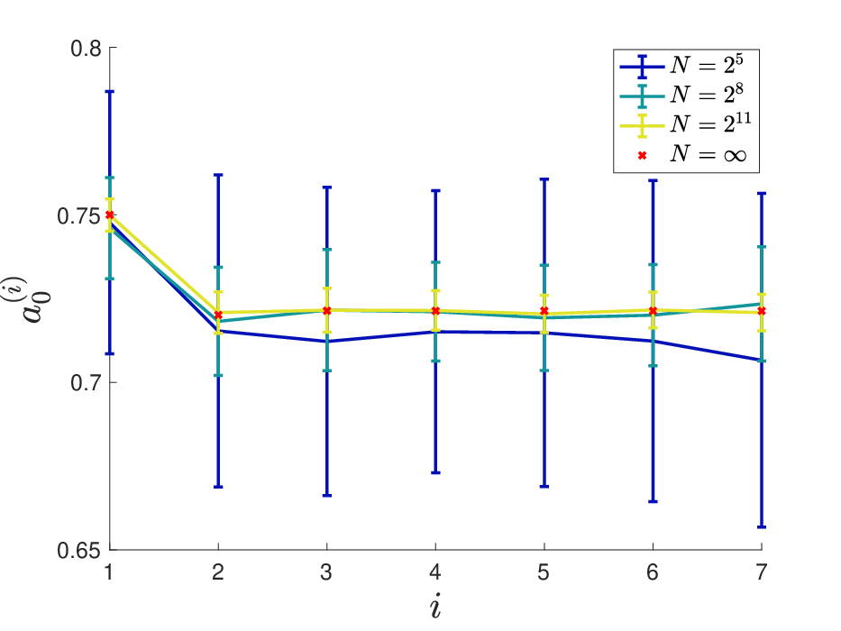
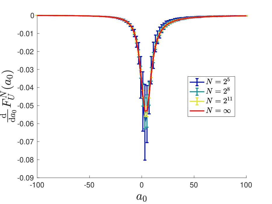
The limiting function corresponds to the idealized ADP algorithm with exact projections. We note that Assumption A6 holds since the above convergence rate is by the central limit theorem. In the left panel of Figure 8, we illustrate the distribution of the iterates with initialization for different number of particles. This plot shows how the estimates produced by the ADP algorithm concentrate around the fixed point iteration defined by .
We now turn our attention to Assumption A5. The derivative of with respect to is
where
denotes the derivative of (69) with respect to . As , we have
| (71) |
where
It is apparent from the right panel of Figure 8 that the idealized ADP algorithm with exact projection is a contraction. Moreover, for this particular example, the ADP algorithm is also a contraction (on average) even with a small number of particles.
Appendix E Connection to Kullback-Leibler control
The Kullback-Leibler (KL) divergence from to is defined as if the integral is finite and , and otherwise. The intent of this section is to show that defined in (19) is the optimal policy of an associated KL optimal control problem [57, 32]. Making this connection allows us to leverage existing methodology and analysis developed in the approximate dynamic programming literature [3, 58] in Sections 4.2 and 5.1 respectively.
Suppose that the current policy is and consider the following optimal control problem
| (72) |
where the set of admissible policies for the control problem is
and the cost functional can be written as
| (73) |
Using properties of KL divergence, it follows from Property 1 of Proposition 1 that defined in (19) solves the optimal control problem (72). Rewriting (73) gives
We shall henceforth redefine the cost functional (73) to remove the intractable constant that does not affect the minimizer of (72).
Given a policy , the corresponding value functions of the control problem are given by the expected cost-to-go from a fixed time and state (see for example [3, Section 2.1])
| (74) | ||||
In this notation, the total value of policy is given by
We now define the optimal value and optimal value functions w.r.t. by taking the infimum over the set
| (75) | ||||
and denote the minimizer (if it exists) as . We stress the dependence of both and on the current policy as it is omitted notationally. These minimization problems can be solved using a backward dynamic programming approach. From (74) and (75), we have the dynamic programming recursion
| (76) | ||||
The above is commonly referred to as the discrete time Bellman recursion.
Owing to the use of KL costs, the minimizations in (76) are tractable: assuming that the current policy satisfies , applying [14, Proposition 2.3] gives
| (77) | ||||
with infimum attained at for . Observe that the optimal value functions are simply logarithmic transformations of the optimal policy, and the dynamic programming recursion (77) corresponds to (19) in logarithmic scale. The optimal value is as we have adjusted the cost functional (73). Lastly, the finite KL condition guarantees existence of a unique minimizer that lies in . It should be clear from Proposition 1 that working with the subset is not necessary, i.e. such a condition is only required when we formulate as the optimal policy of a Kullback-Leibler control problem.
Appendix F A non-linear multimodal state space model
We consider a popular toy non-linear state space model [25, 34] which corresponds to working on and having
| (78) | ||||
for , where . We will employ the BPF as uncontrolled SMC, i.e. set and for . As the smoothing distribution (5) is highly multimodal, owing to the uncertainty of the sign of the latent process, this example is commonly used as a benchmark to assess the performance of SMC methods. Moreover, we observe from Figure 9 that this problem also induces complex multimodal optimal policies.
F.1 Approximate dynamic programming
To approximate these policies, we rely on the following flexible function classes
for all , which corresponds to a radial basis function (RBF) approximation of the optimal policy in the natural scale. With this choice of function classes, the approximate projections (31) can be implemented using non-linear least squares.
Given the output of a twisted SMC method based on the current policy, we adopt the following approach which is computationally more efficient. Firstly, we fix as a pre-specified bandwidth factor multiplied by the sample standard deviation of particles at time . Instead of performing the above logarithmic projections to learn the associated value functions, we fit the RBF approximation directly at the natural scale with for , as this can be efficiently implemented [37, p. 161] as a linear least squares problem with non-negativity constraints in . We note that care has to be taken to ensure that these computations are numerically stable. We then sort the estimated weights and keep as knots particles with the largest weights, as this avoids having to retain components with low weights. This selection procedure allows us to adaptively focus our computational effort on approximating the optimal policy at appropriate regions of the state space.
Writing as the weights, as the bandwidth and as the knots estimated by cSMC at iteration for , the policy at iteration has the form
| (79) |
where is a multi-index, , and
It follows that under policy (79), the initial distribution is a mixture of Gaussian distributions, Markov transition kernels are given by mixtures of Gaussian transition kernels and evaluation of the twisted potentials defined in (13) is tractable; exact expressions are given in Section I.1 of the Supplementary Material. Figure 9 shows that such a parameterization is flexible enough to provide an adequate approximation of the optimal policy.


F.2 Comparison of algorithmic performance
We investigate the use of cSMC when the observation noise is small, i.e. high signal-to-noise ratio, since this is the regime where BPF exhibits poor performance. To do so, we fix and simulate three sets of observations of length according to (78) as takes values in . We use particles in cSMC and iteration as preliminary runs indicate that policy refinement under the parameterization (79) provides little improvement, especially when additional computing time is taken into account. The number of particles in BPF is then chosen to match computational time. The number of components and bandwidth factor were tuned using preliminary runs. These algorithmic settings and the results obtained in independent repetitions of each method are summarized in Table 2. As expected, although the performance gains over BPF diminish as the observation noise increases, it can be substantial when is small.
| Observation noise | |||||
| Algorithm | BPF | ||||
| cSMC | |||||
Appendix G Linear quadratic Gaussian control
This section considers a Gaussian static model (Section 2.4) which will allow us to draw connections to concepts from the linear quadratic Gaussian (LQG) control literature [1]. Consider on and for some and symmetric positive definite . By conjugacy, the models (6) are Gaussian and for we have with
and
G.1 Riccati equation
We now show that the backward recursion (19) with initialized as a policy of constant one functions can be performed exactly to obtain analytic expressions of the optimal policy w.r.t. . First note that under the choice of forward and backward Markov transition kernels specified in Section 7 with pre-conditioner , the potentials (7) have the form
| (80) |
where
| (81) | ||||
for . For sufficiently small step size, observe that dropping terms in (81) gives which, as expected, recovers the AIS potentials (8). For notational convenience, we set as the zero matrix or vector of the appropriate size and write the mean of the Euler-Maruyama move as with and .
Proposition 6.
The optimal policy w.r.t. is given by
| (82) | ||||
where the coefficients are determined by the backward recursion
| (83) | ||||
for , with and initialization at .
Proof.
The backward recursion (83) for the coefficients is analogous to the Riccati equation in the context of LQG control. To illustrate the behaviour of these coefficients, we set the prior as , and the likelihood as for some and for and some (here denotes the Kronecker delta). The time evolution of these coefficients is plotted in the top row of Figure 10 for the problem setting , , . Noting that the optimal value of the Kullback-Leibler control problem (75) is
with , the dominant contribution that the constant has to suggests that it is important to estimate the constants in (82) to learn good policies. Moving from the bottom left to top left plot, observe that increasing the location parameter from to increases the magnitude of but leaves unchanged. This behaviour is evident from the expressions of and is unsuprising for as the parameter does not alter the ‘structure’ of the problem. The increase in the magnitude of shows that the optimally controlled SMC method achieves the desired terminal distribution by initializing
| (84) |
closer to the posterior distribution and taking larger drifts in
| (85) |
Comparing the plots in the bottom row reveals that the off-diagonal elements of vanish under independence. Therefore these terms should be taken into account for posterior distributions that are very correlated. Having obtained the optimal policy w.r.t. in a backward sweep, we may then simulate the optimally controlled SMC method in a forward pass. In Figure 11, we contrast the output of the uncontrolled SMC method with that of the optimally controlled.


G.2 Approximate dynamic programming
The ability to compute the optimal policy in this setting allows us to evaluate the effectiveness of ADP algorithm (31) under correct parameterization, i.e. select the function classes
This choice corresponds to function classes of the form (38), hence we can use linear least squares to estimate the coefficients at each iteration of cSMC – see (49) and (50). If denote the coefficients estimated at iteration of Algorithm 3 in step 2(b), it follows that the policy at iteration is given by
for where . Observe from (84) and (85) that we need to impose the following positive definite constraints
which can be done by projecting onto the set of real symmetric positive definite matrices [29]. In our numerical implementation, we find that these constraints are already satisfied when the step size is sufficiently small. Although the computational complexity of this ADP procedure is , it scales quite costly in dimension as computation of least squares estimators require inversion of matrices where . For problems with large , it might be worth considering the use of iterative linear solvers which offer reduced complexity. We note that it is possible to avoid learning the dependency in the policy and hence reduce computational complexity drastically; we do not exploit this observation here for simplicity of presentation but will do so for other applications.
Figure 12 displays the coefficients estimated by cSMC with iterations. It is striking that with particles, we are able to accurately estimate, in a single ADP iteration, the true coefficients in dimension (here ). That said, we typically need to increase with to prevent the Gram matrices (49) from being ill-conditioned. Moreover, we find that it is unnecessary to perform policy refinement in this example, as the estimated policies converge immediately to an invariant distribution that is very concentrated around the optimal policy (82), which is the fixed point of the idealized algorithm in Theorem 2 under correct parameterization. The performance of the resulting controlled SMC method is indistinguishable from that in Figure 11.


Appendix H Bayesian logistic regression
Consider a binary regression problem: each observation is modelled as an independent Bernoulli random variable with probability of success , where for is the logistic link function, denotes the unknown regression coefficients and the row of a model matrix . Hence the likelihood function and its gradient is given by
and
where is a given dataset of interest. Following [28], we specify a Gaussian prior distribution on of the form and .
H.1 Approximate dynamic programming
In view of Proposition 4 and the previous section on LQG control, we consider the function classes in (45). As before, coefficients at each iteration can be estimated by linear least squares and the policy at iteration has the form
for , where for . Assuming that the constraints , , are satisfied or imposed, then sampling from
and
| (86) |
with for is feasible and evaluation of the twisted potentials defined in (13) is tractable since
and
for . We note that imposing and letting depend on the argument in (45) is related to the approach in [33, 51], as (86) then corresponds to an Euler-Maruyama discretization of a controlled diffusion with an additive control . For this application, we set the pre-conditioner as and we illustrate in Figure 13 that the parameterization (45) provides a good approximation of the optimal policy on a particular dataset concerning modeling of heart diseases.


H.2 Comparison of algorithmic performance
We now perform a comparison of algorithms on the analysis of three real datasets77 7 Datasets were downloaded from the UCI machine learning repository and standardized before analysis. with different characteristics, in the same manner as Section 7.2. We use number of particles in cSMC and select the number of iterations using preliminary runs – see Figure 13. The number of particles used in AIS is then chosen to match computational cost, measured in terms of run time. These algorithmic settings and the results obtained using independent repetitions each of method are summarized in Table 3. Although AIS provides state-of-the-art results in complex scenarios for these models [12], the comparison shows that for all datasets considered, cSMC outperforms it and particularly so for the task of marginal likelihood estimation by several orders of magnitude.
| Dataset | |||||
| Heart disease | Australian credit | German credit | |||
| Algorithm | AIS | ||||
| cSMC | |||||
Appendix I Model specific expressions
I.1 Expressions for non-linear multimodal state space model
I.2 Expressions for Lorenz-96 model
I.3 Expressions for neuroscience model
Assume that the constraints , , are satisfied or imposed. Then the initial distribution
and the Markov transition kernels
for Moreover, the twisted potentials defined in (13) can be evaluated since
and
for .