Unification of Constant-roll Inflation and Dark Energy with Logarithmic -corrected and Exponential Gravity
Abstract
In this paper we investigate how to describe in a unified way a constant-roll inflationary era with a dark energy era, by using the theoretical framework of gravity. To this end, we introduce some classes of appropriately chosen gravity models, and we examine in detail how the unification of early and late-time acceleration eras can be achieved. We study in detail the inflationary era, and as we demonstrate it is possible to achieve a viable inflationary era, for which the spectral index of primordial curvature perturbations and the scalar-to-tensor ratio can be compatible with the latest observational data. In addition, the graceful exit issue is briefly discussed for a class of models. Finally, we discuss the dark energy oscillations issue, and we investigate which model from one of the classes we introduced, can produce oscillations with the smallest amplitude.
pacs
04.50.Kd, 04.60.Bc, 95.36.+x, 98.80.CqI Introduction
Modified gravity in it’s various forms, has a prominent role in describing the Universe’s evolution [1, 2, 3, 4, 5]. Particularly, a vast number of phenomena related to various stages of the Universe’s evolution can be explained by modified gravity theories, both at an astrophysical level and also at a galactic level, see for example the review [1]. Among the various theories of modified gravity, gravity is the most commonly used and, to our opinion, the most appealing modified gravity theory, due to the simplicity offered by gravity descriptions, but also due to the conceptual rigidity offered by this theory. Among other applications, the gravity theoretical framework, offers the possibility of a unified description of the early-time and late-time acceleration eras [6], see also Refs. [7] (for reviews on the unification of the early and late-time acceleration, see [1, 2, 3]). This unified description is one of the most demanding aims of a theoretical description, and various approaches towards this issue have been presented in the literature.
In the present work we aim to present some gravity models which can describe in a unified way a constant-roll inflationary era with a late-time acceleration era. The constant-roll inflation description, is an alternative approach to the standard slow-roll inflationary era, and it’s implications have recently been studied in the context of scalar-tensor theories [8, 9, 10, 11, 12, 13, 14, 15, Motohashi:2017aob, 16, 17, 18, 19, 20, 21], see also [22, 23, 24, 25] and also in the context of gravity [26, 27, 28]. As it was shown in [26], it is possible that non-viable gravity models in the context of slow-roll inflation, may become viable in the context of constant-roll inflation. As we will demonstrate, in the context of the constant-roll evolution, it is possible to obtain observational indices that are compatible with the Planck constraints. We shall use two well-known gravity models, namely an -corrected logarithmic model and a curvature corrected exponential model, and we explicitly calculate the spectral index of primordial curvature perturbations and the scalar-to-tensor ratio, and as we show, these are compatible with the observational data. Also we shall briefly discuss some interesting features of the reheating era corresponding to the -corrected logarithmic model. In addition, we analyze the late-time evolution corresponding to both the aforementioned gravity models, and it is noteworthy that these models provide a unified description of the late and early-time acceleration era. Finally, we analyze the dark energy oscillations for the curvature-corrected exponential model, and we demonstrate that the most phenomenologically appealing case corresponds to nearly curvature corrections.
This paper is organized as follows: In section II we introduce and study two models of gravity, and we investigate the constant-roll inflation implications on the inflationary era. For the -corrected logarithmic model of gravity we also briefly discuss the reheating era implications. In section III, we study the late-time evolution implications of the two models we introduced in the previous section, and for the curvature corrected exponential model, we investigate which curvature correction produces less dark energy oscillations during the last stages of the matter domination era and after the deceleration acceleration transition. Finally, the conclusions follow in the end of the paper.
Before we start, let us briefly present the conventions we shall assume. With regard to the geometric background, we assume that it is a flat Friedmann-Robertson-Walker (FRW), with the line element being,
| (I.1) |
where is the scale factor. In addition, we assume that the metric connection is an affine, torsion-less, and metric-compatible connection, the Levi-Civita connection. Also in the following, the parameter stands for , where is the Planck mass scale.
II The Inflationary Era with -corrected Logarithmic and Exponential Gravity
II.1 Model I of Inflation: -corrected Logarithmic gravity
The first model we shall consider has the following action,
| (II.2) |
where denotes the spacetime manifold, is the determinant of the metric tensor , is the Lagrangian of the matter and radiation perfect fluids and is the Ricci scalar. The corrections to the Hilbert-Einstein Lagrangian of General Relativity (GR) assume the form of -gravity and are represented by the higher curvature -term for the early-time inflation, and a function of the Ricci scalar, , for the dark energy sector. The running coefficient in front of depends also on the Ricci scalar and has been introduced in order for the graceful exit from inflation to be possible. When is constant, then the Starobinsky inflationary scenario is obtained, where the early-time de Sitter expansion is governed by an gravity.
The first Friedmann equation for the model at hand is the following,
| (II.3) | |||||
where the “dot” denotes the derivative with respect to the cosmic time and the “prime” denotes differentiation with respect to the Ricci scalar. The Ricci scalar reads,
| (II.4) |
with being the Hubble parameter. In the equation above, denotes the energy density of matter which satisfies the following conservation law,
| (II.5) |
where is the matter pressure.
In order to reproduce the early-time acceleration we introduce the following expression for the function ,
| (II.6) |
where is the curvature of the Universe at the end of inflation and are positive dimensional constants. Note that logarithmic corrections of the form appearing in Eq. (II.6) are actually motivated by one-loop corrections to coupling constants in multiplicatively renormalizable higher-derivative quantum gravity, for a general review, see [29]. Also it has been demonstrated [30, 31], that such an -corrected logarithmic gravity predicts viable inflation. Furthermore, these terms may also find a theoretical explanation in the framework of holographic renormalization group flow and the corresponding cosmological implications, in the context these issue were discussed in Refs. [32, 33]. In fact, if one incorporates in a gravitational system an holographic surface term, located near to the Hubble horizon, one obtains higher derivative corrections to the FRW field equations. Thus, the solutions of these equations may be used to describe the early-time acceleration and, eventually, by making use of two holographic screens, the late-time accelerated expansion of our Universe today may be realized.
Returning to the model at hand, it turns out that . Since we would like to avoid the effects of -gravity in the limit of small curvature, we require that the following general condition holds true,
| (II.7) |
where is the curvature of the Universe when the dark energy is dominant, and is the Cosmological constant. In the following, we will assume that and in (II.2) are negligible in the limit of high curvatures. The de Sitter solution with constant curvature follows from (II.3) and it reads,
| (II.8) |
In the case of a constant value of , namely for , the de Sitter solution is obtained as an asymptotic limit of the first Friedmann equation, when the -term is dominates the evolution. This is the so-called Starobinsky model, where the Hilbert-Einstein term guarantees a graceful exit from the accelerated phase. Since in the Starobinsky model , we have a regime of super-Planckian curvature. Here, the term has the same order of magnitude as the Hilbert-Einstein term during the inflationary era. In this case, the running constant in (II.6) with , determines the value of the de Sitter solution as in Eq. (II.8).
If we perturb the de Sitter solution as follows,
| (II.9) |
by keeping first order terms with respect to , we obtain from Eq. (II.3),
| (II.10) |
In the limit the solution of this equation reads,
| (II.11) |
where are constants depending on the sign of . When we choose the plus sign, the solution diverges and the de Sitter expansion is unstable. Thus, by Taylor expanding, the divergent solution is given by,
| (II.12) |
and in effect, we obtain,
| (II.13) |
where is the time at the end of inflation when and also , and stand for,
| (II.14) |
In order to study the behavior of the solution during the exit from inflation, we introduce the -foldings number,
| (II.15) |
By using Eq. (II.13) we have,
| (II.16) |
where we have assumed that , or equivalently . Thus, the Hubble parameter may be expressed as follows,
| (II.17) |
At the beginning of inflation we have and , while at the end of the early-time acceleration, when , one recovers .
During the quasi de Sitter expansion of inflation the Hubble parameter slowly decreases. The slow-roll parameters are defined as follows,
| (II.18) |
where we assumed that the constant-roll condition holds true. At the beginning of the early-time acceleration the first slow-roll parameter is small, in which case the slow-roll approximation regime is realized. For the solution (II.17) in the limit , we get,
| (II.19) |
On the other hand, for the parameter we obtain a constant value, namely,
| (II.20) |
This means that the model at hand satisfies the condition for constant-roll inflation. This fact has an important consequence on the form of the spectral index of primordial curvature perturbations, which will be independent from the total number of the -foldings during inflation. The inflationary paradigm offers two important predictions about the inhomogeneities of our Universe at a galactic scale. Particularly, the perturbations around the FRW metric lead to a non-flat spectral index and also lead to a non-zero scalar-to-tensor ratio .
In the case of -gravity, the inflationary indices have the following form,
| (II.21) |
By calculating these, we obtain,
| (II.22) |
We can see that in the computation of the spectral index we can omit the contribution of which tends to vanish for (like in the Einstein frame case of the Starobinsky inflation). Since the constant-roll inflationary condition is assumed, it turns out that this index is in fact independent on the total -foldings number.
The latest Planck data [34] constrain the spectral index and the scalar-to-tensor ratio as follows,
| (II.23) |
As a consequence, we must require in order to obtain a viable inflationary scenario. This means that at the beginning of inflation we have , a condition which solves the problem of initial conditions of the Friedmann Universe model we study.
We can compare this result with the one corresponding to the ordinary Starobinsky model with . In this case, the Hilbert-Einstein term of (II.3) evaluated on the background solution (specifically, ) can be inserted in the perturbed Friedmann equation and we obtain instead of Eq. (II.10), the following equation,
| (II.24) |
where, as we have discussed above, we have to consider . This equation implies the following,
| (II.25) |
where is appropriately chosen to be the time instance at the beginning of inflation. Note that now we can eliminate the non-linear term of the solution, such that and the slow-roll parameter in (II.18) is approximately equal to zero. We also require that for , when inflation ends, the Hubble parameter vanishes, namely,
| (II.26) |
such that,
| (II.27) |
For the -foldings number (II.15) we get,
| (II.28) |
As a consequence, the resulting Hubble rate solution has the following form,
| (II.29) |
When , the -foldings number is given by , and it is easy to verify that .
The first slow-roll parameter for the Starobinsky inflation is equal to,
| (II.30) |
and the spectral index and the scalar-to-tensor ratio are equal to,
| (II.31) |
Therefore, we must require in order to have concordance with the Planck data and therefore we need to specify the boundary value of the Hubble parameter as follows . In the model at hand, the first slow-roll parameter appearing in Eq. (II.19) decreases in exponential way, a behavior which is different in comparison to Eq. (II.30). However, when we obtain the same spectral index with the Starobinsky inflation with , but we need to point out that in our model, the total amount of inflation measured by the -foldings at the beginning of inflation, can be larger than . This fact contributes to easily suppress the value of the scalar-to-tensor ratio in Eq. (II.22), as it is strongly encouraged by the BICEP2/Keck-Array data [35].
By imposing in Eq. (II.14) we obtain,
| (II.32) |
and the expansion curvature rate during inflation is defined in this way. The characteristic curvature at the time of inflation is , in which case one has and from Eq. (II.7) we must require . Finally, the relation between and is fixed by Eq. (II.8) and we obtain,
| (II.33) |
II.1.1 The Reheating Era
At the end of the inflationary era, the model enters in a reheating phase. We will still assume that the contribution of the term in Eq. (II.3) is negligible, while the perfect fluid matter content of the Universe (namely, the energy density term ) has been shifted away, during the severe inflationary accelerated expansion that the Universe experienced, and has to be thermalized by the reheating process. During this phase, we will assume that the radiation/matter fields are bosonic scalar fields, which are described by the Klein-Gordon Lagrangian. By assuming that and by taking the limit (II.7), Eq. (II.3) reads,
| (II.34) |
The reheating solution takes place in an oscillatory phase, when the following holds true,
| (II.35) |
Thus, if one completely neglects the right hand side term of Eq. (II.34), we have with . In detail, one has to match the solution (II.13) with the new one in the form , where is a function of the time such that and (slowly-damping approximation). The form of the reheating (oscillatory) solution is [36],
| (II.36) |
where is the time when the reheating starts. For , the solution is given by (II.13) and therefore, the transition to the reheating phase takes place when , namely,
| (II.37) |
where we have expanded (II.13) with respect to . Since , if we use (II.16) we get,
| (II.38) |
with being the total -foldings of inflation. By equating (II.13) with (II.36) and by imposing , we can specify the frequency of the reheating solution as follows,
| (II.39) |
where we have used Eq. (II.8) and we have introduced the constant-roll parameter of Eq. (II.20).
For large values of the Hubble parameter behaves as follows,
| (II.40) |
Since , we get a matter dominated cosmological evolution. By taking into account that , we obtain,
| (II.41) |
The Lagrangian of a scalar bosonic field with mass , which is non-minimally coupled with gravity, is given by,
| (II.42) |
where is a coupling constant. Thus, the field equation is derived as follows,
| (II.43) |
As a consequence, the Fourier modes of the field with momentum for a FRW spacetime, satisfy the following differential equation,
| (II.44) |
By introducing the conformal time and also by redefining we have,
| (II.45) |
As a result, the oscillations of the Ricci scalar change the effective mass term and the number of massive particles increases with time. We note that, even in the case of minimal coupling with gravity , the effective mass still depends on the Ricci scalar and the reheating mechanism takes place.
The energy density of radiation-ultra-relativistic matter is related to the temperature as follows,
| (II.46) |
where is some constant. Since the energy density is connected to the square average of the Ricci scalar [36], from Eq. (II.41) we have and therefore we obtain,
| (II.47) |
where we used (II.39).
In the Starobinsky inflationary scenario, the equation (II.34) with solution (II.36) is still valid, but during the reheating era we have,
| (II.48) |
or equivalently,
| (II.49) |
with being the total number of -foldings during the inflationary era. In this case, the frequency in (II.36) results to be,
| (II.50) |
Thus, if we compare the reheating temperature of our model with the reheating temperature corresponding to the Starobinsky inflation , we find,
| (II.51) |
Since the constant-roll parameter in (II.20) for is small, we see that the temperature of the Universe after inflation predicted by our model is smaller respect to the one of the standard -scenario. This result shows that a constant-roll inflationary era has important effects on the reheating phase, as was also pointed out in Ref. [28].
II.2 Model II of Inflation: Curvature-corrected Exponential gravity with Constant-roll Evolution
II.2.1 Constant-roll Evolution in Gravity
In most theories of inflation in the context of gravity, it is common to adopt the slow-roll approximation, in order to produce the right amount of inflation that may be compatible with the observational data. In this section we shall deviate from the standard slow-roll approach, and we shall assume that a constant-roll era occurs during the inflationary era. The constant-roll inflationary paradigm was firstly used in the context of scalar-tensor theories [8, 9, 10, 11, 12, 13, 14, 15, 16, 17, 18, 19, 20, 21], see also [22, 23, 24, 25] and was extended in the context of gravity in [26, 27, 28]. As it was shown in [26], the most natural generalization of the constant-roll condition in the Jordan frame is the following,
| (II.52) |
where is some real parameter, which can be either positive or negative. The condition (II.52) is the most natural generalization of the constant-roll condition used in scalar-tensor approaches, which is,
| (II.53) |
since the condition (II.53) is nothing else but the second slow-roll index , which in the most general case is equal to . We shall assume that the theory is described by a vacuum gravity and also that the background is a flat FRW metric. Upon variation of the gravitational gravity action with respect to the metric, we get the following equations of motion,
| (II.54) | ||||
| (II.55) |
where stands for and also the “dot” denotes differentiation with respect to . The dynamics of inflation in the context of gravity are governed by four inflationary indices, , , which are defined as follows [37, 38, 39, 40, 41, 42, 1],
| (II.56) |
with the function being equal to,
| (II.57) |
Also for the calculation of the scalar-to-tensor ratio , the quantity is needed, which is defined as follows,
| (II.58) |
The spectral index of primordial curvature perturbations , in the case that , is equal to [37, 38, 39],
| (II.59) |
with being equal to,
| (II.60) |
The above relation is quite general and holds true not only in the case that , but also when . With regard to the scalar-to-tensor ratio, in the context of vacuum gravity theories, it is defined as follows,
| (II.61) |
where the quantity is given in Eq. (II.58) above, and for the specific case of a vacuum gravity, the scalar-to-tensor ratio is equal to,
| (II.62) |
The constant-roll condition (II.52), affects the inflationary indices of inflation , appearing in Eq. (II.56), which can be written as follows [26],
| (II.63) |
where and stand for and respectively.
It is conceivable that the inflationary dynamics crucially depend on the functional form of the gravity. We shall study a curvature corrected exponential gravity, which as we show, perfectly describes the early-time acceleration era. Also as we show in a later section, the late-time acceleration era is also successfully described by this model.
II.2.2 Constant-roll Evolution with Curvature-corrected Exponential Gravity
The constant-roll condition utterly changes the viability of an gravity model, as it was shown in Ref. [26]. Particularly, it is possible that an gravity model is not compatible with the observational data, when this is studied in the context of the slow-roll condition, however if the constant-roll condition is assumed, the model may be compatible with the observations, for a large range of values of the free parameters of the model. In this section we shall present one model of this sort, which is a curvature-corrected exponential model, with the functional form of the gravity being [43, 44],
| (II.64) |
where , , eV, is an arbitrary parameter [43, 44, 56] and is a positive real parameter. This model has quite appealing inflationary dynamics in the context of constant-roll inflation, as we now evince. Consider the first equation of Eq. (II.54), which for the model (II.64) and by assuming that during the inflationary era, it can be approximated as follows,
| (II.65) | ||||
where we have set and for notational simplicity. It is conceivable that the dynamical evolution is not affected by the terms containing the exponentials, at least in the era where the approximation holds true. By using the constant-roll condition (II.52) and after some algebraic manipulations, Eq. (II.65) can be simplified as follows,
| (II.66) |
The differential equation (II.66) can be analytically solved, with the solution being,
| (II.67) |
with being an arbitrary integration constant which plays no role in the dynamics of inflation, as we shall show. Also it is notable that the parameter appearing in Eq. (II.65), does not appear in the final differential equation that governs the dynamical evolution. Having the Hubble rate at hand, it is easy to calculate the slow-roll indices , , so by substituting Eq. (II.67) in Eq. (II.63), we obtain,
| (II.68) |
and by using these, the parameter defined in Eq. (II.60), is equal to,
| (II.69) |
and therefore in this case, the spectral index of primordial curvature perturbations can be cast after some algebra in the following form,
| (II.70) |
Accordingly, by using Eq. (II.62), the scalar-to-tensor ratio is found to be,
| (II.71) |
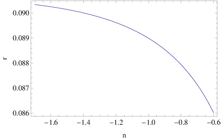
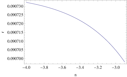
It is noteworthy that both the spectral index and the scalar-to-tensor ratio depend only on or . Having the final expressions for the spectral index and the scalar-to-tensor ratio at hand, we shall investigate the parameter space in order to see for which values of the free parameters, the compatibility with the observational data can be achieved. The latest Planck data [34] constrain the spectral index and the scalar-to-tensor ratio as in Eq. (II.23), so now we investigate which values of the parameters may render the curvature-corrected constant-roll model of Eq. (II.64) compatible with the Planck data. A detailed analysis reveals that there is a large range of parameter values that may render the model compatible with the observations. For example by choosing , the spectral index becomes and the corresponding scalar-to-tensor ratio becomes . Also for , the spectral index becomes and the corresponding scalar-to-tensor ratio becomes . Finally for , the spectral index becomes and the corresponding scalar-to-tensor ratio becomes . In Fig. 1 we plotted the functional dependence of the spectral index as a function of , for (left plot), and for (right plot). In both cases, In the red and black straight lines correspond to the Planck data allowed values for the spectral index, namely, and respectively.
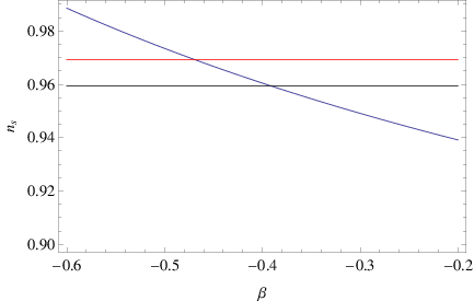
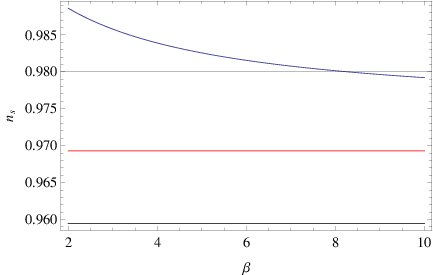
The same applies for the scalar-to-tensor ratio, and in Fig. 2, we plotted the functional dependence of the scalar-to-tensor ratio as a function of . In the left plot, the parameter is assumed to be , while in the right plot .
Concluding, we demonstrated that the curvature-corrected gravity model of Eq. (II.64) in the context of the constant-roll condition, provides an inflationary era which is compatible with the latest Planck data. An intriguing feature of the model (II.64), is that the parameter plays a crucial role in the late-time era. As we show in a later section, certain values of may produce an undesirable amount of dark energy oscillations, so the values of we used into this section, will be further constrained by the dark energy oscillations study.
Before we continue, it is worth discussing the resulting scalar-to-tensor ratio as it appears in Eq. (II.71). The resulting scalar-to-tensor ratio is quite an important result, that might be tested in the next generation of CMB experiments. So far, there have been several ground based CMB projects under design or already on going, which includes the CMB-S4 [46], BICEP3 [47], and AliCPT [48], and so on. It is interesting to note that, the operation of all these ground based experiments are able to cover the full CMB sky without the help of satellites such as WMAP or Planck, and correspondingly, the observational limit on the tensor-to-scalar ratio could be improved to about two orders of magnitude higher in comparison to the current one. This means that the parameter space of the models under consideration would be much constrained in the near future.
Before we close this section, it is worth discussing in brief the possibility of a graceful exit from the inflationary era, for the model (II.64). In general, the graceful exit issue can be a cumbersome task and also a conceptual challenge, especially in the context of gravity. In the literature, the graceful exit from inflation instance is identified with the time instance that the slow-roll approximation ceases to hold true, which occurs when the first slow-roll index becomes of the order . However, in Ref. [49] an alternative viewpoint was provided for the graceful exit from inflation issue. Particularly, the graceful exit from inflation could be triggered by the occurrence of growing curvature perturbations at some point during the inflationary era, which may disturb the inflationary attractor of the theory. In effect, the dynamical attractor becomes unstable, and hence ceases to be the final attractor of the theory, and the cosmological dynamical system is no longer described by this attractor, and therefore the dynamical cosmological evolution of inflation is interrupted. We believe that this way of thinking is conceptually more accurate for the description of the graceful exit from inflation.
So let us now investigate if the inflationary solution (II.67) ceases to be the final attractor of the cosmological system, and in order to see this, we linearly perturb this solution, as follows,
| (II.72) |
where we identify with the solution (II.67). By inserting Eq. (II.72) in the first equation of Eq. (II.54), and after some tedious algebraic manipulations, we obtain the following differential equation at leading order,
| (II.73) | ||||
which can be solved and the solution is,
| (II.74) |
A simple analysis can easily reveal the behavior of the perturbation , for the various values of the parameter , and in fact it can be shown that for , the perturbations decay as , while for , the perturbations grow as the time evolves to larger values. Thus, when , the cosmological solution of Eq. (II.67) is unstable towards linear perturbations, and therefore this can be viewed as a strong indication that the graceful exit from inflation actually happens in this case. However, the full study of this issue deserves an article focusing on this, since there are various questions that remain unanswered, for example, how many -foldings occur before the end of inflation, what happens when non-linear terms are taken into account and so on. Some of these tasks may prove quite difficult to address, since the lack of analyticity makes the problem quite cumbersome. We aim though in a future work, to address the aforementioned tasks by using an autonomous dynamical system approach.
III Late-time Acceleration Era
In this section we will investigate the behavior of the model I appearing in Eq. (II.2) during the late-time era. In order to do so, we need to introduce the dark energy part in the action, in terms of the function appearing in Eq. (II.2). We will use a modified version of exponential gravity, namely,
| (III.75) |
where is a positive parameter and is the cosmological constant. The function of the Ricci scalar is necessary to stabilize the theory at large redshifts and we shall assume that it has the following form,
| (III.76) |
where is a real and positive parameter. We need to note that, the existence of a quintom scenario where the equation of state (EoS) parameter evolves crossing the phantom divide line, is strictly connected with the possibility of having a stable de Sitter epoch at late times. This scenario is supported by cosmological observations, which allow an oscillatory behavior of the dark energy EoS parameter around the line of the phantom divide, although the data are still far from being conclusive. In this respect, an exhaustive review about the quintom scenario can be found in Ref. [50], where several successful examples of quintom cosmological models and their corresponding observational consequences were analyzed.
As a general feature of the model, we immediately see that, at , one has and we recover the Minkowski spacetime solution of Special Relativity. When , we obtain the standard evolution of the CDM model. Moreover, since , we have that the modification of gravity for the dark energy sector is completely negligible in the high curvature limit of the inflationary era, where .
We will now verify that with the modification we introduced in Eq. (III.75), it is possible to pass the cosmological and local tests. In order to do so, we introduce the following form of the gravity,
| (III.77) |
in which case the trace of the field equations results to the following equation,
| (III.78) |
where is the trace of the stress-energy tensor of the matter-radiation perfect fluids that quantify the matter content of the Universe. When , it is easy to see that the following conditions hold true,
| (III.79) |
The first condition is necessary in order to obtain the correct value of the Newton constant and avoid anti-gravitational effects during the matter, radiation and dark energy eras, while the second condition guarantees the stability of the model with respect to the matter perturbations [51, 52, 6].
When , which corresponds to the vacuum gravity case, the non-trivial solution of Eq. (III.78) is given by the de Sitter spacetime with . This is a consequence of the fact that and when . The perturbations around the de Sitter solution are governed by the equation,
| (III.80) |
For our model, the effective mass turns out to be positive, rendering the solution stable. This means that the de Sitter spacetime is a final attractor of the cosmological system for large values of the cosmic time, when in the expanding Universe the contents of matter and radiation vanish.
During the matter and radiation domination eras, the model we used mimics an effective cosmological constant, if the function in Eq. (III.76) is close to unity, namely
| (III.81) |
where recall that is the curvature of the Universe at the end of the inflationary era. For example, if , we obtain up to the value . For larger values of the curvature, matter and radiation dominate strongly the evolution. Moreover, the conditions (III.79) read,
| (III.82) |
The second condition always holds true for positive values of , but on the other hand, the first condition requires a careful investigation in order to avoid anti-gravitational effects in the large curvature limit. For example, assume that , then if , we obtain and it is obvious that this condition is satisfied.
III.1 The Radiation, Matter Domination Eras and Transition to Late-time Acceleration Era
In order to investigate the behavior of our model during radiation and matter domination eras, but also during the transition to the late-time era, and until present-time, we need to introduce the following variable,
| (III.83) |
which is known as the “scaled dark energy” [53, 1]. This variable encompasses the ratio between the effective dark energy and the standard matter density, evaluated at the present time, with the matter density defined as follows,
| (III.84) |
where is the mass scale associated with the Planck mass. In the expression (III.83), the variable denotes the redshift as usual, and also stands for .
If one extends the expression appearing in Eq. (III.77) as follows,
| (III.85) |
in order to include the entire form of the gravitational Lagrangian (II.2), it is possible to derive from the FRW field equations the following equation [53, 1],
| (III.86) |
where the functions , stand for,
| (III.87) | |||||
The Ricci scalar is easily derived from Eq. (III.83) and it is equal to,
| (III.88) |
At the late time regime, where , we can avoid the contribution of the matter and radiation fluids, in which case, the solution of Eq. (III.86) reads,
| (III.89) |
with being an integration constant. Since for the exponential gravity , the argument of the square root is positive, in effect, dark energy oscillates around the phantom divide line . The frequency of the oscillation with respect to is given by,
| (III.90) |
Generally speaking, since , the oscillation frequency at late times does not diverge. Such a problem may emerge in the high curvature regime, that is for redshifts that satisfy , when the contribution of the dark energy in Eq. (III.88) is negligible. In this case, after the expanding Eqs. (III.86)–(III.87) with respect to , we find the following solution in the vicinity of a given redshift [43, 44],
| (III.91) |
where is an integration constant. Here, the oscillation frequency of the dark energy is equal to,
| (III.92) |
As a consequence, when is very close to zero, like in the case of pure (vacuum) exponential gravity, the effective dark energy induced by modified gravity oscillates with high frequency and diverges, rendering the theory unstable. However in our model, due to the presence of the function chosen as in Eq. (III.76), one has,
| (III.93) |
This means that, back into the past, during the radiation and matter domination eras, the frequency of the effective dark energy oscillations, tend to decrease and the theory is protected against singularities.
III.2 Dark Energy Era for the Curvature-corrected Exponential Model
In this section we shall analyze certain features of the late-time evolution corresponding to the curvature-corrected exponential gravity model of Eq. (II.64), having to do with dark energy oscillations. It is known that certain viable models of dark energy produce dark energy density oscillations during the matter domination era, and the frequencies of these oscillations may diverge [43, 44, 54, 55]. In the modified gravity theories and especially in the gravity theories, fourth order derivatives appear in the theory, and hence high-frequency oscillations occur and the background may oscillate in a rapid way. In effect, perturbation theory may break down, since non-linearities may occur. It is therefore vital for gravity theories to overcome this theoretical obstacle. In this section we shall discuss this problem and by using some numerical analysis for the curvature corrected exponential model, and we shall investigate in which cases the dark energy oscillations may occur.
A convenient quantity that can easily quantify the dark energy oscillations is the scaled dark energy appearing in Eq. (III.86). Actually, by solving the differential equation (III.86) numerically we will be able to find how the dark energy oscillations behave at late-times, so for small redshifts. For our numerical analysis we shall use the following initial conditions [43, 44, 54, 55, 56],
| (III.94) |
with being and also is equal to eV2. In Fig. 3 we have plotted the scaled dark energy for three different values of the parameter , namely (blue curve), (red curve) and (black curve).
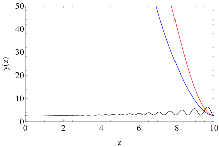
As we can see in Fig. 3, the scaled dark energy for the cases and behaves in a very similar way. Having the scaled dark energy at hand, we can easily investigate how the dark energy oscillations behave by studying the dark energy equation of state parameter , which in terms of is defined as follows,
| (III.95) |
In Fig. 4 we present the behavior of the dark energy equation of state parameter for (blue curve), (red curve) and (black curve).
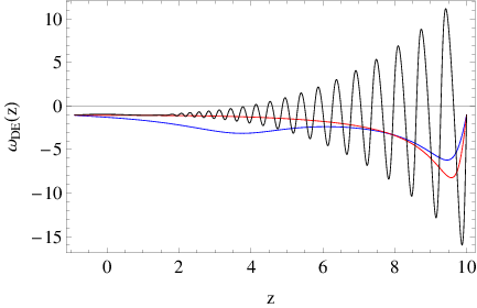
As it can be seen in Fig. 4, the oscillations have smaller amplitudes for , and these start during the matter domination era. In all cases, the dark energy oscillations stop to occur at small redshifts. It is noteworthy that the values of around , always provide the smaller amplitudes for the oscillations.
In order to have a clear picture for the physical behavior of the cosmological system, we shall investigate the behavior of the total equation of state parameter , as a function of the redshift , which in terms of is defined as follows,
| (III.96) |
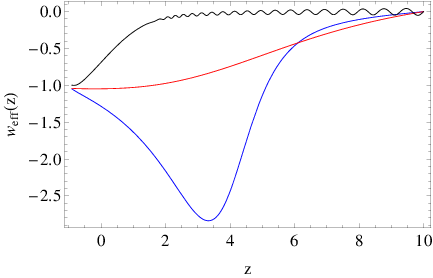
In Fig. (5) we plot the behavior of the total equation of state parameter as a function of the redshift , for (blue curve), (red curve) and (black curve). As it can be seen, the case has the mildest oscillatory behavior. It is noteworthy that in all cases, for small redshifts the phantom divide line is not crossed.
Finally, in Fig. 6 we plot the Hubble rate as a function of the redshift for (blue curve), (red curve) and (black curve). Note that in terms of the scaled dark energy parameter , the Hubble rate is defined as follows,
| (III.97) |
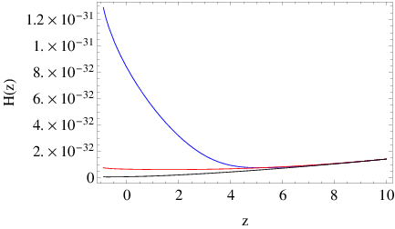
The analysis of the dark energy equation of state parameter and also of the total equation of state parameter, indicates strongly that the exponential model with nearly curvature corrections, has quite appealing properties, since the dark energy oscillations are less pronounced.
III.3 Dark Energy Oscillations for the Model I
Now let us investigate the dark energy oscillations issue for the model I appearing in Eqs. (II.2) and (II.6). We assume the following choices-conventions for the parameters,
| (III.98) |
where,
| (III.99) |
The second condition in Eq. (III.98) leads to a realistic de Sitter curvature for the early-time acceleration, which is . Moreover, the third condition in Eq. (III.98) ensures that the high curvature corrections of the model I disappear after the inflation, when .
The constant parameters of the function in Eqs. (III.75)–(III.76) are chosen as follows,
| (III.100) |
In this way, we obtain an optimal reproduction of the CDM model, and the effects of dark energy remain negligible during the early and mid stages of the matter and radiation eras.
Now we need to fix the boundary conditions of our cosmological dynamical system at large redshift . They can be inferred from the form of in Eq. (III.83) for the case of -modified gravity, namely,
| (III.101) |
When we obtain,
| (III.102) |
where and are functions of the redshift. At large redshift, during the matter era, we have to take and and the boundary conditions of the system are given by,
| (III.103) |
where,
| (III.104) |
For , in which case , and we effectively are in a matter dominated Universe, we obtain,
| (III.105) |
These values can be compared with the corresponding ones for the CDM model, where is a constant, namely . We argue that our model is extremely close to the CDM model at very high redshift. Here we recall that the first observed galaxies correspond to a redshift .
Finally, the contributions of matter and radiation are determined by the values of and in (III.83). The cosmological data indicate that,
| (III.106) |
By solving numerically the differential equation for in the redshift range, we obtained the results which appear in Fig. (7) and Fig. (8), where we plotted the behavior of and as a function of the redshift, for .
Despite of the fact that at high redshifts, the amplitude of the oscillations of the effective EoS parameter around the phantom divide line gradually grows, we see that their frequency decreases and thus, singularities are avoided.


In order to measure the matter energy density at a given redshift, we introduce the parameter as
| (III.107) |
In Fig. (9) the plot of is compared with the graphic of for . We see that is nearly constant and it is dominant over , for , a feature that is in full agreement with the CDM description.

The parameter,
| (III.108) |
is frequently used to express the ratio between the dark energy density and the effective energy density of our FRW Universe. Thus, by extrapolating at the current redshift , from Eqs. (III.108), we obtain,
| (III.109) |
The latest cosmological data [34] indicate that, and . Thus, our model fits the observational data at present time.
Hence, we have shown that the model I can mimic the late-time features of the CDM Model. The additional degree of freedom introduced by the -gravity, leads to an oscillatory behavior during the last stages of the matter domination era and the early stages of the dark energy era. However, the theory is stable and protected against singularities. We need to stress that in the simulation presented in this section, we have considered the whole form of the gravitational Lagrangian in (II.2). Thus, we confirm that the higher curvature corrections for inflation are negligible in the limit of small curvatures.
Conclusions
In this paper we demonstrated that it is possible to have a unified description of a constant-roll inflationary era with the dark energy era, by using two gravity models. Particularly, we used a -corrected logarithmic gravity model and a curvature-corrected exponential gravity model. With regard to the inflationary era, we demonstrated that it is possible to obtain observational indices compatible with the latest Planck data, in the context of constant-roll inflation. Particularly, the constant-roll condition broadens the parameter space, and this feature makes it more easy to have compatibility with the observational constraints.
In addition, we studied the late-time evolution of the gravity models. A noticeable feature related with the exponential model is that the dark energy oscillations have quite small amplitude when the curvature corrections are nearly of the form.
It would be interesting to analyze the possibility of having a unified description of constant-roll inflation with a dark energy era, in the context of other modified gravities, like for example Gauss-Bonnet or gravities, where it is possible to unify inflation with dark energy, see Ref. [1] for a comprehensive review. This issue deserves a study which we defer in a future work.
With regard to the graceful exit from inflation issue, which we briefly addressed for one of the inflationary models we presented in this paper, it should be noted that it deserves a more focused analysis. With the approach we adopted in this work, we provided hints that the graceful exit may occur as a result of growing curvature perturbations, and with exit from inflation we mean that an inflationary attractor solution may become unstable as the time evolves. In a more focused work, one should in principle construct an autonomous system of differential equations, and prove numerically that the inflationary attractors are indeed unstable stationary points of the dynamical system. Work is in progress towards the aforementioned line of research.
Finally, when gravitational systems different from the Einstein gravity are considered, we can find new cosmological solutions with a large variety of new features. In this work, we have seen that a constant roll inflation can be obtained by introducing higher derivative corrections in the action, while a quintom scenario for the dark energy can be obtained at late times, in the context of -gravity. A modified theory of gravity may also allow for an alternative description with respect to the Big Bang theory as in the bounce scenario, where a cosmological contraction is followed by an expansion at a finite time. The idea that instead from an initial singularity the universe has emerged from a cosmological bounce has been largely analyzed in the literature (see for example Refs. [57, 58, 59, 60, 61, 62] or Ref. [63] for bounce cosmology description in the context of teleparallel gravity).
Acknowledgments
This work is supported by MINECO (Spain), project FIS2013-44881, FIS2016-76363-P and by CSIC I-LINK1019 Project (S.D.O) and by Ministry of Education and Science of Russia Project No. 3.1386.2017 (S.D.O and V.K.O).
References
- [1] S. Nojiri, S. D. Odintsov and V. K. Oikonomou, arXiv:1705.11098 [gr-qc].
- [2] S. Nojiri, S.D. Odintsov, Phys. Rept. 505, 59 (2011);
- [3] S. Nojiri, S.D. Odintsov, eConf C0602061, 06 (2006) [Int. J. Geom. Meth. Mod. Phys. 4, 115 (2007)].
- [4] S. Capozziello, M. De Laurentis, Phys. Rept. 509, 167 (2011);
- [5] R. Myrzakulov, L. Sebastiani and S. Zerbini, Int. J. Mod. Phys. D 22, 1330017 (2013) [arXiv:1302.4646 [gr-qc]].
- [6] S.Nojiri and S. D. Odintsov, Phys. Rev. D68, 123512 (2003) [hep-th/0307288].
- [7] G. Cognola, E. Elizalde, S. Nojiri, S. D. Odintsov, L. Sebastiani and S. Zerbini, Phys. Rev. D 77, 046009 (2008) [arXiv:0712.4017 [hep-th]]; E. Elizalde, S. Nojiri, S. D. Odintsov, L. Sebastiani and S. Zerbini, Phys. Rev. D 83, 086006 (2011) [arXiv:1012.2280 [hep-th]].
- [8] S. Inoue and J. Yokoyama, Phys. Lett. B 524 (2002) 15 doi:10.1016/S0370-2693(01)01369-7 [hep-ph/0104083].
- [9] N. C. Tsamis and R. P. Woodard, Phys. Rev. D 69 (2004) 084005 doi:10.1103/PhysRevD.69.084005 [astro-ph/0307463].
- [10] W. H. Kinney, Phys. Rev. D 72 (2005) 023515 doi:10.1103/PhysRevD.72.023515 [gr-qc/0503017].
- [11] K. Tzirakis and W. H. Kinney, Phys. Rev. D 75 (2007) 123510 doi:10.1103/PhysRevD.75.123510 [astro-ph/0701432].
- [12] M. H. Namjoo, H. Firouzjahi and M. Sasaki, Europhys. Lett. 101 (2013) 39001 doi:10.1209/0295-5075/101/39001 [arXiv:1210.3692 [astro-ph.CO]].
- [13] J. Martin, H. Motohashi and T. Suyama, Phys. Rev. D 87 (2013) no.2, 023514 doi:10.1103/PhysRevD.87.023514 [arXiv:1211.0083 [astro-ph.CO]].
- [14] H. Motohashi, A. A. Starobinsky and J. Yokoyama, JCAP 1509 (2015) no.09, 018 doi:10.1088/1475-7516/2015/09/018 [arXiv:1411.5021 [astro-ph.CO]].
- [15] Y. F. Cai, J. O. Gong, D. G. Wang and Z. Wang, JCAP 1610 (2016) no.10, 017 doi:10.1088/1475-7516/2016/10/017 [arXiv:1607.07872 [astro-ph.CO]].
- [16] S. Hirano, T. Kobayashi and S. Yokoyama, Phys. Rev. D 94 (2016) no.10, 103515 doi:10.1103/PhysRevD.94.103515 [arXiv:1604.00141 [astro-ph.CO]].
- [17] L. Anguelova, Nucl. Phys. B 911 (2016) 480 doi:10.1016/j.nuclphysb.2016.08.020 [arXiv:1512.08556 [hep-th]].
- [18] J. L. Cook and L. M. Krauss, JCAP 1603 (2016) no.03, 028 doi:10.1088/1475-7516/2016/03/028 [arXiv:1508.03647 [astro-ph.CO]].
- [19] K. S. Kumar, J. Marto, P. Vargas Moniz and S. Das, JCAP 1604 (2016) no.04, 005 doi:10.1088/1475-7516/2016/04/005 [arXiv:1506.05366 [gr-qc]].
- [20] S. D. Odintsov and V. K. Oikonomou, JCAP 1704 (2017) no.04, 041 doi:10.1088/1475-7516/2017/04/041 [arXiv:1703.02853 [gr-qc]].
- [21] S. D. Odintsov and V. K. Oikonomou, arXiv:1704.02931 [gr-qc].
- [22] J. Lin, Q. Gao and Y. Gong, Mon. Not. Roy. Astron. Soc. 459 (2016) no.4, 4029 doi:10.1093/mnras/stw915 [arXiv:1508.07145 [gr-qc]].
- [23] Q. Gao and Y. Gong, arXiv:1703.02220 [gr-qc].
- [24] Q. Gao, arXiv:1704.08559 [astro-ph.CO].
- [25] Q. Fei, Y. Gong, J. Lin and Z. Yi, arXiv:1705.02545 [gr-qc].
- [26] S. Nojiri, S. D. Odintsov and V. K. Oikonomou, arXiv:1704.05945 [gr-qc].
- [27] H. Motohashi and A. A. Starobinsky, arXiv:1704.08188 [astro-ph.CO].
- [28] V. K. Oikonomou, “Reheating in Constant-roll Gravity,” arXiv:1706.00507 [gr-qc].
- [29] I. L. Buchbinder, S. D. Odintsov and I. L. Shapiro, “Effective action in quantum gravity,” Bristol, UK: IOP (1992) 413 p
- [30] E. Elizalde, S. D. Odintsov, L. Sebastiani and R. Myrzakulov, Nucl. Phys. B 921 (2017) 411 doi:10.1016/j.nuclphysb.2017.06.003 [arXiv:1706.01879 [gr-qc]].
- [31] R. Myrzakulov, S. Odintsov and L. Sebastiani, Phys. Rev. D 91 (2015) no.8, 083529 doi:10.1103/PhysRevD.91.083529 [arXiv:1412.1073 [gr-qc]].
- [32] Y. F. Cai and E. N. Saridakis, Phys. Lett. B 697 (2011) 280 doi:10.1016/j.physletb.2011.02.020 [arXiv:1011.1245 [hep-th]].
- [33] Y. F. Cai, J. Liu and H. Li, Phys. Lett. B 690 (2010) 213 doi:10.1016/j.physletb.2010.05.033 [arXiv:1003.4526 [astro-ph.CO]].
- [34] P. A. R. Ade et al. [Planck Collaboration], arXiv:1502.01589 [astro-ph.CO].
- [35] P. A. R. Ade et al. [BICEP2 and Keck Array Collaborations], Phys. Rev. Lett. 116 (2016) 031302 doi:10.1103/PhysRevLett.116.031302 [arXiv:1510.09217 [astro-ph.CO]].
- [36]
A. Vilenkin,
Phys. Rev. D 32 (1985) 2511.
doi:10.1103/PhysRevD.32.2511;
M. B. Mijic, M. S. Morris and W. M. Suen, Phys. Rev. D 34 (1986) 2934. - [37] H. Noh and J. c. Hwang, Phys. Lett. B 515 (2001) 231 [astro-ph/0107069].
- [38] J. c. Hwang and H. r. Noh, Phys. Rev. D 65 (2002) 023512 doi:10.1103/PhysRevD.65.023512 [astro-ph/0102005].
- [39] J. c. Hwang and H. Noh, Phys. Lett. B 506 (2001) 13 doi:10.1016/S0370-2693(01)00404-X [astro-ph/0102423].
- [40] S. Nojiri, S. D. Odintsov and V. K. Oikonomou, Phys. Rev. D 94 (2016) no.10, 104050 doi:10.1103/PhysRevD.94.104050 [arXiv:1608.07806 [gr-qc]].
- [41] S. D. Odintsov and V. K. Oikonomou, Class. Quant. Grav. 33 (2016) no.12, 125029 doi:10.1088/0264-9381/33/12/125029 [arXiv:1602.03309 [gr-qc]].
- [42] S. D. Odintsov and V. K. Oikonomou, Phys. Rev. D 92 (2015) no.12, 124024 doi:10.1103/PhysRevD.92.124024 [arXiv:1510.04333 [gr-qc]].
- [43] E. Elizalde, S. D. Odintsov, L. Sebastiani and S. Zerbini, Eur. Phys. J. C 72 (2012) 1843 [arXiv:1108.6184 [gr-qc]].
- [44] K. Bamba, A. Lopez-Revelles, R. Myrzakulov, S. D. Odintsov and L. Sebastiani, Class. Quant. Grav. 30, 015008 (2013) [arXiv:1207.1009 [gr-qc]].
- [45] V. K. Oikonomou, N. Karagiannakis and M. Park, Phys. Rev. D 91 (2015) no.6, 064029 [arXiv:1411.3199 [gr-qc]].
- [46] K. N. Abazajian et al. [CMB-S4 Collaboration], arXiv:1610.02743 [astro-ph.CO].
- [47] H. Hui et al. [BICEP3 Collaboration], Proc. SPIE Int. Soc. Opt. Eng. 9914 (2016) 99140T doi:10.1117/12.2232986 [arXiv:1607.06861 [astro-ph.IM]].
- [48] Y. F. Cai and X. Zhang, Sci. China Phys. Mech. Astron. 59 (2016) no.7, 670431 doi:10.1007/s11433-016-0178-x [arXiv:1605.01840 [astro-ph.IM]].
- [49] K. Bamba, R. Myrzakulov, S. D. Odintsov and L. Sebastiani, Phys. Rev. D 90 (2014) no.4, 043505 doi:10.1103/PhysRevD.90.043505 [arXiv:1403.6649 [hep-th]].
- [50] Y. F. Cai, E. N. Saridakis, M. R. Setare and J. Q. Xia, Phys. Rept. 493 (2010) 1 doi:10.1016/j.physrep.2010.04.001 [arXiv:0909.2776 [hep-th]].
- [51] A. D. Dolgov and M. Kawasaki, Phys. Lett. B 573, 1 (2003) [astro-ph/0307285]; V. Faraoni, Phys. Rev. D 74, 104017 (2006) [arXiv:astro-ph/0610734].
- [52] Y. S. Song, W. Hu and I. Sawicki, Phys. Rev. D 75, 044004 (2007) [arXiv:astro-ph/0610532].
- [53] K. Bamba, C. Q. Geng and C. C. Lee, JCAP 1008, 021 (2010) [arXiv:1005.4574 [astro-ph.CO]]; C. Q. Geng, C. C. Lee and Shan Lin, arXiv:1506.03253v2 [astro-ph.CO]; Y. Chen, C. Q. Geng, C. C. Lee, L. W. Luo and Z. H. Zhu, Phys. Rev. D 91, no. 4, 044019 (2015) [arXiv:1407.4303 [astro-ph.CO]].
- [54] H. Motohashi, A. A. Starobinsky and J. ’i. Yokoyama, JCAP 1106, 006 (2011) [arXiv:1101.0744 [astro-ph.CO]].
- [55] J. Matsumoto, Phys. Rev. D 87, no. 10, 104002 (2013) [arXiv:1303.6828 [hep-th]].
- [56] V. K. Oikonomou, N. Karagiannakis and M. Park, Phys. Rev. D 91 (2015) no.6, 064029 [arXiv:1411.3199 [gr-qc]].
- [57] Y. F. Cai, T. Qiu, Y. S. Piao, M. Li and X. Zhang, JHEP 0710 (2007) 071 doi:10.1088/1126-6708/2007/10/071 [arXiv:0704.1090 [gr-qc]].
- [58] Y. F. Cai, S. H. Chen, J. B. Dent, S. Dutta and E. N. Saridakis, Class. Quant. Grav. 28 (2011) 215011 doi:10.1088/0264-9381/28/21/215011 [arXiv:1104.4349 [astro-ph.CO]].
- [59] Y. F. Cai, D. A. Easson and R. Brandenberger, JCAP 1208 (2012) 020 doi:10.1088/1475-7516/2012/08/020 [arXiv:1206.2382 [hep-th]].
- [60] S. D. Odintsov and V. K. Oikonomou, Phys. Rev. D 94 (2016) no.6, 064022 doi:10.1103/PhysRevD.94.064022 [arXiv:1606.03689 [gr-qc]].
- [61] S. D. Odintsov and V. K. Oikonomou, Int. J. Mod. Phys. D 26 (2017) no.08, 1750085 doi:10.1142/S0218271817500857 [arXiv:1512.04787 [gr-qc]].
- [62] J. Haro, A. N. Makarenko, A. N. Myagky, S. D. Odintsov and V. K. Oikonomou, Phys. Rev. D 92 (2015) no.12, 124026 doi:10.1103/PhysRevD.92.124026 [arXiv:1506.08273 [gr-qc]].
- [63] Y. F. Cai, S. Capozziello, M. De Laurentis and E. N. Saridakis, Rept. Prog. Phys. 79 (2016) no.10, 106901 doi:10.1088/0034-4885/79/10/106901 [arXiv:1511.07586 [gr-qc]].