跳到论文正文
W Papers独立论文阅读器 arXiv:1708.08345 论文正文 计算阅读时间 · 0%
引用这篇论文根据当前论文元数据生成,正式投稿前建议核对。


License: arXiv.org perpetual non-exclusive license
arXiv:1708.08345v1 [math.NA] 25 Aug 2017

Recovering an Unknown Source in a Fractional Diffusion Problem

William Rundell ††thanks: rundell@math.tamu.edu Affiliation: Department of Mathematics, Texas A&M University, USA    Zhidong Zhang ††thanks: zhidong.zhang@helsinki.fi Affiliation: Department of Mathematics and Statistics, University of Helsinki, Finland
Abstract

A standard inverse problem is to determine a source which is supported in an unknown domain DD from external boundary measurements. Here we consider the case of a time-dependent situation where the source is equal to unity in an unknown subdomain DD of a larger given domain Ω\Omega. Overposed measurements consist of time traces of the solution or its flux values on a set of discrete points on the boundary ∂Ω\partial\Omega. The case of a parabolic equation was considered in [5]. In our situation we extend this to cover the subdiffusion case based on an anomalous diffusion model and leading to a fractional order differential operator. We will show a uniqueness result and examine a reconstruction algorithm. One of the main motives for this work is to examine the dependence of the reconstructions on the parameter α\alpha, the exponent of the fractional operator which controls the degree of anomalous behavior of the process. Some previous inverse problems based on fractional diffusion models have shown considerable differences between classical Brownian diffusion and the anomalous case.

1 Introduction

Our aim is to recover the location and shape of an extended source function F=χ⁡(D)F=\chi(D) in a diffusion problem from making time-trace boundary measurements,

{DαtC​u−△​u=χD,(x,t)∈Ω×(0,T);u⁡(x,0)=0,x∈Ω;u⁡(x,t)=0,(x,t)∈∂Ω×(0,T).\begin{cases}\begin{aligned} {}^{C}\!D_{t}^{\alpha}u-\triangle u&=\chi_{{}_{D}},&&(x,t)\in\Omega\times(0,T);\\ u(x,0)&=0,&&x\in\Omega;\\ u(x,t)&=0,&&(x,t)\in\partial\Omega\times(0,T).\end{aligned}\end{cases} (1.1)

Ω⊆ℝ2\Omega\subseteq\mathbb{R}^{2} is the unit disc, χD\chi_{{}_{D}} is the characteristic function on DD which is the source domain we need to recover with D¯⊆Ω\overline{D}\subseteq\Omega. The overposed data is a time trace of the flux at a (small) finite number mm of points located on the boundary ∂D\partial D,

∂u∂𝐧→(zℓ,t)=gℓ(t),t∈[0,T],ℓ=1,…,m.\frac{\partial u}{\partial{\overrightarrow{\bf n}}}(z_{\ell},t)=g_{\ell}(t),\ t\in[0,T],\ \ell=1,\dots,m.

In this paper, we restrict the set of admissible boundaries to be star-like domains with respect to a point within Ω\Omega,

∂D={q⁡(θ)​(cos⁡θ,sin⁡θ)⊤:θ∈[0,2​π]}\partial D=\{q(\theta)(\cos{\theta},\sin{\theta})^{\top}:\theta\in[0,2\pi]\}

with a smooth, periodic function 0<q⁡(θ)<10<q(\theta)<1. In equation  (1.1) DαtC{}^{C}\!D_{t}^{\alpha} denotes the Djrbashian-Caputo fractional derivative of order α\alpha, 0<α<10<\alpha<1 which will be defined in the next section.

We have described (1.1) in the simplest setting in the sense we have taken the exterior boundary to be the unit circle and have chosen homogeneous initial and boundary data. This simplifies the exposition and, in particular, many of the representation formulae. Adding in nonhomogeneous initial/boundary conditions: u​(x,0)=u0​(x)u(x,0)=u_{0}(x) and u⁡(x,t)=f⁡(x,t)u(x,t)=f(x,t) for xx on ∂Ω\partial\Omega and sufficiently smooth ff, would be completely straightforward. We could also have assumed a source of the form a⁡(t)​χ​(D)a(t)\chi(D) where a⁡(t)∈L∞​(0,∞)a(t)\in L^{\infty}(0,\infty) is known. In each of these cases no technical issues would ensue or changes to the main results. Taking Ω\Omega to be a simply connected domain with C2C^{2} boundary ∂Ω\partial\Omega is also possible in theory but we have used the specific eigenfunction expansion for −△-\triangle for a circle in both the uniqueness result and the reconstruction algorithm. The key change would be to equations (3.4) and (3.9) where the trigonometric function would have to be replaced by the values of the Laplace eigenfunction for Ω\Omega evaluated on ∂Ω\partial\Omega. While these share the same properties when Ω\Omega is the unit circle, this extension would require some further analysis.

The model (1.1) represents a so-called anomalous diffusion process generalizing classical, Brownian diffusion based on the heat equation. This latter model can be viewed as a random walk in which the dynamics are governed by an uncorrelated, Markovian, Gaussian stochastic process. The key assumption is that a change in the direction of motion of a particle is random and that the mean-squared displacement over many changes is proportional to time, i.e. ⟨x2⟩=C​t\langle x^{2}\rangle=Ct. This easily leads to the derivation of the underlying differential equation being the heat equation. On the other hand, when the random walk involves correlations, non-Gaussian statistics or a non-Markovian process (for example, due to “memory” effects) the classical diffusion equation will fail to describe the macroscopic limit. For example, if we replace the space-time correlation by ⟨x2⟩=C​tα\langle x^{2}\rangle=Ct^{\alpha} then it can be shown that this leads to a subdiffusive process and, importantly leads to a tractable model where the partial differential equation is replaced by the nonlocal equation (1.1).

This paper is a generalisation of [5] where the same problem was considered for the classical parabolic case, α=1\alpha=1. Our approach will be the same, but here we must deal with the technical issues of replacing the far simpler classical time derivative by the nonlocal operator DtαaC{}_{a}^{C}\!D_{t}^{\alpha}. Thus while in the case α=1\alpha=1 (1.1) is pointwise defined and the Markovian property dictates that for any time step tt the solution can be uniquely obtained from any single previous step t−δ​tt-\delta t, this is far from the case if α<1\alpha<1 where the complete time history of the function uu has to be retained in the evolution. In some previous cases involving fractional derivatives the inverse problem has very different properties, especially with respect to degree of ill-conditioning, from the classical case, see [8] for an overview. The poster child here is the backward diffusion problem. This is severely ill-conditioned for the heat equation, but for 0<α<10<\alpha<1 is only moderately so (equal to a 2-derivative loss) , [2]. Thus an important aspect of our studies here is to determine, if any, the differences made by the anomalous diffusion operator from that of the classical one. We will also investigate the influence of the number mm of measurement points on both the question of uniqueness and reconstruction.

2 Preliminary material

2.1 Fractional derivatives

The (left-sided) fractional integral of order α\alpha is defined for f∈L1​(a,b)f\in L^{1}(a,b) by

(Iαxa​f)​(x)=1Γ⁡(α)​∫ax(x−s)α−1​f​(s)​𝑑s,({{}_{a}I_{x}^{\alpha}}f)(x)=\frac{1}{\Gamma(\alpha)}\int_{a}^{x}(x-s)^{\alpha-1}f(s)\,ds, (2.1)

and leads naturally to a fractional derivative in one of two ways. The (left-sided) Riemann-Liouville fractional derivative of order 0<α<10<\alpha<1, is defined by

DtαaR​f​(t):=1Γ⁡(1−α)​dd​t​∫at(t−s)−α​f​(s)​𝑑s,{}_{a}^{R}\!D_{t}^{\alpha}f(t):=\frac{1}{\Gamma(1-\alpha)}\frac{d\ }{dt}\int_{a}^{t}(t-s)^{-\alpha}f(s)\,ds,

and the (left-sided) Djrbashian-Caputo fractional derivative of order α\alpha by

DtαaC​f​(t):=1Γ⁡(1−α)​∫at(t−s)−α​f′​(s)​𝑑s.{}_{a}^{C}\!D_{t}^{\alpha}f(t):=\frac{1}{\Gamma(1-\alpha)}\int_{a}^{t}(t-s)^{-\alpha}f^{\prime}(s)\,ds.

In both cases note the specific dependence on the endpoint aa. Some references are [3, 4, 1, 11, 12].

The Djrbashian-Caputo derivative is more restrictive than the Riemann-Liouville since it requires the classical derivative to be absolutely integrable and we implicitly assume that this condition holds. Generally, the Riemann-Liouville and Djrbashian-Caputo derivatives are different, even when both derivatives are defined, and we only have to consider the constant function to see this. Nonetheless, as we must expect, they are closely related to each other and under the assumption that the function to which they are applied vanishes at the starting point they are equal. Thus in (1.1) as stated we could have equally replaced Dtα0C{}_{0}^{C}\!D_{t}^{\alpha} by Dtα0R{}_{0}^{R}\!D_{t}^{\alpha}. However, in the face of a non-homogeneous initial condition the regularity of the solution of the direct problem for (1.1) would change.

2.2 Mittag-Leffler function

This function plays a central role in fractional diffusion equations. It is a two-parameter function defined as

Eα,β​(z)=∑k=0∞zkΓ⁡(k​α+β),z∈ℂ.E_{\alpha,\beta}(z)=\sum_{k=0}^{\infty}\frac{z^{k}}{\Gamma(k\alpha+\beta)},\ z\in\mathbb{C}.

The Mittag-Leffler function generalizes the exponential function since E1,1​(z)=ezE_{1,1}(z)=e^{z} and as α→1\alpha\to 1 the fractional diffusion process recovers classical diffusion as described by the heat equation. The following property will be used later. The proof can be found in standard references, for example, [11, Lemma 3.23.2].

Lemma 2.1.

For λ>0,α>0\lambda>0,\ \alpha>0 and n∈ℕ+,n\in\mathbb{N}^{+}, we have

dnd​tn​Eα,1​(−λ​tα)=−λ​tα−n​Eα,α−n+1​(−λ​tα),t>0.\frac{d^{n}}{dt^{n}}E_{\alpha,1}(-\lambda t^{\alpha})=-\lambda t^{\alpha-n}E_{\alpha,\alpha-n+1}(-\lambda t^{\alpha}),\ t>0.

In particular, dd​t​Eα,1​(−λ​tα)=−λ​tα−1​Eα,α​(−λ​tα)\frac{d}{dt}E_{\alpha,1}(-\lambda t^{\alpha})=-\lambda t^{\alpha-1}E_{\alpha,\alpha}(-\lambda t^{\alpha}), t>0\;t>0.

2.3 The direct problem for equation (1.1)

For the unit disc Ω,\Omega, denote the eigensystem of the Laplacian −△-\triangle with the Dirichlet boundary condition by {(λn,φn​(x)):n∈ℕ+}.\{(\lambda_{n},\varphi_{n}(x)):n\in\mathbb{N}^{+}\}. Here, {λn:n∈ℕ+}\{\lambda_{n}:n\in\mathbb{N}^{+}\} is indexed by nondecreasing order and strictly positive, and {φn​(x):n∈ℕ+}\{\varphi_{n}(x):n\in\mathbb{N}^{+}\} constitutes an orthonormal basis in L2​(Ω).L^{2}(\Omega). The polar representation of φn\varphi_{n} is

φn​(r,θ)=wn​Jm​(λn​r)​cos⁡(m​θ+ϕn),\varphi_{n}(r,\theta)=w_{n}J_{m}(\sqrt{\lambda_{n}}r)\cos{(m\theta+\phi_{n})}, (2.2)

where m=m⁡(n)m=m(n), the phase ϕn\phi_{n} is either 00 or π/2\pi/2 and wnw_{n} is the normalized weight factor. Here Jm​(z)J_{m}(z) is the first kind Bessel function with degree mm.

With the above, [11] gives the following theorem for the direct problem of (1.1). Here Hk​(Ω)H^{k}(\Omega) are the usual Sobolev spaces.

Theorem 2.1.

There exists a unique weak solution u∈L2​(0,T,H2​(Ω)∩H01​(Ω))u\in L^{2}(0,T;H^{2}(\Omega)\cap H_{0}^{1}(\Omega)) of (1.1) with the representation

u⁡(x,t)=∑n=1∞(∫0t∫Dφn​(y)​(t−τ)α−1​Eα,α​(−λn​(t−τ)α)​𝑑y​𝑑τ)​φn​(x)u(x,t)=\sum_{n=1}^{\infty}\left(\int_{0}^{t}\int_{D}\varphi_{n}(y)(t-\tau)^{\alpha-1}E_{\alpha,\alpha}(-\lambda_{n}(t-\tau)^{\alpha})\ {\rm d}y\ {\rm d}\tau\right)\varphi_{n}(x) (2.3)

and the regularity estimate

∥u∥L2​(0,T,H2​(Ω))+∥CDtα∥L2​(Ω×(0,T))≤C(T,D),\|u\|_{L^{2}(0,T;H^{2}(\Omega))}+\|^{C}\!D_{t}^{\alpha}\|_{L^{2}(\Omega\times(0,T))}\leq C(T,D),

where the notation C⁡(T,D)C(T,D) indicates the dependence on the final time TT and the domain DD.

Proof.

This theorem is a specific case of [11, Theorem 2.2] based on the fact that the source term is independent of tt. See a later remark about generalizing the situation in (1.1) to include a known time-dependent factor in the source term. ∎

3 Main results

In this section we will prove the main theoretical result: under suitable restrictions, two observation points are sufficient to determine the internal domain DD uniquely.

3.1 Harmonic basis

Let ξmc,s(r,θ)=1πrm{cosmθ,sinmθ:m∈ℕ}\xi_{m}^{c,s}(r,\theta)=\frac{1}{\pi}r^{m}\{\cos{m\theta},\sin{m\theta}:m\in\mathbb{N}\} denote the set of harmonic functions in Ω\Omega. With the given normalization it forms a complete orthonormal basis in L2​(∂Ω)L^{2}(\partial\Omega). First, we show that this basis can be used to gain a convergent approximation to the flux data ∂u∂𝐧→​(zℓ,t).\frac{\partial u}{\partial{\overrightarrow{\bf n}}}(z_{\ell},t).

Define the smooth approximation ψℓM∈C∞​(Ω¯)\psi_{\ell}^{M}\in C^{\infty}(\overline{\Omega}) of the delta distribution at zℓz_{\ell} as

ψℓM(x)=∑m=1Mξmc(zℓ)ξmc(x)+ξms(zℓ)ξms(x),ℓ=1,2,\psi_{\ell}^{M}(x)=\sum_{m=1}^{M}\xi_{m}^{c}(z_{\ell})\xi_{m}^{c}(x)+\xi_{m}^{s}(z_{\ell})\xi_{m}^{s}(x),\ \ell=1,2,

then the set uℓMu_{\ell}^{M} are weak solutions of the FDEs

{DαtC​uℓM−△​uℓM=0,(x,t)∈Ω×(0,T);uℓM=0,(x,t)∈∂Ω×(0,T);uℓM=−ψℓM,(x,t)∈Ω×{0}.\begin{cases}\begin{aligned} {}^{C}\!D_{t}^{\alpha}u_{\ell}^{M}-\triangle u_{\ell}^{M}&=0,&&(x,t)\in\Omega\times(0,T);\\ u_{\ell}^{M}&=0,&&(x,t)\in\partial\Omega\times(0,T);\\ u_{\ell}^{M}&=-\psi_{\ell}^{M},&&(x,t)\in\Omega\times\{0\}.\end{aligned}\end{cases}

It follows from [11] that we have the regularity results uℓM∈C⁡((0,T],H2​(Ω)∩H01​(Ω))u_{\ell}^{M}\in C((0,T];H^{2}(\Omega)\cap H_{0}^{1}(\Omega)), DαtC​uℓM∈C⁡((0,T],L2​(Ω)){}^{C}\!D_{t}^{\alpha}u_{\ell}^{M}\in C((0,T];L^{2}(\Omega)).

Lemma 3.1.

Define wℓM=uℓM+ψℓM,w_{\ell}^{M}=u_{\ell}^{M}+\psi_{\ell}^{M}, then wℓM∈C⁡((0,T],H2​(Ω)∩H01​(Ω)),w_{\ell}^{M}\in C((0,T];H^{2}(\Omega)\cap H_{0}^{1}(\Omega)), DαtC​wℓM∈C⁡((0,T],L2​(Ω)){}^{C}\!D_{t}^{\alpha}w_{\ell}^{M}\in C((0,T];L^{2}(\Omega)) and

limM→∞∫DwℓM(x,t)dx=−∂u∂𝐧→(zℓ),ℓ=1,2.\lim_{M\to\infty}\int_{D}w_{\ell}^{M}(x,t){\rm d}x=-\frac{\partial u}{\partial{\overrightarrow{\bf n}}}(z_{\ell}),\quad\ell=1,2.
Proof.

The regularity follows from those of uℓMu_{\ell}^{M} and ψℓM\psi_{\ell}^{M}. Since ψℓM\psi_{\ell}^{M} are linear combinations of harmonic functions, they satisfy the equations CDtαψℓM−△ψℓM=0,ℓ=1,2{}^{C}\!D_{t}^{\alpha}\psi_{\ell}^{M}-\triangle\psi_{\ell}^{M}=0,\ \ell=1,2. Hence, wℓM,ℓ=1,2w_{\ell}^{M},\ \ell=1,2 are weak solutions of DαtC​wℓM−△​wℓM=0{}^{C}\!D_{t}^{\alpha}w_{\ell}^{M}-\triangle w_{\ell}^{M}=0, (x,t)∈Ω×(0,T)(x,t)\in\Omega\times(0,T) subject to the boundary condition wℓM|∂Ω=ψℓMw_{\ell}^{M}|_{\partial\Omega}=\psi_{\ell}^{M} and the initial condition wℓM​(⋅,0)=0w_{\ell}^{M}(\cdot,0)=0. Then for each v∈L2​(0,T,H01​(Ω))v\in L^{2}(0,T;H_{0}^{1}(\Omega)),

∫0t∫Ω(CDταwℓM)v+∇wℓM⋅∇vdxdτ=0.\int_{0}^{t}\int_{\Omega}(^{C}\!D_{\tau}^{\alpha}w_{\ell}^{M})v+\nabla w_{\ell}^{M}\!\cdot\!\nabla v\,{\rm d}x\,{\rm d}\tau=0. (3.1)

A direct calculation gives

∫0t∫DwℓM​(x,τ)​𝑑x​𝑑τ\displaystyle\int_{0}^{t}\int_{D}w_{\ell}^{M}(x,\tau)\ {\rm d}x\ {\rm d}\tau =∫0t∫DwℓM​(x,t−τ)​𝑑x​𝑑τ\displaystyle=\int_{0}^{t}\int_{D}w_{\ell}^{M}(x,t-\tau)\ {\rm d}x\ {\rm d}\tau
=∫0t∫Ω[CDtαu(x,τ)−△u(x,τ)]wℓM(x,t−τ)dxdτ\displaystyle=\int_{0}^{t}\int_{\Omega}[^{C}\!D_{t}^{\alpha}u(x,\tau)-\triangle u(x,\tau)]w_{\ell}^{M}(x,t-\tau)\ {\rm d}x\ {\rm d}\tau
:=I1+I2.\displaystyle:=I_{1}+I_{2}.

For I1,I_{1}, by the regularity of the functions wℓMw_{\ell}^{M} and uu, it holds that

I1\displaystyle I_{1} =∫0t∫ΩDαtC​u​(x,τ)​wℓM​(x,t−τ)​𝑑x​𝑑τ=∫ΩDαtC​u​(x,t)∗wℓM​(x,t)​𝑑x\displaystyle=\int_{0}^{t}\int_{\Omega}{}^{C}\!D_{t}^{\alpha}u(x,\tau)w_{\ell}^{M}(x,t-\tau)\ {\rm d}x\ {\rm d}\tau=\int_{\Omega}{}^{C}\!D_{t}^{\alpha}u(x,t)*w_{\ell}^{M}(x,t)\ {\rm d}x
=∫Ωt−αΓ⁡(1−α)∗∂u∂t​(x,t)∗wℓM​(x,t)​dx=∫Ωt−αΓ⁡(1−α)∗(∂u∂t​(x,t)∗wℓM​(x,t))​dx,\displaystyle=\int_{\Omega}\frac{t^{-\alpha}}{\Gamma(1-\alpha)}*\frac{\partial u}{\partial t}(x,t)*w_{\ell}^{M}(x,t)\ {\rm d}x=\int_{\Omega}\frac{t^{-\alpha}}{\Gamma(1-\alpha)}*\left(\frac{\partial u}{\partial t}(x,t)*w_{\ell}^{M}(x,t)\right)\ {\rm d}x,

where ∗* represents the convolution in tt. Due to the zero initial conditions of uu and wℓMw_{\ell}^{M}, we have

∂u∂t​(x,t)∗wℓM​(x,t)=u⁡(x,t)∗∂wℓM∂t​(x,t).\frac{\partial u}{\partial t}(x,t)*w_{\ell}^{M}(x,t)=u(x,t)*\frac{\partial w_{\ell}^{M}}{\partial t}(x,t).

Hence,

I1\displaystyle I_{1} =∫Ωt−αΓ⁡(1−α)∗∂wℓM∂t​(x,t)∗u⁡(x,t)​𝑑x=∫ΩDαtC​wℓM∗u⁡(x,t)​𝑑x\displaystyle=\int_{\Omega}\frac{t^{-\alpha}}{\Gamma(1-\alpha)}*\frac{\partial w_{\ell}^{M}}{\partial t}(x,t)*u(x,t)\ {\rm d}x=\int_{\Omega}{}^{C}\!D_{t}^{\alpha}w_{\ell}^{M}*u(x,t)\ {\rm d}x
=∫0t∫ΩDαtC​wℓM​(x,t−τ)​u​(x,τ)​dx​dτ.\displaystyle=\int_{0}^{t}\int_{\Omega}{}^{C}\!D_{t}^{\alpha}w_{\ell}^{M}(x,t-\tau)u(x,\tau)\ {\rm d}x\ {\rm d}\tau.

For the term I2I_{2}, Green’s first formula and the boundary condition of wℓMw_{\ell}^{M} give that

I2\displaystyle I_{2} =∫0t∫Ω−△u(x,τ)wℓM(x,t−τ)dxdτ\displaystyle=\int_{0}^{t}\int_{\Omega}-\triangle u(x,\tau)w_{\ell}^{M}(x,t-\tau)\ {\rm d}x\ {\rm d}\tau
=∫0t∫Ω∇u​(x,τ)⋅∇wℓM​(x,t−τ)​dx​dτ−∫0t∫∂Ω∂u∂𝐧→​(x,τ)​ψℓM​(x)​dx​dτ.\displaystyle=\int_{0}^{t}\int_{\Omega}\nabla u(x,\tau)\cdot\nabla w_{\ell}^{M}(x,t-\tau)\ {\rm d}x\ {\rm d}\tau-\int_{0}^{t}\int_{\partial\Omega}\frac{\partial u}{\partial{\overrightarrow{\bf n}}}(x,\tau)\psi_{\ell}^{M}(x)\ {\rm d}x\ {\rm d}\tau.

The results of I1I_{1} and I2I_{2}, (3.1) and the definition of ψℓM\psi_{\ell}^{M} now show that

∫0t∫DwℓM​(x,τ)​dx​dτ=\displaystyle\int_{0}^{t}\!\int_{D}\!w_{\ell}^{M}(x,\tau)\ {\rm d}x\,{\rm d}\tau= ∫0t∫Ω[CDtαwℓM(x,t−τ)u(x,τ)+\displaystyle\int_{0}^{t}\!\int_{\Omega}\bigl[{}^{C}\!D_{t}^{\alpha}w_{\ell}^{M}(x,t-\tau)u(x,\tau)\;+
∇wℓM(x,t−τ)⋅∇u(x,τ)]dxdτ\displaystyle\nabla w_{\ell}^{M}(x,t-\tau)\cdot\!\nabla u(x,\tau)\bigr]\,{\rm d}x\,{\rm d}\tau
−∫0t∫∂Ω∂u∂𝐧→(x,τ)ψℓM(x)dxdτ\displaystyle-\int_{0}^{t}\!\int_{\partial\Omega}\frac{\partial u}{\partial{\overrightarrow{\bf n}}}(x,\tau)\psi_{\ell}^{M}(x)\,{\rm d}x\,{\rm d}\tau
=\displaystyle= −∫0t∑m=1Mcmc(τ)ξmc(zℓ)+cms(τ)ξms(zℓ)dτ,\displaystyle-\int_{0}^{t}\sum_{m=1}^{M}c_{m}^{c}(\tau)\xi_{m}^{c}(z_{\ell})+c_{m}^{s}(\tau)\xi_{m}^{s}(z_{\ell})\,{\rm d}\tau,

where cm{c,s}​(τ)c_{m}^{\{c,s\}}(\tau) are the Fourier coefficients of ∂u∂𝐧→​(x,τ)\frac{\partial u}{\partial{\overrightarrow{\bf n}}}(x,\tau) with respect to the basis {ξm{c,s}​(x):m∈ℕ}\{\xi_{m}^{\{c,s\}}(x):m\in\mathbb{N}\} in L2​(∂Ω)L^{2}(\partial\Omega). Taking derivative with respect to tt in the above yields

∫DwℓM(x,t)dx=−∑m=1M[cmc(t)ξmc(zℓ)+cms(t)ξms(zℓ)],\displaystyle\int_{D}w_{\ell}^{M}(x,t)\ {\rm d}x=-\sum_{m=1}^{M}[c_{m}^{c}(t)\xi_{m}^{c}(z_{\ell})+c_{m}^{s}(t)\xi_{m}^{s}(z_{\ell})],

which together with the pointwise convergence of the Fourier series gives

limM→∞∫DwℓM(x,t)dx=−∂u∂𝐧→(zℓ,t),ℓ=1,2\lim_{M\to\infty}\int_{D}w_{\ell}^{M}(x,t)\ {\rm d}x=-\frac{\partial u}{\partial{\overrightarrow{\bf n}}}(z_{\ell},t),\quad\ell=1,2

and completes the proof. ∎

Since ψℓM∈L2​(Ω),\psi_{\ell}^{M}\in L^{2}(\Omega), we can represent its Fourier expansion as ψℓM=∑n=1∞aℓ,nM​φn\psi_{\ell}^{M}=\sum_{n=1}^{\infty}a_{\ell,n}^{M}\varphi_{n}. This result, Lemma 2.1, (2.3) and [5, Theorem 3.1] lead to the following corollary.

Corollary 3.1.

The spectral representation of wℓMw_{\ell}^{M} is

wℓM​(x,t)=∑n=1∞aℓ,nM​[1−Eα,1​(−λn​tα)]​φn​(x),w_{\ell}^{M}(x,t)=\sum_{n=1}^{\infty}a_{\ell,n}^{M}[1-E_{\alpha,1}(-\lambda_{n}t^{\alpha})]\varphi_{n}(x), (3.2)

where

aℓ,n:=limM→∞aℓ,nM=(wn/λn)​Jm+1​(λn)​ξm{c,s}​(zℓ).a_{\ell,n}:=\lim_{M\to\infty}a_{\ell,n}^{M}=(w_{n}/\sqrt{\lambda_{n}})~J_{m+1}(\sqrt{\lambda_{n}})~\xi_{m}^{\{c,s\}}(z_{\ell}). (3.3)

3.2 Uniqueness theorem

Theorem 3.1.

Denote the solutions of (1.1) with respect to D1D_{1} and D2D_{2} by uj,j=1,2,u_{j},\ j=1,2, and z1=(cos⁡θ1,sin⁡θ1),z2=(cos⁡θ2,sin⁡θ2)z_{1}=(\cos{\theta_{1}},\sin{\theta_{1}}),z_{2}=(\cos{\theta_{2}},\sin{\theta_{2}}) satisfy the condition

θ1−θ2∉π​ℚ\theta_{1}-\theta_{2}\notin\pi\mathbb{Q} (3.4)

where ℚ\mathbb{Q} is the set of rational numbers. Then

∂u1∂𝐧→(zℓ,t)=∂u2∂𝐧→(zℓ,t),t∈(0,T),ℓ=1,2\frac{\partial u_{1}}{\partial{\overrightarrow{\bf n}}}(z_{\ell},t)=\frac{\partial u_{2}}{\partial{\overrightarrow{\bf n}}}(z_{\ell},t),\ t\in(0,T),\ \ell=1,2

implies that D1=D2.D_{1}=D_{2}.

Proof.

Without loss of generality we can let θ1=0\theta_{1}=0. By Lemma 3.1 and (3.2), we obtain

∑n=1∞aℓ,n[1−Eα,1(−λntα)](∫D1φn(x)dx−∫D2φn(x)dx)=0,t∈(0,T),ℓ=1,2.\sum_{n=1}^{\infty}a_{\ell,n}[1-E_{\alpha,1}(-\lambda_{n}t^{\alpha})]\left(\int_{D_{1}}\varphi_{n}(x)\ {\rm d}x-\int_{D_{2}}\varphi_{n}(x)\ {\rm d}x\right)=0,\ t\in(0,T),\ \ell=1,2. (3.5)

The analyticity of the Mittag-Leffler function Eα,1​(−λn​tα)E_{\alpha,1}(-\lambda_{n}t^{\alpha}) gives

∑n=1∞aℓ,n​In​[1−Eα,1​(−λn​tα)]=0,t∈(0,∞),\sum_{n=1}^{\infty}a_{\ell,n}I_{n}[1-E_{\alpha,1}(-\lambda_{n}t^{\alpha})]=0,\quad t\in(0,\infty), (3.6)

where

In:=∫D1φn​(x)​𝑑x−∫D2φn​(x)​𝑑x.I_{n}:=\int_{D_{1}}\varphi_{n}(x)\ {\rm d}x-\int_{D_{2}}\varphi_{n}(x)\ {\rm d}x.

Denoting the distinct eigenvalues of the Laplacian again by {λk:k∈ℕ+}\{\lambda_{k}:k\in\mathbb{N}^{+}\} and taking the Laplace transform t→st\to s in (3.6), we have

∑k=1∞(∑λn=λkaℓ,n​In)​λk(sα+λk)=0,s∈ℂ.\sum_{k=1}^{\infty}\left(\sum_{\lambda_{n}=\lambda_{k}}a_{\ell,n}I_{n}\right)\frac{\lambda_{k}}{(s^{\alpha}+\lambda_{k})}=0,\quad s\in\mathbb{C}.

Letting η=sα\eta=s^{\alpha} shows that the function

Ξ⁡(η):=∑k=1∞(∑λn=λkaℓ,n​In)​λkη+λk=0\Xi(\eta):=\sum_{k=1}^{\infty}\left(\sum_{\lambda_{n}=\lambda_{k}}a_{\ell,n}I_{n}\right)\frac{\lambda_{k}}{\eta+\lambda_{k}}=0 (3.7)

is analytic in η\eta with poles at η={−λk}\eta=\{-\lambda_{k}\} and corresponding residues {λk​∑λn=λkaℓ,n​In}k\{\lambda_{k}\sum_{\lambda_{n}=\lambda_{k}}a_{\ell,n}I_{n}\}_{k}. However, since Ξ⁡(η)\Xi(\eta) vanishes identically for η\eta real and positive, it follows that these residues must be zero. Then by the strict positivity of λk\lambda_{k} we see that ∑λn=λkaℓ,n​In=0\sum_{\lambda_{n}=\lambda_{k}}a_{\ell,n}I_{n}=0 for ℓ=1,2\ell=1,2 and each eigenvalue λk\lambda_{k} of the Laplacian.

For a fixed eigenvalue λk\lambda_{k}, denote its corresponding eigenfunctions by φnk\varphi_{n_{k}} and φnk+1\varphi_{n_{k}+1}. These have different phases and hence

∑n=nk,nk+1aℓ,nIn=0,ℓ=1,2.\sum_{n=n_{k},n_{k}+1}a_{\ell,n}I_{n}=0,\quad\ell=1,2. (3.8)

For the case of ϕnk=0\phi_{n_{k}}=0, since θ1=0,θ1−θ2∉π​ℚ,\theta_{1}=0,\ \theta_{1}-\theta_{2}\notin\pi\mathbb{Q}, then (3.3) implies a1,nk≠0,a1,nk+1=0a_{1,n_{k}}\neq 0,\ a_{1,n_{k}+1}=0 and a2,nk+1≠0a_{2,n_{k}+1}\neq 0. Inserting this into (3.11) yields Ink=0I_{n_{k}}=0. The above result means a2,nk+1​Ink+1=0a_{2,n_{k}+1}I_{n_{k}+1}=0, which together with a2,nk+1≠0a_{2,n_{k}+1}\neq 0 gives Ink+1=0I_{n_{k}+1}=0. Analogously, for the case of ϕnk=π/2\phi_{n_{k}}=\pi/2, we can prove Ink=Ink+1=0I_{n_{k}}=I_{n_{k}+1}=0. Hence, we can conclude that for each eigenvalue λk∈{λn:n∈ℕ+}\lambda_{k}\in\{\lambda_{n}:n\in\mathbb{N}^{+}\}, Ink=Ink+1=0I_{n_{k}}=I_{n_{k}+1}=0, which means

∫D1φn(x)dx−∫D2φn(x)dx=∫Ω(χD1−χD2)φn(x)dx=0,n∈ℕ+.\int_{D_{1}}\varphi_{n}(x)\ {\rm d}x-\int_{D_{2}}\varphi_{n}(x)\ {\rm d}x=\int_{\Omega}(\chi_{{}_{D_{1}}}-\chi_{{}_{D_{2}}})\varphi_{n}(x)\ {\rm d}x=0,\ n\in\mathbb{N}^{+}.

This result, the completeness of {φn​(x):n∈ℕ+}\{\varphi_{n}(x):n\in\mathbb{N}^{+}\} and the continuity of the boundaries of D1D_{1} and D2D_{2} give that D1=D2D_{1}=D_{2}. ∎

In practice, it is certainly possible that the measured data can only be obtained after some initial time T0T_{0} has elapsed, i.e. only gℓ​(t),t∈[T0,T]g_{\ell}(t),\ t\in[T_{0},T] is obtained. Hence, the following corollary is important; its proof follows immediately from the analyticity of the Mittag-Leffler function and the proof of Theorem 3.1.

Corollary 3.2.

With the same conditions of Theorem 3.1 and a constant T0∈(0,T),T_{0}\in(0,T),

∂u1∂𝐧→(zℓ,t)=∂u2∂𝐧→(zℓ,t)on[T0,T],ℓ=1,2\frac{\partial u_{1}}{\partial{\overrightarrow{\bf n}}}(z_{\ell},t)=\frac{\partial u_{2}}{\partial{\overrightarrow{\bf n}}}(z_{\ell},t)\ \text{on}\ [T_{0},T],\ \ell=1,2

will also imply D1=D2D_{1}=D_{2}.

Remark 3.1.

The condition θ1−θ2∉π​ℚ\theta_{1}-\theta_{2}\notin\pi\mathbb{Q} is almost impossible to satisfy in practice. However, as we will show, in the numerical section, we only use the partial sum of the solution series to approximate the exact spectral representation. By taking a truncated basis, that is spectral cut-off of the functions used to represent ∂D\partial D, we can show that satisfying (3.4) is feasible. Since in this case the number of eigenvalues is finite, the upper bound MM of the degrees for the corresponding Bessel function will also be finite. Hence, in numerical reconstructions the condition θ1−θ2∉π​ℚ\theta_{1}-\theta_{2}\notin\pi\mathbb{Q} can be weakened to

sinm(θ1−θ2)≠0,m=1,2,…,M.\sin{m(\theta_{1}-\theta_{2})}\neq 0,\quad m=1,2,\dots,M. (3.9)

3.3 The operators GG and G′G^{\prime}

In order to use Newton’s method to recover DD, we need to construct the operator GG which maps DD to the flux data ∂u∂𝐧→​(zℓ,t)\frac{\partial u}{\partial{\overrightarrow{\bf n}}}(z_{\ell},t) then compute and demonstrate needed properties of its derivative G′G^{\prime}. In particular, to show the injectivity of G′G^{\prime}.

Recall that we have assumed the boundary of DD is star-like, i.e.

∂D={q⁡(θ)​(cos⁡θ,sin⁡θ)⊤:θ∈[0,2​π]}.\partial D=\{q(\theta)(\cos{\theta},\sin{\theta})^{\top}:\theta\in[0,2\pi]\}.

Then by (2.3), the representation of u⁡(x,t)u(x,t) will be

u⁡(x,t)\displaystyle u(x,t) =∑n=1∞(∫0t∫ΩχDφn(y)(t−τ)α−1Eα,α(−λn(t−τ)α)dydτ)φn(x)\displaystyle=\sum_{n=1}^{\infty}\left(\int_{0}^{t}\int_{\Omega}\chi_{{}_{D}}\varphi_{n}(y)(t-\tau)^{\alpha-1}E_{\alpha,\alpha}(-\lambda_{n}(t-\tau)^{\alpha})\,{\rm d}y\,{\rm d}\tau\right)\varphi_{n}(x) (3.10)
=∑n=1∞λn−1​(1−Eα,1​(−λn​tα))​φn​(r,θ)​∫02​π∫0q⁡(s)φn​(ρ,s)​ρ​dρ​ds.\displaystyle=\sum_{n=1}^{\infty}\lambda_{n}^{-1}(1-E_{\alpha,1}(-\lambda_{n}t^{\alpha}))\varphi_{n}(r,\theta)\int_{0}^{2\pi}\!\!\int_{0}^{q(s)}\varphi_{n}(\rho,s)\rho\,{\rm d}\rho\,{\rm d}s.

Now we can define the operator GG as G:q↦(∂ru⁡(1,θ1,t),∂ru⁡(1,θ2,t)),G:q\mapsto(\partial_{r}u(1,\theta_{1},t),\partial_{r}u(1,\theta_{2},t)), where θℓ,ℓ=1,2\theta_{\ell},\ \ell=1,2 are the polar angles of the observation points zℓz_{\ell} on ∂Ω\partial\Omega. the polar representation of φn\varphi_{n} is φn​(r,θ)=wn​Jm​(λn​r)​cos⁡(m​θ+ϕn)\varphi_{n}(r,\theta)=w_{n}J_{m}(\sqrt{\lambda_{n}}\,r)\cos(m\theta+\phi_{n}) and we use the relation Jm′​(z)=−Jm+1​(z)+mz​Jm​(z)J^{\prime}_{m}(z)=-J_{m+1}(z)+\frac{m}{z}J_{m}(z) and the fact that λn\sqrt{\lambda_{n}} is a zero of the m-th Bessel function JmJ_{m} to see that the radial derivative of the radial part of φn\varphi_{n} is wn​λn​Jm+1​(λn).w_{n}\sqrt{\lambda_{n}}J_{m+1}(\sqrt{\lambda_{n}}). Thus a direct calculation from (3.10) yields the ℓ\ell-th component of GG as

Gℓ​(q)​(t)=∑n=1∞bn​[1−Eα,1​(−λn​tα)]​cos⁡(m​θℓ−ϕn)​∫02​πΦn​(q⁡(s))​cos⁡(m​s−ϕn)​ds,\displaystyle G_{\ell}(q)(t)=\sum_{n=1}^{\infty}b_{n}[1-E_{\alpha,1}(-\lambda_{n}t^{\alpha})]\cos{(m\theta_{\ell}\!-\!\phi_{n})}\int_{0}^{2\pi}\!\Phi_{n}(q(s))\cos{(ms-\phi_{n})}\,{\rm d}s, (3.11)

where

bn=−wn2λn−3/2Jm+1(λn),Φn(x):=∫0x​λnρJm(ρ)dρ.b_{n}=-w_{n}^{2}\lambda_{n}^{-3/2}J_{m+1}(\sqrt{\lambda_{n}}),\quad\Phi_{n}(x):=\int_{0}^{x\sqrt{\lambda_{n}}}\!\!\rho\,J_{m}(\rho)\,{\rm d}\rho.

To compute wnw_{n} we require the integral ∫02​π∫01ρ​Jm​(λn​ρ)2​𝑑ρ\int_{0}^{2\pi}\int_{0}^{1}\rho J_{m}(\sqrt{\lambda_{n}}\rho)^{2}d\rho. The recursion formulae [t−m​Jm​(t)]′=−t−m​Jm+1​(t)[t^{-m}J_{m}(t)]^{\prime}=-t^{-m}J_{m+1}(t) and [tm​Jm​(t)]′=tm​Jm−1​(t)[t^{m}J_{m}(t)]^{\prime}=t^{m}J_{m-1}(t) give the relations 2​t​Jm​(t)2=[t2​Jm​(t)2−Jm+1​Jm−1]′2tJ_{m}(t)^{2}=[t^{2}J_{m}(t)^{2}-J_{m+1}J_{m-1}]^{\prime} and Jm−1​(t)=Jm′​(t)=−Jm+1​(t)J_{m-1}(t)=J_{m}^{\prime}(t)=-J_{m+1}(t). These and the fact that Jm​(λn)=0J_{m}(\sqrt{\lambda_{n}})=0 show that ∫02​π∫01ρ​Jm​(λn​ρ)2​𝑑ρ=12​Jm+1​(λn​ρ)2\int_{0}^{2\pi}\int_{0}^{1}\rho J_{m}(\sqrt{\lambda_{n}}\rho)^{2}d\rho=\frac{1}{2}J_{m+1}(\sqrt{\lambda_{n}}\rho)^{2}. Thus ‖ϕn‖22=1/wn2=12​ηn​π​Jm+1​(λn​ρ)2\|\phi_{n}\|_{2}^{2}=1/w_{n}^{2}=\frac{1}{2}\eta_{n}\pi J_{m+1}(\sqrt{\lambda_{n}}\rho)^{2} where ηn=1\eta_{n}=1 if m⁡(n)=0m(n)=0 and 12\frac{1}{2} if m>0m>0. Combining all of these shows that

bn=1ηn​π​λn3/2​Jm+1​(λn).b_{n}=\frac{1}{\eta_{n}\pi\lambda_{n}^{3/2}J_{m+1}(\sqrt{\lambda_{n}})}.

These computations mirror those of [5] for the parabolic case. From (3.11), with the notation ∑′\sum^{\prime} which indicates the index over distinct eigenvalues, we obtain

Gℓ​(q)​(t)\displaystyle G_{\ell}(q)(t) =∑n=1∞′bn(1−Eα,1(−λntα))[cos(mθℓ)∫02​πΦn(q(s))cos(ms)ds\displaystyle=\sum_{n=1}^{\infty}{}^{{}^{\prime}}\,b_{n}(1-E_{\alpha,1}(-\lambda_{n}t^{\alpha}))\Big[\cos{(m\theta_{\ell})}\int_{0}^{2\pi}\Phi_{n}(q(s))\cos{(ms)}\,{\rm d}s (3.12)
+sin(mθℓ)∫02​πΦn(q(s))sin(ms)ds]\displaystyle+\sin{(m\theta_{\ell})}\int_{0}^{2\pi}\Phi_{n}(q(s))\sin{(ms)}\,{\rm d}s\Big]
=∑n=1∞′bn(1−Eα,1(−λntα))∫02​πΦn(q(s))cos(m(s−θℓ))ds,\displaystyle=\sum_{n=1}^{\infty}{}^{{}^{\prime}}\ b_{n}(1-E_{\alpha,1}(-\lambda_{n}t^{\alpha}))\int_{0}^{2\pi}\Phi_{n}(q(s))\cos{(m(s-\theta_{\ell}))}\,{\rm d}s,

and

Gℓ′[q]h(t)=∑n=1∞′λnbn(1−Eα,1(−λntα))∫02​πq(s)Jm(λnq(s))cos(m(s−θℓ))h(s)ds.\displaystyle G_{\ell}^{\prime}[q]h(t)=\sum_{n=1}^{\infty}{}^{{}^{\prime}}\,\lambda_{n}b_{n}(1-E_{\alpha,1}(-\lambda_{n}t^{\alpha}))\int_{0}^{2\pi}\!\!q(s)J_{m}(\sqrt{\lambda_{n}}q(s))\cos{(m(s-\theta_{\ell}))}h(s)\,{\rm d}s. (3.13)

We can now define GG and G′G^{\prime} by

Definition 3.1.
G⁡(q)​(t)=[G1​(q)​(t)G2​(q)​(t)],G′​[q]​h​(t)=[G1′​[q]​h​(t)G2′​[q]​h​(t)],G(q)(t)=\begin{bmatrix}G_{1}(q)(t)\vskip 5.0pt\\ G_{2}(q)(t)\end{bmatrix},\quad G^{\prime}[q]h(t)=\begin{bmatrix}G^{\prime}_{1}[q]h(t)\vskip 5.0pt\\ G^{\prime}_{2}[q]h(t)\end{bmatrix},

where Gℓ,Gℓ′,ℓ=1,2G_{\ell},\ G^{\prime}_{\ell},\ \ell=1,2 are defined in (3.12) and (3.13).

3.4 Injectivity of G′G^{\prime}

We are now able to show the injectivity of G′G^{\prime}.

Corollary 3.3.

Under the condition (3.4), G′​[q]​h​(t)=0G^{\prime}[q]h(t)=0 implies that h=0h=0.

Proof.

G′​[q]​h​(t)=0G^{\prime}[q]h(t)=0 leads to G1′​[q]​h​(t)=G2′​[q]​h​(t)=0.G_{1}^{\prime}[q]h(t)=G_{2}^{\prime}[q]h(t)=0. Following the proof of Theorem 3.1, we have

∫02​πq(s)Jm(λnq(s))cos(m(s−θℓ))h(s)ds=0,n∈ℕ+,ℓ=1,2.\int_{0}^{2\pi}q(s)J_{m}(\sqrt{\lambda_{n}}q(s))\cos{(m(s-\theta_{\ell}))}h(s)\ {\rm d}s=0,\ n\in\mathbb{N}^{+},\ \ell=1,2.

Applying the proof in [5, Section 4] shows that h=0h=0. ∎

In the introduction we noted that nonhomogeneous initial/boundary conditions can be added to (1.1) with no change in scope and the same holds true if the source is of the form a⁡(t)​χ​(D)a(t)\chi(D) for a⁡(t)a(t) known. An interesting question arises if the time dependent a⁡(t)a(t) has to be determined as well as DD. Even in the case a⁡(t)a(t) is constant more than two observation points would now be needed, but it is easy to see that three would suffice. It is a reasonable conjecture that three points would also suffice to determine in addition a⁡(t)a(t) although this isn’t immediately clear. Although the unknown source would still give rise to a linear fractional equation with the advantage that representation results would still be clear, the fact that the two unknowns a⁡(t)a(t) and DD are coupled in a nonlinear fashion would add considerable complexity to the new operators GG and G′G^{\prime}.

4 Numerical reconstruction

4.1 Iterative algorithm

In this section, Newton’s method will be used to recover q⁡(θ)q(\theta). Due to the ill-posedness of this problem, regularization is necessary and we will use a combination of a prior assumption on q⁡(s)q(s) together with Tikhonov’s method which leads to the Levenberg-Marquardt-type formula

qn+1=qn+[(G′​(qn))∗​G′​(qn)+β​P]−1​(G′​(qn))∗​(gδ−G⁡(qn)).q_{n+1}=q_{n}+[(G^{\prime}(q_{n}))^{*}~G^{\prime}(q_{n})+\beta P]^{-1}(G^{\prime}(q_{n}))^{*}(g^{\delta}-G(q_{n})). (4.1)

Here, gδg^{\delta} denotes the perturbed measured data with ‖(g−gδ)/g‖C⁡(0,T)≤δ\|(g-g^{\delta})/g\|_{C(0,T)}\leq\delta, qnq_{n} is the n-th approximation of the radial term of the star-like boundary, β\beta is the regularized parameter and PP is the penalized matrix. In this section, we only consider the unknown qq to be taken from the trigonometric polynomial space with dimension up to degree MM, i.e.

q⁡(θ)=12​q0+∑n=1M(qnc​cos⁡n​θ+qns​sin⁡n​θ).q(\theta)=\frac{1}{2}q_{0}+\sum_{n=1}^{M}\left(q_{n}^{c}\cos{n\theta}+q_{n}^{s}\sin{n\theta}\right).

As will be seen, the effective value for MM that can be obtained will be quite small. This itself provides a regularization by spectral cut off, but if used alone it leads to a quite limited regularization possibility; hence the combination with (4.1).

We also want to ensure the approximated qnq_{n} is sufficiently smooth and so we set the penalty term be the H2H^{2} semi-norm of qn,q_{n}, which implies that PP is a (2​M+1)×(2​M+1)(2M+1)\times(2M+1) diagonal matrix with

P1,1=1,Pi+1,i+1=Pi+M+1,i+M+1=i2,i=1,…,M.P_{1,1}=1,\ P_{i+1,i+1}=P_{i+M+1,i+M+1}=i^{2},\ i=1,\dots,M.

The stopping criterion used was ‖gδ−G⁡(qn)‖L2​(0,T)≤ϵ,ϵ=O⁡(δ)\|g^{\delta}-G(q_{n})\|_{L^{2}(0,T)}\leq\epsilon,\ \epsilon=O(\delta). A good initial approximation is often essential for the convergence of Newton schemes in such interior domain reconstructions and the current case is no different. Fortunately, we have a simple method of achieving this as noted in [5]. We take q0q_{0} to be a circle of radius r¯\bar{r} with centre x¯=(x¯1,x¯2)\bar{x}=(\bar{x}_{1},\bar{x}_{2}). An extended circular source has exactly the same boundary effect as a delta-function point source at its centre. Such a pole would generate a disturbance equal to Gα​(x¯−z,t)G_{\alpha}(\bar{x}-z,t) where GαG_{\alpha} is the fundamental solution for the subdiffusion operator in (1.1). This solution is available as a Wright function, Gα(x,t)=t−α/2M(|x|/tα/2)G_{\alpha}(x,t)=t^{-\alpha/2}M(|x|/t^{\alpha/2}) where M⁡(z)=∑0∞(−z)nn!​Γ​(1−α2​(n+1))M(z)=\sum_{0}^{\infty}\frac{(-z)^{n}}{n!\Gamma(1-\frac{\alpha}{2}(n+1))}, see [10]. However, we do not require such precision for the initial approximation purpose. We can take the time-independent version by approximation of the steady state values for each flux gℓ​(t∞)g_{\ell}(t_{\infty}). This gives mm values at positions zℓz_{\ell} and we simply perform a least-squares fit to obtain the centre x¯\bar{x} and weight ρ¯\bar{\rho} of the pole based on Laplace equation for a circle. Then, since ρ¯=π​r¯2\bar{\rho}=\pi\bar{r}^{2}, we readily obtain our approximating circle. In the case of only two observation points there is insufficient information in general and then we simply assume the approximating circle has centre the origin.

4.2 Decomposition of GG and G′G^{\prime}

From the definitions of GG and G′G^{\prime} we can see the convergence rates of their series representations should be slow since the time-dependent term 1−Eα,1​(−λn​tα)1-E_{\alpha,1}(-\lambda_{n}t^{\alpha}) does not converge to zero for nn large. Hence, we split G,G′G,\ G^{\prime} into their steady states and transient components as

Gℓ​(q)​(t)=\displaystyle G_{\ell}(q)(t)= ∂v∂𝐧→(zℓ)−∑n=1∞′bnEα,1(−λntα)∫02​πΦn(q(s))cos(m(s−θℓ))ds,\displaystyle\frac{\partial v}{\partial{\overrightarrow{\bf n}}}(z_{\ell})-\sum_{n=1}^{\infty}{}^{{}^{\prime}}\ b_{n}E_{\alpha,1}(-\lambda_{n}t^{\alpha})\int_{0}^{2\pi}\Phi_{n}(q(s))\cos{(m(s-\theta_{\ell}))}\ {\rm d}s,
Gℓ′​(q)​(t)=\displaystyle G^{\prime}_{\ell}(q)(t)= ∂∂q​(∂v∂𝐧→​(zℓ))\displaystyle\frac{\partial}{\partial q}\left(\frac{\partial v}{\partial{\overrightarrow{\bf n}}}(z_{\ell})\right)
−∑n=1∞′λnbnEα,1(−λntα)∫02​πq(s)Jm(λnq(s))cos(m(s−θℓ))h(s)ds,\displaystyle-\sum_{n=1}^{\infty}{}^{{}^{\prime}}\ \lambda_{n}b_{n}E_{\alpha,1}(-\lambda_{n}t^{\alpha})\int_{0}^{2\pi}q(s)J_{m}(\sqrt{\lambda_{n}}q(s))\cos{(m(s-\theta_{\ell}))}h(s)\ {\rm d}s,

where vv is the solution of the equation

{−△​v​(x)=χD,x∈Ω;v⁡(x)=0,x∈∂Ω.\begin{cases}\begin{aligned} -\triangle v(x)&=\chi_{{}_{D}},&&x\in\Omega;\\ v(x)&=0,&&x\in\partial\Omega.\end{aligned}\end{cases}

From [6] we can obtain ∂v∂𝐧→​(zℓ)\frac{\partial v}{\partial{\overrightarrow{\bf n}}}(z_{\ell}) and ∂∂q​(∂v∂𝐧→​(zℓ))\frac{\partial}{\partial q}\left(\frac{\partial v}{\partial{\overrightarrow{\bf n}}}(z_{\ell})\right) from the following Fourier expansions

∂v∂𝐧→​(zℓ)\displaystyle\frac{\partial v}{\partial{\overrightarrow{\bf n}}}(z_{\ell}) =a02+∑n=1∞(anc​cos⁡n​θℓ+ans​sin⁡n​θℓ),\displaystyle=\frac{a_{0}}{2}+\sum_{n=1}^{\infty}\left(a_{n}^{c}\cos{n\theta_{\ell}}+a_{n}^{s}\sin{n\theta_{\ell}}\right),
∂∂q​(∂v∂𝐧→​(zℓ))\displaystyle\frac{\partial}{\partial q}\left(\frac{\partial v}{\partial{\overrightarrow{\bf n}}}(z_{\ell})\right) =b02+∑n=1∞(bnc​cos⁡n​θℓ+bns​sin⁡n​θℓ),\displaystyle=\frac{b_{0}}{2}+\sum_{n=1}^{\infty}\left(b_{n}^{c}\cos{n\theta_{\ell}}+b_{n}^{s}\sin{n\theta_{\ell}}\right),

where

anc\displaystyle a_{n}^{c} =1(n+2)​π∫02​π[q(θ)]n+2cosnθdθ,\displaystyle=\frac{1}{(n+2)\pi}\int_{0}^{2\pi}[q(\theta)]^{n+2}\cos{n\theta}\,{\rm d}\theta,\qquad ans=1(n+2)​π​∫02​π[q⁡(θ)]n+2​sin⁡n​θ​dθ,\displaystyle a_{n}^{s}=\frac{1}{(n+2)\pi}\int_{0}^{2\pi}[q(\theta)]^{n+2}\sin{n\theta}\,{\rm d}\theta,
bnc\displaystyle b_{n}^{c} =1π∫02​π[q(θ)]n+1cosnθdθ,\displaystyle=\frac{1}{\pi}\int_{0}^{2\pi}[q(\theta)]^{n+1}\cos{n\theta}\ {\rm d}\theta,\qquad bns=1π​∫02​π[q⁡(θ)]n+1​sin⁡n​θ​dθ.\displaystyle b_{n}^{s}=\frac{1}{\pi}\int_{0}^{2\pi}[q(\theta)]^{n+1}\sin{n\theta}\ {\rm d}\theta.

4.3 Forward problem and L1L^{1} time-stepping

To obtain the measured data gg and also to compute the forward map we need to solve the (1.1) numerically. The spectral representation of the solution u⁡(x,t)u(x,t) gives insight to the problem but as our forcing function is discontinuous, the convergence, in particular that of the boundary derivative, is very slow. This forces an extremely large number of eigenfunctions to be taken in order to obtain sufficient accuracy. As an alternative to the spectral representation we use a finite difference representation in space and the L1L^{1} time-stepping method [7] to discretize the fractional derivative DαtC{}^{C}\!D_{t}^{\alpha}

DαtC​u​(x,tN)\displaystyle{}^{C}\!D_{t}^{\alpha}u(x,t_{N}) =1Γ⁡(1−α)​∑j=0N−1∫tjtj+1∂u⁡(x,s)∂s​(tN−s)−α​𝑑s\displaystyle=\frac{1}{\Gamma(1-\alpha)}\sum^{N-1}_{j=0}\int^{t_{j+1}}_{t_{j}}\frac{\partial u(x,s)}{\partial s}(t_{N}-s)^{-\alpha}\,ds
≈1Γ⁡(1−α)​∑j=0N−1u⁡(x,tj+1)−u⁡(x,tj)τ​∫tjtj+1(tN−s)−α​𝑑s\displaystyle\approx\frac{1}{\Gamma(1-\alpha)}\sum^{N-1}_{j=0}\frac{u(x,t_{j+1})-u(x,t_{j})}{\tau}\int_{t_{j}}^{t_{j+1}}(t_{N}-s)^{-\alpha}ds
=∑j=0N−1bj​u⁡(x,tN−j)−u⁡(x,tN−j−1)τα\displaystyle=\sum_{j=0}^{N-1}b_{j}\frac{u(x,t_{N-j})-u(x,t_{N-j-1})}{\tau^{\alpha}}
=τ−α​[b0​u​(x,tN)−bN−1​u​(x,t0)+∑j=1N−1(bj−bj−1)​u​(x,tN−j)],\displaystyle=\tau^{-\alpha}[b_{0}u(x,t_{N})-b_{N-1}u(x,t_{0})+\sum_{j=1}^{N-1}(b_{j}-b_{j-1})u(x,t_{N-j})],

where τ\tau is the step size of the uniform partition on tt and

bj=((j+1)1−α−j1−α)/Γ(2−α),j=0,1,…,N−1.b_{j}=((j+1)^{1-\alpha}-j^{1-\alpha})/\Gamma(2-\alpha),\ j=0,1,\ldots,N-1.

For the Laplace operator △,\triangle, the polar form △​u=∂2u∂r2+1r​∂u∂r+1r2​∂2u∂θ2\triangle u=\frac{\partial^{2}u}{\partial r^{2}}+\frac{1}{r}\frac{\partial u}{\partial r}+\frac{1}{r^{2}}\frac{\partial^{2}u}{\partial\theta^{2}} is used since the domain Ω\Omega is the unit disc in ℝ2.\mathbb{R}^{2}. With uniformly partitions {rl},{θk}\{r_{l}\},\ \{\theta_{k}\} on the radius r∈(0,1)r\in(0,1) and the angle θ∈[0,2​π)\theta\in[0,2\pi) respectively, the discretized form of −△-\triangle is

−△​u​(l,k,tN)=\displaystyle-\triangle u(l,k,t_{N})= −1hr2​[u⁡(l+1,k,tN)+u⁡(l−1,k,tN)−2​u​(l,k,tN)]\displaystyle-\frac{1}{h_{r}^{2}}[u(l+1,k,t_{N})+u(l-1,k,t_{N})-2u(l,k,t_{N})]
−12​l​hr2​[u⁡(l+1,k,tN)−u⁡(l−1,k,tN)]\displaystyle-\frac{1}{2lh_{r}^{2}}[u(l+1,k,t_{N})-u(l-1,k,t_{N})]
−1l2​hr2​hθ2​[u⁡(l,k+1,tN)+u⁡(l,k−1,tN)−2​u​(l,k,tN)]\displaystyle-\frac{1}{l^{2}h_{r}^{2}h_{\theta}^{2}}[u(l,k+1,t_{N})+u(l,k-1,t_{N})-2u(l,k,t_{N})]
=\displaystyle= (−1hr2+12​l​hr2)​u​(l−1,k,tN)+(−1hr2−12​l​hr2)​u​(l+1,k,tN)\displaystyle(-\frac{1}{h_{r}^{2}}+\frac{1}{2lh_{r}^{2}})u(l-1,k,t_{N})+(-\frac{1}{h_{r}^{2}}-\frac{1}{2lh_{r}^{2}})u(l+1,k,t_{N})
+(2hr2+2l2​hr2​hθ2)​u​(l,k,tN)−u⁡(l,k+1,tN)l2​hr2​hθ2−u⁡(l,k−1,tN)l2​hr2​hθ2,\displaystyle+(\frac{2}{h_{r}^{2}}+\frac{2}{l^{2}h_{r}^{2}h_{\theta}^{2}})u(l,k,t_{N})-\frac{u(l,k+1,t_{N})}{l^{2}h_{r}^{2}h_{\theta}^{2}}-\frac{u(l,k-1,t_{N})}{l^{2}h_{r}^{2}h_{\theta}^{2}},

where u⁡(l,k,tN)=u⁡(rl,θk,tN),u(l,k,t_{N})=u(r_{l},\theta_{k},t_{N}), and hr,hθh_{r},\ h_{\theta} are the step sizes of the partitions on rr and θ\theta respectively. Hence, the finite difference scheme of the forward problem of (1.1) is

(τ−α​b0+2hr2+2l2​hr2​hθ2)​u​(l,k,tN)+(−1hr2+12​l​hr2)​u​(l−1,k,tN)\displaystyle(\tau^{-\alpha}b_{0}+\frac{2}{h_{r}^{2}}+\frac{2}{l^{2}h_{r}^{2}h_{\theta}^{2}})u(l,k,t_{N})+(-\frac{1}{h_{r}^{2}}+\frac{1}{2lh_{r}^{2}})u(l-1,k,t_{N})
+(−1hr2−12​l​hr2)​u​(l+1,k,tN)+(−1l2​hr2​hθ2)​u​(l,k+1,tN)+(−1l2​hr2​hθ2)​u​(l,k−1,tN)\displaystyle+(-\frac{1}{h_{r}^{2}}-\frac{1}{2lh_{r}^{2}})u(l+1,k,t_{N})+(-\frac{1}{l^{2}h_{r}^{2}h_{\theta}^{2}})u(l,k+1,t_{N})+(-\frac{1}{l^{2}h_{r}^{2}h_{\theta}^{2}})u(l,k-1,t_{N})
=τ−αbN−1u(l,k,t0)−∑j=1N−1τ−α(bj−bj−1)u(l,k,tN−j)+χD(l,k).\displaystyle=\tau^{-\alpha}b_{N-1}u(l,k,t_{0})-\sum_{j=1}^{N-1}\tau^{-\alpha}(b_{j}-b_{j-1})u(l,k,t_{N-j})+\chi_{{}_{D}}(l,k).

4.4 Numerical results

The purpose of this section is to investigate our ability to perform reconstructions and in particular to investigate the difference as a function of α\alpha. We will also look at the effect of different placements of the measurements points, of the noise level in the data. This will be accomplished by a series of experiments to be outlined below.

In all the figures to be shown, the legend is the following: the (blue) dotted line is the exact curve; the (red) dashed line is the reconstructed curve; and the bulleted points on the (blue) solid circle representing the exterior boundary ∂Ω\partial\Omega are the observation points zℓz_{\ell}.

We first take α=0.9,\alpha=0.9, the final time T=1,T=1, the regularized parameter β=10−2\beta=10^{-2}. We suppose the data gℓ​(t)g_{\ell}(t) has uniform random added noise of δ\delta times the value. Then the following experiments were constructed.

E1​a:\displaystyle E_{1a}:\quad q(θ)=0.6+0.1cosθ+0.1sin2θ,θ1=1532π,θ2=1916π,ϵ=δ/2;\displaystyle q(\theta)=0.6+0.1\cos{\theta}+0.1\sin{2\theta},\quad\theta_{1}=\frac{15}{32}\pi,\ \theta_{2}=\frac{19}{16}\pi,\ \ \epsilon=\delta/2;
E1​b:\displaystyle E_{1b}:\quad q(θ)=0.6+0.1cosθ+0.1sin2θ,θ1=34π,θ2=5532π,ϵ=δ/2.\displaystyle q(\theta)=0.6+0.1\cos{\theta}+0.1\sin{2\theta},\quad\theta_{1}=\frac{3}{4}\pi,\phantom{1}\ \theta_{2}=\frac{55}{32}\pi,\ \ \epsilon=\delta/2.

Experiments E1​aE_{1a} and E1​bE_{1b} have the same exact radius function q⁡(θ)q(\theta). However, the locations of observation points are different and this leads to the difference between reconstructions of these two experiments. See Figure 1 for an illustration of the fact that the reconstructed domain DD depends strongly on the location of the observation points.

The left figure here is with 1%1\% noise, but actually even a significant change in the noise level (5% against 1%) has little bearing in this respect, the former being only slightly worse. The change of the observation points in E1​bE_{1b} shown in the middle and rightmost figures makes an enormous difference here; reconstructions are considerably improved.

Refer to caption
Refer to caption
Refer to caption
Figure 1: Exact qq and numerical approximation   (α=0.9\alpha=0.9).
Left: E1​aE_{1a}, δ=1%\delta=1\%; Middle: E1​bE_{1b}, δ=1%\delta=1\%; Right: E1​bE_{1b}, δ=5%\delta=5\%.

This prompts us to redo this experiments to find the relation between curve features and observation points in the reconstruction.

E2​a:\displaystyle E_{2a}:\quad q(θ)=0.5+0.05cosθ+0.3sin2θ,θ1=0,θ2=3132π,ϵ=δ/10;\displaystyle q(\theta)=0.5+0.05\cos{\theta}+0.3\sin{2\theta},\quad\theta_{1}=0,\quad\ \ \theta_{2}=\frac{31}{32}\pi,\ \epsilon=\delta/10;
E2​b:\displaystyle E_{2b}:\quad q(θ)=0.5+0.05cosθ+0.3sin2θ,θ1=2332π,θ2=2716π,ϵ=δ/10.\displaystyle q(\theta)=0.5+0.05\cos{\theta}+0.3\sin{2\theta},\quad\theta_{1}=\frac{23}{32}\pi,\ \theta_{2}=\frac{27}{16}\pi,\ \epsilon=\delta/10.

The reconstruction pairs in Figure 2 express the expected outcome; both the proximity and alignment of the observation points are to the critical features of the exact qq, the better is the obtained approximation.

Refer to caption
Refer to caption
Figure 2: Results of experiments E2​aE_{2a} (left) and E2​bE_{2b} (right),  δ=1%\delta=1\%, α=0.9\alpha=0.9.

A rigorous theoretical proof of this would be extremely useful but the observation is widely reported in other situations. For example, in inverse obstacle scattering there is a shadow region on the reverse side of an incident wave from a given direction. While all these problems do have strong diffusion and the theoretical ability to “wrap around” obstacles, this is still limited.

4.5 Fractional vs classical diffusion reconstructions

An obvious question is how the reconstructions will depend on the fractional diffusion parameter α\alpha. First we look at a profile of a typical data measurement g⁡(t)g(t) – in this case for a circular inclusion with centre the origin.
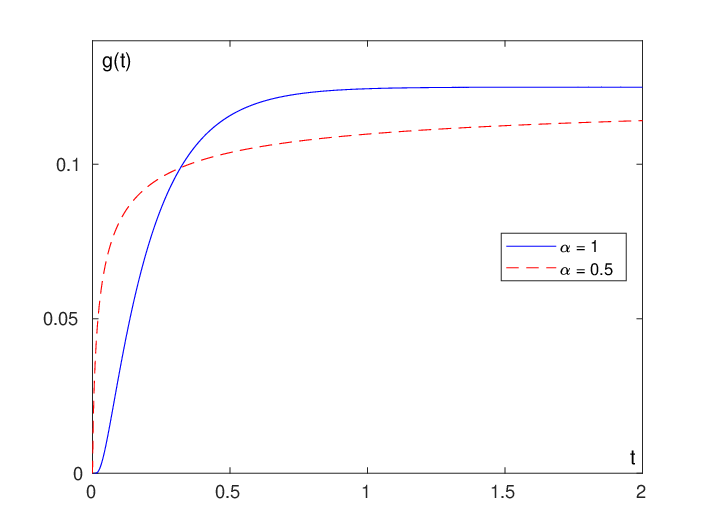
Refer to caption
Figure 3: The data gα​(t)g_{\alpha}(t).

Figure 3 shows the function g⁡(t)g(t) for both α=1\alpha=1 and α=12\alpha=\frac{1}{2}. In each case g⁡(t)g(t) goes to the same steady state value but how it approaches is quite different. In the case of the heat equation the effective steady state is reached long before the endpoint chosen here of T=2T=2. Indeed, by t=0.5t=0.5, 99% of the steady state value has been achieved and is typical of the behaviour expected by the exponential term in the solution representation when α=1\alpha=1. When α=12\alpha=\frac{1}{2} the situation is quite different; the Mittag-Leffler function decays only linearly for large (negative) values of the argument and so steady state is achieved much more slowly. In consequence, for α=1\alpha=1 only time measurements made for small tt offer any utility in providing information, but for α<1\alpha<1 this is not the case.

The model (1.1) has the positivity property; the nonhomogeneous forcing function and initial value are nonnegative and this implies the solution u⁡(x,t)u(x,t) be nonnegative for all (x,t)(x,t), see [9]. Thus the (exact) overposed flux values consisting of the outer normal derivative on ∂Ω\partial\Omega will be negative for all tt. In fact these values must start at 00 and monotonically decrease to the steady state value predicted by the equation −△​u=χ⁡(D)-\triangle u=\chi(D) with the same Dirichlet condition on ∂Ω\partial\Omega as imposed by (1.1). From equation (3.2) and the monotonicity of the Mittag-Leffler function on the negative real axis the term σα,n​(t):=1−Eα,1​(−λn​tα)\sigma_{\alpha,n}(t):=1-E_{\alpha,1}(-\lambda_{n}t^{\alpha}) is monotone and the range of this is within [0,1)[0,1) for all tt. Even if the time interval is truncated to [0,T][0,T], since λn→∞\lambda_{n}\to\infty linearly in nn, most of the modes will have the property that σα,n​(t)\sigma_{\alpha,n}(t) covers a substantial part of the range (0,1](0,1]. However, this will not be independent of α\alpha as the growth of Eα,1​(−λ​tα)E_{\alpha,1}(-\lambda t^{\alpha}) depends on α\alpha. The larger the α\alpha, the initially the slower, but finally the faster the decay of Eα,1​(−λ​tα)E_{\alpha,1}(-\lambda t^{\alpha}) to zero. Thus, as we have seen in Figure 3, the heat equation with α=1\alpha=1 will reach steady state faster than for α<1\alpha<1 and the smaller the α\alpha the longer it will take to reach steady state. Of course the high frequency modes (large λn\lambda_{n}) will reach steady state much faster and this is true for all α\alpha.

Refer to caption
Figure 4: Singular values of G′G^{\prime}.

Figure 4 displays the singular values σk\sigma_{k} of the operator (G′)∗∘G′(G^{\prime})^{*}\circ G^{\prime} for experiment E2​bE_{2b}. Note the obvious exponential decay of σk\sigma_{k} for all α\alpha. This is to be expected due to the extreme ill-conditioning of the problem. However, the rates do depend on α\alpha; the smaller the α\alpha the greater the decay rate and hence degree of ill-conditioning. Again, this must be expected as for small α\alpha the diffusion is initially extremely rapid and the transient information cannot be adequately captured. Thus, while all cases require g⁡(t)g(t) for small values of tt this is even more important the smaller the α\alpha. The slower growth of the profile g⁡(t)g(t) for larger tt cannot compensate. Although this seems anomalous at first glance, the factor 1−Eα,1​(−z)1-E_{\alpha,1}(-z) for large argument z=λn​tαz=\lambda_{n}t^{\alpha} approaches unity with behaviour c1z+c2z2+…\frac{c_{1}}{z}+\frac{c_{2}}{z^{2}}+\ldots where ck=ck​(α)c_{k}=c_{k}(\alpha). Hence for modest values of tt, say near t=1t=1 but large λn\lambda_{n} this is dominated by the first term with a rapidly diminishing contribution to further terms 1/z21/z^{2}, 1/z3​…1/z^{3}\ \ldots and so also offers very little information to be picked up from g⁡(t)g(t).

Note that while it is important to take a small step size initially in the measurement of g⁡(t)g(t) this need not be continued for the entire interval. Thus if we take say the first few measurements with d​t=0.001dt=0.001 then this can be steadily increased so that (say) over the last half of [0,T][0,T] we use a step size of d​t=0.1dt=0.1; with this the reconstructions differences will be imperceptible. In fact, the optimal measurement points {tk}\{t_{k}\} should be chosen to give approximately equal arc lengths of ur​(1,θ,t)=g⁡(t)u_{r}(1,\theta,t)=g(t). This will mean a far greater concentration of point for small values of tt and this effect will be stronger the smaller the α\alpha value.

Reconstructions are shown for experiments E1​bE_{1b} and E2​bE_{2b} and for α=0.1, 0.5, 1\alpha=0.1,\,0.5,\,1 in Figure 5. Here we took the initial step size in tt to be d​t=0.001dt=0.001.

Refer to caption
Refer to caption
Refer to caption
Refer to caption
Refer to caption
Refer to caption
Figure 5: E1​bE_{1b} (top) and E2​bE_{2b} (bottom) for α=0.1, 0.5, 1\alpha=0.1,\;0.5,\;1. δ=1%\;\delta=1\%.

These bear out the previous observations and with Figure 4. The differences are relatively small for α\alpha close to 11 but with a rapid deterioration, particularly in the higher frequency information, with decreasing α\alpha. Thus in E1​bE_{1b} the simple shaped-object has a virtually identical reconstruction for α=1/2\alpha=1/2 and α=1\alpha=1 - both within the variation expected with 1%1\%, noise but the reconstruction is clearly poorer for α=0.1\alpha=0.1 where we are only able to determine the rough size and placement. The similarity in E2​bE_{2b} is due to the small initial time steps taken; if instead we had to increase d​tdt to d​t=0.01dt=0.01 initially, then the difference between α=1/2\alpha=1/2 and α=1\alpha=1 would be much more evident.

What if we delay the flux measurements until a later time, that is we measure only over [T0,T][T_{0},T] for some T0>0T_{0}>0? There are certainly physical situations where this might be required. Note that Corollary 3.2 indicates uniqueness will still hold but the question is the resulting change in condition number. In Figures 6–8 we measure the flux data gℓ​(t)g_{\ell}(t) over incomplete intervals.

Figure 6 shows the expected outcome; a decrease in the ability to construct higher modes as short-time information is lost.

Refer to caption
Refer to caption
Refer to caption
Figure 6: Reconstructions for E2​bE_{2b} with data from [T0,T][T_{0},T] with T0=0\;T_{0}=0, T0=0.25\,T_{0}=0.25, T0=0.5\,T_{0}=0.5, α=0.9\;\alpha=0.9.

Figure 7 shows how this loss is greater for smaller α\alpha as should be expected from the above.

Refer to caption
Refer to caption
Figure 7: Results of experiments E2​bE_{2b} with data from [0.25,1][0.25,1], δ=1%\delta=1\% and α=0.5\alpha=0.5 (left), α=1\alpha=1 (right).

Figure 8 shows that when larger time values are missing the effect is greater for larger α\alpha and in particular, for the heat equation. This is again consistent with the above analysis and the fact that although the fractional diffusion takes longer to reach steady state, the later stages of the transient phase contains little information that can be used to reconstruct the source domain.

Refer to caption
Refer to caption
Figure 8: Results of experiments E2​bE_{2b} with data from [0,0.15][0,0.15], δ=1%\delta=1\% and α=0.5\alpha=0.5 (left), α=1\alpha=1 (right).

The explanation is clear from (3.2) and perhaps more apparent with the heat equation and the resulting exponential function E1,1E_{1,1} although the identical argument applies to the Mittag-Leffler function Eα,1E_{\alpha,1} albeit to a slightly different degree. For the term e−λn​te^{-\lambda_{n}t} to remain sufficiently large to contain extractable information we require the argument λn​t\lambda_{n}t to be sufficiently small. If λn<Λ\lambda_{n}<\Lambda and t>T0t>T_{0} then e−λn​t<e−Λ​T0<ϵe^{-\lambda_{n}t}<e^{-\Lambda T_{0}}<\epsilon for Λ<−ln(ϵ)/T0\Lambda<-\ln(\epsilon)/T_{0} showing that for a given ϵ\epsilon and value T0T_{0} we are restricted to a maximum Λ\Lambda; that is we cannot effectively use the nthn^{\rm th} eigenfunction mode in equation (3.2) if λn>Λ\lambda_{n}>\Lambda.

In summary, the optimal time-measurement intervals for recovering the source support DD in (1.1) depend strongly on α\alpha. Taking small initial time steps is advantageous in all cases but particularly important the smaller the value of α\alpha.

4.6 More than two measurement points

We should expect superior reconstructions with a greater number of observation points since we have additional data for which to average out measurement error. However, (3.9) shows much more is possible since we see that if the difference θi−θj\theta_{i}-\theta_{j} is near to a rational number pr\frac{p}{r} times π\pi with some r≤Mr\leq M, then the rthr^{\rm th} mode will be expressed very poorly from this combination. For a given MM, the more observation points taken, the greater the opportunity to avoid this situation. This allows an often significant increase in the resulting singular values and correspondingly a better inversion of G′G^{\prime} and hence of the reconstruction.

In experiment E2​cE_{2c}, we use four observation points.

q⁡(θ)=0.5+0.05​cos⁡θ+0.3​sin⁡2​θ,\displaystyle q(\theta)=0.5+0.05\cos{\theta}+0.3\sin{2\theta},
E2​c:\displaystyle E_{2c}: θ1=2332π,θ2=5732π,θ3=14π,θ4=3932π,\displaystyle\theta_{1}=\frac{23}{32}\pi,\ \ \theta_{2}=\frac{57}{32}\pi,\ \ \theta_{3}=\frac{1}{4}\pi,\ \ \theta_{4}=\frac{39}{32}\pi,
β=3×10⁻²,δ=1%,ϵ=δ/10.\displaystyle\beta=3\times 10^{-2},\ \delta=1\%,\ \epsilon=\delta/10.
Refer to caption
Refer to caption
Figure 9: Results of experiments E2​bE_{2b} (left) and E2​cE_{2c} (right) with α=0.9\alpha=0.9.

The result is shown in Figure 9 and by comparison with Figure 5 it is a considerable improvement over taking just two measurement points.

Acknowledgment

Both authors were supported by the National Science Foundation through award DMS-1620138. The second author was also supported by the Finnish Centre of Excellence in Inverse Problems Research through project 284715.

References

  • [1] Michele Caputo. Linear models of dissipation whose QQ is almost frequency independent – II. Geophys. J. Int., 13(5):529–539, 1967.
  • [2] Jin Cheng, Junichi Nakagawa, Masahiro Yamamoto, and Tomohiro Yamazaki. Uniqueness in an inverse problem for a one-dimensional fractional diffusion equation. Inverse Problems, 25(11):115002, 16, 2009.
  • [3] Mkhitar M Djrbashian. Integral Transformations and Representation of Functions in a Complex Domain [in Russian]. Nauka, Moscow, 1966.
  • [4] Mkhitar M. Djrbashian. Harmonic Analysis and Boundary Value Problems in the Complex Domain. Birkhäuser, Basel, 1993.
  • [5] F. Hettlich and W. Rundell. Identification of a discontinuous source in the heat equation. Inverse Problems, 17(5):1465–1482, 2001.
  • [6] Frank Hettlich and William Rundell. Iterative methods for the reconstruction of an inverse potential problem. Inverse Problems, 12(3):251–266, 1996.
  • [7] Bangti Jin, Raytcho Lazarov, and Zhi Zhou. An analysis of the L1 scheme for the subdiffusion equation with nonsmooth data. IMA J. Numer. Anal., 36(1):197–221, 2016.
  • [8] Bangti Jin and William Rundell. A tutorial on inverse problems for anomalous diffusion processes. Inverse Problems, 31(3):035003, 40, 2015.
  • [9] Yikan Liu, William Rundell, and Masahiro Yamamoto. Strong maximum principle for fractional diffusion equations and an application to an inverse source problem. Fract. Calc. Appl. Anal., 19(4):888–906, 2016.
  • [10] Francesco Mainardi, Antonio Mura, and Gianni Pagnini. The MM-Wright function in time-fractional diffusion processes: a tutorial survey. Int. J. Differ. Equ., pages Art. ID 104505, 29, 2010.
  • [11] Kenichi Sakamoto and Masahiro Yamamoto. Initial value/boundary value problems for fractional diffusion-wave equations and applications to some inverse problems. J. Math. Anal. Appl., 382(1):426–447, 2011.
  • [12] Stefan G. Samko, Anatoly A. Kilbas, and Oleg I. Marichev. Fractional Integrals and Derivatives. Gordon and Breach Science Publishers, Yverdon, 1993.