Robust Monitoring of Time Series
with Application to Fraud
Detection00footnotetext: Peter Rousseeuw,
Department of Mathematics, University
of Leuven, Belgium. Domenico Perrotta, Joint
Research Centre, Ispra, Italy. Marco Riani,
Department of Economics, University of Parma,
Italy. Mia Hubert, Department of Mathematics,
University of Leuven, Belgium.
Peter Rousseeuw and Mia Hubert gratefully
acknowledge the support by project C16/15/068
of Internal Funds KU Leuven. The work of
Domenico Perrotta was supported by the Project
“Automated Monitoring
Tool on External Trade Step 5” of the Joint
Research Centre and the European Anti-Fraud
Office of the European Commission, under the
Hercule-III EU programme.
In this paper, references to specific countries
and products are made only for purposes of
illustration and do not necessarily refer to
cases investigated or under investigation by
anti-fraud authorities.
Abstract
Time series often contain outliers and level shifts or structural changes. These unexpected events are of the utmost importance in fraud detection, as they may pinpoint suspicious transactions. The presence of such unusual events can easily mislead conventional time series analysis and yield erroneous conclusions. A unified framework is provided for detecting outliers and level shifts in short time series that may have a seasonal pattern. The approach combines ideas from the FastLTS algorithm for robust regression with alternating least squares. The double wedge plot is proposed, a graphical display which indicates outliers and potential level shifts. The methodology was developed to detect potential fraud cases in time series of imports into the European Union, and is illustrated on two such series.
Keywords: alternating least squares, double wedge plot, level shift, outliers.
1 Introduction
When analyzing time series one often encounters unusual events such as outliers and structural changes, like those in Figure 1. Both series track trade volumes, and were extracted from the official trade statistics in the COMEXT database of Eurostat. This database contains monthly trade volumes (aggregated over several transactions, possibly involving different traders) of products imported in the European Union (EU) in a four-year period. The plot titles in Figure 1 specify the code of the traded product in the EU Combined Nomenclature classification (CN code), the country of origin, and the destination (a member state of the EU). The CN code determines whether the volumes are expressed in tons of net mass and/or other units (liters, number of items, etc.), the rate of customs duty applied, and how the goods are treated for statistical purposes. The data quality is quite heterogeneous across countries and products, but some macroscopic outliers (manifest errors) have already been removed or corrected by statistical authorities and customs services.
 |
 |
| (a) | (b) |
Both of these time series exhibit a downward level shift. Knowing when such structural breaks occur is important for fraud detection. For instance, a sudden reduction in trade volume may coincide with an increase for a related product or another country of origin, which could indicate a misdeclaration with the intent of deflecting customs duties.
There are many products and countries of origin in the CN classification, but not all of these combinations occur and the number of products at risk of fraud is relatively small. Still, the number of relevant combinations of a product at fraud risk, a country of origin and a country of destination is around 16,000. As a result, every month around 16,000 time series need to be analyzed for anti-fraud purposes. This requires an automatic approach that is able to report accurate information on outliers and the positions and amplitudes of level shifts, and that runs fast enough for that time frame. The method proposed in this paper meets those objectives, and provides a graphical display that can be looked at whenever the automatic monitoring system detects a significant level shift. Our method follows the approach which first computes a robust fit to the majority of the data and then detects outliers by their large residuals, as described in the review paper (Rousseeuw and Hubert, 2018).
A different statistical approach to monitor international trade data for fraud was proposed by Barabesi et al. (2016) who tested whether the distribution of trade volumes follows the Newcomb-Benford law. In the current paper we also take the time sequence of the trades into account. We will focus on a parametric approach to estimate level shifts, which differs from the nonparametric smoothing methods in Fried and Gather (2007) or robust methods for REGARIMA models (Bianco et al., 2001). A popular technique is the X13 ARIMA-SEATS Seasonal Adjustment methodology (Findley et al., 1998; U.S. Census Bureau, 2017). X-13 is based on automatic fitting of ARIMA models and includes detection of additive outliers and level shifts. We will compare our results with those of X-13 in Section 5. See also Galeano and Peña (2013) for a review of robust modeling of linear and nonlinear time series.
Although this paper was motivated by the need to analyze many short time series of trade data, we will describe the methodology more generally so it can be applied to other types of time series that may be longer and can be modeled with more parameters.
The structure of the paper is as follows. In Section 2 we introduce our model and methodology for robustly analyzing a time series which contains a trend, a seasonal component and possibly a level shift in an unknown position, as well as isolated or consecutive outliers. In Section 3 we illustrate the proposed approach using the well-known airline data (Box and Jenkins, 1976), as well as contaminated versions of it in order to test the ability of the method to detect anomalies. In this section we also introduce the double wedge plot, which visualizes the presence of a level shift and outliers. In Section 4 we apply our methodology to the time series in Figure 1. Section 5 compares our results to those obtained by a nonparametric method and to X-13. The case where more than one level shift occurs is discussed in Section 6. Section 7 concludes, and the Appendix proves a result about our algorithm.
2 Methodology
2.1 The model
The time series (for ) we will consider may contain the following terms:
- 1.
a polynomial trend, i.e. ;
- 2.
a seasonal component, i.e.
(1) When this is periodic with a one-year period, corresponds with a six-month period etc. We assume the amplitude of the seasonal component varies over time in a polynomial way, i.e. ;
- 3.
a level shift in an unknown time point , i.e. with the indicator function.
The general model is thus of the form
| (2) | |||||
One may assume that the irregular component of the non-outliers is a stationary random process with and . Let us collect all unknown parameters in a vector of length . Then model (2) can be written as
with . The model does not need to contain all of these components, as some coefficients can be zero.
2.2 The nonlinear LTS estimator
Model (2) is nonlinear in the parameters , , and . As there may be outliers in the time series, we propose to estimate by means of the nonlinear least trimmed squares (NLTS) estimator (Rousseeuw, 1984; Stromberg and Ruppert, 1992; Stromberg, 1993):
| (3) |
where and is the -th smallest squared residual . Our default choice for is .
The -consistency and asymptotic normality of NLTS were studied by Čížek (2005); Čížek (2008). To compute the estimator, we propose to combine ideas from the FastLTS algorithm for robust linear regression (Rousseeuw and Van Driessen, 2006) with the alternating least squares (ALS) method.
We first describe how we use the alternating least squares procedure. We temporarily assume that the estimated shift time is fixed, and that we want to solve (3) for a subset of the with at least observations, at least one of which is to the left of and at least one of which is equal or to the right of . We denote the indices of the subset as with , where must overlap with as well as . These conditions are required to make the parameters in (2) identifiable from the subset . We then go through the following steps:
- 1.
[Initialization] Set for . Then a part of (2) drops out, leaving
(4) which is linear in the parameters , , and . By applying linear LS to the subset , we obtain the initial estimates , , and .
- 2.
[Iteration] For repeat the following steps:
- •
[ALS step A] Let in which the coefficients and come from the previous step. Keeping fixed yields the model
(5) which is linear in the parameters , , and . We then apply LS using only the observations in the subset , yielding the estimates , and .
- •
[ALS step B] Keeping the estimated coefficients , and from the previous step fixed yields the model
(6) which is linear in the parameters and . We then apply LS using only the observations in the subset , yielding the estimates and . Then we go back to ALS step A.
- •
Let be the vector of coefficients after iteration step . We repeat the above steps until is below a threshold, or a maximal number of iterations (say 50) is attained. Here is the Euclidean norm.
In words, ALS solves the nonlinear LS problem of fitting (2) to the data set by alternating between the solution of two linear LS fits, (5) and (6).
Our goal is to solve the nonlinear LTS problem (3). A basic tool for linear LTS is the C-step (Rousseeuw and Van Driessen, 2006) which we now generalize to the nonlinear setting.
[C-step] Start from a subset to which we fit obtained by applying ALS. Then compute the residuals for the whole time series, that is, for and not just for . Next retain the observations with smallest squared residuals, yielding the new subset . Then apply ALS to , yielding a new fit . It is shown in the Appendix that the new fit is guaranteed to have a lower objective function than the old fit . It is possible to iterate the C-step until convergence, which will occur in a finite number of steps.
Using these building blocks, we now describe the entire algorithm to compute the NLTS fit to the model (2). Let be the ordered indices of the possible positions of the level shift, for example the set for some . The algorithm then consists of the following steps.
- 1.
Loop over all where and do:
- (a)
Temporarily set .
- (b)
Now loop over ranging from 1 to the number of trial subsets , and do:
- i.
Construct an elemental subset containing different observations. This subset should contain the index , one observation with and observations drawn at random from the whole time series. Note that we impose that belongs to because the purpose of step 1 is to select the most suitable .
- ii.
Run the initialization and ALS steps described above on , keeping fixed. Then take two C-steps. [Two C-steps is enough at this stage, in line with the results of Rousseeuw and Van Driessen (2006).] If a singular solution is obtained during the computations, restart without increasing .
The choice of is a compromise since the expected number of outlier-free subsets is proportional to but the computation speed is inversely proportional to . In our experiments we found that was sufficient to obtain stable results.
- i.
- (c)
Consider only the nbest elemental subsets (among the that were tried) that yielded the lowest objective function so far. Apply C-steps to them until convergence and store these nbest solutions. In our examples we found that setting nbest to 10 worked well.
- (d)
If also start from the nbest elemental sets found when investigating , but this time setting . Apply C-steps to them until convergence.
- (e)
Take the fit with the lowest objective among these candidates, and denote it by .
- (f)
Store the corresponding scaled residuals
(7)
- (a)
- 2.
Retain overall best solution. Among the fits for take the one with lowest objective function and denote it by .
For estimating the scale of the error term we can use . But since this sum of squares only uses the most central residuals, the estimate needs to be rescaled. The variance of a truncated normal distribution containing the central portion of the standard normal isby equation (6.5) in (Croux and Rousseeuw, 1992). Therefore we compute
(8) Note that this makes consistent, but not yet unbiased for small samples. Therefore we include the finite-sample correction factor from Pison et al. (2002) in our final scale estimate .
- 3.
Locally improving the shift position estimate. The previous steps have yielded an estimate of the position of the level shift, but it may be imprecise. For instance, it may happen that the -subset underlying does not itself contain the time points or . In order to improve the estimate we check in its vicinity as follows:
- •
Take a window around . For each in , we replace by while keeping the other coefficients from and the scale estimate . Compute the residuals from these coefficients and let with the Huber function
In our simulations and the analysis of international trade time series (of the kind given in Figure 1) the best results were obtained with equal to 1.5 or 2. In our implementation the defaults are and a window of width 15.
- •
Our final is the in with lowest . If it is different from the estimate we had before, we recompute the scaled residuals.
- •
- 4.
Weighted step. We apply the univariate outlier detection procedure described in (Gervini and Yohai, 2002) and (Agostinelli et al., 2015) to the scaled residuals . By default we use the 99% confidence level. Alternatively, one could use the thresholds obtained in Salini et al. (2015).
- 5.
Final fit. We apply nonlinear LS to all the points that have not been flagged as outliers in the previous step, starting from the initial estimate and keeping fixed. For this we can iterate ALS steps until convergence. The standard errors obtained in the last two ALS steps can be used for inference.
Note that must be at least the number of parameters in the model for identifiability. When is as low as this means . However, for stability it is often recommended that , see e.g. Rousseeuw and Leroy (1987). The Matlab code of the algorithm can be downloaded from /www.riani.it/rprh/ . In the following sections we will apply it to several data sets.
3 Airline data and the double wedge plot
The airline passenger data, given as Series G in Box and Jenkins (1976), has often been used in the time series analysis literature as an example of a nonstationary seasonal time series. It consists of monthly total numbers of airline passengers from January 1949 to December 1960. Box and Jenkins developed a two-coefficient time series model of factored form that is now known as the airline model. In this section we will analyze these data using our method, and then contaminate the data in various ways to see how the method reacts.

Uncontaminated data. We fit the data by model (2) with , and . This means that we assume a quadratic trend, a quarterly seasonal component, and a quadratically varying amplitude. The resulting NLTS fit (3) closely follows the data, as can be seen in Figure 2. In this example no data point has been flagged as outlying. From the standard errors (not shown) we conclude that all coefficients are significant except for the height of the level shift.

Contamination 1. We now contaminate the series by adding three groups of outliers, yielding the blue curve in the bottom panel of Figure 3. More precisely, the value 300 is subtracted from all responses in the interval while 300 is added on and 400 is subtracted on . The fitted values (dotted curve) from NLTS closely follow the observed values for the regular observations. The flagged outliers are indicated by red crosses, whose size is proportional to the absolute magnitude of their residual. We see that all the outliers we added are clearly recognized as such, and they were not used to estimate the coefficients in the weighted step. Only a few regular observations received an absolute residual slightly above the cutoff value.
The top panel of Figure 3 is a byproduct of the algorithm, and is useful for visualizing the presence of (groups of) outliers and a level shift. The first step of the algorithm ranges over all potential positions of a level shift. These tentative positions are on the vertical axis. For any we plot the absolute scaled residuals given in (7), in all of the times on the horizontal axis. The color in the plot depends on the size of that absolute residual and ranges from black (large residuals) over red and yellow to white (small residuals). The color scale is at the right of the plot. Scaled residuals larger than are shown as if they were , so that even a very far outlier cannot affect the color coding. In the same spirit, uninformative scaled residuals smaller than are shown as if they were 0, so in white. Of course the user can easily modify these default choices.
Outliers have a large absolute scaled residual from the robust fit, so in this plot isolated outliers will appear as dark vertical lines, and groups of consecutive outliers as dark vertical bands. In this example we clearly see the contamination. The regular observations with scaled residual slightly above 2.5 do not stand out as they are in light yellow.
Contamination 2. In the second contamination setting we introduce a persistent level shift and three isolated outliers, two of which lie in the proximity of the level shift which makes the problem harder. For this we added the value 1300 to all responses from onward, at the response is lowered by 800, at by 600, while at and we added an additional 800.

The bottom panel of Figure 4 shows the observed and fitted values. Again all inserted outliers are clearly detected, and a few regular observations have small crosses indicating that their scaled absolute residual was slightly above 2.5 .
The plot of the absolute scaled residuals in the top panel of Figure 4 now looks more eventful with two dark triangles. Together these ‘wedges’ signal a level shift. To understand this effect, let us assume that the true level shift is at position and the algorithm is in the process of checking the candidate . Then the algorithm will treat the at as outliers and the resulting robust fit (still for that ) will show consecutive outliers. Similarly, when the algorithm tries to the right of , the best solutions will show outliers. As a result, when approaching the true level shift position from the left the scaled residuals we are monitoring will form a dark upward-pointing wedge, and to the right of the true we obtain an analogous wedge pointing downward. In the top panel of Figure 4. we observe two opposite wedges tapering off in the proximity of the true level shift position, around . In this region we observe a small rectangle (centered at position 68) bridging the two wedges. The rectangle is due to the two outliers in the proximity of the level shift. The isolated outlier at position 45 yields a single dark vertical line like those in Figure 3.
 |
 |
| (a) | (b) |
Panel (a) of Figure 5 shows the boxplots of the objective function attained by the best solutions in step 1(e) of the algorithm. It is thus also a free byproduct of the estimation. If a level shift is present in the central part of the time series, this plot will typically have a shape. In this example the lowest values of the trimmed sum of squared residuals occur in the time range 60-80. The continuous curve which connects the lowest objective value for each reaches its global minimum at . However, the curve is quite bumpy in that region, with several local minima and a near-constant stretch on 67-70, so the position of the minimum is not precise. This kind of situation motivated the local improvement in step 3 of the algorithm. Panel (b) of Figure 5 shows as a function of the tentative position (with the Huber function with ) on the interval 53-82. This curve has a much better determined minimum, in fact at , confirming the benefit of the local improvement step.

Contamination 3. In the final contaminated dataset we inserted a level shift and a group of consecutive outliers following it. To complicate things even more, we also put in a stretch of contamination to the left of the level shift, as well as an isolated outlier. The bottom panel of Figure 6 shows the robust fit, which succeeded in recovering the structure and flagging the outliers. In the top panel of Figure 6 we see the typical double wedge pattern indicating a level shift. The two reddish bands flag the groups of consecutive outliers, whereas the single line corresponds to the isolated outlier at . In this example the thick end of the upper wedge is yellow, so the absolute scaled residuals are not as large there. This part corresponds to a tentative level shift of around 100, which is very far from the true one, and in such cases the fit may indeed be quite different.
4 Analysis of trade data
Our main goal is to analyze the many short time series of trade described in Section 1. After trying several model specifications in the class (2) we found that the best results were obtained by using a linear trend, two harmonics, and one parameter to model the varying amplitude of the seasonal component, that is, , and . Note that this yields parameters including the position and height of a potential level shift, which is not too many compared to the length of the time series (). As an example we now apply our method to the time series in Figure 1.
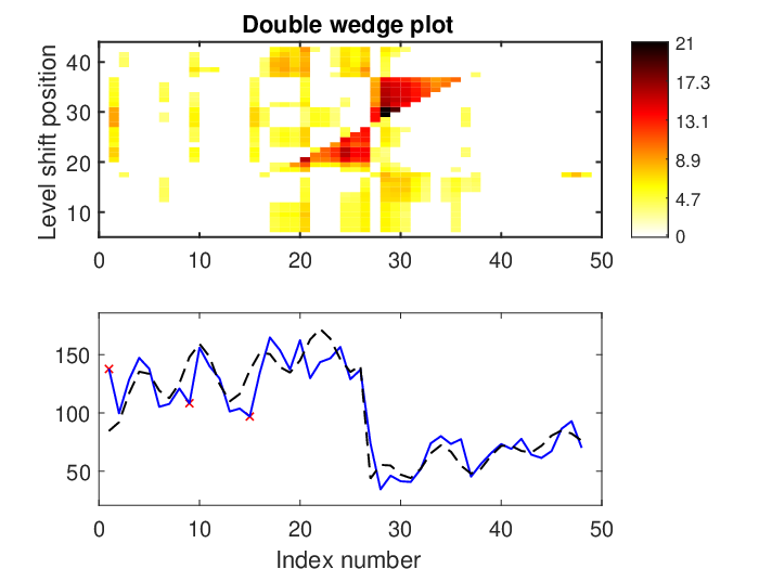
The robust fit to series P12119085-KE-GB (bottom panel of Figure 7) suggests three moderate outliers in positions 1, 9 and 15. The fit closely matches the level shift which is therefore well captured. The double wedge plot in the top panel of Figure 7 has two wedges which point to a level shift position around 27-28. The local refinement step selects position .
Columns 2–4 of Table 1 show the coefficients of the final fit together with their -statistics and -values. Most coefficients are significant, and in particular the -statistic of the height of the level shift is quite large with . This drop looks anomalous because in the period considered, Kenya was the only country of the East African Community (EAC) paying high European import duties on flowers and related products including CN 12119085. On the other hand, Kenya is the third largest exporter of cut flowers in the world. One would therefore check for a simultaneous upward level shift in an EAC country not paying import duties, which could point to a misdeclaration of origin.
| P12119085_KE_GB | P17049075_UA_LT | |||||
|---|---|---|---|---|---|---|
| Coeff | -stat | -values | Coeff | -stat | -values | |
| 115.27 | 25.6 | 0 | 55.14 | 14.3 | 0 | |
| 1.59 | 5.80 | 0 | 0.90 | 4.52 | 0 | |
| -2.83 | -0.72 | 0.47 | 15.55 | 3.75 | 0.00056 | |
| -12.42 | -2.65 | 0.012 | 3.61 | 0.85 | 0.40 | |
| -9.07 | -1.95 | 0.059 | -32.50 | -7.64 | 0 | |
| -22.60 | -4.80 | 0 | -16.06 | -3.72 | 0.00061 | |
| -0.016 | -3.72 | 0.00061 | -0.023 | -12.1 | 0 | |
| -112.62 | -14.7 | 0 | -79.41 | -13.9 | 0 | |
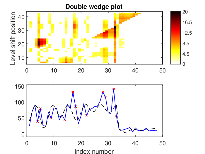
Figure 8 shows the results for the second series, P17049075_UA_LT. The double wedge plot indicates the presence of a level shift around position 35. The local refinement yields the position . Interestingly, there is a reddish line right before the level shift. This is due to an outlier in position 32 which gets a red cross in the bottom panel of the figure. The double wedge plot also reveals a yellow strip at positions 29 and 30, indicating two less extreme outliers. Finally, the plot also shows some small reddish areas that correspond to local irregularities, for instance observations 4, 5, 17 and 18 which are flagged as outliers in the bottom panel. Columns 5–7 of Table 1 list the coefficients of the final fit. Also here most coefficients are strongly significant.
In this case the level shift might point to a different type of violation. The market of sugar and high-sugar-content products, such as CN code 17049075, is very restricted and regulated. The EU applies country-specific quotas for these products, with lower import duty for imports below the quota and a higher duty beyond this limit (tariff rate quotas). Therefore, it would be in an exporter’s interest to circumvent the quota by mislabeling this product as a somewhat related product that is not under surveillance. In this situation one would check for upward level shifts in related products from the same country.
Note that the -values and -values provided by LTS can help select a model. Table 1 fits model (2) with (linear trend), (two harmonics), and (the amplitude varies linearly). If we increase we find that a quadratic trend is insignificant, and the same for increasing . The -values indicate that there is enough evidence for a 6-month seasonal effect but are less clear on the question whether should be increased further for these short time series. In any case the detection of the level shift turns out to be stable as a function of here.
5 Comparison with other methods
We now compare our results with those obtained by the nonparametric method introduced by Fried (2004) and Fried and Gather (2007) for robust filtering of time series. For this we used the function robust.filter from the R package robfilter of Fried et al. (2012). The robust fitting methods are applied to a moving time window of size width, which needs to be an odd number.
| Window width | Level shift position(s) | Outlier position(s) |
|---|---|---|
| 3 | - | [ 10, 16, 17, 37, 38, 46, 47 ] |
| 5 | - | [ 16, 17, 18, 47 ] |
| 7 | [ 27 ] | [ 17, 18 ] |
| 9 | [ 27, 37 ] | - |
| 11 | [ 27 ] | - |
| Window width | Level shift position(s) | Outlier position(s) |
|---|---|---|
| 3 | - | [ 2, 15, 44 ] |
| 5 | - | [ 15, 16, 17, 28, 30, 31, 33, 39, 40, 41 ] |
| 7 | - | [ 30, 31, 33, 34 ] |
| 9 | - | [ 30, 31, 33, 34, 35 ] |
| 11 | [ 30 ] | [ 32 ] |
Tables 2 and 3 report the position of the level shift(s) and outlier(s) detected with all default options and various choices of window widths. We also tested different robust choices for the trend and scale estimation and some values for the adapt option which adapts the moving window width, with similar results.
 |
 |
| (a) | (b) |
Figures 9(a) and (b) show the resulting fits obtained by the nonparametric filter, for widths giving rise to the detection of a level shift (width for P_12119085_KE_GB and width for P_17049075_UA_LT). In the first series we see that the level shift is detected well for the appropriate width, but the fit itself is not as tight. Also in the second series a reasonable level shift position is found but the fit is not that close to the series. This can be explained by the fact that a nonparametric method has no prior knowledge about the data as it has to work on any data set, whereas our parametric model benefits from knowledge about the typical behavior of trade time series. In that sense the comparison is not entirely fair.
We also run the well-known X-13 ARIMA-SEATS method (Findley et al., 1998; U.S. Census Bureau, 2017) on both trade time series, by means of the R package seasonal (Sax, 2017) which interfaces X-13. This method fits an ARIMA model with a seasonal component. In additional to the coefficients required for the ARIMA model, X-13 has additional parameters for level shifts, one at each time point , plus parameters for additive outliers (AO). Their coefficients are estimated by stepwise regression, so most of them remain zero. For detecting isolated outliers, i.e. outliers surrounded by non-outlying values, this approach works quite well.

Figure 10 shows the X-13 fit to the trade series P12119085_KE_GB in the lower panel, with the LTS fit in the upper panel for comparison. Figure 11 does the same for P17049075_UA_LT. The blue curves are the time series, and the fits are in black. In both cases X-13 does detect the level shift. It obtains the model (0 1 1) which only has a moving average and no seasonal component. As a result its forecast (shown in red) has no seasonal component either. Note that in Figure 10 the 90% tolerance band around the forecast is much wider for X-13 than for LTS.

Let us now return to the airline data with contamination 1 described in Section 3. The results of LTS were shown in Figure 3. We now apply X-13 to it. The R-code and output are available in Section A.1 of the Supplementary Material. The model found by X-13 is ARIMA with (1 1 0)(0 1 0) whereas for the uncontaminated airline data it was (0 1 1)(0 1 1). In this example the X-13 fit has 7 nonzero coefficients describing level shifts, and 1 nonzero coefficient for an AO outlier. The bottom panel of Figure 12 shows the time series and the X-13 fit which accommodates the outliers. On the other hand, the LTS fit in the top panel follows the pattern of the majority of the data, so the outliers have large residuals from it. Also the forecasts are quite different: those of LTS increase and have a narrow tolerance band, while those of X-13 slightly decrease and have wide tolerance bands. For the uncontaminated airline data (that is, without outliers) the forecasts and tolerance bands of LTS and X-13 were very similar.

Note that X-13 fits each set of consecutive outliers by a level shift at the start and a level shift afterward. That description is indeed equivalent to the consecutive outliers representation. Our point is that accommodating the outliers gives a close fit to the observed time series, but as we see here it can inflate the forecast band.
On the airline data without outliers, X-13 automatically log transforms the data before fitting it. On the airline data with contamination it does not, because the time series contains at least one negative value. (Other transformations would be possible, but in automatic mode X-13 only considers the log transform.) In this example the negative values were due to outliers, but in fact many trade time series in the EU database have at least one zero value, correctly reflecting that a certain product was not imported for a month, which will also prevent X-13 from transforming the data.
To investigate this issue further, we looked at two ways to make the contaminated airline data positive. The first was to add a constant so that the minimum of the contaminated time series becomes 1 (we also tried 5, 10 and 50). The second was to truncate the series from below at 1 (or 5, 10, 50) so the downward outliers of contamination 1 remain visible. However, in none of these cases did X-13 carry out a logarithmic transform, indicating that its transformation criterion was affected by the outliers.
Also note that the outliers have a large magnitude in this example. In response to a referee request we also provide an example with a level shift that is smaller than the seasonal component, in Section A.2 of the Supplementary Material.
6 The case of several level shifts
Our basic model (2) only covers the situation where at most one level shift occurs, which is a reasonable assumption for short time series. When several level shifts can occur, we first apply our approach to the original time series. If it detects a level shift we can modify the time series by undoing the break, that is, subtract from all to the right of the level shift, after which one can search for the next level shift, and so on. A detailed example of this procedure is shown in subsection A.3 of the Supplementary Material.
7 Conclusions and outlook
We have introduced a new robust approach to model and monitor nonlinear time series with possible level shifts. A fast algorithm was developed and applied to several real and artificial datasets. We also proposed a new graphical display, the double wedge plot, which visualizes the possible presence of a level shift as well as outliers. This graph requires no additional computation as it is an automatic by-product of the estimation. Our approach thus allows to automatically flag outlying measurements and to detect a level shift, which is important in fraud detection as these may be indications of unauthorized transactions. At the European Joint Research Centre, this methodology was validated by comparing its results to those of visual inspection of many trade series by subject-matter experts.
Supplementary Material
The supplementary material to this paper contains some R code and worked-out examples.
Appendix
Here we prove that a C-step (as used in the first step of the NLTS algorithm) can only decrease the LTS objective function.
Let be the current -subset with its corresponding nonlinear LS coefficients and objective function .
Now consider , the -subset which contains the observations with smallest squared residual with respect to . Then by construction
| (9) |
The ALS step A then yields . Since it is the LS solution of the linear model (5),
| (10) |
Next, ALS step B yields with
| (11) |
References
References
- Agostinelli et al. (2015) Agostinelli, C., Leung, A., Yohai, V., Zamar, R., 2015. Robust estimation of multivariate location and scatter in the presence of cellwise and casewise contamination. Test 24, 441–461.
- Barabesi et al. (2016) Barabesi, L., Cerasa, A., Perrotta, D., Cerioli, A., 2016. Modelling international trade data with the Tweedie distribution for anti-fraud and policy support. European Journal of Operational Research 258, 1031–1043.
- Bianco et al. (2001) Bianco, A. M., GarcÃa Ben, M., MartÃnez, E. J., Yohai, V. J., 2001. Outlier detection in regression models with ARIMA errors using robust estimates. Journal of Forecasting 20 (8), 565–579.
- Box and Jenkins (1976) Box, G. E. P., Jenkins, G. M., 1976. Time Series Analysis: Forecasting and Control. Holden Day, San Francisco.
- Čížek (2005) Čížek, P., 2005. Least trimmed squares in nonlinear regression under dependence. Journal of Statistical Planning and Inference 136, 3967–3988.
- Čížek (2008) Čížek, P., 2008. General trimmed estimation: robust approach to nonlinear and limited dependent variable models. Econometric Theory 24 (6), 1500–1529.
- Croux and Rousseeuw (1992) Croux, C., Rousseeuw, P. J., 1992. A class of high-breakdown scale estimators based on subranges. Communications in Statistics - Theory and Methods 21, 1935–1951.
- Findley et al. (1998) Findley, D. F., Monsell, B. C., Bell, W. R., Otto, M. C., Chen, B. C., 1998. New capabilities of the X-12-ARIMA seasonal adjustment program. Journal of Business and Economic Statistics 16, 127–177.
- Fried (2004) Fried, R., 2004. Robust filtering of time series with trends. Journal of Nonparametric Statistics 16 (3-4), 313–328.
- Fried and Gather (2007) Fried, R., Gather, U., 2007. On rank tests for shift detection in time series. Computational Statistics & Data Analysis 52 (1), 221–233.
- Fried et al. (2012) Fried, R., Schettlinger, K., Borowski, M., 2012. Package ‘robfilter’. CRAN, URL https://CRAN.R-project.org/package=robfilter .
- Galeano and Peña (2013) Galeano, P., Peña, D., 2013. Finding outliers and unexpected events in linear and nonlinear possible multivariate time series data. In: Becker, C., Fried, R., Kuhnt, S. (Eds.), Robustness and Complex Data Structures. Festschrift in Honour of Ursula Gather. Springer, pp. 255–273.
- Gervini and Yohai (2002) Gervini, D., Yohai, V. J., 2002. A class of robust and fully efficient regression estimators. Annals of Statistics 30, 583–616.
- Pison et al. (2002) Pison, G., Van Aelst, S., Willems, G., 2002. Small sample corrections for LTS and MCD. Metrika 55, 111–123.
- Rousseeuw (1984) Rousseeuw, P., 1984. Least median of squares regression. Journal of the American Statistical Association 79, 871–880.
- Rousseeuw and Hubert (2018) Rousseeuw, P., Hubert, M., 2018. Anomaly detection by robust statistics. WIREs Data Mining and Knowledge Discovery e1236.
- Rousseeuw and Leroy (1987) Rousseeuw, P., Leroy, A., 1987. Robust Regression and Outlier Detection. Wiley-Interscience, New York.
- Rousseeuw and Van Driessen (2006) Rousseeuw, P., Van Driessen, K., 2006. Computing LTS regression for large data sets. Data Mining and Knowledge Discovery 12, 29–45.
- Salini et al. (2015) Salini, S., Cerioli, A., Laurini, F., Riani, M., 2015. Reliable robust regression diagnostics. International Statistical Review 84, 99–127.
- Sax (2017) Sax, C., 2017. Package ‘seasonal’: R Interface to X-13-ARIMA-SEATS. CRAN, URL https://CRAN.R-project.org/package=seasonal .
- Stromberg (1993) Stromberg, A., 1993. Computation of high breakdown nonlinear regression parameters. Journal of the American Statistical Association 88, 237–244.
- Stromberg and Ruppert (1992) Stromberg, A., Ruppert, D., 1992. Breakdown in nonlinear regression. Journal of the American Statistical Association 87, 991–997.
- U.S. Census Bureau (2017) U.S. Census Bureau, 2017. X-13ARIMA-SEATS Reference Manual, Version 1.1. URL http://www.census.gov/srd/www/x13as .
SUPPLEMENTARY MATERIAL
A.1 R-code for the airline data with contamination 1
> library("seasonal")
> library("forecast")
> y = AirPassengers
> y[50:55]   = y[50:55]-300
> y[122:127] = y[122:127]+300
> y[130:134] = y[130:134]-400
> out = seas(y, forecast.save = "forecasts")
> summary(out)

Coefficients:
                    Estimate Std. Error z value Pr(>|z|)
LS1953.Feb        -294.29555    6.88904 -42.719  < 2e-16 ***
LS1953.Aug         304.98444    6.88904  44.271  < 2e-16 ***
AO1959.Feb         310.47628    7.17862  43.250  < 2e-16 ***
LS1959.Mar         329.79392   11.04369  29.863  < 2e-16 ***
LS1959.Aug        -285.79555    6.88904 -41.486  < 2e-16 ***
LS1959.Oct        -404.90220    6.88904 -58.775  < 2e-16 ***
LS1960.Mar         385.12429   14.05921  27.393  < 2e-16 ***
LS1960.Apr          47.91993   10.15210   4.720 2.36e-06 ***
AR-Nonseasonal-01   -0.30043    0.08324  -3.609 0.000307 ***
---
SEATS adj.  ARIMA: (1 1 0)(0 1 0)  Obs.: 144  Transform: none

> forec = series(out, c("forecast.forecasts", "s12"))
> forec[1:144,1] = y
> plot(forec[,1],ylim=c(-100,800),col="blue")
> fit = trend(out) + forecast::seasonal(out)
> lines(fit,col="black")
> lines(forec[,2],col="red") # forecast
> lines(forec[,3],col="red")
> lines(forec[,4],col="red")
A.2 Effect of a small level shift
For this example the time series has length and it is generated according to model (2) with , , . In particular , , and . There is one level shift of height at time . The error term is generated with a signal to noise ratio of 20.

All the components in Figure 13 are shown using the same vertical scale so their relative size can be seen. The trend is increasing but appears horizontal if we compare it to the magnitude of the other components. We see that the level shift is smaller than the seasonal component, and similar in size to the spread of the error term (called “irregular” in the plot). The time series will be made available on /www.riani.it/rprh/ .
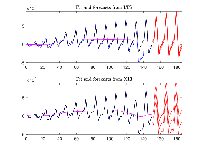
After generating this time series we also create a stretch of outliers by subtracting 29,000 from the values at times in . The top panel of Figure 14 shows the result of the LTS procedure, with the time series (blue), the estimated trend including the estimated level shift (purple), the overall fit (black) and the forecast (red). The level shift is clearly visible, and the outliers stand out by their sizeable residual (look at in this plot) for in .
The bottom panel shows the X-13 fit, which does not detect the level shift. Instead there is a mild increase in the X-13 trend where the level shift takes place, followed by a mild decrease in the vicinity of the stretch of outliers. The X-13 forecast is stationary, whereas the LTS forecast has increasing seasonal fluctuations in line with the underlying model. The tolerance band around the forecast is much wider for X-13 than for LTS.
A.3 More than one level shift
We now consider an example with two level shifts. Starting from the original airline data, we subtract 100 from the values at times in and add 200 at the times in which creates level shifts at times 31 and 100.
 |
 |
| (a) | (b) |
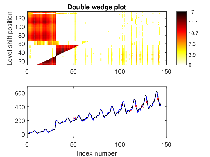
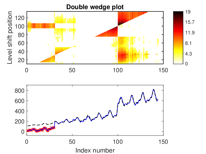
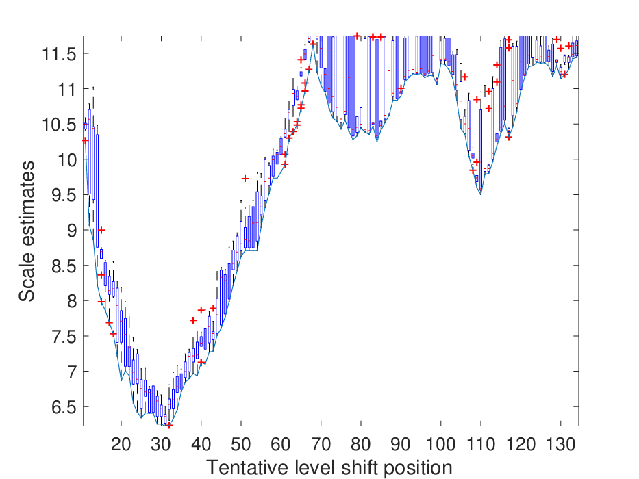
Applying LTS to these contaminated data correctly detects the level shift at time 100, as seen in Figure 15 with the objective function and its local refinement (similar to Figure 5). The resulting double wedge plot in the top panel of Figure 16 actually reveals both level shifts. Interestingly, the LTS fit in the lower panel of Figure 16 flags the first 30 points as a stretch of outliers.
In the next step we undo the level shift that was found, by subtracting from in all . To this modified time series we again apply LTS, which now correctly detects the level shift at time 31 as seen in Figure 17. The resulting double wedge plot in Figure 18 now shows only this level shift (since the other one has been removed). The final fit no longer shows any outliers. If we undo also the second level shift and run LTS again, no more level shifts are found.
 |
 |
| (a) | (b) |
We also ran examples where the level shifts had roughly the same size and with more than two level shifts, with similar results.