Status of Complex Langevin

After the method was proposed in 1983 by G. Parisi [19] and independently by J. Klauder [20], the 1980s and 1990s saw many studies, sometimes showing success, but sometimes the method failed to reach convergence and sometimes, even worse, it converged, but to an incorrect limit [21, 22] not satisfying Eq.(1).

This negative finding almost killed interest in the method, but the interest was rekindled by a paper J. Berges and I.-O. Stamatescu [23], which showed some success in computing correlation functions of a quantum field theory at real time.

The presence or absence of boundary terms at $\infty$ under integration by parts will depend on the decay of the distribution of $|\vec{K}{\cal O}P|$ as we move towards $\infty$.

In some toy models we are in luck: the equilibrium distribution is confined in a strip, i.e. at least the imaginary part remains bounded. An example [38] is

$${\cal M}=\mathbb{R},\;{\cal M}_{c}=\mathbb{C},\;S=\frac{1}{2}(1+iB)x^{2}+\frac{1}{4}x^{4}\,.$$

(27)

In this case the equilibrium distribution is confined in a strip provided $B<\sqrt{3}$ and the CL simulation gives correct results.

The plot Fig.1, taken from [38] shows the emergence of skirts as $B$ is increasing, crossing the critical value $\sqrt{3}$; it displays histograms of the partially integrated equilibrium density

$$P_{y}(y)\equiv\int P(x,y)dx\,.$$

(28)

The tails behave like $O((x^{2}+y^{2})^{-3})$ and the results deteriorate as $B$ becomes $>\sqrt{3}$.

This section follows largely our paper [40]. If $\rho$ has zeroes in ${\cal M}_{c}$, $\vec{K}$ has poles there. The evolution $\dot{{\cal O}}=L_{c}{\cal O}$ then generically produces essential singularities at these locations.

In equilibrium poles may be

• •

  outside of the distribution: in this case they are harmless

• •

  at the edge of the distribution: the behavior of $|\vec{K}P|$ determines success or failure

• •

  inside the distribution: success of failure depend on the behavior of $|\vec{K}P|$ and ergodicity

Nagata, Nishimura, Shimasaki [39] propose to monitor skirts of $|\vec{K}P|$ at poles as well as at $\infty$. This is an excellent idea, allowing to analyze both kinds of boundary terms the same way.

We study these issues first in a simple one-pole model given by

$$\rho(x)=(x-iy_{p})^{n_{p}}\exp(-\beta x^{2})\,,$$

(29)

choosing $y_{p}=1$ for concreteness. The situation is illustrated in Fig.2: For $\beta<2n_{p}/y_{p}^{2}$ we have $P(x,y)>0$ for $0<y<y_{p}$ and the pole is on the edge of the equilibrium distribution, whereas for $\beta>2n_{p}/y_{p}^{2}$, $P(x,y)>0$ if and only if $0<y<y_{-}$ and the pole is outside the equilibrium distribution; the upper strip is transient.

This behavior can be understood by looking at the “classical” flow diagrams, see fig. 3 and it can be shown rigorously to be as stated [38, 40].

Fig 4 shows some results of CL simulations for $n_{p}=1$ and $\beta=0.8\;,1.6\;,3.2$ and $4.8$ as well as for $n_{p}=2$ and $\beta=1.6\;,3.2$. In both cases the results improve dramatically with increasing $\beta$; for $n_{p}=1$, $\beta=1$ is already large enough, whereas for $n_{p}=2$ CL results are still quite wrong for this $\beta$. The reason for this difference is that $n_{p}$ is multiplying the pole term in the drift and so with increasing $n_{p}$ the pull towards the pole becomes stronger.

Let us now focus on $n_{p}=2$. For $\beta=3.2$ and $4.8$ there is excellent agreement between simulation results and the exact values. For $\beta=4.8$ (pole outside the distribution) this is to be expected, but it may be surprising that for $\beta=3.2$, with the pole on the edge, CL still produces excellent results, unlike the situation for $\beta=1.6$. The reason is the different behavior of the distribution near the poles for $\beta=3.2$ compared to $\beta=1.6$, as shown in Fig.5. For $\beta=1.6$ there is a considerable boundary term, whereas for $\beta=3.2$ such a boundary term is either absent or invisibly small.

To see what happens with poles inside the distribution, we turn to another simple model: the one-link U(1) model given by:

$$\rho(x)=D(x)\exp[\beta\cos(x)];\;\;\kappa=2,\;\mu=1\,,$$

(30)

where

$$D(x)\equiv\left[1+\kappa\cos(x-i\mu)\right]^{n_{p}}$$

(31)

is a mockup of the fermion determinant in a lattice model. We show the classical flow portrait for $\beta=0.3$ and three values of $n_{p}$ in Eq.(6). Note that besides the attractive fixed point of the flow at ${\rm Im}\,z=0$ there is a secondary one at ${\rm Im}\,z=\pm\pi$.

The equilibrium distributions for the same cases are shown in Fig.7. For $n_{p}=1,2$ they show two almost separated regions defined by

$$G_{\pm}\equiv\{z\in\mathbb{C}|\,{\rm sgn}\,{\rm Re}\,D(z)=\pm 1\}\,$$

(32)

visible as the ‘head’ and ‘ears’, respectively. For $n_{p}=4$ we only see one region contained in $G_{+}$.

It can be seen that the process tends to avoid the poles, creating bottlenecks there. But it does not produce correct results (see [40]). The reason will be discussed in the next section, where we find that the CL processes restricted to $G_{+}$ or $G_{-}$ actually simulate correctly a different complex measure.

It is also interesting to study the effect of $\beta$ here as well. We compare the results of simulations for $\beta=0.3$ and $\beta=5$ with the exact results in Fig.8 and see the failure of the simulation for $\beta=0.3$, whereas for $\beta=5$ there is perfect agreement, even though in both cases the drift has a pole in the same place. This of course due to the fact that the large value of $\beta$ makes the attraction of the fixed point at $x=0$ very strong.

Consider a special case of the real one-pole model:

$$\rho=x^{4}\exp\left(-\frac{x^{2}}{2\sigma}\right)\,;\quad K=-\frac{x}{\sigma}+\frac{4}{x}\,.$$

(33)

The Fokker-Planck Hamiltonian related to this model (see Section 1.1) is

$$H_{FP}=-\frac{d^{2}}{dx^{2}}+\frac{2}{x^{2}}+\frac{x^{2}}{2\sigma}-\frac{5}{2\sigma}\,;$$

(34)

$H_{FP}$ has two ground states

$$\Omega_{\pm}\propto\theta(\pm x)x^{2}\exp\left(-\frac{x^{2}}{4\sigma}\right)\,.$$

(35)

Corresponding to these ground states are two equilibrium probability densities:

$$P_{\pm}(x)\propto\Omega_{\pm}^{2}\propto\theta(\pm x)x^{4}\exp\left(-\frac{x^{2}}{2\sigma}\right)\,.$$

(36)

The pole at the origin is a bottleneck, obstructing the crossing of the real CL process.

Returning now to the one-link U(1) model Eq.(30) (Section 2.1), recall that there the poles are also bottlenecks. We venture a bold generalization:

Poles inside the distribution tend to form bottlenecks!

In the simulation for $n_{p}=1,2$ , the process occasionally manages to cross between the regions $G_{+}$ and $G_{-}$, but this might be entirely due to the nonzero step size. For $n_{p}=4$ no such crossing was observed, even in very long runs (Langevin time 25000).

Restricting the simulation process to $G_{+}$ ($G_{-}$), it turns out that it correctly simulates the integral from one pole to the other along a path $C_{+}(C_{-})$ from one pole two the other contained in $G_{+}$ ($G_{-}$)! $C_{+}$ is the path starting at the pole with negative real part and ending at the one with positive real part, whereas $C_{-}$, using the periodicity of the system starts at the latter pole and moves right, ending at the first pole.

This is shown in Fig.9 for $n_{p}=1$ and in Fig.10 for $n_{p}=2$. So probably for $n_{p}=1,2$ and definitely for $n_{p}\geq 4$ there are two invariant (equilibrium) distributions and the process is nonergodic!

In this simple model one can actually obtain correct results for the original problem by combining the two restricted processes with suitable, not always positive weights, $w_{\pm}$:

$$\langle{\cal O}\rangle\equiv w_{+}\langle{\cal O}\rangle_{+}+w_{-}\langle{\cal O}\rangle_{-}\,,$$

(37)

where $\langle{\cal O}\rangle_{\pm}$ are results of the CL simulation restricted to $G_{\pm}$.

$w_{+}$ and $w_{-}$ are easily determined: they are

$$w_{\pm}=\frac{Z_{\pm}}{Z_{+}+Z_{-}}\,,$$

(38)

with

$$Z_{\pm}=\int_{C_{\pm}}\rho(z)dz\,,$$

(39)

For our parameter set $\beta=0.3,\kappa=2,\mu=1$ the weights are:

$n_{p}=1:$ $w_{+}=1.09551,\;w_{-}=-0.09551$,

$n_{p}=2:$ $w_{+}=0.97267,\;w_{-}=0.02733$,

$n_{p}=4:$ $w_{+}=0.99699,\;w_{-}=0.00301$.

The point to take home from this discussion is: absence of boundary terms, i.e. sufficiently fast vanishing of the distribution approaching a pole is necessary for correctness. It is not, however, sufficient, because nonergodicity may mean that a restriction of the desired complex measure is being simulated.

Gauge cooling [42] is a necessary (not always sufficient) procedure for obtaining stable results from CL simulations of lattice gauge theories. It starts with the observation that under complexification of the configuration space of a lattice gauge theory the group of gauge transformations gets complexified as well.

Let’s be concrete and focus on lattice QCD. After integrating out the fermions the configuration space is ${\cal M}\equiv SU(3)^{\times N_{l}}$ which gets complexified to ${\cal M}_{c}\equiv SL(3,\mathbb{C})^{\times N_{l}}$, where $N_{l}\equiv\#$ of links. The gauge group ${\cal G}\equiv SU(3)^{\times N_{s}}$ is complexified to ${\cal G}_{c}\equiv SL(3,\mathbb{C})^{\times N_{s}}$ with $N_{s}\equiv\#$ of sites. The point is that observables ${\cal O}$, analytically continued to ${\cal M}_{c}$ and invariant under ${\cal G}$ are also invariant under the larger, noncompact group ${\cal G}_{c}$. So in the ideal world of mathematics the expectation values of ${\cal O}$ will not change under gauge transformations from ${\cal G}_{c}$; they also would not change if the Langevin process is modified by adding a component tangential to the gauge orbit to the drift $\vec{K}$.

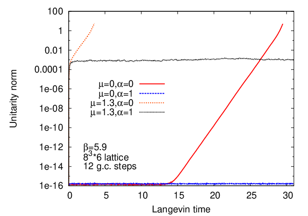
Nevertheless, such a modification of the process is necessary for the following reason: the Langevin process will move, due to buildup of rounding errors, exponentially fast into noncompact directions, far away from the unitary submanifold ${\cal M}$, because the drift $\vec{K}$ produced from a gauge invariant action is gauge covariant and has no component restricting the movement along the gauge orbits of ${\cal G}_{c}$. The link variables thus will soon be very large, whereas the gauge invariant observables composed of them will involve huge cancellations, so that their values will become unreliable. The process will become numerically uncontrolled. This exponential growth is seen in Fig.12, taken from [42] (which will be explained later). So some stabilization of the noncompact directions is definitely necessary.

This can be done either by interspersing some ‘gauge cooling steps’ between ‘dynamical updates’ [42] or by adding a suitable cooling term to the drift, as advocated by [43]. A cooling procedure first requires defining a suitable distance from the unitary submanifold ${\cal M}$, called ‘unitarity norm’; a simple choice is

$$F(\{U\})\equiv\sum_{\vec{x}}{\rm tr}\left[\,{U_{\vec{x}}}^{\dagger}U_{\vec{x}}+({U_{\vec{x}}}^{\dagger})^{-1}{U_{\vec{x}}}^{-1}-2\right]\geq 0\,,$$

(41)

where the sum is over the lattice sites; but of course there are other possibilities (see for instance [44, 39], which are sometimes preferable). $F(\{U\})$ vanishes if and only if all the $U$’s are unitary.

Dynamical updates are defined, using a simple Euler discretization, by

$$U_{\vec{x},\mu}\mapsto\exp\left\{-\sum_{a}i\lambda_{a}(\epsilon K_{a,\vec{x},\mu}+\sqrt{\epsilon}\eta_{a,\vec{x},\mu})\right\}U_{\vec{x},\mu}\,,$$

(42)

where the $\lambda_{a}\,,a=1,\ldots,8$ are the Gell-Mann matrices forming a basis of the Lie algebra of $SU(3)$ and the drift is given by

$$K_{a,\vec{x},\mu}=D_{a,\vec{x},\mu}S$$

(43)

with the derivation $D$ acting on a function $f$ as

$$D_{a,x,\mu}f(\{U\})=\lim_{\delta\to 0}\frac{1}{\delta}\left[f(\{U(\delta)\})-f(\{U\})\right]\,,$$

(44)

where $\{U(\delta)\}$ means the variable $U_{x,\mu}$ has been replaced by $\exp(i\delta\lambda_{a})U_{x,\mu}$ with all other variables unchanged. We define a ‘gauge gradient’ of the unitarity norm by

$$G_{a,\vec{x}}\equiv D_{a,\vec{x}}F=2{\rm tr}\lambda_{a}\left[U_{\vec{x},\mu}U^{\dagger}_{\vec{x},\mu}-U_{\vec{x}-\hat{\mu},\mu}^{\dagger}U_{\vec{x}-\hat{\mu},\mu}\right]+2{\rm tr}\lambda_{a}\left[-(U_{\vec{x},\mu}^{\dagger})^{-1}U_{\vec{x},\mu}^{-1}+(U_{\vec{x}-\hat{\mu},\mu}^{\dagger})^{-1}U_{\vec{x}-\hat{\mu},\mu}^{-1}\right]\,.$$

(45)

The gauge cooling updates of the configuration are then given by

	$\displaystyle U_{x,\hat{\mu}}$	$\displaystyle\mapsto\exp\left(-\sum_{a}\tilde{\alpha}\lambda_{a}G_{a,x}\right)U_{x,\hat{\mu}}\,,$
	$\displaystyle U_{x-\hat{\mu},\mu}$	$\displaystyle\mapsto U_{x-\hat{\mu},\mu}\exp\left(\sum_{a}\tilde{\alpha}\lambda_{a}G_{a,x}\right),$		(46)

where $\tilde{\alpha}=\epsilon\alpha$; $\alpha$ determines the strength of the GC force, whereas $\epsilon$ is a discretization parameter as in Eq.(42). Note that even if $\tilde{\alpha}$ is not small, Eq.(46) is still a gauge transformation; it just might not be optimal for reducing $F$.

Gauge cooling first was shown to work in simple Polyakov loop model, given by a 1D lattice consisting of $N$ links with periodic boundary conditions. [42] Analytically this model reduces to a trivial one-link integral, but it is a useful laboratory.

$$-S=\beta_{1}{\rm tr}U_{1}\ldots U_{N_{t}}+\beta_{2}{\rm tr}U^{-1}_{N}\ldots U^{-1}_{1}\,,$$

(47)

with $\beta_{1,2}$ complex. Simulating this model by using ‘uncooled’ CL for the $N$ links, one discovers that already for $N=16$ one fails to reproduce the correct results. Adding sufficient gauge cooling, however, correct results are obtained.

A more interesting application of GC is the study of the so-called heavy-dense QCD (HDQCD) model, which is obtained by dropping all spatial links from the Wilson fermion action. The plot Fig.12 is from a study of this model [42].

This model had been studied in [45] by reweighting, which is an exact procedure, but unfortunately limited to small lattices; here, however, those results serve as a standard to judge the correctness of CL simulations. In Fig.13 we show a comparison of the reweighted results with those of CL with GC on a $6^{4}$ lattice, taken from [42]. It is seen clearly that for $\beta\geq 5.7$ there is excellent agreement, whereas for $\beta\leq 5.6$ there are considerable deviations.

A natural explanation is that these deviations are due to poles in the drift at the zeroes of the determinant, leading to boundary terms or nonergodicity; just as in the toy models discussed before, increasing $\beta$ makes the process stay away from those dangerous places.

For full QCD there are also some results, some good, some not so good:

In an exploratory study for $\beta=5.9$ on a small ($4^{4}$) lattice Aarts et al [46] used the expansion in the spatial hopping parameter $\kappa_{s}$ for Wilson fermions, truncated at rather high order (up 50) to see convergence; the hopping parameters $\kappa_{s}=\kappa$ were chosen to be 0.12. Agreement of CL for the truncated expansion with CL for the full model supports correctness for this rather large value of $\beta$.

Sexty [41] and later Aarts et al [40] produced results for staggered quarks on lattices up to size $12^{3}\times 4$; there are deviations at smaller $\beta$.

A very detailed study by Fodor et al [47] compared CL with GC for QCD with staggered fermions to multi-parameter reweighting results on lattices up to $16^{3}\times 8$ and again found deviations for smaller $\beta$.

Kogut and Sinclair [48, 49] used staggered quarks on lattices up to $16^{4}$ at $\beta=5.6$ and found unphysical results: no clear ‘silver blaze’ phenomenon and in particular wrong results for $\mu=0$, where the results can be checked by comparing with ordinary Monte Carlo simulations. By increasing $\beta$ to 5.7 that last discrepancy disappeared, in accordance with our general observation that larger $\beta$ values improve the situation. Their results show rather large values for the unitarity norms, which gives already reason for suspecting that the results are not correct (see next section).

Finally I should mention the very recent work by Bloch and Schenk [50] which is using a better matrix inversion method (‘selected inversion’) for the Dirac operator. This improves greatly the stability of the CL simulations, but brings out the deviations for smaller $\beta$ even more clearly.

So this suggests that the incorrect results for QCD at smaller $\beta$ are not due to numerical instabilities, but rather to a more fundamental problem of CL, as discussed earlier in this talk.

Some more encouraging results for larger $\beta$ can be found, however, in [51].

We have seen that CL even with gauge cooling has some issues, which are quite likely due to the zeroes of the fermion determinant. Various cures for this problem have been tried: Nagata et al [39] suggest to use different unitarity norms, Bloch et al [52] propose a variation of the GC procedure. In both cases problems at small $\beta$ remain. Bloch [53] suggests reweighting of CL trajectories; while this works well in simple models, on larger lattices one has to expect overlap problems as always with reweighting.

In my view the most promising, though not sufficiently understood cure is the so-called dynamical stabilization proposed by F. Attanasio and B. Jäger [54, 55, 56]. The following plot Fig.14 taken from[57] and showing once more a simulation of HDQCD, gives some indication about what is going on: if we focus on the purple data, showing the evolution of a certain observable under CL with GC, we see that there is some kind of metastability up to $t\approx 70$, with the data fluctuating around the correct average value. Then the process wanders off fluctuating around a different (and incorrect) value.

A similar effect is also seen in the evolution of the unitarity norm: it first fluctuates around a small, but nonzero value, and then (again at $t\approx 70$) drifts off to a much larger value.

Dynamical stabilization is a somewhat ad hoc fix for this: it consists in the addition of a small extra drift $X$ keeping the unitarity norm small:

	$\displaystyle M^{a}_{\vec{x}}[U]$	$\displaystyle=ib^{a}_{\vec{x}}(b^{a}_{\vec{x}})^{3}\,,\quad b^{a}_{\vec{x}}=\sum_{\nu}{\rm tr}[\lambda^{a}U_{\vec{x}\nu}U_{\vec{x}\nu}^{\dagger}]\,,$
	$\displaystyle X^{a}_{\vec{x}\mu}$	$\displaystyle=i\epsilon\alpha_{DS}M^{a}_{\vec{x}}[U]\,.$		(48)

$X$ is invariant under $SU(3)$ but not $SL(3,\mathbb{C})$ gauge transformations. It is small as long as the unitarity norm remains in the right regime of fairly small values, and it is also small in the sense that it appears to go to zero with increasing $\beta$, indicating that it would disappear in the continuum limit, but it unfortunately invalidates the formal argument for correctness. For $\alpha=0$ it is absent, giving sometimes incorrect results as discussed, whereas for $\alpha=\infty$ it restricts the simulation to the unitary submanifold ${\cal M}$ and is also incorrect. But by choosing $\alpha$ judiciously between those extremes, one can obtain good results.

In the picture Fig.14 [57] it is clearly seen that the extra drift makes the previously metastable region stable ($\alpha$ was chosen appropriately). For details I refer to B. Jäger’s contribution. [56].

It seems, however, necessary to gain a better understanding of the observed metastability. A possible interpretation is that, as in the $U(1)$ one-link model analyzed before, that the system crosses a bottleneck into the basin of attraction of another, ‘unphysical’ attractive fixed point. Dynamical stabilization would then be just a device for preventing this crossing.

It is also conceivable that in order to stabilize the process, the unitary part of the gauge fluctuations needs to be restricted as well as the non-unitary one. Further research into these questions is necessary.

• •

  Insuffient decay both at $\infty$ and at poles may lead to boundary terms spoiling correctness of a CL simulation. Therefore ‘skirts’ or ‘tails’ have to be monitored carefully.

• •

  Gauge cooling eliminates some of the ‘skirts’, but there still may be insufficient decay, so monitoring of them is still necessary.

• •

  Poles are harmless if the process stays away from them; monitoring this in QCD is costly, unfortunately.

• •

  The hopping expansion can sometimes avoid poles (see [46]), but it may still hit problems when $\kappa$ approaches the continuum value.

• •

  The best hope to cure the remaining problems seems to be the ‘dynamical stabilization’, but a better understanding why this works seems necessary.

• •

  In the context of the previous point, it seems highly desirable to gain a deeper understanding of the reason for the observed metastability in QCD, and more generally, understand the essentials of the fixed point and pole structure.

References

- (1) L. L. Salcedo, J. Math. Phys. 38 (1997) 1710 [hep-lat/9607044].
- (2) L. L. Salcedo, J. Phys. A 40 (2007) 9399 [arXiv:0706.4359 [hep-lat]].
- (3) L. L. Salcedo, Phys. Rev. D 94 (2016) no.7, 074503 [arXiv:1510.09064 [hep-lat]].
- (4) L. L. Salcedo, these proceedings.
- (5) D. Weingarten, Phys. Rev. Lett. 89 (2002) 240201 [quant-ph/0210195].
- (6) E. Seiler and J. Wosiek, arXiv:1702.06012 [hep-lat].
- (7) E. Seiler and J. Wosiek, these proceedings.
- (8) A. Wrzykowski, B. Ruba and J. Wosiek, these proceedings.
- (9) B. Ruba and J. Wosiek and A. Wrzykowski these proceedings.
- (10) M. Cristoforetti et al. [AuroraScience Collaboration], Phys. Rev. D 86 (2012) 074506 [arXiv:1205.3996 [hep-lat]].
- (11) A. Alexandru, G. Basar, P. F. Bedaque, G. W. Ridgway and N. C. Warrington, JHEP 1605 (2016) 053 [arXiv:1512.08764 [hep-lat]].
- (12) Y. Mori, K. Kashiwa and A. Ohnishi, arXiv:1705.05605 [hep-lat].
- (13) Y. Tanizaki, these proceedings.
- (14) F. di Renzo, these proceedings.
- (15) J. Nishimura, these proceedings.
- (16) S. Tsutsui, these proceedings.
- (17) A. Ohnishi, these proceedings.
- (18) P. Bedaque, these proceedings.
- (19) G. Parisi, Phys. Lett. 131B (1983) 393.
- (20) J. R. Klauder, Acta Phys. Austriaca Suppl. 25 (1983) 251.
- (21) J. Ambjorn, M. Flensburg and C. Peterson, Phys. Lett. 159B (1985) 335.
- (22) J. Ambjorn, M. Flensburg and C. Peterson, Nucl. Phys. B 275 (1986) 375.
- (23) J. Berges and I.-O. Stamatescu, Phys. Rev. Lett. 95 (2005) 202003 [hep-lat/0508030].
- (24) G. Parisi and Y. s. Wu, Sci. Sin. 24 (1981) 483.
- (25) G. G. Batrouni, G. R. Katz, A. S. Kronfeld, G. P. Lepage, B. Svetitsky and K. G. Wilson, Phys. Rev. D 32 (1985) 2736.
- (26) P. H. Damgaard and H. Huffel, Phys. Rept. 152 (1987) 227.
- (27) E. Nelson, Phys. Rev. 150 (1966) 1079.
- (28) E. Seiler, Acta Phys. Austriaca Suppl. 26 (1984) 259.
- (29) H. Nakazato, Prog. Theor. Phys. 77 (1987) 20.
- (30) K. Okano, L. Schülke and B. Zheng, Prog. Theor. Phys. Suppl. 111 (1993) 313.
- (31) H. Nakazato, K. Okano, L. Schulke and Y. Yamanaka, Nucl. Phys. B 346 (1990) 611.
- (32) G. Aarts, E. Seiler and I. O. Stamatescu, Phys. Rev. D 81 (2010) 054508 [arXiv:0912.3360 [hep-lat]].
- (33) G. Aarts, F. A. James, E. Seiler and I. O. Stamatescu, Eur. Phys. J. C 71 (2011) 1756 [arXiv:1101.3270 [hep-lat]].
- (34) G. Aarts, F. A. James, E. Seiler and I. O. Stamatescu, Phys. Lett. B 687 (2010) 154 [arXiv:0912.0617 [hep-lat]].
- (35) J. R. Klauder and W. P. Petersen, J. Stat. Phys. 39 (1985) 53.
- (36) T. Hayata, Y. Hidaka and Y. Tanizaki, Nucl. Phys. B 911 (2016) 94 [arXiv:1511.02437 [hep-lat]].
- (37) L. L. Salcedo, Phys. Rev. D 94 (2016) no.11, 114505 [arXiv:1611.06390 [hep-lat]].
- (38) G. Aarts, P. Giudice and E. Seiler, Annals Phys. 337 (2013) 238 [arXiv:1306.3075 [hep-lat]].
- (39) K. Nagata, J. Nishimura and S. Shimasaki, Phys. Rev. D 94 (2016) no.11, 114515 [arXiv:1606.07627 [hep-lat]].
- (40) G. Aarts, E. Seiler, D. Sexty and I. O. Stamatescu, JHEP 1705 (2017) 044 [arXiv:1701.02322 [hep-lat]].
- (41) D. Sexty, Phys. Lett. B 729 (2014) 108 [arXiv:1307.7748 [hep-lat]].
- (42) E. Seiler, D. Sexty and I. O. Stamatescu, Phys. Lett. B 723 (2013) 213 [arXiv:1211.3709 [hep-lat]].
- (43) K. Nagata, J. Nishimura and S. Shimasaki, JHEP 1607 (2016) 073 [arXiv:1604.07717 [hep-lat]].
- (44) G. Aarts, F. Attanasio, B. Jäger, E. Seiler, D. Sexty and I. O. Stamatescu, PoS LATTICE 2014 (2014) 200 [arXiv:1411.2632 [hep-lat]].
- (45) R. De Pietri, A. Feo, E. Seiler and I. O. Stamatescu, Phys. Rev. D 76 (2007) 114501 [arXiv:0705.3420 [hep-lat]].
- (46) G. Aarts, E. Seiler, D. Sexty and I. O. Stamatescu, Phys. Rev. D 90 (2014) no.11, 114505 [arXiv:1408.3770 [hep-lat]].
- (47) Z. Fodor, S. D. Katz, D. Sexty and C. Török, Phys. Rev. D 92 (2015) no.9, 094516 [arXiv:1508.05260 [hep-lat]].
- (48) D. K. Sinclair and J. B. Kogut, PoS LATTICE 2016 (2016) 026 [arXiv:1611.02312 [hep-lat]].
- (49) D. Sinclair, these proceedings.
- (50) J. Bloch and O. Schenk, these proceedings.
- (51) I. O. Stamatescu, G. Aarts, K. Boguslawski, M. Scherzer, E. Seiler, D. Sexty, these proceedings.
- (52) J. Bloch, J. Mahr and S. Schmalzbauer, PoS LATTICE 2015 (2016) 158 [arXiv:1508.05252 [hep-lat]].
- (53) J. Bloch, Phys. Rev. D 95 (2017) no.5, 054509 [arXiv:1701.00986 [hep-lat]].
- (54) G. Aarts, F. Attanasio, B. Jäger and D. Sexty, Acta Phys. Polon. Supp. 9 (2016) 621 [arXiv:1607.05642 [hep-lat]].
- (55) F. Attanasio and B. Jäger, PoS LATTICE 2016 (2016) 053 [arXiv:1610.09298 [hep-lat]].
- (56) B. Jäger, these proceedings.
- (57) F. Attanasio, Ph.D. thesis, Swansea University 2017.