Counting quadrant walks via Tutte’s invariant method
August 24, 2026Thanks: This project has received funding from the European Research Council (ERC) under the European Union’s Horizon 2020 research and innovation programme under the Grant Agreement No 759702. OB was partially supported by NSF grants DMS-1400859 and DMS-1800681. KR was partially supported by the project MADACA from the Région Centre-Val de Loire.

Olivier Bernardi , Mireille Bousquet-Mélou and Kilian Raschel Address: OB: Brandeis University, Department of Mathematics, 415 South Street, Waltham, MA 02453, USA
MBM: CNRS, LaBRI, Université de Bordeaux, 351 cours de la Libération, 33405 Talence Cedex, France
KR: CNRS, Institut Denis Poisson, Université de Tours et Université d’Orléans, Parc de Grandmont, 37200 Tours, France

Abstract.

In the 1970s, William Tutte developed a clever algebraic approach, based on certain “invariants”, to solve a functional equation that arises in the enumeration of properly colored triangulations. The enumeration of plane lattice walks confined to the first quadrant is governed by similar equations, and has led in the past 20 years to a rich collection of attractive results dealing with the nature (algebraic, D-finite or not) of the associated generating function, depending on the set of allowed steps, taken in $\{-1,0,1\}^{2}$ .

We first adapt Tutte’s approach to prove (or reprove) the algebraicity of all quadrant models known or conjectured to be algebraic. This includes Gessel’s famous model, and the first proof ever found for one model with weighted steps. To be applicable, the method requires the existence of two rational functions called invariant and decoupling function respectively. When they exist, algebraicity follows almost automatically.

Then, we move to a complex analytic viewpoint that has already proved very powerful, leading in particular to integral expressions for the generating function in the non-D-finite cases, as well as to proofs of non-D-finiteness. We develop in this context a weaker notion of invariant. Now all quadrant models have invariants, and for those that have in addition a decoupling function, we obtain integral-free expressions for the generating function, and a proof that this series is D-algebraic (that is, satisfies polynomial differential equations).

Key words and phrases:

Lattice walks, enumeration, differentially algebraic series, conformal mappings

A tribute to William Tutte (1917-2002), on the occasion of his centenary

1. Introduction

We consider 2-dimensional lattice walks confined to the first quadrant $\mathbb{N}^{2}$ of the plane, as illustrated in Figure 1. The enumeration of such quadrant walks has received a lot of attention in the past 20 years, and given rise to many interesting methods and results. Given a set of steps $\mathcal{S}\subset\mathbb{Z}^{2}$ , the main question is to determine the generating function

(1.1)

Q(x,y;t)\equiv Q(x,y)=\sum_{i,j,n\geqslant 0}q(i,j;n)x^{i}y^{j}t^{n},

where $q(i,j;n)$ is the number of $n$ -step quadrant walks from $(0,0)$ to $(i,j)$ , taking their steps in $\mathcal{S}$ . This is one instance of a more general question consisting in counting walks confined to a given cone. This is a natural and versatile problem, rich of many applications in algebraic combinatorics [BM11, CDD+07, GZ92, Gra02, Kra89], queuing theory [AWZ93, CB83, FH84], and of course in enumerative combinatorics via encodings of numerous discrete objects (e.g. permutations, maps…) by lattice walks [Ber07, BGRR18, GWW98, KMSW19, LSW17].

Figure 1. Three models of walks in the quadrant. The generating function

Q(x,y;t)

is algebraic for the first one, but only D-algebraic for the second. For the third one, it is not even D-algebraic.

At the crossroads of several mathematical fields. Most of the recent progress on this topic deals with quadrant walks with small steps (that is, $\mathcal{S}\subset\{-1,0,1\}^{2}$ ). Then there are $79$ inherently different and relevant step sets (also called models) and a lot is known on the associated generating functions $Q(x,y;t)$ . One of the charms of these results is that their proofs involve an attractive variety of mathematical fields. Let us illustrate this by two results:

•

A certain group $\mathcal{G}$ of birational transformations associated with the model plays a crucial role in the nature of $Q(x,y;t)$ . Indeed, this series is D-finite (that is, satisfies three linear differential equations, one in $x$ , one in $y$ , one in $t$ , with polynomial coefficients in $x,y$ and $t$ ) if and only if $\mathcal{G}$ is finite. This happens for 23 of the 79 models. The positive side of this result (D-finite cases) mostly involves algebra on formal power series [BM02, BMM10, Ges86, GZ92, Mis09]. The negative part relies on a detour via complex analysis and a Riemann-Hilbert-Carleman boundary value problem [Ras12, KR12], or, alternatively, on a combination of ingredients coming from probability theory and from the arithmetic properties of G-functions [BRS14]. The complex analytic approach also provides integral expressions for $Q(x,y;t)$ in terms of Weierstrass’ function.
•

Among the 23 models with a D-finite generating function, exactly 4 are in fact algebraic (that is, $Q(x,y;t)$ satisfies a polynomial equation with polynomial coefficients in $x$ , $y$ and $t$ ). For the most mysterious of them, called Gessel’s model (Figure 1, left), a simple conjecture appeared around 2000 for the numbers $q(0,0;n)$ , but resisted many attempts during a decade. A first proof was then found, based on subtle (and heavy) computer algebra [KKZ09]. The algebraicity was only discovered a bit later, using even heavier computer algebra [BK10]. Since then, two other proofs have been given: one is based on complex analysis [BKR17], and the other is, at last, elementary [BM16a].

Classifying solutions of functional equations. Beyond the solution of a whole range of combinatorial problems, the enumeration of quadrant walks is motivated by an intrinsic interest in the class of functional equations that govern the series $Q(x,y;t)\equiv Q(x,y)$ . These equations involve divided differences (or discrete derivatives) in two variables. For instance, for Kreweras’ walks (steps $\nearrow$ , $\leftarrow$ , $\downarrow$ ), there holds:

(1.2)

Q(x,y)=1+txyQ(x,y)+t\,\frac{Q(x,y)-Q(0,y)}{x}+t\,\frac{Q(x,y)-Q(x,0)}{y}.

This equation is almost self-explanatory, each term corresponding to one of the three allowed steps. For instance, the term

t\,\frac{Q(x,y)-Q(0,y)}{x}

counts walks ending with a West step, which can never be added at the end of a walk ending on the $y$ -axis. The variables $x$ and $y$ are sometimes called catalytic. Such equations (sometimes linear as above, sometimes polynomial) occur in many enumeration problems, because divided differences like

\frac{F(x)-F(0)}{x}\qquad\hbox{or}\qquad\frac{F(x)-F(1)}{x-1}

have a natural combinatorial interpretation for any generating function $F(x)$ . Examples can be found in the enumeration of lattice paths [BF02, BMM10, BMP00], maps [Bro65, BT64, CF16, Tut95], permutations [BM11, BM03, BGRR18]… A complete bibliography would include hundreds of references.

Given a class of functional equations, a natural question is to decide if (and where) their solutions fit in a classical hierarchy of power series:

(1.3)

\hbox{ rational }\subset\hbox{ algebraic }\subset\hbox{ D-finite }\subset\hbox{ D-algebraic},

where we say that a series (say $Q(x,y;t)$ in our case) is D-algebraic if it satisfies three polynomial differential equations (one in $x$ , one in $y$ , one in $t$ ). A historical example is Hölder’s proof that the gamma function is hypertranscendental (that is, not D-algebraic), based on the difference equation $\Gamma(x+1)=x\Gamma(x)$ . Later, differential Galois theory was developed (by Picard, Vessiot, then Kolchin) to study algebraic relations between D-finite functions [vdPS03]. This theory was then adapted to $q$ -equations, to difference equations [vdPS97], and also extended to D-algebraic functions [Mal04]. Let us also cite [DHR18] for recent results on the hypertranscendence of solutions of Mahler’s equations.

Returning to equations with divided differences, it is known that those involving only one catalytic variable $x$ (arising for instance when counting walks in a half-plane) have algebraic solutions, and this result is effective [BMJ06]. Algebraicity also follows from a deep theorem in Artin’s approximation theory [Pop86, Swa98]. For quadrant equations like (1.2) (with two catalytic variables $x$ and $y$ ), the classification with respect to the first three steps of the hierarchy (1.3) is now completely understood. One outcome of this paper deals with the final step: D-algebraicity.

Contents of the paper. We introduce two new objects related to quadrant equations, called invariants and decoupling functions. Both are rational functions in $x$ , $y$ and $t$ . Not all models admit invariants or decoupling functions. We show that these objects play a key role in the classification of quadrant walks (see Table 1 for a summary):

•

First, we prove that invariants exist if and only if the group of the model is finite (that is, if and only if $Q(x,y;t)$ is D-finite); this happens for 23 models. In this case, decoupling functions exist if and only if the so-called orbit sum vanishes (Section 4). This holds precisely for the $4$ algebraic models (Figure 2, left).

Figure 2. Left: The four algebraic quadrant models (Kreweras, reversed Kreweras, double Kreweras, Gessel). Right: Four algebraic models with weights [KY15].
•

In those $4$ cases, we combine invariants and decoupling functions to give short and uniform proofs of algebraicity. This includes the shortest proof ever found for Gessel’s famously difficult model, and extends to models with weighted steps [KY15], for which algebraicity was sometimes still conjectural (Sections 3 and 4).
•

The 56 models with an infinite group have no invariant. But we define for them a certain (complex analytic) weak invariant, which is explicit. Then for the $9$ infinite group models that admit decoupling functions, we give a new, integral free expression for $Q(x,y;t)$ (Section 5). This expression implies that $Q(x,y;t)$ is D-algebraic in $x$ , $y$ and $t$ . This is the first time that D-algebraicity is proved for some non-D-finite quadrant models. We compute explicit differential equations in $y$ for $Q(0,y;t)$ (Section 6).
•

The existence of invariants only depends on the step set $\mathcal{S}$ , but the existence of decoupling functions is also sensitive to the starting point: in Section 7, we describe for which points they actually exist. In particular, we show that some quadrant models that have no decoupling function when starting at $(0,0)$ (and are now known to be non-D-algebraic, as discussed below) still admit decoupling functions when starting at other points. Even though we have not worked out the details, we expect them to be D-algebraic for these points.

Figure 3. The nine D-algebraic models having an infinite group.

An extended abstract of this paper, establishing D-algebraicity for these 9 non-D-finite models, first appeared in 2016 in the proceedings of the FPSAC conference (Formal power series and algebraic combinatorics [BBMR16]). Later, Dreyfus, Hardouin, Roques and Singer completed the differential classification of quadrant walks by proving that the remaining $47$ infinite group models are neither D-algebraic in $x$ (nor in $y$ , by symmetry) [DHRS18, DHRS20], nor in $t$ [DH19] (see also the recent preprint [HS20] on walks with weighted steps). Their proofs rely on Galois theory for difference equations. The complete classification of quadrant models with small steps can now be summarized as in Table 1, which emphasizes the key role of invariants and decoupling functions.

	Decoupling function	No decoupling function
Rational invariant	4 models	19 models
( $\Leftrightarrow$ Finite group)	Algebraic [BMM10, BK10]	D-finite [BMM10]
	Uniform proofs in Section 4	and transcendental [BCvH+17]
No rational invariant	9 models	47 models
( $\Leftrightarrow$ Infinite group)	D-algebraic (Theorem 6.1)	Not D-algebraic
	and not D-finite [KR12, BRS14]	[DHRS18, DHRS20, DH19]

Table 1. Algebraic and differential nature of the generating function

Q(x,y;t)

The genesis of invariants. This paper is inspired by a series of nine papers published by Tutte between 1973 and 1984, starting with [Tut73] and ending with [Tut84], and later surveyed in [Tut95], devoted to the following functional equation in two catalytic variables:

(1.4)

G(x,y;t)\equiv G(x,y)=xq(q-1)t^{2}+\frac{xy}{qt}G(1,y)G(x,y)-x^{2}yt\frac{G(x,y)-G(1,y)}{x-1}+x\frac{G(x,y)-G(x,0)}{y}.

This equation appears naturally when counting planar triangulations properly colored in $q$ colors. Tutte worked on it for a decade, and finally established that $G(1,0)$ is D-algebraic in $t$ . One key step in his study was to prove that for certain (infinitely many) values of $q$ , the series $G(x,y)$ is algebraic, using a pair of (non-rational) series that he called invariants [Tut95]. They are replaced in our approach by (rational) invariants and decoupling functions. After an extension of Tutte’s approach to more general map problems [BBM11, BBM17], this is now the third time that his notion of invariants proves useful, and we believe it to have a strong potential in the study of equations with divided differences.

Strictly speaking, adapting Tutte’s ideas to quadrant walks only provides the algebraicity results of Section 4. In terms of techniques, this simply involves algebraic manipulations on formal power series. The D-algebraicity results of Section 6 require however an analytic notion of invariants, which is the topic of Section 5. The analytic framework that we use there was first developed to study stationary distribution of random walks [FIM99], and then adapted to counting problems [Ras12]. In fact, the weak invariant that we introduce coincides with the so-called gluing function that was already a key object in these analytic approaches. Hence the notion of invariants appears as one way to bridge the gap between the algebraic and analytic approaches to quadrant walks.

2. First steps to quadrant walks

In this section we introduce some basic tools and notation for the study of quadrant walks with small steps (see e.g. [BMM10] or [Ras12]).

Let us begin with some standard notation on power series. For a ring $R$ , we denote by $R[t]$ (resp. $R[[t]]$ , $R((t))$ ) the ring of polynomials (resp. formal power series, Laurent series) in $t$ with coefficients in $R$ . If $R$ is a field, then $R(t)$ stands for the field of rational functions in $t$ . This notation is generalized to several variables. For instance, the series $Q(x,y)$ belongs to $\mathbb{Q}[x,y][[t]]$ . The valuation of a series in $R[[t]]\setminus\{0\}$ is the smallest $n$ such that the coefficient of $t^{n}$ is non-zero.

We will often use bars to denote reciprocals (as long as we remain in an algebraic, non-analytic context): $\bar{x}:=1/x$ , $\bar{y}:=1/y$ .

Consider now the generating function of quadrant walks $Q(x,y)$ defined by (1.1), and recall that the set of steps $\mathcal{S}$ is contained in $\{\-1,0,1\}^{2}$ . A simple step-by-step construction of the walks gives the following functional equation:

(2.1)

K(x,y)Q(x,y)=K(x,0)Q(x,0)+K(0,y)Q(0,y)-K(0,0)Q(0,0)-xy,

where

K(x,y)=xy\Bigg(t\sum_{(i,j)\in\mathcal{S}}x^{i}y^{j}-1\Bigg)

is the kernel of the model. It is a polynomial of degree $2$ in $x$ and $y$ , which we often write as

(2.2)

K(x,y)=\widetilde{a}(y)x^{2}+\widetilde{b}(y)x+\widetilde{c}(y)=a(x)y^{2}+b(x)y+c(x).

We shall also denote

K(x,0)Q(x,0)=R(x)\qquad\hbox{and}\qquad K(0,y)Q(0,y)=S(y).

Note that $K(0,0)Q(0,0)=R(0)=S(0)$ , so that the basic functional equation (2.1) reads

(2.3)

K(x,y)Q(x,y)=R(x)+S(y)-R(0)-xy.

Seen as a polynomial in $y$ , the kernel has two roots $Y_{0}$ and $Y_{1}$ , which are Laurent series in $t$ with coefficients in $\mathbb{Q}(x)$ . If the series $Q(x,Y_{i})$ is well defined, setting $y=Y_{i}$ in (2.3) shows that

(2.4)

R(x)+S(Y_{i})=xY_{i}+R(0).

If this holds for $Y_{0}$ and $Y_{1}$ , then

(2.5)

S(Y_{0})-xY_{0}=S(Y_{1})-xY_{1}.

This equation will be crucial in our paper.

We define analogously the roots $X_{0}$ and $X_{1}$ of $K(x,y)=0$ (when solved for $x$ ).

The group of the model, denoted by $\mathcal{G}(\mathcal{S})$ , is the group of birational transformations of ordered pairs $(u,v)$ generated by the following two transformations:

(2.6)

\Phi(u,v)=\left(\frac{\widetilde{c}(v)}{\widetilde{a}(v)}\frac{1}{u},v\right)\qquad\hbox{and }\qquad\Psi(u,v)=\left(u,\frac{c(u)}{a(u)}\frac{1}{v}\right),

where the polynomials $a,\widetilde{a},c$ and $\widetilde{c}$ are the coefficients of $K$ defined by (2.2). The group operation is composition. For instance,

\Psi\circ\Phi(u,v)=\Psi\left(U,v\right)=\left(U,\frac{c(U)}{a(U)}\frac{1}{v}\right),

where $U=\frac{\widetilde{c}(v)}{\widetilde{a}(v)}\frac{1}{u}$ . One easily checks that both transformations $\Phi$ and $\Psi$ are involutions (that is, $\Phi\circ\Phi=\Psi\circ\Psi=\Id$ ). Thus $\mathcal{G}(\mathcal{S})$ is a dihedral group, which, depending on the step set $\mathcal{S}$ , is finite or not.

Let us take for instance $\mathcal{S}=\{\uparrow,\leftarrow,\searrow\}$ , so that $K(x,y)=txy^{2}+ty+tx^{2}-xy$ . Then $\widetilde{a}(y)=t$ , $\widetilde{c}(y)=ty$ , $a(x)=tx$ , $c(x)=tx^{2}$ , and the basic transformations are

\Phi:(u,v)\mapsto(\bar{u}v,v)\qquad\hbox{and}\qquad\Psi:(u,v)\mapsto(u,u\bar{v}),

with $\bar{u}:=1/u$ and $\bar{v}:=1/v$ . They generate a group of order 6:

(u,v){\overset{\Phi}{\longleftrightarrow}}(\bar{u}v,v){\overset{\Psi}{\longleftrightarrow}}(\bar{u}v,\bar{u}){\overset{\Phi}{\longleftrightarrow}}(\bar{v},\bar{u}){\overset{\Psi}{\longleftrightarrow}}(\bar{v},u\bar{v}){\overset{\Phi}{\longleftrightarrow}}(u,u\bar{v}){\overset{\Psi}{\longleftrightarrow}}(u,v).

Returning to the general case, note that $\Phi$ and $\Psi$ never depend on $t$ , although $K$ does. Indeed,

\frac{c(u)}{a(u)}=\frac{\sum_{(i,-1)\in\mathcal{S}}u^{i}}{\sum_{(i,1)\in\mathcal{S}}u^{i}},

and analogously for ${\widetilde{c}(v)}/{\widetilde{a}(v)}$ . One key property of the transformations $\Phi$ and $\Psi$ is that they leave the step polynomial, namely

P(u,v):=\sum_{(i,j)\in\mathcal{S}}u^{i}v^{j},

unchanged. This is readily checked from the definition of $\Phi$ and $\Psi$ . By composition, the same holds for all elements of $\mathcal{G}(\mathcal{S})$ .

This group was first introduced in the probabilistic context of random walks confined to the quadrant [FIM99]. In our applications, we will typically let it act on pairs $(u,v)$ formed of algebraic functions of the variables $x$ , $y$ and $t$ . In particular, note that

\Phi(X_{0},y)=(X_{1},y)\qquad\hbox{and}\qquad\Psi(x,Y_{0})=(x,Y_{1}).

More generally, since $K(x,y)=xy(tP(x,y)-1)$ , every element $(x^{\prime},y^{\prime})$ in the orbit of $(x,Y_{0})$ (or $(X_{0},y)$ ) satisfies $K(x^{\prime},y^{\prime})=0$ .

The above constructions (functional equation, kernel, roots, group…) can be extended in a straightforward fashion to the case of weighted steps. In this context, if the step $(i,j)$ is weighted by $w_{i,j}$ , the weight of a quadrant walk is the product $W$ of the weights of its steps, and this walk contributes $Wx^{k}y^{\ell}t^{n}$ to the generating function $Q(x,y;t)$ if it has $n$ steps and ends at $(k,\ell)$ . In particular, the kernel becomes:

(2.7)

K(x,y)=xy\Bigg(t\sum_{(i,j)\in\mathcal{S}}w_{i,j}x^{i}y^{j}-1\Bigg).

A step set $\mathcal{S}$ is singular if each step $(i,j)\in\mathcal{S}$ satisfies $i+j\geqslant 0$ .

3. A new solution of Gessel’s model

In this section we illustrate the notions of invariants and decoupling functions, and their use in the solution of quadrant models, by solving Gessel’s model. This model, with steps $\rightarrow,\nearrow,\leftarrow,\swarrow$ , appears as the most difficult model with a finite group. Around 2000, Ira Gessel conjectured that the number of $2n$ -step quadrant walks starting and ending at $(0,0)$ was

q(0,0;2n)=16^{n}\,\frac{(1/2)_{n}(5/6)_{n}}{(2)_{n}(5/3)_{n}},

where $(a)_{n}=a(a+1)\cdots(a+n-1)$ is the rising factorial. This conjecture was proved in 2009 by Kauers, Koutschan and Zeilberger [KKZ09]. A year later, by a computer algebra tour de force, Bostan and Kauers [BK10] proved that the three-variate series $Q(x,y;t)$ is not only D-finite, but even algebraic. Two other, more “human”, proofs have then been given [BKR17, BM16a]. Here, we give yet another proof based on Tutte’s idea of invariants.

The basic functional equation (2.3) holds with $K(x,y)=t(y+x^{2}y+x^{2}y^{2}+1)-xy$ , $R(x)=tQ(x,0)$ , and $S(y)=t(1+y)Q(0,y)$ .

It follows from $K(x,Y_{0})=K(x,Y_{1})=0$ that

(3.1)

J(Y_{0})=J(Y_{1}),\qquad\hbox{ with }\qquad J(y)=\frac{y}{t(1+y)^{2}}+t\bar{y}(1+y)^{2}.

In Tutte’s terminology, $J(y)$ is a (rational) $y$ -invariant. Note that checking that $J(Y_{0})=J(Y_{1})$ from the identities $K(x,Y_{0})=K(x,Y_{1})=0$ is straightforward. We explain in the next section (Theorem 4.6) how $J(y)$ can be constructed.

We now introduce a new variable $u$ that replaces $x$ , and grants interesting properties to the series $Y_{i}(x)$ once they are expressed in terms of $u$ .

Lemma 3.1.

Let $X=t+t^{2}(u+\bar{u})$ , where $u$ is a new variable and $\bar{u}$ stands for $1/u$ . We slightly abuse notation by denoting $Y_{0}$ and $Y_{1}$ the roots of $K(X,y)$ . Then $Y_{0}$ and $Y_{1}$ are Laurent series in $t$ with coefficients in $\mathbb{Q}(u)$ , satisfying

Y_{0}=\frac{u}{t}+\frac{u^{2}(3+2u^{2})}{1-u^{2}}+O(t),\qquad Y_{1}=\frac{\bar{u}}{t}+\frac{\bar{u}^{2}(3+2\bar{u}^{2})}{1-\bar{u}^{2}}+O(t).

The series $Y_{0}$ and $Y_{1}$ simply differ by the transformation $u\mapsto\bar{u}$ . For $i\in\{0,1\}$ , the series $Q(X,Y_{i})$ and $Q(0,Y_{i})$ are well defined as series in $t$ (with coefficients in $\mathbb{Q}(u)$ ).

Proof.

The expansions of the $Y_{i}$ near $t=0$ are found either by solving explicitly $K(X,Y_{i})=0$ , or using Newton’s polygon method [Abh90]. To prove the second point, let us write

Q(x,y)=\sum_{\begin{subarray}{c}a+b\geqslant c+d\\ a\geqslant c\end{subarray}}{\widehat{q}}(a,b,c,d)x^{a+b-c-d}y^{a-c}t^{a+b+c+d},

where ${\widehat{q}}(a,b,c,d)$ is the number of quadrant walks consisting of $a$ North-East steps, $b$ East steps, $c$ South-West steps and $d$ West steps. Given that $X$ and $Y_{i}$ are series in $t$ with respective valuation $\alpha=1$ and $\gamma=-1$ , the valuation of the summand associated with the 4-tuple $(a,b,c,d)$ in $Q(X,Y_{i})$ is

v(a,b,c,d)=\alpha(a+b-c-d)+\gamma(a-c)+(a+b+c+d)=a+2b+c.

For $Q(X,Y_{i})$ to be well defined, we want that for any $n\in\mathbb{N}$ , only finitely many 4-tuples $(a,b,c,d)$ satisfy $a+b\geqslant c+d$ , $a\geqslant c$ and $v(a,b,c,d)\leqslant n$ . The above expression for $v$ shows that $a$ , $b$ and $c$ must be bounded (for instance by $n$ ), and the inequality $a+b\geqslant c+d$ bounds $d$ as well. Hence $Q(X,Y_{i})$ is well defined.

This implies that $Q(0,Y_{i})$ is also well defined, as $Q(0,y)$ is just obtained by selecting the 4-tuples such that $a+b=c+d$ . in the expression of $Q(x,y)$ .

Applying now the generalities of Section 2, we conclude from Lemma 3.1 that (2.5) holds:

(3.2)

S(Y_{0})-{X}Y_{0}=S(Y_{1})-{X}Y_{1}.

Moreover, the kernel equation $K(X,Y_{i})=0$ implies that

XY_{0}-XY_{1}=\frac{1}{t(1+Y_{1})}-\frac{1}{t(1+Y_{0})}.

Note that this is not specific to the choice of $X$ of the form $t+t^{2}(u+\bar{u})$ : when $Y_{0}$ and $Y_{1}$ are the roots of $K(x,y)$ , we still have

(3.3)

xY_{0}-xY_{1}=\frac{1}{t(1+Y_{1})}-\frac{1}{t(1+Y_{0})}.

We will later say that $G(y):=-\frac{1}{t(1+y)}$ is a decoupling function for Gessel’s model (see Section 4.2 for a precise definition). We can then rewrite (3.2) as

(3.4)

L(Y_{0})=L(Y_{1}),\qquad\hbox{with }\qquad L(y)=S(y)+\frac{1}{t(1+y)}.

This should be compared to (3.1). In Tutte’s terminology, the series $L(y)$ is, as $J(y)$ , an invariant, but this time it is (most likely) non-rational. The connection between $J(y)$ and $L(y)$ will stem from the following lemma, which states, roughly speaking, that invariants with polynomial coefficients in $y$ are trivial.

Lemma 3.2.

Let $A(y)$ be a Laurent series in $t$ with coefficients in $\mathbb{Q}[y]$ , of the form

A(y)=\sum_{0\leqslant j\leqslant n/2+n_{0}}a(j,n)y^{j}t^{n}

for some $n_{0}\geqslant 0$ . Let $X=t+t^{2}(u+1/u)$ , and define $Y_{0}$ and $Y_{1}$ as in Lemma 3.1. Then the series $A(Y_{0})$ and $A(Y_{1})$ are well defined Laurent series in $t$ , with coefficients in $\mathbb{Q}(u)$ . If they coincide, then $A(y)$ is in fact independent of $y$ .

Proof.

By considering $A(y)-A(0)$ , we can assume that $A(0)=0$ . In this case,

A(y)=\sum_{1\leqslant j\leqslant n/2+n_{0}}a(j,n)y^{j}t^{n}.

Assume that $A(y)$ is not uniformly zero, and let

m=\min_{n,j}\{n-j:a(j,n)\not=0\}

(see Figure 4 for an illustration). The inequalities $1\leqslant j\leqslant n/2+n_{0}$ imply that $m$ is finite, at least equal to $1-2n_{0}$ . Moreover, only finitely many pairs $(j,n)$ satisfy $m=n-j$ and $j\leqslant n/2+n_{0}$ .

Figure 4. The support of the series

A(y)

, shown with dots, and the definition of

m

Since $j\leqslant n/2+n_{0}$ , any series $Y=c/t+O(1)$ can be substituted for $y$ in $A(y)$ , and

A(Y)=t^{m}\left(\sum_{n-j=m}a(j,n)c^{j}\right)+O(t^{m+1}).

Applying this to $Y_{0}=u/t+O(1)$ and $Y_{1}=\bar{u}/t+O(1)$ , and writing that $A(Y_{0})=A(Y_{1})$ , we obtain

P(u):=\sum_{j\geqslant 1}a(j,m+j)u^{j}=\sum_{j\geqslant 1}a(j,m+j)\bar{u}^{j}=P(\bar{u}).

Hence the polynomial $P(u)$ must vanish, which is incompatible with the definition of $m$ .

The series $J$ and $L$ defined by (3.1) and (3.4) do not satisfy the assumptions of the lemma, as their coefficients are rational in $y$ with poles at $y=0,-1$ (for $J$ ) and $y=-1$ (for $L$ ):

(3.5)

J(y)=\frac{y}{t(1+y)^{2}}+t\bar{y}(1+y),\qquad L(y)=S(y)+\frac{1}{t(1+y)},

with $S(y)=t(1+y)Q(0,y)$ . Still, we can construct from them a series $A(y)$ satisfying the assumptions of the lemma. First, we eliminate the simple pole of $J$ at $0$ by considering $(L(y)-L(0))J(y)$ , which still takes the same value at $Y_{0}$ and $Y_{1}$ . The coefficients of this series have a pole of order at most $3$ at $y=-1$ . By subtracting an appropriate series of the form $C_{1}L(y)^{3}+C_{2}L(y)^{2}+C_{3}L(y)$ , where $C_{1},C_{2}$ and $C_{3}$ depend on $t$ but not on $y$ , we obtain a Laurent series in $t$ satisfying the assumptions of the lemma: the polynomiality of the coefficients in $y$ holds by construction, and the fact that in each monomial $y^{j}t^{n}$ , the exponent of $j$ is (roughly) at most half the exponent of $n$ comes from the fact that this holds in $S(y)$ , due to the choice of the step set (a walk ending at $(0,j)$ has at least $2j$ steps). Thus this series must be constant, equal for instance to its value at $y=-1$ . In brief,

(3.6)

(L(y)-L(0))J(y)=C_{3}L(y)^{3}+C_{2}L(y)^{2}+C_{1}L(y)+C_{0}

for some series $C_{0},C_{1},C_{2},C_{3}$ in $\mathbb{Q}((t))$ . Expanding this identity near $y=-1$ determines the series $C_{0}$ , $C_{1}$ , $C_{2}$ , $C_{3}$ in terms of $S$ . Their expressions are given in the following proposition.

Proposition 3.3.

For $J$ and $L$ defined by (3.5), and $S(y)=t(1+y)Q(0,y)$ , Equation (3.6) holds with

C_{3}=-t,\qquad C_{2}=2+tS(0),\qquad C_{1}=-S(0)+2S^{\prime}(-1)-1/t,

and

C_{0}=-2S(0)S^{\prime}(-1)-3S^{\prime}(-1)/t+S^{\prime\prime}(-1)/t.

Replacing in (3.6) the series $J$ , $L$ and $C_{0},\ldots,C_{3}$ by their expressions in terms of $t$ , $y$ and $S$ gives for $S(y)$ a cubic equation, involving $t$ , $y$ , and three auxiliary unknown series in $t$ , namely $A_{1}:=S(0)$ , $A_{2}:=S_{y}(-1)$ , and $A_{3}:=S_{yy}(-1)$ :

(3.7)

{t}^{2}y\left(y+1\right)^{2}S(y)^{3}-ty\left(y+1\right)\left({t}\left(y+1\right)A_{1}+\left(2\,y-1\right)\right)S(y)^{2}\\ +\left(ty\left(y-1\right)\left(y+1\right)A_{1}-2\,ty\left(y+1\right)^{2}A_{2}+{t}^{2}{y}^{4}+4\,{t}^{2}{y}^{3}+6\,{t}^{2}{y}^{2}+4\,{t}^{2}y+{y}^{3}+{t}^{2}-{y}^{2}\right)S(y)\\ +t(y+1)^{2}(2yA_{2}-{t}(y+1)^{2})A_{1}+y(y+1)(3\,y+1)A_{2}-y(y+1)^{2}A_{3}-ty(y+1)^{3}=0.

(The letter $A$ stands for “auxiliary”, and these series $A_{i}$ , which depend on $t$ only, have no direct connection with the series $A(y)$ of Lemma 3.2.) It is not hard to see that this equation defines a unique 4-tuple of power series, with $A_{i}\in{t}\mathbb{Q}[[t]]$ and $S(y)$ in $t\mathbb{Q}[y][[t]]$ .

Equations of the form

\Pol({S(y)},A_{1},\ldots,A_{k},t,y)=0

occur in the enumeration of many combinatorial objects (lattice paths, maps, permutations…). The variable $y$ is often said to be a catalytic variable. Under certain hypotheses (which generally hold for combinatorially founded equations, and essentially say that these equations have a unique solution $({S(y)},A_{1},\ldots,A_{k})$ in the world of power series), the solutions of such equations are always algebraic, and a procedure for finding them is given in [BMJ06].

Applying the procedure of [BMJ06] to the equation obtained just above for Gessel’s walks (Proposition 3.3) shows in particular that $A_{1},A_{2}$ and $A_{3}$ belong to ${t}\mathbb{Q}(Z)$ , where $Z$ is the unique series in $t$ with constant term 1 satisfying $Z^{2}=1+256t^{2}Z^{6}/(Z^{2}+3)^{3}$ . Details on the solution are given in Appendix A.4. Let us mention that, in the other “elementary” solution of this model, one has to solve an analogous equation satisfied by $R(x)$ [BM16a, Sec. 3.4]. Once $S(y)$ (or equivalently $Q(0,y)$ ) is proved to be algebraic, the algebraicity of $Q(x,0)$ , and finally of $Q(x,y)$ , follow using (2.4) and (2.3).

4. Extensions and obstructions: uniform algebraicity proofs

We now formalize and generalize the three main ingredients in the above solution of Gessel’s model: the rational invariant $J(y)$ given by (3.1), the identity (3.3) expressing $xY_{0}-xY_{1}$ as a difference $G(Y_{0})-G(Y_{1})$ , and finally the “invariant lemma” (Lemma 3.2). We discuss the existence of rational invariants $J$ , and of decoupling functions $G$ , for all quadrant models with small steps in Sections 4.1 and 4.2 respectively. In particular, we relate the existence of rational invariants to the finiteness of the group $\mathcal{G}(\mathcal{S})$ . Then, in Sections 4.3 to 4.5, we show that the above solution of Gessel’s model extends, in a uniform fashion, to all quadrant models (possibly weighted) known or conjectured to have an algebraic generating function (see Figure 2). These 8 models are precisely those that have a rational invariant and a decoupling function. For one of them, we need an algebraic variant of the invariant lemma, which is described in Section 4.4.

4.1. Invariants

To begin with, let us observe that for all models $\mathcal{S}$ that we consider, the associated kernel $K(x,y)$ is irreducible in $\mathbb{Q}(t)[x,y]$ . This could be (tediously) checked case by case, but has been proved more generally in [FIM99, Lem. 2.3.2].

Definition 4.1.

Given a quadrant model $\mathcal{S}$ , and the associated kernel $K(x,y)$ , we define an equivalence relation on elements of $\mathbb{Q}(x,y,t)$ as follows:

A(x,y)\equiv B(x,y)\Leftrightarrow A(x,y)-B(x,y)=K(x,y)\frac{N(x,y)}{D(x,y)}

for $N(x,y)$ and $D(x,y)$ in $\mathbb{Q}(t)[x,y]$ such that $D(x,y)$ is not divisible by $K(x,y)$ in $\mathbb{Q}(t)[x,y]$ .

We have the following simple property.

Lemma 4.2.

Let $A(x,y)$ and $B(x,y)$ be two elements of $\mathbb{Q}(x,y,t)$ that do not have a factor $K(x,y)$ in their denominator (once written in an irreducible form). Then the following conditions are equivalent:

•

$A(x,y)$ and $B(x,y)$ are equivalent,
•

$A(x,Y_{0})=B(x,Y_{0})$ ,
•

$A(x,Y_{1})=B(x,Y_{1})$ .

Proof.

The first point implies the second (or the third) by setting $y=Y_{i}$ in the definition of equivalence. The second (or third) point implies the first by writing $A(x,y)-B(x,y)$ in irreducible form, and using the fact that $K(x,y)$ is irreducible.

Definition 4.3.

A quadrant model admits invariants if there exist rational functions $I(x)\in\mathbb{Q}(x,t)$ and $J(y)\in\mathbb{Q}(y,t)$ , not both in $\mathbb{Q}(t)$ , such that $I(x)\equiv J(y)$ . The functions $I(x)$ and $J(y)$ are said to be an $x$ -invariant and a $y$ -invariant for the model, respectively.

Our definition is more restrictive than that of Tutte [Tut95], who was simply requiring $I(x)$ and $J(y)$ to be series in $t$ with rational coefficients in $x$ (or $y$ ).

The existence of (rational) invariants is equivalent to the following (apparently weaker) condition, which is the one we met in Section 3 (see (3.1)).

Lemma 4.4.

Assume that there exists a rational function $J(y)\in\mathbb{Q}(t,y)\setminus\mathbb{Q}(t)$ such that $J(Y_{0})=J(Y_{1})$ when $Y_{0}$ and $Y_{1}$ are the roots of the kernel $K(x,y)$ , solved for $y$ . Then $I(x):=J(Y_{0})=J(Y_{1})$ is a rational function of $x$ , and $(I(x),J(y))$ forms a pair of invariants.

Proof.

We have $I(x)=(J(Y_{0})+J(Y_{1}))/2$ , hence $I(x)$ is a rational function of $x$ and $t$ as any symmetric function of the roots $Y_{0}$ and $Y_{1}$ . The property $I(x)=J(Y_{i})$ then allows us to conclude that $I(x)\equiv J(y)$ , using Lemma 4.2.

Example. In Gessel’s case, $J(y)$ was given by (3.1), and we find

I(x)=\frac{1}{2}\left(J(Y_{0})+J(Y_{1})\right)=-\frac{t}{x^{2}}+\frac{1}{x}+2t+x-tx^{2}.

We can also check that $K(x,y)$ divides $I(x)-J(y)$ . Indeed,

I(x)-J(y)=-\frac{K(x,y)K(\bar{x},y)}{ty(1+y)^{2}}.

The factor $K(\bar{x},y)$ shows that the pair $(I(x),J(y))$ also forms a pair of invariants for the model $\{\rightarrow,\nwarrow,\leftarrow,\searrow\}$ obtained by reflection in a vertical line. $\hfill{\Box}$

We now generalize this observation, by showing that two models differing by a symmetry of the square have (or have not) invariants simultaneously. Since these symmetries are generated by the reflections in the main diagonal and in the vertical axis, it suffices to consider these two cases.

Lemma 4.5.

Take a model $\mathcal{S}$ with kernel $K(x,y)$ and its diagonal reflection $\widetilde{\mathcal{S}}$ , with kernel $\widetilde{K}(x,y)=K(y,x).$ Then $\widetilde{\mathcal{S}}$ admits invariants if and only if $\mathcal{S}$ does, and in this case a possible choice is $\widetilde{I}(x)=J(x)$ and $\widetilde{J}(y)=I(y).$ A similar statement holds for the vertical reflection $\overline{\mathcal{S}}$ , with kernel $\overline{K}(x,y)=x^{2}K(\bar{x},y),$ where $\bar{x}:=1/x$ . A possible choice is then $\overline{I}(x)=I(\bar{x})$ and $\overline{J}(y)=J(y).$

Proof.

The proof is elementary.

We can now tell exactly which models admit invariants. Note that it is easy to decide whether a given pair $(I,J)$ is a pair of invariants: it suffices to check whether $I(x)-J(y)$ has a factor $K(x,y)$ . The following result tells us how to construct such pairs.

Theorem 4.6.

A (possibly weighted) quadrant model $\mathcal{S}$ has rational invariants if and only if the associated group $\mathcal{G}(\mathcal{S})$ defined by (2.6) is finite.

Assume this is the case, and let $H(x,y)$ be a rational function in $\mathbb{Q}(x,y,t)$ . Consider the rational function

H_{\sigma}(x,y):=\sum_{\gamma\in\mathcal{G}(\mathcal{S})}H(\gamma(x,y)).

Then

I(x)=H_{\sigma}(x,Y_{0})\qquad\hbox{and}\qquad J(y)=H_{\sigma}(X_{0},y)

are respectively rational functions in $(t,x)$ and $(t,y)$ , and they form a pair of invariants, as long as they do not both belong to $\mathbb{Q}(t)$ .

Proof.

Assume that the model has invariants $I(x),J(y)$ , with $I(x)\not\in\mathbb{Q}(t)$ . If $(x^{\prime},y^{\prime})$ is any element in the orbit of $(x,Y_{0})$ , then $K(x^{\prime},y^{\prime})=0$ , hence $I(x^{\prime})=J(y^{\prime})$ . But the form of $\Phi$ and $\Psi$ implies by transitivity that $I(x^{\prime})=I(x)$ and $J(y^{\prime})=J(y)$ .

Assume that the group of the model is infinite. Then the orbit of $(x,Y_{0})$ is infinite as well. Indeed, if it were finite, then there would exist $\gamma\in\mathcal{G}(\mathcal{S})$ , different from the identity, such that $\gamma(x,Y_{0})=(x,Y_{0})$ . Denoting $\gamma(x,y)=(r(x,y),s(x,y))$ , where both coordinates $r$ and $s$ are in $\mathbb{Q}(x,y)$ , this would mean in particular that $r(x,y)-x$ vanishes at $y=Y_{0}$ , forcing this rational function to zero, or to have a factor $K(x,y)$ in its numerator. But this is impossible since $r(x,y)$ does not involve the variable $t$ (while $K$ does), hence $r(x,y)=x$ . By the same argument, $s(x,y)=y$ , hence $\gamma$ is the identity, which contradicts our assumption. Hence the orbit of $(x,Y_{0})$ is infinite. This implies that infinitely many series $x^{\prime}$ occur in it (as the first coordinate of a pair), and thus the equation (in $x^{\prime}$ ) $I(x^{\prime})=I(x)$ has infinitely many solutions. This is clearly impossible since we have assumed that $I(x)\not\in\mathbb{Q}(t)$ .

Conversely, take a model with finite group, a rational function $H(x,y)$ in $\mathbb{Q}(x,y,t)$ , and define $H_{\sigma}$ as above. For instance, for a model $\mathcal{S}$ with a vertical symmetry, $\mathcal{G}(\mathcal{S})$ has order 4, and the orbit of $(x,Y_{0})$ reads:

(x,Y_{0}){\overset{\Phi}{\longleftrightarrow}}(\bar{x},Y_{0}){\overset{\Psi}{\longleftrightarrow}}(\bar{x},Y_{1}){\overset{\Phi}{\longleftrightarrow}}(x,Y_{1}).

Thus if we take $H(x,y)=x$ , then $H_{\sigma}(x,y)=2(x+\bar{x})$ and $J(y)=2(X_{0}+X_{1})=-2\frac{\widetilde{b}(y)}{\widetilde{a}(y)}$ .

Returning to a general group, observe that $H_{\sigma}$ takes the same value, by construction, on all elements of the orbit of $(x,y)$ . In particular, $H_{\sigma}(x,Y_{0})=H_{\sigma}(x,Y_{1})$ . Hence the above defined function $I(x)$ is rational in $x$ and $t$ . Analogously, $J(y)$ is rational in $y$ and $t$ . Moreover, $J(Y_{0})$ , being the sum of $H$ over the orbit of $(x,Y_{0})$ , coincides with $I(x)$ , and by Lemma 4.2, $(I,J)$ is a pair of invariants (unless $I$ and $J$ both depend on $t$ only).

For instance, for the reverse Kreweras model $\left\{\rightarrow,\uparrow,\swarrow\right\}$ , and $H(x,y)=x$ , we find $I(x)=J(y)=1/t$ . But taking instead $H(x,y)=1/x$ gives true invariants:

I(x)=\bar{x}+x/t-x^{2},\qquad J(y)=\bar{y}+y/t-y^{2}.

Let us finally prove that, for any (possibly weighted) model, there exists $k\geqslant 1$ such that the function $I^{(k)}(x)$ obtained from the function $H^{(k)}(x,y)=x^{k}$ actually depends on $x$ . Assume this is not the case. Let $\mathcal{G}(\mathcal{S})$ have order $2n$ , and let $x_{0}=x,x_{1},\ldots,x_{n-1}$ be the $n$ distinct series $x^{\prime}$ that occur in the orbit of $(x,Y_{0})$ as the first coordinate of some pair. Then by assumption, $I^{(k)}(x)=2\sum_{i=0}^{n-1}x_{i}^{k}$ is an element of $\mathbb{Q}(t)$ for all $k$ , which shows that all symmetric functions of the $x_{i}$ ’s depend on $t$ only. This implies that each $x_{i}$ is an algebraic function of $t$ only, which is impossible since $x_{0}=x$ .

Since one of the main objectives of this section is to obtain a uniform solution for algebraic quadrant models, we only give explicit invariants for the four algebraic (unweighted) models (see Table 2). The remaining $19$ models with a finite group either have a vertical symmetry (in which case they admit $I(x)=x+\bar{x}$ as $x$ -invariant), or differ from an algebraic model by a symmetry of the square (in which case Lemma 4.5 applies). Invariants for the four weighted models of Figure 2 are given in Table 4.


$I$	$\frac{t}{x^{2}}-\frac{1}{x}-tx$	$tx^{2}-x-\frac{t}{x}$	$\frac{t}{x}-tx-\frac{1+2t}{1+x}$	$x+\frac{1}{x}-tx^{2}-\frac{t}{x^{2}}+2t$
$J$	$\frac{t}{y^{2}}-\frac{1}{y}-ty$	$ty^{2}-y-\frac{t}{y}$	$\frac{t}{y}-ty-\frac{1+2t}{1+y}$	$\frac{y}{t(1+y)^{2}}+t\frac{(1+y)^{2}}{y}$

Table 2. Rational invariants for algebraic unweighted models.


$I$	$-\frac{t^{2}}{x^{2}}+\frac{t}{x}-t^{2}+tx(1+\lambda t)$	$\frac{{t}^{2}}{x^{2}}-\frac{(1+2t)t}{x}-{{(1+3t)t}x}-{\frac{(1+3t)(1+4t)}{x+1}}+{\frac{(1+3t)^{2}}{(x+1)^{2}}}$	see Lemma 4.5
			and the
$J$	$t^{2}y+\frac{1+\lambda t}{y+1}-\left(\frac{1+\lambda t}{y+1}\right)^{2}$	$\frac{{t}^{2}}{y^{2}}-\frac{(1+2t)t}{y}-{{(1+3t)t}y}-{\frac{(1+3t)(1+4t)}{y+1}}+{\frac{(1+3t)^{2}}{(y+1)^{2}}}$	previous model

Table 3. Rational invariants for weighted models.

In Section 5, we introduce a weaker notion of (possibly non-rational) invariants, which guarantees that any non-singular quadrant model now has a weak invariant. One key difference with the algebraic setting of this section is that the new notion is analytic in nature.

4.2. Decoupling functions

We now return to the identity (3.3), which we first formalize into an apparently more demanding condition.

Definition 4.7.

A quadrant model is decoupled if there exist rational functions $F(x)\in\mathbb{Q}(x,t)$ and $G(y)\in\mathbb{Q}(y,t)$ such that $xy\equiv F(x)+G(y)$ . The functions $F(x)$ and $G(y)$ are said to form a decoupling pair for the model.

Again, this is equivalent to a statement involving a single function $G(y)$ , as used in the previous section (see (3.3)).

Lemma 4.8.

Assume that there exists a rational function $G(y)\in\mathbb{Q}(y,t)$ such that

(4.1)

xY_{0}-xY_{1}=G(Y_{0})-G(Y_{1}),

where $Y_{0}$ and $Y_{1}$ are the roots of the kernel $K(x,y)$ , solved for $y$ . Define $F(x):=xY_{0}-G(Y_{0})=xY_{1}-G(Y_{1})$ . Then $F(x)\in\mathbb{Q}(x,t)$ , and $(F(x),G(y))$ is a decoupling pair for the model.

Proof.

We have

(4.2)

F(x)=\frac{1}{2}\left(xY_{0}-G(Y_{0})+xY_{1}-G(Y_{1})\right),

hence $F(x)$ is a rational function of $x$ and $t$ since it is symmetric in $Y_{0}$ and $Y_{1}$ . By Lemma 4.2, the property $F(x)=xY_{i}-G(Y_{i})$ tells us precisely that $F(x)+G(y)\equiv xy$ .

Example. In Gessel’s case, we had $G(y)=-1/(t(1+y))$ (see (3.3)), corresponding to $F(x)=1/t-1/x$ . $\hfill{\Box}$

Remark. By combining (2.5) and (4.1), we see that if both series $Q(x,Y_{i})$ are well defined, then

S(Y_{0})-G(Y_{0})=S(Y_{1})-G(Y_{1}),

with $S(y)=K(0,y)Q(0,y)$ . In Tutte’s terminology, this would make $S-G$ a second “invariant”. But our terminology is more restrictive, as our invariants must be rational.

Now, which of the $79$ quadrant models are decoupled? Not all, at any rate: for any model that has a vertical symmetry, the series $Y_{i}$ are symmetric in $x$ and $1/x$ , and so any expression for $x$ of the form $(G(Y_{0})-G(Y_{1}))/(Y_{0}-Y_{1})$ would be at the same time an expression for $1/x$ .

In the case of a finite group, we give in Theorem 4.11 below a criterion for the existence of a decoupling pair, as well as an explicit pair when the criterion holds. This shows that exactly four of the $23$ finite group models are decoupled (and these are, as one can expect from the algebraicity result of Section 3, those with an algebraic generating function). The four weighted models of Figure 2, right, are also decoupled.

For models with an infinite group, we have first resorted to an experimental approach to construct decoupling functions. Indeed, one can try to prescribe the form of the partial fraction expansion of $G(y)$ : we first set

G(y)=\sum_{i=1}^{d}a_{i}y^{i}+\sum_{i=1}^{m}\sum_{e=1}^{d_{i}}\frac{\alpha_{i,e}}{(y-r_{i})^{e}},

for fixed values of $d$ , $m$ , $d_{1},\ldots,d_{m}$ , with the values $r_{i}$ of the poles and the coefficients $a_{i}$ and $\alpha_{i,e}$ being yet to determine. We then express $(G(Y_{0})-G(Y_{1}))/(Y_{0}-Y_{1})$ as a rational function in $t$ , $x$ , the $r_{i}$ and $\alpha_{i,e}$ , and require that this is equal to $x$ . This gives a system of polynomial equations relating the $a_{i}$ , $\alpha_{i,e}$ and $r_{i}$ . Solving this system tells us whether the model has a decoupled pair for our choice of $d$ , $m$ and the $d_{i}$ .

In this way, we discovered 9 decoupled models among the 56 that have an infinite group. We could then prove that there are no others. The following theorem summarizes our results.

Theorem 4.9.

Among the $79$ quadrant models, exactly $13$ are decoupled: the $4$ models of Figure 2, left, and the $9$ models of Table 5. Moreover, the $4$ weighted models shown on the right of Figure 2 are also decoupled.

The rest of Section 4.2 is devoted to proving the above theorem. Tables 4 and 5 give explicit decoupling pairs, respectively for finite and infinite groups. One can easily check that they satisfy Definition 4.7. The key point is then to prove that there are no other (unweighted) decoupled models. To prove this, we consider separately the finite and infinite group cases.

Model
$F$	$-\frac{1}{x}+\frac{1}{t}$	$\frac{x}{t}-x^{2}$	$\frac{x-t-tx^{2}}{t(1+x)}$	$-\frac{1}{x}+\frac{1}{t}$	$-x-\frac{1}{x}+\frac{1}{t}$	$-x+\frac{1}{x}-\frac{1+3t}{t(1+x)}+\frac{1+4t}{t}$
$G$	$-\frac{1}{y}$	$-\frac{1}{y}$	$-\frac{1}{y}$	$-\frac{1}{t(1+y)}$	$-\frac{1+\lambda t}{t(1+y)}$	$-y+\frac{1}{y}-\frac{1+3t}{t(1+y)}$


$\frac{(1+3t)^{2}}{t^{2}(1+x)^{2}}-\frac{(1+2t)(1+3t)}{t^{2}(1+x)}+\frac{1+2t}{t}-x$	$-x-\frac{1+3t}{t(1+x)}+\frac{1+t}{t}$
$-y^{2}+\frac{y(1+{t})}{t}+\frac{1+3t}{yt}$	$-y-\frac{1}{y}$

Table 4. Decoupling functions for algebraic models (unweighted or weighted).

Model
$F$	$-x^{2}+\frac{x}{t}-1$	$-x^{2}+\frac{x}{t}$	$-\frac{1}{x}+\frac{1}{t}$	$\frac{1}{x^{2}}-\frac{1}{xt}-x+1$	$-\frac{1}{x}+\frac{1}{t}+1$	$\frac{x-t}{t(x+1)}$
$G$	$-\frac{1}{y}$	$-y-\frac{1}{y}$	$-y-\frac{1}{y}$	$-y^{2}+\frac{y}{t}+\frac{1}{y}$	$-\frac{1+t}{t(y+1)}-y$	$-\frac{1}{y}$


$-x^{2}+\frac{x}{t}-1$	$-x-\frac{1}{x}+\frac{1}{t}$	$\frac{(t+1)^{2}}{(x+1)^{2}t^{2}}-\frac{(1+t)(1+2t)}{(x+1)t^{2}}-\frac{1}{x}-x+1+\frac{1}{t}$
$-y-\frac{1}{y}$	$-\frac{1}{y}-y$	$-\frac{1}{y^{2}}+\frac{1}{ty}+\frac{(t+1)y}{t}-y^{2}$

Table 5. Decoupling functions for nine infinite group models.

4.2.1. The finite group case

In this case, we have found a systematic procedure to decide whether there exists a decoupling pair, and to construct one (when it exists). We consider in fact a more general problem, consisting in writing a rational function $H(x,y)$ as $F(x)+G(y)$ when the pair $(x,y)$ cancels the kernel. The above definition of decoupled models deals with the case $H(x,y)=xy$ , but the general case is not harder and allows us to consider starting points other than $(0,0)$ . This is further discussed in Section 7.

As we shall see, decoupling functions exist if and only if a certain rational function, called orbit sum, vanishes. Our approach adapts [FIM99, Thm. 4.2.9 and Thm. 4.2.10] to our context¹¹ 1 In [FIM99], decoupling functions are called particular rational solutions, as indeed they are particular solutions of the functional equation (2.5). In [DHRS18], they are a certain type of telecopers..

Notation. We recall that the group $\mathcal{G}(\mathcal{S})$ is generated by the involutions $\Phi$ and $\Psi$ defined by (2.6). Its elements consist of all alternating products of $\Phi$ and $\Psi$ . We denote $\Theta=\Psi\cdot\Phi$ , and observe that $\Theta^{-1}=\Phi\cdot\Psi$ . Each element $\gamma$ of the group has a sign, depending on the number of generators $\Phi$ and $\Psi$ that it involves: $\sign(\Theta^{k})=1$ , while $\sign(\Phi\cdot\Theta^{k})=-1$ for all $k$ .

For $A(x,y)\in\mathbb{Q}(x,y)$ , and $\omega=\sum_{\gamma\in\mathcal{G}(\mathcal{S})}c_{\gamma}\cdot\gamma$ an element of the group algebra $\mathbb{Q}[\mathcal{G}(\mathcal{S})]$ , we denote

(4.3)

A_{\omega}(x,y):=\sum_{\gamma\in\mathcal{G}(\mathcal{S})}c_{\gamma}\,A(\gamma(x,y)).

This is again a rational function in $x$ and $y$ . Defining $\sigma$ as the sum of all elements of the group $\mathcal{G}(\mathcal{S})$ , we obtain as a special case the notation $H_{\sigma}(x,y):=\sum_{\gamma\in\mathcal{G}(\mathcal{S})}H(\gamma(x,y))$ used in Theorem 4.6.

We now generalize Definition 4.7.

Definition 4.10.

Given a quadrant model $\mathcal{S}$ , and its kernel $K(x,y)$ , a function $H(x,y)\in\mathbb{Q}(x,y)$ is decoupled if there exist $F(x)\in\mathbb{Q}(x,t)$ and $G(y)\in\mathbb{Q}(y,t)$ such that

H(x,y)\equiv F(x)+G(y).

Theorem 4.11.

Let $\mathcal{S}$ be a step set such that the associated group $\mathcal{G}(\mathcal{S})$ is finite of order $2n$ . Then $H\in\mathbb{Q}(x,y)$ is decoupled if and only if $H_{\alpha}(x,y)=0$ , where $\alpha$ is the following alternating sum:

\alpha=\sum_{\gamma\in\mathcal{G}(\mathcal{S})}\sign(\gamma)\gamma.

In this case, one can take $F(x)=H_{\tau}(x,Y_{0})+H_{\tau}(x,Y_{1})$ , where

\tau=-\frac{1}{n}\sum_{i=1}^{n-1}i\,\Theta^{i}.

The corresponding value of $G$ is then $G(y)=H_{\widetilde{\tau}}(X_{0},y)+H_{\widetilde{\tau}}(X_{1},y)+(1-1/(2n))J(y)$ , where $J(y)$ is the invariant defined in Theorem 4.6 and

\widetilde{\tau}=-\frac{1}{n}\sum_{i=1}^{n-1}i\,\Theta^{-i}.

Proof.

Assume that $H$ is decoupled. Then for every pair $(u,v)$ in the orbit of $(x,Y_{0})$ , we have $K(u,v)=0$ , and hence $H(u,v)=F(u)+G(v)$ . Now recall that if $(u^{\prime},v^{\prime})=\Phi(u,v)$ , then $v^{\prime}=v$ (and analogously for the transformation $\Psi$ ). Hence taking the alternating sum of $H(u,v)=F(u)+G(v)$ over the orbit of $(x,Y_{0})$ , we find that $H_{\alpha}(x,Y_{0})=0$ , which implies that $H_{\alpha}(x,y)$ is uniformly zero since $Y_{0}$ depends on $t$ while $x$ and $H$ do not.

Suppose now that $H_{\alpha}=0$ , and define $F(x)$ and $G(y)$ as above. Note that

F(x)=H_{\tau+\tau\Psi}(x,Y_{0})

and

G(Y_{0})=H_{\widetilde{\tau}+\widetilde{\tau}\Phi+(1-1/(2n))\sigma}(x,Y_{0}),

so that

(4.4)

F(x)+G(Y_{0})=H_{\tau+\tau\Psi+\widetilde{\tau}+\widetilde{\tau}\Phi+(1-1/(2n))\sigma}(x,Y_{0}).

But $\Theta^{i}\Psi=\Theta^{i+1}\Phi$ and $\Theta^{-i}=\Theta^{n-i}$ . Hence

	$\displaystyle\tau+\tau\Psi+\widetilde{\tau}+\widetilde{\tau}\Phi$	$\displaystyle=-\frac{1}{n}\sum_{i=1}^{n-1}i\left(\Theta^{i}+\Theta^{i}\Psi+\Theta^{-i}+\Theta^{-i}\Phi\right)$
		$\displaystyle=-\frac{1}{n}\sum_{i=1}^{n-1}i\left(\Theta^{i}+\Theta^{i+1}\Phi+\Theta^{n-i}+\Theta^{n-i}\Phi\right).$

Upon grouping the terms in $\Theta^{j}$ , and those in $\Theta^{j}\Phi$ , we obtain

\displaystyle\tau+\tau\Psi+\widetilde{\tau}+\widetilde{\tau}\Phi+(1-1/(2n))\sigma

\displaystyle=\id-\frac{1}{2n}\alpha,

where $\sigma$ and $\alpha$ are respectively the sum, and the alternating sum, of the elements of $\mathcal{G}(\mathcal{S})$ . Returning to (4.4), and using $H_{\alpha}=0$ , we obtain that $F(x)+G(Y_{0})=H_{\id}(x,Y_{0})=H(x,Y_{0})$ , so that the pair $(F,G)$ indeed decouples $H$ , by Lemma 4.2.

Proof of Theorem 4.9 in the finite group case.

We now apply Theorem 4.11 to $H(x,y)=xy$ and to the $23$ models with a finite group (listed for instance in [BMM10, Sec. 8]). We find indeed that the alternating orbit sum of $H(x,y)$ vanishes in four cases only. Applying to them the procedure of the theorem gives the decoupling functions of Table 4. The procedure applies as well to weighted models. Note that we have sometimes replaced the pair $(F,G)$ of Theorem 4.11 by the decoupling pair $(F+cI,G-cJ)$ , where $(I,J)$ is a pair of invariants, to simplify the expression $G(y)$ .

4.2.2. The infinite group case.

Recall that we have discovered experimentally $9$ decoupled models with an infinite group, shown in Table 5. Of course, it is straightforward to check, in each case, that $F(x)+G(y)-xy$ is divisible by the kernel. Now how can we prove that the remaining $47$ models with an infinite group are not decoupled? Unfortunately, when $\mathcal{G}(\mathcal{S})$ is infinite, we have not found any criterion comparable to Theorem 4.11 that would decide whether the function $H(x,y)=xy$ is decoupled. Our approach involves some case-by-case analysis, and relies on the two following observations. Here, we assume that $(F(x),G(y))$ is a decoupling pair, and denote by $\mathbb{K}$ the algebraic closure of $\mathbb{Q}(t)$ .

•

If $X\in\mathbb{K}$ is a pole of $F(x)$ , and $Y\in\mathbb{K}$ satisfies $K(X,Y)=0$ , then $Y$ is a pole of $G(y)$ . By a symmetric argument, if $X^{\prime}\in\mathbb{K}$ satisfies $K(X^{\prime},Y)=0$ , then $X^{\prime}$ is another pole of $F(x)$ . Since a rational function has only finitely many poles, this procedure must stop or loop at some point. This is formalized in Lemma 4.13.
•

If $u\in\mathbb{C}$ is a root of the polynomial $a(x)=[y^{2}]K(x,y)$ , then either it is a pole of $F(x)$ , or $G(y)/y$ tends to $u$ at infinity (Lemma 4.14).

The idea is then to argue ad absurdum. We choose a root $u$ of $a(x)$ , and prove, thanks to the first observation, that it cannot be a pole of $F$ (because the propagation of poles does not stop for the value $u$ ). We then use the second observation to determine the behavior of $G(y)/y$ at infinity, and derive some contradiction from it. Note that the idea of propagating poles is classical when searching for rational solutions of difference equations (see e.g. [Abr95]), and is also used in the quadrant context in [DHRS18].

In order to formalize the above observations, we first need to introduce a variant of the transformations $\Phi$ and $\Psi$ defined in (2.6).

Definition 4.12.

Let $(X,Y)\in\mathbb{K}^{2}$ satisfy $K(X,Y)=0$ . We define $\phi(X,Y)=(X^{\prime},Y)$ , where $X^{\prime}$ is the other root (if any) of the equation $K(x,Y)=0$ (solved for $x$ ). We define analogously $\psi(X,Y)=(X,Y^{\prime})$ , where $Y^{\prime}$ is the other root of the equation $K(X,y)=0$ , solved for $y$ .

For $X\in\mathbb{K}$ , the equation $K(X,y)=0$ , when solved for $y$ , has at most two solutions $Y$ and $Y^{\prime}$ , which belong to $\mathbb{K}$ as well (we ignore infinite solutions). The $x$ -orbit of $X$ is the set of pairs in $\mathbb{K}^{2}$ that can be obtained from $(X,{Y})$ or $(X,{Y^{\prime}})$ by repeated applications of the transformations $\phi$ and $\psi$ (as long as they are well defined).

We define the $y$ -orbit of an element $Y$ of $\mathbb{K}$ in a similar fashion, starting from the pairs $({X},Y)$ and $({X^{\prime}},Y)$ such that $K(X,Y)=K(X^{\prime},Y)=0$ .

Recall the expansion (2.2) of $K(x,y)$ in powers of $x$ or $y$ , and the definition (2.6) of the transformations $\Phi$ and $\Psi$ . Then $\phi(X,Y)$ is well defined if and only if $\widetilde{a}(Y)\not=0$ . In this case, $\phi(X,Y)$ coincides with $\Phi(X,Y)$ , unless $X=0$ . Note that $X=0$ implies that $\widetilde{c}(Y)=0$ , and then $X^{\prime}=-\widetilde{b}(Y)/\widetilde{a}(Y)$ , while $\Phi(X,Y)$ is undefined. If $\widetilde{d}(Y)=0$ , where $\widetilde{d}(y)=\widetilde{b}(y)^{2}-4\widetilde{a}(y)\widetilde{c}(y)$ , then $X^{\prime}=X$ and the iterated application of $\phi$ and $\psi$ will not produce any new pair. Of course, analogous statements hold for the determination of $\psi(X,Y)$ .

Examples. Consider the (decoupled) model $\mathcal{S}=\{\nearrow,\uparrow,\leftarrow,\downarrow\}$ , and take $X=0$ , which satisfies $a(X)=0$ . Then $K(X,y)=K(0,y)=ty$ , and the equation $K(X,y)=0$ admits only one root, which is $Y=0$ . So we start from the pair $(0,0)$ . But $\widetilde{a}(Y)=tY^{2}=0$ , thus $K(x,Y)=K(x,0)=tx$ , and the $x$ -orbit of $0$ reduces to the pair $(0,0)$ .

Consider now $\mathcal{S}=\{\uparrow,\nwarrow,\downarrow,\searrow,\rightarrow\}$ (which is also decoupled), and let us determine again the $x$ -orbit of $X=0$ , which satisfies $d(X)=0$ . Since $K(X,y)=K(0,y)=ty^{2}$ , we start from the pair $(X,Y)=(0,0)$ . Now $K(x,Y)=K(x,0)=tx(x+1)$ so we add the pair $\phi(0,0)=(-1,0)=(X^{\prime},Y)$ (note that $\Phi(0,0)$ is not well defined). Finally, $a(X^{\prime})=a(-1)=0$ , thus $K(X^{\prime},y)=K(-1,y)=y(1-t)$ admits only the root $0$ . Hence the $x$ -orbit of $0$ consists of $(0,0)$ and $(-1,0)$ . $\hfill{\Box}$

We can now formalize the two observations made above Definition 4.12.

Lemma 4.13.

Let $(F(x),G(y))$ be a decoupling pair for a model $\mathcal{S}$ . If $X\in\mathbb{K}$ is a pole of $F(x)$ , then for each element $(X^{\prime},Y^{\prime})$ in its $x$ -orbit, $X^{\prime}$ is a pole of $F$ and $Y^{\prime}$ is a pole of $G$ . In particular, the $x$ -orbit of $X$ must be finite.

Consequently, if $X\in\mathbb{K}$ has an infinite $x$ -orbit, then it is not a pole of $F(x)$ .

Proof.

Let us denote

(4.5)

F(x)=\frac{M(x)}{D(x)}\penalty\ \textrm{ and }\penalty\ G(y)=\frac{N(y)}{E(y)},

for some coprime polynomials $M(x),D(x)\in\mathbb{C}(t)[x]$ , and some coprime polynomials $N(y),E(y)\in\mathbb{C}(t)[y]$ . Since $(F,G)$ is a decoupling pair, there exists a polynomial $P(x,y)\in\mathbb{C}(t)[x,y]$ such that

F(x)+G(y)-xy=\frac{K(x,y)P(x,y)}{D(x)E(y)},

or equivalently

(4.6)

M(x)E(y)+D(x)N(y)-xyD(x)E(y)=K(x,y)P(x,y).

If $X$ is a pole of $F$ (that is, a root of $D$ ) and $K(X,Y)=0$ , then (4.6) gives $M(X)E(Y)=0$ . Since $M$ and $D$ have no common root, $E(Y)=0$ and $Y$ is a pole of $G(y)$ . Propagating the reasoning along the $x$ -orbit of $X$ proves the first statement of Lemma 4.13. The second statement follows because $F(x)$ has a finite number of poles.

Lemma 4.14.

Let $(F(x),G(y))$ be a decoupling pair for a model $\mathcal{S}$ . Let $u\in\mathbb{C}$ be a root of $a(x):=[y^{2}]K(x,y)$ that is not a pole of $F(x)$ . Then $\lim_{y\to{\infty}}G(y)/y=u$ .

Proof.

We use the notation (4.5), so that (4.6) holds. Let $E_{d}\,y^{d}$ (resp. $N_{\delta}\,y^{\delta}$ ) be the leading monomial of $E(y)$ (resp. $N(y)$ ). Note that $G(y)\sim N_{\delta}/E_{d}\,y^{\delta-d}$ at infinity. Let $p(x)$ be the leading coefficient of $P(x,y)$ in the variable $y$ . Let us examine the leading monomials, and leading coefficients, in both sides of (4.6):

•

if $\delta<1+d$ , we find $-xD(x)E_{d}=a(x)p(x)$ ,
•

if $\delta=1+d$ , we find $D(x)(N_{\delta}-xE_{d})=a(x)p(x)$ ,
•

if $\delta>1+d$ , we find $N_{\delta}D(x)=a(x)p(x)$ .

Assume now that $u\in\mathbb{C}$ is a root of $a(x)$ but not of $D(x)$ . In the first case, we get $u=0=\lim_{y\rightarrow\infty}G(y)/y$ ; in the second case, we get $N_{\delta}-uE_{d}$ so that $\lim_{y\rightarrow\infty}G(y)/y=N_{\delta}/E_{d}=u$ ; the third case is impossible.

We now derive from the above two lemmas three corollaries that will form our toolbox to prove that none of the 47 models that remain under consideration are decoupled. The first corollary builds on the observation that no decoupled model found so far has $a(x)=t(1+x^{2})$ nor $a(x)=t(1+x+x^{2})$ .

Corollary 4.15.

If the polynomial $a(x)$ has two distinct roots $u$ and $u^{\prime}$ , each of them with an infinite $x$ -orbit, then the model is not decoupled.

Proof.

Assume on the contrary that $(F(x),G(y))$ is a decoupling pair. By Lemma 4.13, neither $u$ nor $u^{\prime}$ can be a pole of $F(x)$ . Hence by Lemma 4.14, we would have $G(y)/y\to u$ and $G(y)/y\to u^{\prime}\not=u$ , which is of course impossible.

Corollary 4.16.

Assume that the polynomial $a(x)$ has a root $u$ with infinite $x$ -orbit, and that one of the branches $Y_{i}(x)$ grows as $|x|^{\nu}$ as $x\to-\infty$ (up to a multiplicative constant, and for infinitely many values of $t$ ), where $\nu>0$ and $\nu\not\in\mathbb{N}$ . Then the model is not decoupled.

In the applications of this corollary that follow, the value of $\nu$ will always be $1/2$ .

Proof.

Suppose on the contrary that a decoupling pair $(F(x),G(y))$ exists. We fix $t\in\mathbb{C}$ such that $F(x)$ and $G(y)$ are well defined and $Y_{i}(x)\sim_{x\to-\infty}|x|^{\nu}$ (up to a multiplicative constant). By Lemmas 4.13 and 4.14 we get $G(Y_{i}(x))\sim_{x\to-\infty}uY_{i}(x)$ . Hence using the decoupling identity $F(x)+G(Y_{i}(x))=xY_{i}(x)$ as $x\to-\infty$ , we get $F(x)\sim_{x\to-\infty}-|x|^{1+\nu}$ , which is not a possible asymptotic behavior for a rational function.

Corollary 4.17.

Assume that $a(x)$ has a root $u$ with infinite $x$ -orbit, that $\widetilde{a}(y):=[x^{2}]K(x,y)$ has a root $v$ with infinite $y$ -orbit, and that moreover one of the branches $Y_{i}(x)$ tends to infinity as $x\to+\infty$ (for infinitely many $t\in\mathbb{C}$ ). Then the model is not decoupled.

Proof.

Suppose on the contrary that a decoupling pair $(F(x),G(y))$ exists. The decoupling identity gives $\frac{F(x)}{xY_{i}(x)}+\frac{G(Y_{i}(x))}{xY_{i}(x)}=1$ , but Lemmas 4.13 and 4.14 (and their counterparts obtained by swapping $x$ and $y$ ) imply that, as $x\to+\infty$ ,

\frac{F(x)}{xY_{i}(x)}\sim\frac{v}{Y_{i}(x)},\qquad\frac{G(Y_{i}(x))}{xY_{i}(x)}\sim\frac{u}{x},

which both tend to $0$ . This yields a contradiction.

As suggested by the above three corollaries, it will be crucial, in what follows, to prove that for a given model $\mathcal{S}$ and a given root $u$ of $a(x)$ , the $x$ -orbit of $u$ is infinite. How can one prove this? We start from the (unique) pair $(x_{0},y_{0}):=(u,y_{0})$ such that $K(u,y_{0})=0$ , and iterate $\phi$ and $\psi$ , thus producing a sequence of $x$ -orbit elements:

(4.7)

(x_{0},y_{0}){\overset{\phi}{\longrightarrow}}(x_{1},y_{0}){\overset{\psi}{\longrightarrow}}(x_{1},y_{1}){\overset{\phi}{\longrightarrow}}(x_{2},y_{1}){\overset{\psi}{\longrightarrow}}\cdots

Each $x_{k},y_{k}$ is rational in $t$ , with coefficients in $\mathbb{Q}(u)$ .

In some cases, it is very simple to prove that the above sequence does not stop nor loop, because $(x_{0},y_{0})$ is the only pair $(X,Y)$ of $\mathbb{Q}(u,t)^{2}$ such that $K(X,Y)=0$ and $a(X)d(X)\widetilde{a}(Y)\widetilde{d}(Y)=0$ . As discussed below Definition 4.12, these are the only pairs where the above chain can stop or loop. Consider for instance $\mathcal{S}=\{\uparrow,\nwarrow,\swarrow,\searrow\}$ , with $u=-1$ . This value $u$ is the only root of $a(x)$ . We find that $y_{0}=-2t$ , so that the $x$ -orbit of $u$ is non-empty. The polynomial $\widetilde{a}(y)$ has no root, and the discriminants $d(x)$ and $\widetilde{d}(y)$ do not factor over $\mathbb{Q}(t)$ . Hence the $x$ -orbit of $u=-1$ is infinite. This argument applies to $8$ cases below and can be adapted to models that are symmetric in the first or second diagonal and have exactly two pairs $(X,Y)$ such that $K(X,Y)=0$ and $a(X)d(X)\widetilde{a}(Y)\widetilde{d}(Y)=0$ . This proves infiniteness of the orbit for $7$ other models.

There is also a more tedious method that applies uniformly to all models under consideration, and proves that the sequence (4.7) is infinite (and does not loop) by looking at the expansions at $t=0$ of the rational functions $x_{k}$ and $y_{k}$ . Two cases occur:

•

If the model $\mathcal{S}$ is singular, that is, $c(x)=tx^{2}$ and $\widetilde{c}(y)=ty^{2}$ , then it is easy to see, by induction on $t$ , that $x_{k}$ has valuation $2k$ , while $y_{k}$ has valuation $2k+1$ . Indeed, $x_{0}=u$ is a root of $a(x)$ , and is thus a non-zero element of $\mathbb{C}$ since $a(0)=1$ . Then $y_{0}=-c(u)/b(u)$ has valuation $1$ , because $b(u)$ is a non-zero multiple of $t$ while $c(u)$ is a polynomial in $t$ with constant term $-u\not=0$ . Now, suppose that the assumption holds true for $x_{k}$ and $y_{k}$ . We have

$x_{k+1}=\frac{1}{x_{k}}\frac{\widetilde{c}(y_{k})}{\widetilde{a}(y_{k})}.$

Using $\widetilde{c}(y)=ty^{2}$ and $\widetilde{a}(y)=t(1+O(y))$ , we find that $x_{k+1}$ has valuation $2k+2$ . Then

$y_{k+1}=\frac{1}{y_{k}}\frac{c(x_{k+1})}{a(x_{k+1})},$

and an analogous argument proves that $y_{k+1}$ has valuation $2k+3$ in $t$ .

•

If $\mathcal{S}$ is not singular, the details of the argument depend on the details of the model. Consider for instance $\mathcal{S}=\{\nearrow,\nwarrow,\swarrow,\downarrow\}$ , with $u=i$ . Using again the notation (4.7), we have $x_{0}=i$ , $y_{0}=(1-i)t$ , and pushing the calculations further suggests that $x_{3k}=i+4kit^{2}+O(t^{4})$ . Clearly, this would imply that the $x$ -orbit is infinite. To prove this, we proceed as follows. Let $X_{0}=i+\sum_{n\geqslant 2}a_{n}t^{n}$ be a series in $t$ with complex coefficients, with $a_{2}\not=-4i$ (the reason for this condition will appear later). One of the roots of the equation $K(X_{0},Y)=0$ reads $Y_{0}=(1-i)t+O(t^{3})$ , as can be seen from the equation $Y=\frac{t}{X_{0}}(1+X_{0}+Y^{2}+X_{0}^{2}Y^{2})$ . The coefficients of $Y_{0}$ lie in $\mathbb{Q}[i,a_{2},a_{3},\ldots]$ . We then compute $X_{1},X_{2},X_{3}$ , and $Y_{1},Y_{2},Y_{3}$ such that

(X_{0},Y_{0}){\overset{\phi}{\longrightarrow}}(X_{1},Y_{0}){\overset{\psi}{\longrightarrow}}(X_{1},Y_{1}){\overset{\phi}{\longrightarrow}}(X_{2},Y_{1}){\overset{\psi}{\longrightarrow}}(X_{2},Y_{2}){\overset{\phi}{\longrightarrow}}(X_{3},Y_{2}){\overset{\psi}{\longrightarrow}}(X_{3},Y_{3}).

(In practice, we compute them using the transformations $\Phi$ and $\Psi$ .) We thus obtain:

$\displaystyle X_{1}$	$\displaystyle=\frac{1}{2t^{2}}+O(1),$	$\displaystyle Y_{1}=(1+i)t+O(t^{3}),$
$\displaystyle X_{2}$	$\displaystyle=-i+(4i+a_{2})t^{2}+O(t^{3}),$	$\displaystyle Y_{2}=\frac{1}{2(4i+a_{2})t^{3}}+O(t^{-2}),$
$\displaystyle X_{3}$	$\displaystyle=i+(4i+a_{2})t^{2}+O(t^{3}),$	$\displaystyle Y_{3}=(1-i)t+O(t^{3}).$

The condition $a_{2}\not=-4i$ is required because, while the coefficients of $X_{1},X_{2},X_{3}$ , and $Y_{1},Y_{3}$ lie in $\mathbb{Q}[i,a_{2},a_{3},\ldots]$ , those of $Y_{2}$ lie in $\mathbb{Q}[i,1/(a_{2}+4i),a_{2},a_{3},\ldots]$ . We observe that the pair $(X_{3},Y_{3})$ has the same form as $(X_{0},Y_{0})$ , with $a_{2}$ replaced by $4i+a_{2}$ , and this completes the proof. We say that the $x$ -orbit of $u=i$ has pseudo-period $3$ .

We now apply our toolbox to the proof of Theorem 4.9, in the infinite group case. We distinguish several cases, depending on the value of $a(x)=[x^{2}]K(x,y)$ . A Maple session, available on the authors’ webpages, examines in detail all non-decoupled models.

Case 1: $\boldsymbol{a(x)=t(1+x^{2})}$ .

The polynomial $a(x)$ has two roots, namely $i$ and $-i$ . By Corollary 4.15, it suffices to prove that their $x$ -orbits are infinite to conclude that the model does not decouple. The corresponding $7$ models are labeled 1a in Table 6. One is singular, and for the others, the $x$ -orbit of $u=\pm i$ has pseudo-period ranging from $2$ to $7$ . The same argument applies to the $10$ models labeled 1b in Table 6, for which $\widetilde{a}(y)=t(1+y^{2})$ , upon exchanging the roles of $x$ and $y$ . Again, one of these models is singular, and for the others, the $y$ -orbit of $v=\pm i$ has pseudo-period ranging from $2$ to $7$ . We have thus proved non-decoupling for 17 models with an infinite group.

Case 2: $\boldsymbol{a(x)=t(1+x+x^{2})}$ .

We now apply Corollary 4.15 to the roots $j$ and $1/j$ , with $j=e^{2i\pi/3}$ . This proves non-decoupling for 12 additional models, indicated in Table 6 by 2a and 2b (depending on whether the argument is applied to $a(x)$ or $\widetilde{a}(y)$ ). As before, we find $x$ - and $y$ -orbits with pseudo-periods ranging from $2$ to $7$ , in addition to one singular model.

Case 3: $\boldsymbol{a(x)=t(1+x)}$ .

It can be checked that for every (yet untreated) model such that $a(x)=t(1+x)$ , the $x$ -orbit of $u=-1$ is infinite.

If moreover $\deg(b(x))\leqslant 1$ , then $\deg(c(x))=2$ (because there is at least one step with $x$ -coordinate $+1$ ), and we have, for any non-zero real $t$ ,

Y_{i}(x)=\frac{-b(x)\pm\sqrt{b(x)^{2}-4a(x)c(x)}}{2a(x)}\sim_{x\to-\infty}|x|^{1/2},

up to some multiplicative constant. We then conclude by Corollary 4.16. This takes care of the $7$ models labeled 3.1a in Table 6.

For the four models labeled 3.2a in the table, we can apply instead Corollary 4.17. First, $u=-1$ is a root of $a(x)$ and has an infinite orbit. Then, $\widetilde{a}(y)=t(1+y)$ , and $v=-1$ is a root of $\widetilde{a}(y)$ with an infinite $y$ -orbit. Finally, $b(x)$ has degree 2, and for $t>0$ ,

Y_{1}(x)=\frac{-b(x)-\sqrt{b(x)^{2}-4a(x)c(x)}}{2a(x)}\sim_{x\to\pm\infty}-x.

Let us now exchange the roles of $x$ and $y$ . Then the same argument applies to the model labeled 3.2b: we have $\widetilde{a}(y)=t(1+y)$ and $v=-1$ has an infinite $y$ -orbit, $a(x)=tx$ and $u=0$ has an infinite $x$ -orbit, and finally one of the branches $X_{i}(y)$ diverges at infinity.

As before, we find $x$ - and $y$ -orbits with pseudo-periods ranging from $2$ to $7$ (in addition to two singular models).

Case 4: $\boldsymbol{a(x)=tx}$ .

The argument is similar to the one used in the previous case. This time we apply it with $u=0$ . It can be checked that for each (yet untreated) model of the table such that $a(x)=tx$ , the $x$ -orbit of $0$ is infinite.

For the three non-symmetric such models (labeled 4.1a), $b(x)$ has degree $0$ , the branches $Y_{i}(x)$ grow like $|x|^{1/2}$ at $-\infty$ , and we conclude using Corollary 4.16. For the symmetric one, labeled 4.2a, $b(x)$ has degree $2$ , and we apply Corollary 4.17 instead, with $u=v=0$ .

The pseudo-periods are found to be $7$ or $8$ in these four cases.

Case 5: the last two models.

We are left with the two symmetric “forks”, $\mathcal{S}_{1}=\{\uparrow,\swarrow,\rightarrow,\nearrow\}$ and its reverse $\mathcal{S}_{2}=\{\leftarrow,\swarrow,\downarrow,\nearrow\}$ . Note that when a symmetric model decouples, there exists a decoupling pair of the form $(F(x),F(y))$ .

For $\mathcal{S}_{1}$ we have $a(x)=tx(1+x)$ , and we can check that the $x$ -orbit of $-1$ is infinite, with pseudo-period $4$ (the $x$ -orbit of $0$ is empty). Hence by Lemma 4.14, $G(y)\sim-y$ at infinity. Both branches $Y_{i}$ are finite at infinity, but as ${x\to 0^{+}}$ , one of the branches $Y_{i}$ is equivalent to $x^{-1/2}$ , so that $G(Y_{i}(x))\sim-x^{-1/2}$ . Plugging this into the decoupling identity $F(x)+G(Y_{i}(x))=xY_{i}(x)$ shows that $F(x)\sim x^{-1/2}$ , which is impossible for a rational function.

For $\mathcal{S}_{2}$ we have $a(x)=tx^{2}$ . We can check that the $x$ -orbit of 0 is infinite, again with pseudo-period $4$ , hence by Lemma 4.13 the decoupling function $F(x)$ is finite at $x=0$ . As ${x\to 0}$ , one of the branches $Y_{i}(x)$ is equivalent to $-1/x^{2}$ , hence expanding the decoupling identity $F(x)+G(Y_{i}(x))=xY_{i}(x)$ around $x=0$ gives $G(Y_{i}(x))\sim-1/x$ . However since $Y_{i}(x)$ grows like $-1/x^{2}$ , this is impossible for a rational function.

This concludes the proof of Theorem 4.9.


3.1a	1a	1b	3.2a	dec. dec. dec. 4.1a		1b 3.1a 1a 1a

5 5 3.1a				dec. 4.1a 1b 1a		dec. 4.2a 3.2b

dec. 2a 2a 4.1a				dec. dec. dec. 3.1a		2a 3.1a 1b 1a

1b 1b 3.1a 2a				2a	3.2a 1b 1a	3.1a 2a 2a 2b

2b 3.2a 1b 1b				1b 2a 1a		3.2a 2a 2a

Table 6. The

56

models with an infinite group. Exactly

9

are decoupled. For the others, we give a label that tells which method can be used to prove that it is not decoupled. These labels refer to the numbering in Section 4.2.2. We have put in the same cell models that only differ by a symmetry of the square.

4.3. The invariant lemma

At this stage, we have found $8$ models ( $4$ unweighted, $4$ weighted), which, as Gessel’s model, admit invariants and are decoupled. They are in fact the $8$ algebraic (or conjecturally algebraic) models of Figure 2. In order to prove their algebraicity as we did in Section 3 for Gessel’s model, we still need to adapt the third and last ingredient of Section 3, namely Lemma 3.2. We can do this for $7$ of our $8$ models. The resisting model is the reverse Kreweras model, with steps $\rightarrow,\uparrow,\swarrow$ . We shall circumvent this difficulty in the next subsection.

Lemma 4.18 (The invariant lemma).

Let $\mathcal{S}$ be one of the models of Figure 2, distinct from the reverse Kreweras model. If $\mathcal{S}$ is one of the last two models, let $X=(1+u)(1+\bar{u})t$ , with $\bar{u}=1/u$ . Otherwise, let $X=t+(u+\bar{u})t^{\beta}$ , where $\beta$ is given in Table 7 below. As in Section 3, we slightly abuse notation by denoting $Y_{0}$ and $Y_{1}$ the roots of $K(X,y)$ . Then $Y_{0}$ and $Y_{1}$ can be expanded around $t=0$ as Puiseux series in $t$ with coefficients in $\mathbb{C}(u)$ , starting with

Y_{0}=ut^{\gamma}(1+o(1))\qquad\hbox{and}\qquad Y_{1}=\bar{u}t^{\gamma}(1+o(1)),

where $\gamma$ is given by Table 7. The series $Q(X,Y_{i})$ and $Q(0,Y_{i})$ are well defined as series in $t$ (or $\sqrt{t}$ when $\gamma$ is a half-integer) with coefficients in $\mathbb{Q}(u)$ .

Let $A(y)$ be a Laurent series in $t$ with polynomial coefficients in $y$ , of the form

A(y)=\sum_{0\leqslant j\leqslant\rho n+n_{0}}a(j,n)y^{j}t^{n},

where $a(j,n)\in\mathbb{Q}$ and $n_{0},\penalty\ \rho$ are constants such that $\rho<1/|\gamma|$ if $\gamma<0$ . Then $A(Y_{0})$ and $A(Y_{1})$ are well defined series in $t$ (or $\sqrt{t}$ ) with coefficients in $\mathbb{Q}(u)$ . If they coincide, then $A(y)$ is in fact independent of $y$ .

The proof mimics the proofs of Lemmas 3.1 and 3.2 used in the Gessel case, where we had $\beta=2$ , $\gamma=-1$ and $\rho=1/2$ .

Model
$\beta$	5/2	3/2	2	2	3/2
$\gamma$	$-1/2$	$-1/2$	$-1$	$-1$	$1/2$	$0$	$0$

Table 7. The values

\beta

and

\gamma

occurring in Lemma 4.18.

It now remains, for each of the $7$ models to which the above lemma applies, to construct a series $A(y)$ satisfying the conditions of the lemma, by combining the invariants of Tables 2 and 3 and the decoupling functions of Table 4. Applying Lemma 4.18 gives for each of these $7$ models a polynomial equation of the form

(4.8)

\Pol(Q(0,y),A_{1},\ldots,A_{k},t,y)=0,

where the series $A_{i}$ are derivatives of $Q(0,y)$ with respect to $y$ , evaluated at $y=0$ or $y=-1$ . These equations are made explicit in Appendix A. The next step will be to solve them, using the general procedure of [BMJ06]. This is described in Section 4.5, and detailed in Appendix A, but we delay this description to establish an equation of the same form for the reverse Kreweras model, to which Lemma 4.18 does not apply.

4.4. An alternative to the invariant lemma

The above method fails for the reverse Kreweras model. The reason is that we have no counterpart of Lemma 4.18: there exists no Puiseux series $X$ in $t$ , with coefficients in $\mathbb{C}(u)$ , such that both roots of $K(X,y)=0$ can be substituted for $y$ in $Q(X,y)$ (the proof is elementary, by considering the valuation of $X$ in $t$ ). However, we will now show that this tool is not essential: if instead of using the equations

J(Y_{0})=J(Y_{1})\qquad\hbox{ and }\qquad xY_{0}-xY_{1}=G(Y_{0})-G(Y_{1}),

we stick to their algebraic origin, namely the fact that $I(x)-J(y)$ and $F(x)+G(y)-xy$ are both divisible by the kernel $K(x,y)$ , then we can still complete the proof using an algebraic argument that does not involve substituting $y$ by the series $Y_{i}$ . This substitution-free approach does work in particular for the reverse Kreweras model.

To clarify this, let us first consider Kreweras’ model, with steps $\nearrow,\leftarrow,\downarrow$ , for which the method that we have described in the previous subsections works. The kernel is

K(x,y)=t(x^{2}y^{2}+x+y)-xy,

and the functional equation reads

(4.9)

K(x,y)Q(x,y)=R(x)+S(y)-xy,

with $R(x)=txQ(x,0)=S(x)$ . The invariants and decoupling functions can be taken as

I(x)=\frac{t}{x^{2}}-\frac{1}{x}-tx=J(x)

and

F(x)=-\frac{1}{x}+\frac{1}{2t}=G(x).

The fact that we can take $I=J$ and $F=G$ comes from the $x/y$ -symmetry of the model.

How does the method presented so far work? First, when $x$ is taken to be $t+(u+\bar{u})t^{5/2}$ , both $Y_{0}$ and $Y_{1}$ can be substituted for $y$ in the functional equation, yielding

(4.10)

S(Y_{0})-xY_{0}=S(Y_{1})-xY_{1}.

Then, the decoupling function allows us to rewrite this as

(4.11)

S(Y_{0})-G(Y_{0})=S(Y_{1})-G(Y_{1}).

The invariant $J$ satisfies the same equation as $S-G$ :

J(Y_{0})=J(Y_{1}).

We now form a third series $A(y)$ satisfying this equation, but having no pole at $y=0$ (nor $t=0$ ):

(4.12)

A(y):=t^{2}\big(S(y)-G(y)\big)^{2}-tJ(y).

By the invariant lemma (Lemma 4.18), $A(y)$ must be independent of $y$ .

We now give a substitution-free version of this argument. What plays the role of (4.10) is simply the functional equation (4.9). The decoupling property stems from

G(x)+G(y)=xy-\frac{K(x,y)}{xyt},

and allows us to rewrite the functional equation as

\big(S(x)-G(x)\big)+\big(S(y)-G(y)\big)=K(x,y)\left(Q(x,y)+\frac{1}{xyt}\right).

This is the counterpart of (4.11). We multiply this equation by $\big(S(x)-G(x)\big)-\big(S(y)-G(y)\big)$ , which gives:

\big(S(x)-G(x)\big)^{2}-\big(S(y)-G(y)\big)^{2}=K(x,y)\left(Q(x,y)+\frac{1}{xyt}\right)\big((S(x)-G(x))-(S(y)-G(y))\big).

This should be compared to the equation

J(x)-J(y)=K(x,y)\frac{y-x}{x^{2}y^{2}},

which underlies the invariant property of $J$ . We now derive from the last two equations an equation satisfied by the pole-free series $A(y)$ defined by (4.12):

A(x)-A(y)=K(x,y)C(x,y),

with

C(x,y)=t^{2}\left(Q(x,y)+\frac{1}{xyt}\right)\big(S(x)-G(x)-S(y)+G(y)\big)-t\ \frac{y-x}{x^{2}y^{2}}.

Using the expressions for $G(y)$ and $S(y)$ , we observe that $C(x,y)$ is a formal power series in $t$ with coefficients in $\mathbb{Q}[x,y]$ . This series, multiplied by the polynomial $K(x,y)$ , decouples as $A(x)-A(y)$ . The following lemma shows that this is impossible, unless $C(x,y)=0=A(x)-A(y)$ . Thus we conclude that $A(x)$ is independent of $x$ , which was a consequence of the invariant lemma in our first approach.

Lemma 4.19.

Consider a quadrant model and its kernel $K(x,y)$ . If there are series $A(x),B(y)$ and $C(x,y)$ in $\mathbb{R}[[x,t]]$ , $\mathbb{R}[[y,t]]$ and $\mathbb{R}[[x,y,t]]$ , respectively, such that $A(x)-B(y)=K(x,y)C(x,y)$ , then $A(x)=B(y)\in\mathbb{R}[[t]]$ and $C(x,y)=0$ .

Proof.

We define a total order on monomials $t^{n}x^{i}y^{j}$ , for $(n,i,j)\in\mathbb{N}^{3}$ , by taking the lexicographic order on $(n,i,j)$ . For a series $S$ , we denote by $\min(S)$ the smallest monomial occurring in $S$ . Then $\min K(x,y)=xy$ . Assume $C(x,y)\not=0$ , and let $M$ be its minimal monomial. Then $xyM$ is the minimal monomial of $K(x,y)C(x,y)$ , and should thus occur in $A(x)-B(y)$ , which is impossible.

We now adapt this to the reverse Kreweras model, with steps $\rightarrow,\uparrow,\swarrow$ . The kernel is

K(x,y)=t(1+x^{2}y+xy^{2})-xy,

and the functional equation reads

K(x,y)Q(x,y)=R(x)+S(y)-S(0)-xy

where now $R(x)=tQ(x,0)=S(x)$ . The invariants and decoupling functions can be taken as

I(x)=t{x^{2}}-x-\frac{t}{x}=J(x)

and

F(x)=-\frac{x^{2}}{2}+\frac{x}{2t}-\frac{1}{2x}=G(x).

The decoupling property stems from

G(x)+G(y)=xy-K(x,y)\frac{x+y}{2xyt},

and allows us to rewrite the functional equation as

\left(S(x)-\frac{S(0)}{2}-G(x)\right)+\left(S(y)-\frac{S(0)}{2}-G(y)\right)=K(x,y)\left(Q(x,y)+\frac{x+y}{2xyt}\right).

Once multiplied by $\big(S(x)-G(x)\big)-\big(S(y)-G(y)\big)$ , this reads

(4.13)

\left(S(x)-\frac{S(0)}{2}-G(x)\right)^{2}-\left(S(y)-\frac{S(0)}{2}-G(y)\right)^{2}=\\ K(x,y)\left(Q(x,y)+\frac{x+y}{2xyt}\right)\big((S(x)-G(x))-(S(y)-G(y))\big).

This should be compared to the invariant property

(4.14)

J(x)-J(y)=K(x,y)\frac{x-y}{xy}.

We now cancel poles at $y=0$ (and $t=0$ ) by considering the series

A(y):=4t^{2}\left(S(y)-\frac{S(0)}{2}-G(y)\right)^{2}-J(y)^{2}+2tS(0)J(y).

A linear combination of (4.13) and (4.14) gives

A(x)-A(y)=K(x,y)C(x,y),

with

C(x,y)=4t^{2}\left(Q(x,y)+\frac{x+y}{2xyt}\right)\left(S(x)-G(x)-S(y)+G(y)\right)-\frac{x-y}{xy}\left(J(x)+J(y)-2tS(0)\right).

Using the expressions for $G(y)$ and $S(y)$ , we observe that $C(x,y)$ is a series in $t$ with coefficients in $\mathbb{Q}[x,y]$ . We conclude as in Kreweras’ case that $C(x,y)=0=A(x)-A(y)$ , so that $A(y)$ is independent of $y$ .

By expanding the series $A(y)$ around $y=0$ , we obtain an equation of the form (4.8), as for the $7$ other models of Figure 2:

(4.15)

4t^{2}\left(S(y)-\frac{S(0)}{2}-G(y)\right)^{2}-J(y)^{2}+2tS(0)J(y)={t}^{2}S(0)^{2}+4{t}^{2}S^{\prime}(0)-4\,t.

We have not checked whether this “substitution-free” invariant lemma works for all models of Figure 2.

4.5. Effective solution of algebraic models

At this stage, for each of the eight models of Figure 2, we have obtained an equation of the form

(4.16)

\Pol(Q(0,y),A_{1},\ldots,A_{k},t,y)=0,

where the series $A_{i}$ are derivatives of $Q(0,y)$ with respect to $y$ , evaluated at $y=0$ or $y=-1$ . Their exact forms are given in Appendix A. It remains to apply the general procedure of [BMJ06] to solve them. This is also detailed in the Appendix, and a Maple session supporting the calculations is available on the authors’ webpages. These calculations are of course heavier when the number $k$ in (4.16) is large: the most complicated models turn out to be Gessel’s model and the last weighted model, for which $k=3$ (we recall that this model was only conjectured to be algebraic [KY15]). For the reverse and double Kreweras models, and for the third weighted model, we have $k=2$ ; while for Kreweras’ model and for the first two weighted models we have $k=1$ .

In all cases the solution is (as already claimed) algebraic. In particular, the generating function $Q(0,0)$ of excursions has degree $3$ , $3$ , $4$ , $8$ , $6$ , $3$ , $3$ , $8$ over $\mathbb{Q}(t)$ , if we scan models from left to right in Figure 2. It is also worth noting that the minimal polynomial of $Q(0,0)$ has genus zero (so that the corresponding curve has a rational parametrization), except for the last weighted model, which had never been solved so far:

Q(0,0)=\frac{-1-6t+\sqrt{Z}}{2t^{2}},

where $Z=1+12t+40t^{2}+O(t^{3})$ satisfies a quartic equation of genus $1$ :

27\,{Z}^{4}-18\left(10000\,{t}^{4}+9000\,{t}^{3}+2600\,{t}^{2}+240\,t+1\right){Z}^{2}\\ +8\left(10\,{t}^{2}+6\,t+1\right)\left(102500\,{t}^{4}+73500\,{t}^{3}+14650\,{t}^{2}+510\,t-1\right)Z\\ =\left(10000\,{t}^{4}+9000\,{t}^{3}+2600\,{t}^{2}+240\,t+1\right)^{2}.

5. An analytic invariant method

In this section we move to an analytic world, and consider $Q(x,y)\equiv Q(x,y;t)$ as a function of three complex variables. We will use several important results from the analytic approach of quadrant walks, developed first in a probabilistic framework [FIM99], and then in an enumerative one [Ras12]. For the reader’s convenience, we will recall all relevant statements.

The main result in this section, Theorem 5.7, tells that, for each decoupled model with an infinite group (shown in Table 5), the series $Q(0,y)$ has a rational expression in terms of $t$ , $y$ , and an explicit function $w(y)$ , which will be seen as a weak invariant. So far, only integral expressions, also involving $w(y)$ , were known. We establish some preliminary technical results in Section 5.1, introduce $w(y)$ in Section 5.2, and prove our main theorem in Section 5.3. The readers who are familiar with the analytic approach to quadrant walks will recognize in the weak invariant $w(y)$ the conformal gluing function that is central in this approach. We conclude in Section 5.4 by showing that this analytic approach applies as well to the four decoupled models with a finite group that we solved in an algebraic fashion in the previous section.

5.1. Preliminaries

Observing that the coefficients of $Q(x,y;t)$ satisfy

\left|\sum_{i,j\geqslant 0}q(i,j;n)x^{i}y^{j}\right|\leqslant|\mathcal{S}|^{n}\max(1,|x|^{n})\max(1,|y|^{n}),

we see that $Q(x,y;t)$ is analytic in $\{|t|\max(1,|x|)\max(1,|y|)<1/|\mathcal{S}|\}$ (at least), and that this domain is a neighborhood of the polydisc $\{|x|\leqslant 1,|y|\leqslant 1,|t|<1/|\mathcal{S}|\}$ .

The roots $Y_{0,1}$ of the kernel (now called branches) are

Y_{0,1}(x)=\frac{-b(x)\pm\sqrt{b(x)^{2}-4a(x)c(x)}}{2a(x)},

where $a,b$ and $c$ are defined in (2.2). The discriminant $d(x):=b(x)^{2}-4a(x)c(x)$ has degree three or four, hence there are four branch points $x_{1},\ldots,x_{4}$ (depending on $t$ ), with $x_{4}=\infty$ if $d(x)$ has degree three. We define analogously the branches $X_{0,1}(y)$ and their four branch points $y_{1},\ldots,y_{4}$ . One key difference with the formal framework adopted so far is the following:

In this section, $t$ is a fixed real number in $(0,1/|\mathcal{S}|)$ .

Moreover, we only consider non-singular, unweighted models.

Lemma 5.1 (Properties of the branch points [Ras12, Sec. 3.2]).

The branch points $x_{\ell}$ are real and distinct. Two of them (say $x_{1}$ and $x_{2}$ ) are in the open unit disc, with $x_{1}<x_{2}$ and $x_{2}>0$ . The other two (say $x_{3}$ and $x_{4}$ ) are outside the closed unit disc, with $x_{3}>0$ and $x_{3}<x_{4}$ if $x_{4}>0$ . The discriminant $d(x)$ is negative on $(x_{1},x_{2})$ and $(x_{3},x_{4})$ , where if $x_{4}<0$ , the set $(x_{3},x_{4})$ stands for the union of intervals $(x_{3},\infty)\cup(-\infty,x_{4})$ .

Of course, analogous results hold for the branch points $y_{\ell}$ .

Figure 5 illustrates schematically the two cases $x_{4}>0$ and $x_{4}<0$ .

Figure 5. Plot of

d(x)

for

x

real: the main two possibilities, depending on the sign of

x_{4}

. Note that

x_{1}

may be non-negative, and

x_{4}

may be

+\infty

The branches $Y_{0,1}$ are meromorphic on $\mathbb{C}\setminus([x_{1},x_{2}]\cup[x_{3},x_{4}])$ . On the cuts $[x_{1},x_{2}]$ and $[x_{3},x_{4}]$ , the two branches $Y_{0,1}$ still exist and are complex conjugate (but possibly infinite at $x_{1}=0$ as discussed in the next lemma). At the branch points $x_{i}$ , we have $Y_{0}(x_{i})=Y_{1}(x_{i})$ (when finite), and we denote this value by $Y(x_{i})$ . A key object in our definition of weak invariants is the curve $\mathcal{L}$ (depending on $t$ ) defined by

\mathcal{L}=Y_{0}([x_{1},x_{2}])\cup Y_{1}([x_{1},x_{2}])=\{y\in\mathbb{C}:K(x,y)=0\text{ and }x\in[x_{1},x_{2}]\}.

By construction, it is symmetric with respect to the real axis.

We denote by $\mathcal{G}_{\mathcal{L}}$ the domain delimited by $\mathcal{L}$ and avoiding the real point at $+\infty$ . See Figure 6 for examples.

Figure 6. The curves

\mathcal{L}

for model

{\#3}

of Table 5 (for

t=0.03

0.1

0.2

0.25=1/|\mathcal{S}|

and

0.263185\ldots

as one moves closer to the origin) and for the reverse Kreweras model (second model in Table 4; from right to left,

t=0.2

0.25

0.28

0.3

and

1/3=1/|\mathcal{S}|

). The dashed curve is obtained for a value

t_{c}\geqslant 1/|\mathcal{S}|

, where

\mathcal{L}

stops being smooth, but here we only consider values of

t

less than

1/|\mathcal{S}|

The following lemma is proved in [FIM99] in the probabilistic framework, that is, when $t=1/|\mathcal{S}|$ (see in particular Thm. 5.3.3 and its proof). We show that it holds for all $t\in(0,1/|\mathcal{S}|)$ as well.

Lemma 5.2 (Properties of the curve $\mathcal{L}$ ).

The curve $\mathcal{L}$ is symmetric with respect to the real axis. It intersects this axis at $Y(x_{2})>0$ .

If $\mathcal{L}$ is unbounded, $Y(x_{2})$ is the only intersection point. This occurs if and only if neither $(-1,1)$ nor $(-1,0)$ belong to $\mathcal{S}$ . In this case, $x_{1}=0$ and the only point of $[x_{1},x_{2}]$ where at least one branch $Y_{i}(x)$ is infinite is $x_{1}$ (and then both branches are infinite there).

Otherwise, the curve $\mathcal{L}$ goes through a second real point, namely $Y(x_{1})\leqslant 0$ . The limit case $Y(x_{1})=0$ occurs if and only if neither $(-1,-1)$ nor $(-1,0)$ belong to $\mathcal{S}$ . In this case, $x_{1}=0$ .

Consequently, the point $0$ is either in the domain $\mathcal{G}_{\mathcal{L}}$ or on the curve $\mathcal{L}$ . The domain $\mathcal{G}_{\mathcal{L}}$ also contains the (real) branch points $y_{1}$ and $y_{2}$ , of modulus less than $1$ . The other two branch points, $y_{3}$ and $y_{4}$ , are in the complement of $\mathcal{G}_{\mathcal{L}}\cup\mathcal{L}$ . The domain $\mathcal{G}_{\mathcal{L}}$ coincides with the region denoted $\mathcal{G}Y([x_{1}(t),x_{2}(t)];t)$ in [Ras12, Lem. 2].

Proof.

Since $d(x)<0$ in $(x_{1},x_{2})$ , the curve $\mathcal{L}$ intersects the real axis at two points at most, namely $Y(x_{1})$ and $Y(x_{2})$ . Recall from (2.2) that

a(x)=tx\sum_{(i,1)\in\mathcal{S}}x^{i},\qquad b(x)=tx\sum_{(i,0)\in\mathcal{S}}x^{i}-x\qquad\hbox{while}\qquad c(x)=tx\sum_{(i,-1)\in\mathcal{S}}x^{i}.

We begin with the polynomial $a(x)$ , which is (at most) quadratic. If $a(x)=0$ for some real $x$ , then $d(x)=b(x)^{2}\geqslant 0$ , hence the sign of $a(x)$ is constant on the interval $(x_{1},x_{2})$ . Since $a(x_{2})>0$ (because $x_{2}>0$ , see Lemma 5.1), we also have $a(x_{1})\geqslant 0$ .

Now consider the polynomial $b(x)$ , which is also quadratic at most. We have $b(0)\geqslant 0$ and $b(1)<0$ (by our choice of $t$ ), hence $b(x)$ has one root $x_{b}$ in $[0,1)$ : exactly one, since if $b(x)$ is quadratic, it must have a root larger than $1$ because $t>0$ . Moreover, $d(x_{b})=-4a(x_{b})c(x_{b})\leqslant 0$ , hence $x_{b}\in[x_{1},x_{2}]$ . In fact $x_{b}\in[x_{1},x_{2})$ since $x_{2}$ is positive and thus satisfies $0<4a(x_{2})c(x_{2})=b(x_{2})^{2}$ . Since $x_{b}<x_{2}<1$ , we have $b(x_{2})<0$ hence $Y(x_{2})=-b(x_{2})/(2a(x_{2}))>0$ . Similarly, since $x_{1}\leqslant x_{b}$ , we have $b(x_{1})\geqslant 0$ .

If $a(x_{1})=0$ , the condition $d(x_{1})=0$ implies that $b(x_{1})=0$ as well. Hence $x_{1}$ coincides with $x_{b}$ , which is non-negative; but $a(x_{b})=0$ then forces $x_{b}=0$ . Thus $b(0)=0=a(0)$ , which is equivalent to saying that neither $(-1,0)$ nor $(-1,1)$ belong to $\mathcal{S}$ . It is readily checked that in this case each $Y_{i}(x)$ tends to infinity as $x\rightarrow 0^{+}$ .

Now assume $a(x_{1})>0$ . Then $Y(x_{1})=-b(x_{1})/(2a(x_{1}))\leqslant 0$ . The limit case $Y(x_{1})=0$ occurs when $b(x_{1})=0$ and $c(x_{1})=0$ (since $d(x_{1})=0$ ). Hence $x_{1}$ coincides again with $x_{b}$ , which is non-negative, and the condition $c(x_{b})=0$ forces $x_{b}=0$ . Thus $b(0)=0=c(0)$ , which is equivalent to saying that neither $(-1,0)$ nor $(-1,-1)$ belong to $\mathcal{S}$ . It is readily checked that in this case $Y(0)=0$ indeed.

It follows from the results established so far that the intersection of the domain $\mathcal{G}_{\mathcal{L}}$ with the real axis is $(Y(x_{1}),Y(x_{2}))$ , where by convention $Y(x_{1})=-\infty$ if $\mathcal{L}$ is unbounded. Moreover, either $Y(x_{1})=0$ and thus $0\in\mathcal{L}$ , or $0\in(Y(x_{1}),Y(x_{2}))$ . We now want to prove that $Y(x_{1})<y_{1}<y_{2}<Y(x_{2})<y_{3}$ , and $y_{4}<Y(x_{1})$ if $y_{4}<0$ . Let us begin with $Y(x_{1})<y_{1}$ , assuming $Y(x_{1})$ is finite (otherwise there is nothing to prove). Define $\widetilde{d}(y)$ as the counterpart for the variable $y$ of the discriminant $d(x)$ , that is, $\widetilde{d}(y)=\widetilde{b}(y)^{2}-4\widetilde{a}(y)\widetilde{c}(y).$ We observe that $\widetilde{d}(Y(x_{1}))\geqslant 0$ : otherwise, the roots of $K(x,Y(x_{1}))$ would be complex conjugate or infinite, while one of them is $x=x_{1}$ . Hence $Y(x_{1})$ cannot be in any of the intervals $(y_{1},y_{2})$ or $(y_{3},y_{4})$ . Since it is non-positive, as proved above, it is necessarily less than or equal to $y_{1}$ , and larger than or equal to $y_{4}$ if $y_{4}<0$ .

Similarly, $Y(x_{2})$ cannot be in any of the intervals $(y_{1},y_{2})$ or $(y_{3},y_{4})$ . Since it is positive (as proved above), it is either larger than or equal to $y_{2}$ , or in $(0,y_{1}]$ . It remains to exclude the two cases $0<Y(x_{2})\leqslant y_{1}$ and $0<y_{4}\leqslant Y(x_{2})$ .

If $0<Y(x_{2})\leqslant y_{1}$ then each function $X_{i}$ is continuous on the interval $[Y(x_{2}),y_{1}]$ . Let $X_{i}$ be the branch of $X$ satisfying $X_{i}(Y(x_{2}))=x_{2}>0$ . Since $X_{i}(y_{1})\leqslant 0$ , there exists a real number $y\in(Y(x_{2}),y_{1}]$ , hence necessarily positive, such that $X_{i}(y)=0$ . That is, $K(0,y)=0=\widetilde{c}(y)$ , which is impossible for $y$ positive.

The argument excluding the case $0<y_{4}\leqslant Y(x_{2})$ is similar: in fact, replacing the step set $\mathcal{S}$ by $\overline{\mathcal{S}}:=\{(i,-j):(i,j)\in\mathcal{S}\}$ leaves the $x_{\ell}$ ’s unchanged, replaces the set $\{y_{\ell}:1\leqslant i\leqslant 4\}$ by $\{1/y_{\ell}:1\leqslant i\leqslant 4\}$ , and finally replaces $Y_{i}$ by $1/Y_{i}$ . With these remarks at hand, one realizes that if $0<y_{4}\leqslant Y(x_{2})$ for one model, then $0<Y(x_{2})\leqslant y_{1}$ for the reflected one.

We still have to exclude the limit cases where $Y(x_{\ell})$ would be one of the branch points $y_{i}$ . This would mean that the system $K(x,y)=d(x)=\widetilde{d}(y)=0$ has a solution. Writing $K(x,y)$ as in (2.7), and eliminating $x$ and $y$ between these three equations, we obtain a polynomial in $t$ and the weights $w_{i,j}$ that must vanish. One can check that among the $79$ unweighted models ( $w_{i,j}\in\{0,1\}$ ), those that cancel this polynomial are exactly the $5$ singular models.

Finally, since $\mathcal{G}_{\mathcal{L}}$ contains $y_{1}$ , it must coincide with the component of $\mathbb{C}\setminus\mathcal{L}$ denoted $\mathcal{G}Y([x_{1}(t),\penalty x_{2}(t)];t)$ in [Ras12, Lem. 2].

Among the models having decoupling functions (Tables 4 and 5), the only one for which $\mathcal{L}$ goes through the point $0$ is model $\#9$ in Table 5. The only one for which $\mathcal{L}$ is unbounded is the reverse Kreweras model (second model in Table 4). In fact, the method that we are going to present in this section to solve models having a decoupling function is more elegant when $\mathcal{L}$ is bounded: this is why three models in Table 5 differ from the original classification of [BMM10] by an $x/y$ -symmetry (Figure 7). We will still illustrate by the case of reverse Kreweras walks what can be done when $\mathcal{L}$ is unbounded. Note that the condition for unboundedness is that $K(0,y)$ has no root (and then it equals $t$ ).

Figure 7. Models #1, #2 and #7 (left) are symmetric versions of models found in the original classification of [BMM10] (right).

We now turn to the properties of the function $S(y)=K(0,y)Q(0,y)$ . It is originally defined around $y=0$ , and analytic (at least) in the unit disc $\mathscr{D}$ . This disc contains the points $y_{1}$ and $y_{2}$ , and thus intersects the domain $\mathcal{G}_{\mathcal{L}}$ by Lemma 5.2.

Proposition 5.3 (The function $\boldsymbol{S(y)}$ ).

The function $S(y)=K(0,y)Q(0,y)$ has an analytic continuation in $\mathscr{D}\cup\mathcal{G}_{\mathcal{L}}$ , with finite limits on $\mathcal{L}$ . Moreover, for $x\in[x_{1},x_{2}]\subset(-1,1)$ and $i\in\{0,1\}$ ,

(5.1)

R(x)+S(Y_{i})=xY_{i}+R(0).

The function $S(y)$ is bounded on $\mathcal{G}_{\mathcal{L}}\cup\mathcal{L}$ .

Note that it follows from (5.1) that for those values of $x$ ,

(5.2)

S(Y_{0})-xY_{0}=S(Y_{1})-xY_{1},

an identity that will be combined with the properties of decoupling functions. Observe that (5.1) and (5.2) are analytic versions of (2.4) and (2.5), respectively. They hold for any model, while their formal counterparts (2.4) and (2.5) require formal convergence properties.

Proof.

The first point (analyticity) is Theorem 5 in [Ras12]. In order to prove the other statements, we need a more complete picture of the properties of $R$ and $S$ , which can be found in [Ras12].

Let us define the curve $\mathcal{M}$ as the counterpart of $\mathcal{L}$ for the branches $X_{i}$ : that is, $\mathcal{M}=X_{0}([y_{1},y_{2}])\cup X_{1}([y_{1},y_{2}])$ . Define the domain $\mathcal{G}_{\mathcal{M}}$ as the counterpart of $\mathcal{G}_{\mathcal{L}}$ . Let $X_{0}$ be the branch of $X$ satisfying $|X_{0}(y)|\leqslant|X_{1}(y)|$ for all $y\in\mathbb{C}$ (see [Ras12, Lem. 1]), and define $Y_{0}(x)$ analogously. Then $X_{0}$ is a conformal map from $\mathcal{G}_{\mathcal{L}}\setminus[y_{1},y_{2}]$ to $\mathcal{G}_{\mathcal{M}}\setminus[x_{1},x_{2}]$ , with inverse $Y_{0}$ (see [Ras12, Lem. 3(ii)]).

Moreover, it is shown in the proof of [Ras12, Thm. 5] that

•

$R$ has an analytic continuation on the domain $\mathscr{D}\cup\mathcal{G}_{\mathcal{M}}$ , which is included in $\mathscr{D}\cup\{x:|Y_{0}(x)|<1\}$ ,
•

analogously, $S$ has an analytic continuation on the domain $\mathscr{D}\cup\mathcal{G}_{\mathcal{L}}$ , which is included in $\mathscr{D}\cup\{y:|X_{0}(y)|<1\}$ ,
•

with these continuations, the following identity holds on $y\in\mathscr{D}\cup\mathcal{G}_{\mathcal{L}}$ :

(5.3) $R(X_{0})+S(y)=X_{0}y+R(0).$

With these results at hand, let us now prove that $S$ has finite limits on $\mathcal{L}$ . Take $y_{0}\in\mathcal{L}$ . Then $y_{0}=Y_{i}(x_{0})$ for some $i\in\{0,1\}$ and $x_{0}\in[x_{1},x_{2}]$ . Let $y$ tend to $y_{0}$ in $\mathcal{G}_{\mathcal{L}}$ . We can write $y=Y_{0}(x)$ , where $x\in\mathcal{G}_{\mathcal{M}}$ tends to $x_{0}$ . Given that $X_{0}$ and $Y_{0}$ are inverse maps, (5.3) reads

S(y)=xy+R(0)-R(x),

so that, as $x$ tends to $x_{0}$ and $y$ to $y_{0}$ ,

S(y)\rightarrow x_{0}y_{0}+R(0)-R(x_{0}),

by continuity of $R(x)$ in $\mathscr{D}$ . Hence $S$ has finite limits on $\mathcal{L}$ . Denoting the right-hand side by $S(y_{0})$ , this also establishes (5.1), since we can take for $y_{0}$ any $Y_{i}(x_{0})$ with $x_{0}\in[x_{1},x_{2}]$ .

It remains to prove that $S$ is bounded on $\mathcal{G}_{\mathcal{L}}\cup\mathcal{L}$ . If $\mathcal{G}_{\mathcal{L}}$ is bounded, there is nothing more to prove. Otherwise, we know from Lemma 5.2 that neither $(-1,1)$ nor $(-1,0)$ are in $\mathcal{S}$ . Then $(-1,-1)$ and $(0,1)$ must be in $\mathcal{S}$ , and it is easy to check that one of the branches $X(y)$ is asymptotic to $-1/y^{2}$ as $y\rightarrow-\infty$ , while the other tends either to a non-zero constant, or to infinity. Since $X_{0}$ is defined to be the “small” branch, we conclude that $X_{0}(y)\sim-1/y^{2}$ at infinity. Returning to (5.3), this implies that $S(y)$ tends to $0$ as $y$ tends to infinity in $\mathcal{G}_{\mathcal{L}}$ , and completes the proof of the proposition.

5.2. Weak invariants

Definition 5.4.

A function $I(y)$ is a weak invariant of a quadrant model $\mathcal{S}$ if:

•

it is meromorphic in the domain $\mathcal{G}_{\mathcal{L}}$ , and admits finite limit values on the curve $\mathcal{L}$ ,
•

for any $y\in\mathcal{L}$ , we have $I(y)=I(\overline{y})$ ,

where now the bar denotes the complex conjugate.

The second condition also reads $I(Y_{0})=I(Y_{1})$ for $x\in[x_{1},x_{2}]$ , because two conjugate points $y$ and $\overline{y}$ of the curve $\mathcal{L}$ are the (complex conjugate) roots of $K(x,y)=0$ , for some $x\in[x_{1},x_{2}]$ . This condition is thus indeed a weak form of the invariant condition of Lemma 4.4. Hence, if the model admits a rational invariant $I(y)$ in the sense of Lemma 4.4, having no pole on $\mathcal{L}$ , then $I(y)$ is also a weak invariant. However, the above definition is less demanding, and it turns out that every non-singular quadrant model admits a (non-trivial) weak invariant, which we now describe.

This invariant, traditionally denoted $w(y)$ in the analytic approach to quadrant problems [FIM99, Ras12], is in addition injective in $\mathcal{G}_{\mathcal{L}}$ . In analytic terms, this third condition makes it a conformal gluing function for the domain $\mathcal{G}_{\mathcal{L}}$ . Explicit expressions for conformal gluing functions are known in a number of cases (when the domain is an ellipse, a polygon, etc.). In our case the bounding curve $\mathcal{L}$ is a quartic curve, and $w$ can be expressed in terms of Weierstrass’ elliptic functions (see [FIM99, Sec. 5.5.2.1] or [Ras12, Thm. 6]; note that in our paper we exchange the roles played by $x$ and $y$ in these two references):

(5.4)

w(y;t)\equiv w(y)=\wp_{1,3}\Big(-\frac{\omega_{1}+\omega_{2}}{2}+\wp_{1,2}^{-1}(f(y))\Big),

where the various ingredients of this expression are as follows. First, $f(y)$ is a simple rational function of $y$ whose coefficients are algebraic functions of $t$ :

(5.5)

f(y)=\left\{\begin{array}[]{ll}\displaystyle\frac{\widetilde{d}^{\prime\prime}(y_{4})}{6}+\frac{\widetilde{d}^{\prime}(y_{4})}{y-y_{4}}&\text{if }y_{4}\neq\infty,\\ \displaystyle\frac{\widetilde{d}^{\prime\prime}(0)}{6}+\frac{\widetilde{d}^{\prime\prime\prime}(0)y}{6}&\text{if }y_{4}=\infty,\end{array}\right.

where the $y_{\ell}$ ’s are the branch points of the functions $X_{0,1}$ , and $\widetilde{d}(y)=\widetilde{b}(y)^{2}-4\widetilde{a}(y)\widetilde{c}(y)$ as before.

The next ingredient is Weierstrass’ elliptic function $\wp$ , with periods $\omega_{1}$ and $\omega_{2}$ :

(5.6)

\wp(z)\equiv\wp(z,\omega_{1},\omega_{2})=\frac{1}{z^{2}}+\sum_{(i,j)\in\mathbb{Z}^{2}\setminus\{(0,0)\}}\left(\frac{1}{(z-i\omega_{1}-j\omega_{2})^{2}}-\frac{1}{(i\omega_{1}+j\omega_{2})^{2}}\right).

Then $\wp_{1,2}(z)$ (resp. $\wp_{1,3}(z)$ ) is the Weierstrass function with periods $\omega_{1}$ and $\omega_{2}$ (resp. $\omega_{1}$ and $\omega_{3}$ ) defined by:

(5.7)

\omega_{1}=i\int_{y_{1}}^{y_{2}}\frac{\text{d}y}{\sqrt{-\widetilde{d}(y)}},\qquad\omega_{2}=\int_{y_{2}}^{y_{3}}\frac{\text{d}y}{\sqrt{\widetilde{d}(y)}},\qquad\omega_{3}=\int_{Y(x_{1})}^{y_{1}}\frac{\text{d}y}{\sqrt{\widetilde{d}(y)}}.

These definitions make sense due to the properties of the $y_{i}$ ’s and $Y(x_{i})$ ’s (see Lemmas 5.1 and 5.2). If $Y(x_{1})$ is infinite (which happens if and only if neither $(-1,0)$ nor $(-1,1)$ are in $\mathcal{S}$ ), the integral defining $\omega_{3}$ starts at $-\infty$ . Note that $\omega_{1}\in i\mathbb{R}_{+}$ and $\omega_{2},\omega_{3}\in\mathbb{R}_{+}$ .

Finally, as the Weierstrass function is not injective on $\mathbb{C}$ , we need to clarify our definition of $\wp_{1,2}^{-1}$ in (5.4). The function $\wp_{1,2}$ is two-to-one on the fundamental parallelogram $[0,\omega_{1})+[0,\omega_{2})$ (because $\wp(z)=\wp(-z+\omega_{1}+\omega_{2})$ ), but is one-to-one when restricted to a half-parallelogram — more precisely, when restricted to the open rectangle $(0,\omega_{1})+(0,\omega_{2}/2)$ together with the three boundary segments $[0,\omega_{1}/2]$ , $[0,\omega_{2}/2]$ and $\omega_{2}/2+[0,\omega_{1}/2]$ . We choose the determination of $\wp_{1,2}^{-1}$ in this set.

Proposition 5.5 (The function $\boldsymbol{w(y)}$ ).

The function $w$ defined by (5.4) is a weak invariant, in the sense of Definition 5.4. It is moreover injective on $\mathcal{G}_{\mathcal{L}}$ , and has in this domain a unique (and simple) pole, located at $y_{2}$ . The function $w$ admits a meromorphic continuation on $\mathbb{C}\setminus[y_{3},y_{4}]$ .

Proof.

See Theorem 6 and Remark 7 in [Ras12].

In fact, $w(y)$ is a rational function of $y$ if $\mathcal{S}$ is one of the $23$ models with a finite group, except for the $4$ algebraic models (Figure 2, left), where it is algebraic (see [Ras12, Thm. 2 and Thm. 3]). We refer to Section 8.1 for a further discussion of the connection between the weak invariant $w$ and the rational invariant $J$ in the finite group case. In the infinite group case, $w(y)$ is not algebraic, nor even D-finite w.r.t. to $y$ , see [Ras12, Thm. 2]. However, we will prove in Theorem 6.8 that it is D-algebraic in $y$ , and also in $t$ .

5.3. The analytic invariant lemma — Application to quadrant walks

We now state an analytic counterpart of Lemma 3.2, which applies to the weak invariants of Definition 5.4.

Lemma 5.6 (The analytic invariant lemma).

Let $\mathcal{S}$ be a non-singular quadrant model and $A(y)$ a weak invariant for this model. If $A$ has no pole in $\mathcal{G}_{\mathcal{L}}$ (and, in the case of a non-bounded curve $\mathcal{L}$ , if $A$ is in addition bounded at $\infty$ ), then it is independent of $y$ .

Proof.

This is proved in [Lit00, Ch. 3], in Lemma 1 (resp. Lemma 2) for the bounded (resp. unbounded) case.

Our main result tells that, for each decoupled model with an infinite group (Table 5), the series $Q(0,y)$ has a rational expression in terms of $t,y$ , the function $w(y)$ and some of its specializations. Moreover, this expression is uniform for the first $8$ models of the table. The $9$ th one stands apart, and this is related to the fact, noted after Lemma 5.2, that the curve $\mathcal{L}$ contains the point $0$ in this case; equivalently, $K(0,y)=ty^{2}$ .

model	#1	#2	#3	#4	#5	#6	#7	#8	#9

$p$	0	0	0	0	$-1$	0	0	0	0
$r$	$-1$	$-1$	$-1$	1	$-\frac{1+t}{t}$	$-1$	$-1$	$-1$	$1/t$
$\alpha$	$-1$	$\pm i$	0	0	$-1$	$-1$	$j,j^{2}$	0	0
$g_{0}$	1	0	0	0	1	1	1	0	0

Table 8. Values of

p

r

\alpha

and

g_{0}

in Theorem 5.7. We denote

j=e^{2i\pi/3}

Theorem 5.7.

Let $\mathcal{S}$ be one of the first $8$ models of Table 5, with associated decoupling function $G(y)$ . Let $p$ be the unique pole of $G$ , and let $r$ be the residue of $G(y)$ at $y=p$ . Finally, let $\alpha$ be any root of $K(0,y)$ , and let $g_{0}$ be the constant term of $G(y)$ in its expansion around $y=\alpha$ . Then the pole $p$ belongs to the domain $\mathcal{G}_{\mathcal{L}}$ , the point $\alpha$ belongs to $\mathcal{G}_{\mathcal{L}}\cup\mathcal{L}$ and for $y\in\mathcal{G}_{\mathcal{L}}$ , the series $S(y)=K(0,y)Q(0,y)$ is given by:

(5.8)

S(y)=G(y)-g_{0}-\frac{rw^{\prime}(p)}{w(y)-w(p)}+\begin{cases}\displaystyle\frac{rw^{\prime}(p)}{w(\alpha)-w(p)}&\hbox{if }\alpha\not=p\quad\hskip 6.25958pt(\hbox{models }1,2,6,7),\\ \displaystyle-\frac{r}{2}\frac{w^{\prime\prime}(p)}{w^{\prime}(p)}&\hbox{otherwise}\quad(\hbox{models }3,4,5,8),\\ \end{cases}

where $w(y)$ is the weak invariant defined by (5.4). The values of $p$ , $r$ , $\alpha$ and $g_{0}$ are made explicit in Table 8. For instance, for models #1 and #6, which have decoupling function $G(y)=-1/y$ ,

S(y)=-\frac{1}{y}-1+\frac{w^{\prime}(0)}{w(y)-w(0)}-\frac{w^{\prime}(0)}{w(-1)-w(0)},

while for models #3 and #8, with decoupling function $G(y)=-y-1/y$ , one has:

S(y)=-\frac{1}{y}-y+\frac{w^{\prime}(0)}{w(y)-w(0)}+\frac{1}{2}\frac{w^{\prime\prime}(0)}{w^{\prime}(0)}.

For the 9th model of Table 5,

(5.9)

S(y)=G(y)+\frac{1}{2}\frac{w^{\prime\prime}(0)}{w(y)-w(0)}+\frac{1}{12}\frac{w^{(4)}(0)}{w^{\prime\prime}(0)}-\frac{1}{t^{2}},

where $G(y)$ is given in Table 5, and $w(y)$ is defined by (5.4).

Remarks
1. The expression of $S(y)$ in terms of $w(y)$ is the same in cases #1 and #6, and in cases #3 and #8 as well. But of course the value of $w(y)$ (given by (5.4)) depends on the details of the model.
2. For models #2 and #7, Table 8 shows that we have a choice for the value of $\alpha$ : for the first model $\alpha=\pm i$ , for the second one $\alpha=j$ or $j^{2}$ . But one easily checks that $g_{0}$ is the same (namely $0$ , resp. $1$ ) for both choices of $\alpha$ , and moreover $w$ takes the same value at both points $\alpha$ . This comes from the fact that the two possible values of $\alpha$ are the (complex conjugate) values $Y_{0}(0)$ and $Y_{1}(0)$ , and that $w(y)$ is an invariant. Hence both choices of $\alpha$ give the same expression for $S(y)$ .
3. The theorem states that our expressions for $S(y)$ are valid in $\mathcal{G}_{\mathcal{L}}$ . But combined with Proposition 5.5, they imply that $S$ can be meromorphically continued to the whole of $\mathbb{C}\setminus[y_{3},y_{4}]$ .
4. The above expressions for $S(y)$ differ from those obtained in the past using the complex analytic approach of [Ras12] by the fact that they do not involve any integration. This opens the way to D-algebraicity, as proved in the next section. The connection between our expressions and the earlier ones is discussed further in Section 8.2.

We begin with a separate lemma dealing with the location of $\alpha$ . The case $\alpha=0$ being already addressed in Lemma 5.2, we focus here on the other cases.

Lemma 5.8.

For models #1, #5 and #6, the point $\alpha=-1$ belongs to the domain $\mathcal{G}_{\mathcal{L}}$ . For model #2 (resp. #7), the points $\alpha=\pm i$ (resp. $\alpha=j,j^{2}$ ) are located on the curve $\mathcal{L}$ , and equal to $Y_{0,1}(0)$ .

Proof.

We begin with models #2 and #7. We note that $Y_{0,1}(0)=\pm i$ (resp. $Y_{0,1}(0)=j,j^{2}$ ), while the discriminant $d(x)$ is negative at $x=0$ in both cases. Due to Lemma 5.1, this implies that $0\in(x_{1},x_{2})$ , so that $\pm i$ (resp. $j,j^{2}$ ) indeed belong to the curve $\mathcal{L}=Y([x_{1},x_{2}])$ .

Now consider the remaining three models, with $\alpha=-1$ . Recall that the curve $\mathcal{L}$ is bounded (Lemma 5.2), symmetric with respect to the real axis, and intersects this axis at exactly two points, namely $Y(x_{1})=-b(x_{1})/(2a(x_{1}))$ and $Y(x_{2})=-b(x_{2})/(2a(x_{2}))>0$ . Hence we want to prove that, for models #1, #5 and #6, we have $Y(x_{1})<-1$ . Recall that we have shown in the proof of Lemma 5.2 that $b(x_{1})\geqslant 0$ .

We proceed with a case-by-case analysis. For models #1 and #6, one has $a(x)=xc(x)$ , hence $d(x_{1})=b(x_{1})^{2}-4x_{1}c(x_{1})^{2}=0$ implies that $x_{1}\geqslant 0$ , and in fact $x_{1}>0$ since $b(0)\not=0$ for these models. In particular, $a(x_{1})>0$ , $c(x_{1})>0$ and

Y(x_{1})=-\frac{b(x_{1})}{2a(x_{1})}=-\frac{1}{\sqrt{x_{1}}}.

This is indeed less than $-1$ as $x_{1}<1$ (see Lemma 5.1).

For model #5, one has $a(x)=x(1+x)c(x)$ , hence $d(x_{1})=b(x_{1})^{2}-4x_{1}(1+x_{1})c(x_{1})^{2}=0$ , which implies similarly that $x_{1}>0$ (recall that $x_{1}>-1$ ). Now

Y(x_{1})=-\frac{b(x_{1})}{2a(x_{1})}=-\frac{1}{\sqrt{x_{1}(1+x_{1})}}.

Hence we need to prove that $z:=x_{1}(1+x_{1})<1$ . The function $z\equiv z(t)$ is quartic over $\mathbb{Q}(t)$ , and its four branches at $t=0$ are

	$\displaystyle x_{1}(1+x_{1})$	$\displaystyle=t-2t^{3/2}+3t^{2}+O(t^{5/2}),$
	$\displaystyle x_{2}(1+x_{2})$	$\displaystyle=t+2t^{3/2}+3t^{2}+O(t^{5/2}),$
	$\displaystyle x_{3}(1+x_{3})$	$\displaystyle=\frac{1}{t^{2}}-\frac{3}{t}-2+O(\sqrt{t}),$
	$\displaystyle x_{4}(1+x_{4})$	$\displaystyle=\frac{1}{t^{2}}+\frac{3}{t}-2+O(\sqrt{t}).$

A careful study of $z(t)$ shows that it increases between $t=0$ and $t=1/|\mathcal{S}|=1/5$ , with maximum value $z\simeq 0.09$ at $t=1/5$ . In particular, $z<1$ . We omit the details, but illustrate these facts by the plot of the two small branches of $z(t)$ in Figure 8.

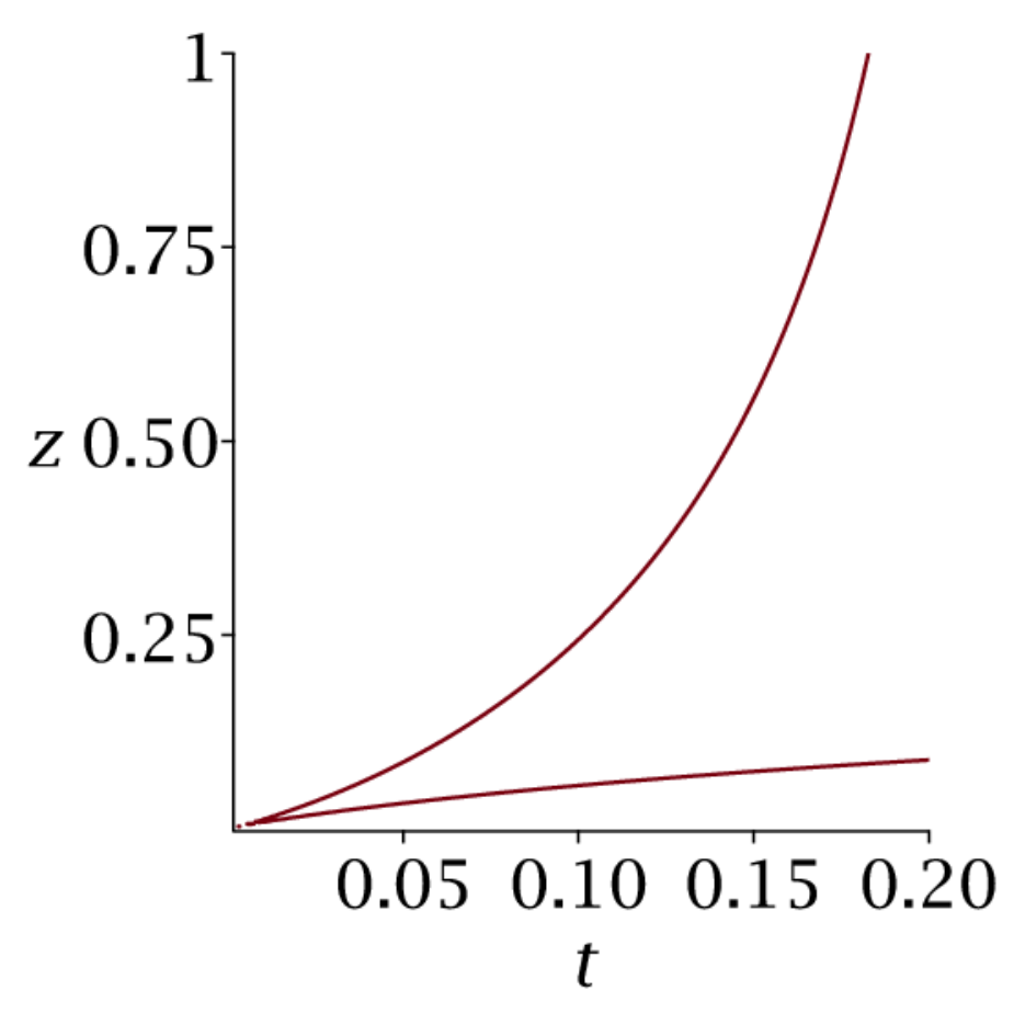
Refer to caption — Figure 8. A plot of $x_{1}(1+x_{1})$ (bottom) and $x_{2}(1+x_{2})$ (top) for $t\in[0,1/5]$ in model #5.

Proof of Theorem 5.7.

Let $\mathcal{S}$ be one of the first eight models of Table 5, and $G(y)$ the associated decoupling function. By Lemma 4.8, the identity

xY_{0}-xY_{1}=G(Y_{0})-G(Y_{1})

holds at the level of formal power series (in $t$ , with rational coefficients in $x$ ). Returning to the analytic framework where $t$ is fixed in $(0,1/|\mathcal{S}|)$ , this identity holds for any $x\in[x_{1},x_{2}]$ (recall from Lemma 5.2 that the curve $\mathcal{L}=Y([x_{1},x_{2}])$ is bounded). By (5.2), any such $x$ thus satisfies $L(Y_{0})=L(Y_{1})$ , where $L(y):=S(y)-G(y)$ . Is $L(y)$ a weak invariant, in the sense of Definition 5.4? By Proposition 5.3, this holds if and only if $p\not\in\mathcal{L}$ . But this is true for $p=0$ by Lemma 5.2, and for $p=-1$ (and model #5) by Lemma 5.8. In both cases, $p$ is in fact in $\mathcal{G}_{\mathcal{L}}$ , and is the only pole of $L(y)$ in this domain. Since it is simple in $G$ , it is also simple in $L$ . Moreover, it is distinct from the pole $y_{2}$ of $w$ , since $y_{2}>0$ (Lemma 5.1) while $p\in\{0,-1\}$ .

Consider now the function $-\frac{rw^{\prime}(p)}{w(y)-w(p)}$ , where $r$ is the residue of $G$ at $p$ . By Proposition 5.5, this is also a weak invariant, with a single pole in $\mathcal{G}_{\mathcal{L}}$ , found at $y=p$ (note that $w^{\prime}(p)$ cannot vanish since $w$ is injective on $\mathcal{G}_{\mathcal{L}}$ ). Its residue at $p$ is $-r$ . Then the invariant lemma (Lemma 5.6) implies that this function differs from $L(y)$ by a constant $c$ :

(5.10)

S(y)-G(y)=c-\frac{rw^{\prime}(p)}{w(y)-w(p)}.

Since both functions have finite limits on $\mathcal{L}$ , this identity holds on $\mathcal{L}$ as well. To conclude the proof of (5.8), it suffices to determine the constant $c$ . Let $\alpha$ be any root of $K(0,y)$ (see Table 8). Since $|\alpha|\leqslant 1$ , $Q(0,y)$ and $S(y)=K(0,y)Q(0,y)$ are analytic in a neighborhood of $\alpha$ , as explained at the beginning of this section, and $S$ vanishes at this point. It remains to expand the above identity at $y=\alpha$ , up to the order $O(y-\alpha)$ , to determine the value of $c$ as given in the theorem.

We now examine the ninth model, which differs from the first eight for two (related) reasons. First, its decoupling function $G$ still has a unique pole (at $p=0$ ) but this pole has order two (see Table 5). Moreover, the curve $\mathcal{L}$ goes through $0$ (Lemma 5.2). However, the idea of the proof is the same as for the first eight models: we will prove that $1/(w(y)-w(p))$ also has a double pole at $0$ , and that subtracting a multiple of this function from $S(y)-G(y)$ yields a pole-free invariant — which is unexpected as there might remain a pole of order $1$ .

So let us examine the function $w(y)$ near $y=0$ . Proposition 5.5 implies that $w$ is analytic in a neighborhood of $0\in\mathcal{L}$ . Let us write $w(y)=\sum_{k\geqslant 0}w_{k}y^{k}$ in this neighborhood. Solving $K(x,y)=0$ in the neighborhood of $x=0$ gives for $Y_{0}$ and $Y_{1}$ the following expansions, valid in $[0,x_{2}]$ (recall that $x_{1}=0$ ):

Y_{0,1}(x)=\pm i\sqrt{x}+\frac{x}{2t}\mp i\frac{x^{3/2}}{8t^{2}}+O(x^{2}).

Since $w$ is an invariant, we have $w(Y_{0})=w(Y_{1})$ for $x\in[0,x_{2}]$ , which forces $w_{1}=0$ , $w_{3}=w_{2}/t$ , and further identities relating the coefficients $w_{k}$ . Moreover, $w_{2}\not=0$ : given the form $w(y)=\wp(\mathcal{Z}(y))$ of (5.4), and the fact that $\mathcal{Z}^{\prime}(0)$ cannot vanish (this follows from the identity (6.10) proved below in Section 6), having $w_{1}=w_{2}=0$ would mean that $\wp^{\prime}$ has a multiple root, namely $\mathcal{Z}(0)$ , which is never true for a Weierstrass function. Hence, around $y=0$ we have:

(5.11)

\frac{w_{2}}{w(y)-w(0)}=\frac{1}{y^{2}}-\frac{1}{ty}-\frac{w_{4}}{w_{2}}+\frac{1}{t^{2}}+O(y).

Let us now compare this to the expansion of $S(y)-G(y)$ near $y=0$ , recalling that $S(0)=0$ :

S(y)-G(y)=\frac{1}{y^{2}}-\frac{1}{ty}+O(y).

This shows that $S(y)-G(y)-w_{2}/(w(y)-w(0))$ is an invariant with no pole on $\mathcal{G}_{\mathcal{L}}$ . Applying Lemma 5.6 implies that this function is constant in $\mathcal{G}_{\mathcal{L}}$ , and the above expansions give this value as $w_{4}/w_{2}-1/t^{2}$ , as stated in (5.9).

5.4. The finite group case

Our approach using weak invariants is robust, and applies to the four (unweighted) decoupled models with a finite group already solved in Section 4 via an algebraic approach.

The method is exactly the same as in Section 5.3, as long as the polynomial $K(0,y)$ has at least one root $\alpha$ . Recall indeed that we used $\alpha$ to identify the constant $c$ in (5.10). As explained below the proof of Lemma 5.2, the existence of $\alpha$ is equivalent to the boundedness of the curve $\mathcal{L}$ , which holds for Kreweras’ model, the double Kreweras’ model and Gessel’s model (Figure 2). In all three cases, the function $S(y)$ is still given by (5.8), where the decoupling function $G(y)$ is given in Table 4, the weak invariant $w(y)$ by (5.4), and the various constants by Table 9. The connection between the weak invariant $w(y)$ and the rational invariant $J(y)$ of Table 2 will be made explicit in Section 8.1.

For the above mentioned three models, an alternative is to proceed as in Sections 3 and 4, up to the point where we construct a series $A(y)$ satisfying the conditions of Lemma 4.18 (for instance $(L(y)-L(0))J(y)-C_{1}L(y)^{3}-C_{2}L(y)^{2}-C_{3}L(y)$ in Section 3), and then apply the analytic invariant lemma (Lemma 5.6) rather than the formal one (Lemma 4.18) to conclude that this series depends on $t$ only.

model
$p$	0	0	$-1$
$r$	$-1$	$-1$	$-1/t$
$\alpha$	$0$	$-1$	$-1$
$g_{0}$	0	1	0

Table 9. Values of

p

r

\alpha

and

g_{0}

for three algebraic models.

Let us now examine what happens in a model for which $K(0,y)=t$ , and solve the reverse Kreweras model (Figure 6, right). We follow the proof of Theorem 5.7. By Proposition 5.3, the function $L(y)=S(y)-G(y)=tQ(0,y)+1/y$ is meromorphic in $\mathcal{G}_{\mathcal{L}}$ , with a unique pole at $0$ , and is bounded at infinity. It is thus an invariant. The analytic invariant lemma tells us that

(5.12)

tQ(0,y)=S(y)=G(y)+\frac{w^{\prime}(0)}{w(y)-w(0)}+c

for some constant $c$ . Since $K(0,y)=t$ has no root (in $y$ ), we cannot use the same trick as in the proof of Theorem 5.7 to determine $c$ . But we can expand the above identity, first at $y=0$ , which gives

S(0)=-\frac{w^{\prime\prime}(0)}{2w^{\prime}(0)}+c,

and then at the unique point $y_{c}\in(0,1)$ such that $K(y,y)=0$ (Figure 9; this point is always in $\mathcal{G}_{\mathcal{L}}$ since $Y(x_{2})=1/\sqrt{x_{2}}>1$ ), which gives

S(y_{c})=G(y_{c})+\frac{w^{\prime}(0)}{w(y_{c})-w(0)}+c.

Now applying (5.1) with $x=y_{c}$ , and using the $x/y$ symmetry of the model, we find that $2S(y_{c})=y_{c}^{2}+S(0)$ . We now use the above expressions of $S(0)$ and $S(y_{c})$ to determine $c$ in terms of $w$ . Returning to (5.12), and using $G(y)=-1/y$ , this finally gives

S(y)=-\frac{1}{y}+\frac{w^{\prime}(0)}{w(y)-w(0)}+y_{c}^{2}+\frac{2}{y_{c}}-\frac{w^{\prime\prime}(0)}{2w^{\prime}(0)}-\frac{2w^{\prime}(0)}{w(y_{c})-w(0)}

for the reverse Kreweras model.

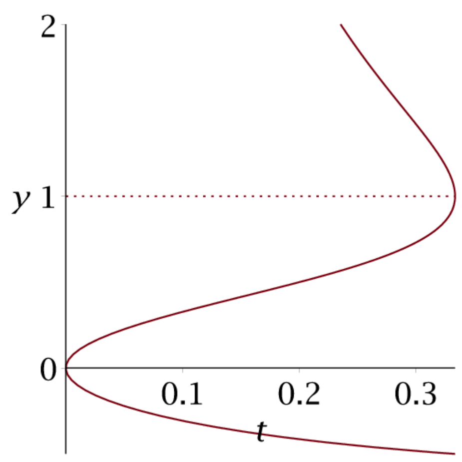
We expect our analytic method to be also applicable to the four weighted algebraic models of Figure 2, right, provided one develops the counterpart of [Ras12] for steps with (real and positive) weights.

6. Differential algebraicity

As recalled in the introduction, quadrant walks have a D-finite generating function if and only if the associated group is finite — we can now say, if and only if they admit rational invariants (Theorem 4.6). Here we will show that the $9$ models with an infinite group that have decoupling functions still satisfy polynomial differential equations. This property will be derived from the new expression for the generating function of these models that we obtained in Section 5 by the analytic invariant approach.

Theorem 6.1.

For any of the $9$ models of Table 5, the generating function $Q(x,y;t)$ is differentially algebraic (or: D-algebraic) in $x,y,t$ . That is, it satisfies three polynomial differential equations with coefficients in $\mathbb{Q}$ : one in $x$ , one in $y$ and one in $t$ .

As discussed in the introduction, this is the first D-algebraicity result for (some) non-D-finite quadrant models [BBMR16], and the 47 other non-D-finite models have been proved to be hypertranscendental since then [DHRS18, DHRS20, DH19].

6.1. Generalities

We consider an abstract differential field $\mathbb{K}$ of characteristic $0$ equipped with one or several derivations. Typical examples occurring in this section are:

•

the field of meromorphic functions in $k$ variables $x_{1},\ldots,x_{k}$ over a complex domain $D$ of $\mathbb{C}^{k}$ , equipped with the derivations $\partial/\partial x_{i}$ ,
•

the quotient field of the (integral) ring of formal power series in the variables $x_{1},\ldots,x_{k}$ with coefficients in $\mathbb{Q}$ , equipped with the derivations $\partial/\partial x_{i}$ ,
•

at the end of the section, the field of Laurent series in $t$ with rational coefficients in $x$ and $y$ , equipped with the three derivations $\partial/\partial t$ , $\partial/\partial x$ and $\partial/\partial y$ .

Definition 6.2.

Let $\mathbb{K}$ be a differential field, with a derivation $\delta$ . An element $F$ of $\,\mathbb{K}$ is $\delta$ -algebraic, if there exists a non-zero polynomial $P(x_{0},x_{1},\ldots,x_{d})$ with coefficients in $\mathbb{Q}$ such that

P(F,\delta F,\ldots,\delta^{(d)}F)=0.

When $F$ is a function or a series involving $k$ variables $x_{1},\ldots,x_{k}$ , as in the above examples, we say that $F$ is differentially algebraic in $x_{i}$ , (or DA in $x_{i}$ ) if it is $\partial/\partial x_{i}$ -algebraic. We say that $F$ is globally DA, (or DA, for short) if it is DA in each of its variables.

It may be surprising that we do not allow polynomial coefficients in the definition of DA series or functions. In fact, this would not enlarge the DA class: indeed, imagine for instance that the series (or function) $F(x,y)$ satisfies a non-trivial equation

P(x,y,F(x,y),\ldots,F^{(d)}(x,y))=0,

where the derivatives are taken with respect to $x$ , and the variable $y$ actually occurs. Then differentiating with respect to $x$ gives another differential equation (DE). If it does not involve $y$ , then we have found a DE that is free from $y$ . Otherwise, we can eliminate $y$ between this new equation and the above one to obtain a DE free from $y$ (the resultant will involve $F^{(d+1)}(x,y)$ , and thus cannot be trivially zero). With one more differentiation, we can similarly construct a DE free from $x$ (and $y$ ) and conclude that $F$ is DA in $x$ .

An important subclass of DA series (or functions) consists of differentially finite series (or functions): We say that $F$ is D-finite in $x_{i}$ (for short: DF in $x_{i}$ ) if there exist polynomials $P_{j}(x_{1},\ldots,x_{k})$ in $\mathbb{Q}[x_{1},\ldots,x_{k}]$ , for $0\leqslant j\leqslant d$ , not all zero, such that

P_{d}(x_{1},\ldots,x_{k})F^{(d)}+\cdots+P_{1}(x_{1},\ldots,x_{k})F^{\prime}+P_{0}(x_{1},\ldots,x_{k})F=0,

where the derivatives are taken with respect to $x_{i}$ . We say that $F$ is globally differentially finite (or D-finite, or DF) if it is DF in each $x_{i}$ . Finally, a simple subclass of DF series (or functions) consists of algebraic elements, that is, series or functions satisfying a non-trivial polynomial equation

P(x_{1},\ldots,x_{k},F)=0

with coefficients in $\mathbb{Q}$ .

The notions of D-finite and D-algebraic series/functions are standard [Lip89, Lip88, Rit50, Sta99], but D-finite series, having a lot of structure, seem to be discussed more often than DA series, at least in the combinatorics literature. Note that if a series is DF (resp. DA), the function that it defines in (say) its polydisc of convergence is also DF (resp. DA). Conversely, any differential equation satisfied in the neighborhood of some point $a=(a_{1},\ldots,a_{k})$ by a function $F$ analytic around $a$ holds at the level of power series for the series expansion of $F$ around $a$ .

We will use a number of closure properties. Some of them can be stated in the context of an abstract differential field, using the following proposition.

Proposition 6.3.

Let $\mathbb{K}$ be a differential field of characteristic $0$ , with a derivation $\delta$ . Let $F\in\mathbb{K}$ . The following statements are equivalent:

(1)

$F$ is $\delta$ -algebraic,
(2)

there exists $d\in\mathbb{N}$ such that all $\delta$ -derivatives of $F$ belong to $\mathbb{Q}(F,\delta F,\ldots,\delta^{(d)}F)$ ,
(3)

there exists a field extension $K$ of $\mathbb{Q}$ of finite transcendence degree that contains $F$ and all its $\delta$ -derivatives,

Proof.

$\ref{it1:DA-equiv}\Rightarrow\ref{it2:DA-equiv}$ . Take a DE for $F$ of minimal order, and minimal total degree among DEs of minimal order:

P(F,\ldots,\delta^{(d)}F)=0.

Applying $\delta$ gives:

\left(\delta^{(d+1)}F\right)P_{1}(F,\ldots,\delta^{(d)}F)+P_{2}(F,\ldots,\delta^{(d)}F)=0

for some polynomials $P_{1}$ and $P_{2}$ . The total degree of $P_{1}$ is less than the total degree of $P$ , and thus by minimality of $P$ , $P_{1}(F,\ldots,\delta^{(d)}F)$ is non-zero. Property (2) then follows by induction on the order of the derivative.

$\ref{it2:DA-equiv}\Rightarrow\ref{it3:DA-equiv}$ . The field $K=\mathbb{Q}(F,F^{\prime},\ldots,\delta^{(d)}F)$ contains all derivatives of $F$ and has transcendence degree at most $d+1$ (recall that $\mathbb{Q}(x_{1},\ldots,x_{k})$ has transcendence degree $k$ ).

$\ref{it3:DA-equiv}\Rightarrow\ref{it1:DA-equiv}$ . If $K$ has transcendence degree $d$ , then the $d+1$ functions $F,F^{\prime},\ldots,\delta^{(d)}F$ are algebraically dependent over $\mathbb{Q}$ .

The following closure properties easily follow.

Corollary 6.4.

The set of $\delta$ -algebraic elements of $\mathbb{K}$ forms a field. This field is closed under $\delta$ , and in fact under any derivation $\partial$ that commutes with $\delta$ .

Proof.

Assume that $F$ and $G$ are $\delta$ -algebraic. Say that all derivatives of $F$ belong to $\mathbb{Q}(F,\ldots,\delta^{(d)}F)$ , and all derivatives of $G$ belong to $\mathbb{Q}(G,\ldots,\delta^{(e)}G)$ . Then all derivatives of $F+G$ and $FG$ belong to $\mathbb{Q}(F,\ldots,\delta^{(d)}F,G,\ldots,\delta^{(e)}G)$ , so that $F+G$ and $FG$ are $\delta$ -algebraic by Proposition 6.3 (3). Similarly, all derivatives of $1/F$ belong to $\mathbb{Q}(F,\ldots,\delta^{(d)}F)$ , so that $1/F$ is $\delta$ -algebraic. The closure under $\delta$ of the field of $\delta$ -algebraic elements is obvious by Proposition 6.3 (2). Finally, if $\partial$ is another derivation commuting with $\delta$ , then $\partial F$ satisfies the same DE as $F$ , and is thus $\delta$ -algebraic.

Specialized to series or functions in $k$ variables $x_{1},\ldots,x_{k}$ , the above corollary implies that $F+G$ , $FG$ , $1/F$ , $\partial F/\partial x_{i}$ are DA as soon as $F$ and $G$ are DA. We will need one final closure property, involving composition.

Proposition 6.5.

If $F(y_{1},\ldots,y_{r})$ is a DA series (or function) of $r$ variables, $G_{1}(x_{1},\ldots,x_{k}),\ldots$ , $G_{r}(x_{1},\ldots,x_{k})$ are DA in all $x_{i}$ ’s, and the composition $H:=F(G_{1},\ldots,G_{r})$ is well defined, then $H$ is DA in the $x_{i}$ ’s.

Proof.

Let us prove that $H$ is DA in $x_{1}$ . If, for $1\leqslant i\leqslant r$ , all $y_{i}$ -derivatives of $F(y_{1},\ldots,y_{r})$ can be expressed rationally in terms of the first $d_{i}$ derivatives, and all $x_{1}$ -derivatives of $G_{j}$ in terms of the first $e_{j}$ ones, then all $x_{1}$ -derivatives of $H$ can be expressed rationally in terms of

•

the functions $\partial^{a}G_{j}/\partial x_{1}^{a}$ , for $1\leqslant j\leqslant r$ and $0\leqslant a<e_{j}$ ,
•

and the functions

$\frac{\partial^{c_{1}+\cdots+c_{k}}F}{\partial y_{1}^{c_{1}}\cdots\partial y_{r}^{c_{r}}}(G_{1},\ldots,G_{k})$

for $0\leqslant c_{i}<d_{i}$ , $1\leqslant i\leqslant r$ . We then apply Proposition 6.3 (3).

D-finiteness is not preserved in general by composition, but we still have the following result (see [Lip89] for a proof in the series setting).

Proposition 6.6.

If $F(y_{1},\ldots,y_{r})$ is a D-finite series (or function) of $r$ variables, $G_{1}(x_{1},\ldots,x_{k})$ , $\ldots,G_{r}(x_{1},\ldots,x_{k})$ are algebraic in the $x_{i}$ ’s, and the composition $H:=F(G_{1},\ldots,G_{r})$ is well defined, then $H$ is D-finite in the $x_{i}$ ’s.

6.2. The Weierstrass elliptic function

It is well known that the Weierstrass function $\wp(z,\omega_{1},\omega_{2})$ defined by (5.6) is DA in $z$ . What may be less known is that it is DA in its periods $\omega_{1}$ and $\omega_{2}$ as well. Since we could not find any reference in the literature, we will sketch a proof.

Proposition 6.7.

The function $\wp(z,\omega_{1},\omega_{2})$ is DA in $z$ , $\omega_{1}$ and $\omega_{2}$ .

Proof.

We refer to [JS87, WW62] for generalities on the Weierstrass function (but we draw the attention of the reader on the fact that the periods are $2\omega_{1}$ and $2\omega_{2}$ in [WW62], instead of $\omega_{1}$ and $\omega_{2}$ (or $\omega_{3}$ ) in our paper). The following differential equation is well known to hold:

\wp_{z}(z,\omega_{1},\omega_{2})^{2}=4\wp(z,\omega_{1},\omega_{2})^{3}-g_{2}(\omega_{1},\omega_{2})\wp(z,\omega_{1},\omega_{2})-g_{3}(\omega_{1},\omega_{2}),

which we shorten as

(6.1)

\wp_{z}^{2}=4\wp^{3}-g_{2}\wp-g_{3},

where $g_{2}$ and $g_{3}$ (also called invariants in the elliptic terminology!) depend on the periods only.

We now use the connection between the Weierstrass function and Jacobi’s theta function:

\theta(z;\tau)=\sum_{n\in\mathbb{Z}}e^{i(2n+1)z+i\pi\tau(n+1/2)^{2}}.

Indeed,

(6.2)

\wp(z,\pi,\pi\tau)=-\frac{\rm{d}}{{\rm d}z}\left(\frac{\theta_{z}(z;\tau)}{\theta(z;\tau)}\right)+\frac{\theta_{zzz}(0;\tau)}{3\theta_{z}(0;\tau)}.

This can be easily proved by observing that the right-hand side of (6.2) has periods $\pi$ and $\pi\tau$ , and behaves like $1/z^{2}+O(z^{2})$ around zero — two properties that characterize $\wp(z,\pi,\pi\tau)$ .

It follows from this and (6.1) that $\theta(z;\tau)$ is DA in $z$ . Hence $\theta(z;\tau)$ and its $z$ -derivatives span a field of finite transcendence degree over $\mathbb{Q}$ . By the heat equation [WW62, Sec. 21.4],

\theta_{\tau}(z;\tau)=-\frac{i\pi}{4}\theta_{zz}(z;\tau),

the $\tau$ -derivatives of $\theta$ are also contained in a field of finite transcendence degree, and $\theta$ is thus DA in $\tau$ . The same holds for any $z$ -derivative of $\theta$ , upon differentiating the heat equation.

It now follows from (6.2) and Corollary 6.4 that $\wp(z,\pi,\pi\tau)$ is DA in $\tau$ as well. Finally, since

\wp(z,\omega_{1},\omega_{2})=\frac{\pi^{2}}{\omega_{1}^{2}}\,\wp\!\left(\frac{\pi z}{\omega_{1}},\pi,\pi\frac{\omega_{2}}{\omega_{1}}\right),

we conclude by Proposition 6.5 that $\wp$ is DA in $\omega_{1}$ and $\omega_{2}$ as well.

6.3. The weak invariant $\boldsymbol{w}$

We now consider a non-singular, unweighted quadrant model. Recall the expression (5.4) of the weak invariant $w(y;t)$ , valid for $t\in(0,1/|\mathcal{S}|)$ and $y$ in the complex domain $\mathcal{G}_{\mathcal{L}}$ , which depends on $t$ (Proposition 5.5). From now on we will often insist on the dependence in $t$ in the notation of our functions, writing for instance $\omega_{1}(t)$ rather than $\omega_{1}$ .

Theorem 6.8.

For any non-singular model, the weak invariant $w(y;t)$ defined by (5.4) can be extended analytically to a domain of $\mathbb{C}^{2}$ where it is D-algebraic in $y$ and $t$ .

Recall that

w(y;t)=\wp\left(\mathcal{Z}(y;t),\omega_{1}(t),\omega_{3}(t)\right),

where the periods $\omega_{1}$ and $\omega_{3}$ are given by (5.7) and the first argument of $\wp$ is

(6.3)

\mathcal{Z}(y;t)=-\frac{\omega_{1}(t)+\omega_{2}(t)}{2}+\wp_{1,2}^{-1}(f(y;t)).

We will argue by composition of DA functions. We have already proved in the previous subsection that $\wp$ is DA in its three arguments. Our next objective will be to prove that $\omega_{1}$ and $\omega_{3}$ are DA in $t$ (and in fact D-finite, see Lemma 6.10). We will then proceed with the bivariate function $\mathcal{Z}$ , which is also D-finite (Lemma 6.11).

As a very first step, we consider the branch points $x_{\ell}$ of $Y_{0,1}$ , and the branch points $y_{\ell}$ of $X_{0,1}$ .

Lemma 6.9.

The functions $x_{1},x_{2},x_{3}$ are algebraic functions of $t$ , and so is $x_{4}$ when it is finite. They are analytic and distinct in a neighborhood of the interval $(0,1/|\mathcal{S}|)$ .

The same holds for the branch points $y_{\ell}$ .

Proof.

The $x_{i}$ ’s are the roots of $d(x)=b(x)^{2}-4a(x)c(x)$ . This is a cubic or quartic polynomial in $x$ , with coefficients in $\mathbb{Q}[t]$ . Its discriminant does not vanish in $(0,1/|\mathcal{S}|)$ since the $x_{i}$ ’s are distinct on this interval (see Lemma 5.1). Its dominant coefficient is easily checked to be $c\,t^{2}$ , for some $c\not=0$ . Since the singularities of algebraic functions are found among the roots of the discriminant and of the dominant coefficient, we conclude that the $x_{i}$ ’s are non-singular on $(0,1/|\mathcal{S}|)$ , and thus (since their singularities are isolated) in a complex neighborhood of this segment.

Lemma 6.10.

The functions $\omega_{1}/i,\omega_{2}$ and $\omega_{3}$ , defined by (5.7) for $t\in(0,1/|\mathcal{S}|)$ , are real and positive. They can be extended analytically in a complex neighborhood of $(0,1/|\mathcal{S}|)$ , where they are D-finite.

Proof.

The periods $\omega_{i}$ are expressed in (5.7) as elliptic integrals. Using the classical reduction to Legendre forms [WW62, Sec. 22.7], we can express them in terms of complete and incomplete elliptic integrals of the first kind, defined respectively, for $k\in(-1,1)$ and $v\in(-1,1)$ , by

K(k)=\int_{0}^{1}\frac{\text{d}y}{\sqrt{1-y^{2}}\sqrt{1-k^{2}y^{2}}}

and

(6.4)

F(v,k)=\int_{0}^{v}\frac{\text{d}y}{\sqrt{1-y^{2}}\sqrt{1-k^{2}y^{2}}}.

Then we claim that:

(6.5)

\omega_{1}=i\alpha\ K\left(\sqrt{\frac{(y_{2}-y_{1})(y_{4}-y_{3})}{(y_{3}-y_{1})(y_{4}-y_{2})}}\right),\qquad\omega_{2}=\alpha\ K\left(\sqrt{\frac{(y_{3}-y_{2})(y_{4}-y_{1})}{(y_{3}-y_{1})(y_{4}-y_{2})}}\right)

and

(6.6)

\omega_{3}=\alpha\ F\left(\sqrt{\frac{(y_{1}-Y(x_{1}))(y_{4}-y_{2})}{(y_{2}-Y(x_{1}))(y_{4}-y_{1})}},\sqrt{\frac{(y_{3}-y_{2})(y_{4}-y_{1})}{(y_{3}-y_{1})(y_{4}-y_{2})}}\right),

where the prefactor $\alpha$ is an algebraic function of $t$ , which depends on the degree ( $3$ or $4$ ) of $\widetilde{d}(y)$ , and of its dominant coefficient $\widetilde{d}_{3}$ or $\widetilde{d}_{4}$ :

(6.7)

\alpha=\begin{cases}\displaystyle\frac{2}{\sqrt{\widetilde{d}_{3}(y_{1}-y_{3})}}&\hbox{if }\widetilde{d}_{4}=0,\\ \displaystyle\frac{2}{\sqrt{\widetilde{d}_{4}(y_{3}-y_{1})(y_{4}-y_{2})}}&\hbox{otherwise}.\end{cases}

The dominant coefficient $\widetilde{d}_{3}$ or $\widetilde{d}_{4}$ is always of the form $\varepsilon ct^{2}$ , with $\varepsilon=\pm 1$ and $c\in\{1,3,4\}$ . The sign $\varepsilon$ equals $+1$ if and only if $y_{4}$ is finite and positive, so that $\alpha$ is always real and positive (see Lemma 5.1 for the properties of the $y_{i}$ ’s).

To obtain the above expressions for the periods, one starts from their original expressions in terms of $\widetilde{d}(y)$ (see (5.7)) and performs the following change of variable in the integrand (for $\omega_{1}$ , $\omega_{2}$ and $\omega_{3}$ respectively):

z=\sqrt{\frac{(y-y_{1})(y_{2}-y_{4})}{(y-y_{4})(y_{2}-y_{1})}},\qquad z=\sqrt{\frac{(y-y_{2})(y_{3}-y_{1})}{(y-y_{1})(y_{3}-y_{2})}},\qquad z=\sqrt{\frac{(y-y_{1})(y_{4}-y_{2})}{(y-y_{2})(y_{4}-y_{1})}}.

The calculation is then straightforward.

If $\widetilde{d}_{4}=0$ , that is, $y_{4}=\infty$ , then the argument of $K$ in (6.5) reduces to $\sqrt{(y_{2}-y_{1})/(y_{3}-y_{1})}$ (resp. $\sqrt{(y_{3}-y_{2})/(y_{3}-y_{1})}$ ) in the expression of $\omega_{1}$ (resp. $\omega_{2}$ ). Similarly, the arguments of $F$ in the expression (6.6) for $\omega_{3}$ are replaced by their limits as $y_{4}\rightarrow\infty$ . Observe that Lemma 5.1 implies that the ratios

\frac{(y_{2}-y_{1})(y_{4}-y_{3})}{(y_{3}-y_{1})(y_{4}-y_{2})}\qquad\hbox{and}\qquad\frac{(y_{3}-y_{2})(y_{4}-y_{1})}{(y_{3}-y_{1})(y_{4}-y_{2})}

are positive. Since they sum to $1$ , they both belong to $(0,1)$ , so that the values of $K$ are well defined in (6.5). A similar argument, relying on Lemma 5.2, proves that the first argument of $F$ in (6.6) lies in $(0,1)$ . The second argument already appears in (6.5).

The function $K(k)$ has a convergent expansion of radius $1$ around $k=0$ :

K(k)=\frac{\pi}{2}\sum_{n\geqslant 0}{2n\choose n}^{2}\left(\frac{k}{4}\right)^{2n}.

It is D-finite, with differential equation

{\displaystyle{\frac{\mathrm{d}}{\mathrm{d}k}}\left[k(1-k^{2}){\frac{\mathrm{d}K(k)}{\mathrm{d}k}}\right]=kK(k)}.

Its only singularities are at $\pm 1$ , and it has an analytic continuation on $\mathbb{C}\setminus((-\infty,-1)\cup(1,+\infty))$ . By Lemma 6.9, the arguments involved in the expressions (6.5) of $\omega_{1}$ and $\omega_{2}$ still have modulus less than 1 in some neighborhood of $(0,1/|\mathcal{S}|)$ , where the $\omega_{i}$ are thus analytic. By Proposition 6.6, these two periods are also D-finite in $t$ .

Let us now return to the expression (6.6) for $\omega_{3}$ . The function $F(v,k)$ has an expansion around $(0,0)$ that converges absolutely for $|v|<1$ and $|k|<1$ :

F(v,k)=\sum_{m,n\geqslant 0}{2m\choose m}{2n\choose n}\frac{k^{2n}}{4^{m+n}}\cdot\frac{v^{2m+2n+1}}{2m+2n+1}.

It is D-finite in each of its two variables (as a bivariate series and thus as a function). Indeed,

(1-v^{2})(1-k^{2}v^{2})\frac{\partial^{2}F}{\partial v^{2}}=v(1+k^{2}-2k^{2}v^{2})\frac{\partial F}{\partial v}

and

3k^{3}v^{2}F+(13k^{4}v^{2}-2k^{2}v^{2}-4k^{2}-1)\frac{\partial F}{\partial k}+k(8k^{4}v^{2}-4k^{2}v^{2}-5k^{2}+1)\frac{\partial^{2}F}{\partial k^{2}}+k^{2}(1-k^{2})(1-k^{2}v^{2})\frac{\partial^{3}F}{\partial k^{3}}=0.

Again, we conclude that $\omega_{3}$ is D-finite in a neighborhood of $(0,1/|\mathcal{S}|)$ by composition with algebraic functions.

Lemma 6.11.

The function $\mathcal{Z}(y;t)$ defined by (6.3) for $t\in(0,1/|\mathcal{S}|)$ and $y\in\mathcal{G}_{\mathcal{L}}$ can be analytically continued to a domain of $\mathbb{C}^{2}$ in which it is D-finite in $t$ and $y$ .

Proof.

In order to understand the nature of $\mathcal{Z}$ , we need to go back to the parametrization of the curve $K(x,y)=0$ by the function $\wp_{1,2}$ . Let us first assume that $y_{4}$ is finite. Then $\wp_{1,2}$ has been constructed in such a way that, for any $z$ , the pair $(x,y)$ defined by

(6.8)		$\displaystyle y$	$\displaystyle=y_{4}+\dfrac{\widetilde{d}^{\prime}(y_{4})}{\wp_{1,2}(z)-\frac{1}{6}\widetilde{d}^{\prime\prime}(y_{4})},$
	$\displaystyle 2\widetilde{a}(y)x+\widetilde{b}(y)$	$\displaystyle=\dfrac{\widetilde{d}^{\prime}(y_{4})\wp_{1,2}^{\prime}(z)}{2(\wp_{1,2}(z)-\frac{1}{6}\widetilde{d}^{\prime\prime}(y_{4}))^{2}},$

satisfies $K(x,y)=0$ (see [FIM99, Lem. 3.3.1] in the probabilistic setting). In other words, if $f(y)=\wp_{1,2}(z)$ , with $f$ defined by (5.5), then (6.8) holds and

(6.9)

\widetilde{d}(y)=\dfrac{(\widetilde{d}^{\prime}(y_{4})\wp_{1,2}^{\prime}(z))^{2}}{4(\wp_{1,2}(z)-\frac{1}{6}\widetilde{d}^{\prime\prime}(y_{4}))^{4}}.

The identity $f(y)=\wp_{1,2}(z)$ holds in particular for $z=\wp_{1,2}^{-1}(f(y))=\mathcal{Z}(y;t)+(\omega_{1}+\omega_{2})/2$ .

Let us now differentiate $\mathcal{Z}$ with respect to $y$ :

\mathcal{Z}^{\prime}(y)=\frac{f^{\prime}(y)}{\wp_{1,2}^{\prime}\circ\wp_{1,2}^{-1}(f(y))}=\frac{f^{\prime}(y)}{\wp_{1,2}^{\prime}(z)}.

Upon squaring this identity, and using first (6.9), and then (6.8), we obtain

(6.10)

\left(\mathcal{Z}^{\prime}(y)\right)^{2}=\frac{(f^{\prime}(y))^{2}}{4\widetilde{d}(y)}\dfrac{(\widetilde{d}^{\prime}(y_{4}))^{2}}{(\wp_{1,2}(z)-\frac{1}{6}\widetilde{d}^{\prime\prime}(y_{4}))^{4}}=\frac{\left(f^{\prime}(y)\right)^{2}}{4\widetilde{d}(y)}\frac{(y-y_{4})^{4}}{\widetilde{d}^{\prime}(y_{4})^{2}}=\frac{1}{4\widetilde{d}(y)}

by definition of $f$ . If $y_{4}$ is infinite (that is, if $\widetilde{d}_{4}=0$ ), then the parametrization of $K(x,y)=0$ is

	$\displaystyle y$	$\displaystyle=\frac{\wp_{1,2}(z)-\widetilde{d}^{\prime\prime}(0)/6}{\widetilde{d}^{\prime\prime\prime}(0)/6},$
	$\displaystyle 2\widetilde{a}(y)x+\widetilde{b}(y)$	$\displaystyle=-\frac{3\wp^{\prime}_{1,2}(z)}{\widetilde{d}^{\prime\prime\prime}(0)},$

and the identity $\left(\mathcal{Z}^{\prime}(y)\right)^{2}=1/(4\widetilde{d}^{\prime}(y))$ still holds.

Another property of the parametrization of the kernel by $\wp_{1,2}$ is that $f(y_{2})=\wp_{1,2}(\frac{\omega_{1}+\omega_{2}}{2})$ (see [Ras12], below (18), recalling that we have swapped the roles of $x$ and $y$ ). Hence, given our convention in the definition of $\wp_{1,2}^{-1}$ in Section 5.2, we have

\mathcal{Z}(y_{2};t)=0.

Finally, recall that $\widetilde{d}(y)$ is real and positive for $y\in(y_{2},y_{3})$ (Lemma 5.1). Hence, for $y\in\mathcal{G}_{\mathcal{L}}\cap[y_{2},y_{3}]$ , it follows from (6.10) that

\mathcal{Z}(y)=-\frac{1}{4}\int_{y_{2}}^{y}\frac{\textnormal{d}u}{\sqrt{\widetilde{d}(u)}}.

(The minus sign comes again from the determination of $\wp_{1,2}^{-1}$ that we have chosen, which has real part in $[0,\omega_{2}/2]$ . Hence the real part of $\mathcal{Z}(y;t)$ is non-positive.) This integral can be expressed in terms of the incomplete elliptic function $F(v,k)$ defined by (6.4), as we did for the period $\omega_{3}$ in the proof of Lemma 6.10:

\mathcal{Z}(y)=-\frac{1}{\alpha}F\left(\sqrt{\frac{(y-y_{2})(y_{3}-y_{1})}{(y-y_{1})(y_{3}-y_{2})}},\sqrt{\frac{(y_{3}-y_{2})(y_{4}-y_{1})}{(y_{3}-y_{1})(y_{4}-y_{2})}}\right),

where the prefactor $\alpha$ is given by (6.7) and the second argument of $F$ is $\sqrt{\frac{y_{3}-y_{2}}{y_{3}-y_{1}}}$ if $y_{4}$ is infinite. Since $F$ is D-finite, and its arguments are algebraic in $t$ , we conclude once again by a composition argument.

6.4. The generating function $\boldsymbol{Q(x,y;t)}$ of decoupled quadrant walks

We now return to the $9$ models with an infinite group for which we have obtained a rational expression for $Q(0,y;t)$ in terms of the weak invariant $w(y;t)$ (Theorem 5.7). We want to prove that the series $Q(x,y;t)$ is D-algebraic (in $t,x$ and $y$ ) for each of them, as claimed in Theorem 6.1.

Let us first prove that $Q(0,y;t)$ is DA. Theorem 5.7 gives an expression for $S(y;t):=K(0,y;t)Q(0,y;t)$ in terms of the weak invariant $w(y;t)$ , valid for $t\in(0,1/|\mathcal{S}|)$ and $y$ in $\mathcal{G}_{\mathcal{L}}$ . By Theorem 6.8, the weak invariant has an analytic continuation on a complex domain, where it is DA. The closure properties of Propositions 6.4 and 6.5 then imply that $S(y;t)$ is also DA, first as a meromorphic function of $y$ and $t$ , then as a series in these variables. The same then holds for $Q(0,y;t)$ .

Let us now go back to $Q(x,0;t)$ , using

R(x):=K(x,0;t)Q(x,0;t)=xY_{0}(x;t)+S(0;t)-S(Y_{0}(x;t);t),

where $Y_{0}(x;t)$ is the root of the kernel that is a power series in $t$ (with coefficients in $\mathbb{Q}[x,\bar{x}]$ ). Again, we conclude that $Q(x,0;t)$ is DA using the closure properties of Propositions 6.4 and 6.5 (since $Y_{0}$ is a series in $t$ with coefficients in $\mathbb{Q}[x,\bar{x}]$ , this is where we take $\mathbb{Q}(x)((t))$ as our differential field, as discussed at the beginning of Section 6.1).

A final application of Proposition 6.4, applied to the main functional equation (2.1), leads us to conclude that $Q(x,y;t)$ is DA as a three-variate series.

6.5. Explicit differential equations in $\boldsymbol{y}$

We now explain how to construct, for the $9$ models of Table 5, an explicit DE in $y$ satisfied by the series $Q(0,y)\equiv Q(0,y;t)$ . This DE has polynomial coefficients in $t$ and $y$ . Depending on the model, the order of this DE ranges from $3$ to $5$ , and the (total) degree in $Q(0,y)$ and its $y$ -derivatives ranges from $2$ to $5$ . We do not claim that it is minimal. The $9$ DEs thus obtained have been checked numerically by expanding $Q(0,y)$ in $t$ up to order $30$ . The corresponding Maple session is available on the authors’ webpages. The construction of explicit DEs in $t$ seems more difficult, as discussed later in Section 8.3.

We start from the expression for $S(y)=K(0,y)Q(0,y)$ given by Theorem 5.7, which can be written as:

(6.11)

K(0,y)Q(0,y)-G(y)=\frac{\alpha}{w(y)-\beta}+\gamma,

for $\alpha$ , $\beta$ and $\gamma$ depending on $t$ only. The weak invariant satisfies a first order DE, derived from (6.1) and (6.10):

(6.12)

4\,\widetilde{d}(y)\left(w^{\prime}(y)\right)^{2}=4w(y)^{3}-g_{2}w(y)-g_{3}.

Here, $g_{2}\equiv g_{2}(\omega_{1},\omega_{3})$ and $g_{3}\equiv g_{3}(\omega_{1},\omega_{3})$ depend (only) on $t$ .

Upon solving (6.11) for $w(y)$ , (6.12) gives a first order DE for $Q(0,y)$ , the coefficients of which are polynomials in $t,y,\alpha,\beta,\gamma,g_{2}$ and $g_{3}$ . By expanding this DE around $y=0$ , we obtain algebraic relations between the 5 unknown series $\alpha,\beta,\gamma,g_{2},g_{3}$ and the series $Q_{0,i}:=\frac{1}{i!}\,\partial^{i}Q/\partial y^{i}(0,0)$ that count walks ending at $(0,i)$ , for $0\leqslant i\leqslant m-1$ (where $m$ depends on the model). We then eliminate $\alpha,\beta,\gamma,g_{2},g_{3}$ to obtain a DE in $y$ that only involves $Q(0,y)$ and the $Q_{0,i}$ , for $0\leqslant i\leqslant m-1$ . For instance, for model #4, we obtain a DE with coefficients in $\mathbb{Q}[t,y,Q_{0,0},Q_{0,1}]$ (hence $m=2$ ), while for model #6, the first $4$ series $Q_{0,i}$ are involved (hence $m=4$ ). Note that this DE is informative: expanding it further around $y=0$ allows one to relate the series $Q_{0,i}$ for $i\geqslant m$ to those with smaller index. For instance, for model #4 we find:

6t^{2}Q_{0,2}=-2{t}^{3}\left({Q_{0,0}}\right)^{2}-4{t}^{2}\,{Q_{0,1}}+3t\,{Q_{0,0}}+{Q_{0,1}}-4t.

Two remarks are in order, regarding models #5 and #9. For model #5, the decoupling function $G(y)$ is singular at $y=-1$ (rather than $y=0$ for the other models), which leads us to write the equation in terms of the $y$ -derivatives of $Q(0,y)$ at $y=-1$ rather than $y=0$ . For model #9, a simplification occurs, since $Q_{0,0}=1+tQ_{0,1}$ (due to the choice of steps), and only two derivatives of $Q(0,y)$ , namely $Q_{0,1}$ and $Q_{0,2}$ , occur in the equation.

At this stage, we can proceed as described below Definition 6.2 to eliminate from the equation the series $Q_{0,i}$ (or $\partial^{i}Q/\partial y^{i}(0,-1)$ for model #5). If $m$ of them actually occur, then the order of the final DE (with coefficients in $\mathbb{Q}[y,t]$ ) will be $m+1$ . For model #4 for instance, for which $m=2$ , we find the following third order DE:

y({t}^{2}{y}^{3}-4{t}^{2}y-2t{y}^{2}-4{t}^{2}+y){\frac{{\rm d}^{3}Q}{{\rm d}{y}^{3}}}(0,y)+(9{t}^{2}{y}^{3}-24{t}^{2}y-15t{y}^{2}-18{t}^{2}+6y){\frac{{\rm d}^{2}Q}{{\rm d}{y}^{2}}}(0,y)\\ -6\left(2{t}^{3}yQ(0,y)-(ty+2t-1)(ty-2t-1)\right){\frac{\rm dQ}{{\rm d}y}}(0,y)-12{t}^{3}Q(0,y)^{2}-6t(5ty-3)Q(0,y)=24t.

Needless to say, we have no combinatorial understanding of this identity. The orders and degrees of the DE obtained for the 9 decoupled models are as follows:

model	#1	#2	#3	#4	#5	#6	#7	#8	#9
order	4	4	4	3	4	5	4	4	3
degree	3	3	4	2	4	5	3	4	2

7. Decoupling functions for other starting points

We have proved in the previous sections that when the function $xy$ is decoupled (in the sense of Definition 4.10), the nature of the series $Q(x,y;t)$ that counts quadrant walks starting at $(0,0)$ tends to be simpler: algebraic when the group $\mathcal{G}(\mathcal{S})$ is finite, D-algebraic otherwise. In this section, we explore the existence of decoupling functions for other starting points. We expect similar implications in terms of the nature of the associated generating function (but we have not worked this out). Remarkably, we find that some infinite group models that are not decoupled for walks starting at $(0,0)$ are still decoupled for other starting points — and we thus expect the associated generating function to be D-algebraic.

For a given model $\mathcal{S}$ , and $a,b\in\mathbb{N}$ , we denote by $q_{a,b}(i,j;n)$ the number of walks in $\mathbb{N}^{2}$ with steps in $\mathcal{S}$ starting at $(a,b)$ and ending at $(i,j)$ . We define the generating function of walks starting at $(a,b)$ by:

Q_{a,b}(x,y)\equiv Q^{\mathcal{S}}_{a,b}(x,y;t)=\sum_{i,j,n\geqslant 0}q_{a,b}(i,j;n)x^{i}y^{j}t^{n}.

This series satisfies the following generalization of (2.1):

K(x,y)Q_{a,b}(x,y)=K(x,0)Q_{a,b}(x,0)+K(0,y)Q_{a,b}(0,y)-K(0,0)Q_{a,b}(0,0)-x^{a+1}y^{b+1}.

This leads us to ask for which models $\mathcal{S}$ and which values of $a$ and $b$ the function $H(x,y):=x^{a+1}y^{b+1}$ is decoupled.

We first give a complete answer in the finite group case (Proposition 7.1). Then we give what we believe to be the complete list of decoupled cases for infinite groups (Proposition 7.2). We conclude in Proposition 7.3 with the 4 weighted models of Figure 2.

Remarks
1. Clearly, if a model $\mathcal{S}$ with starting point $(a,b)$ is decoupled, then the model obtained after reflection in the first diagonal is decoupled for $(b,a)$ . Hence the “complete answer” and “complete list” mentioned above are complete up to diagonal symmetry.
2. If for some model $\mathcal{S}$ the series $Q^{\mathcal{S}}_{a,b}(x,y)$ is algebraic (resp. D-algebraic), then for all $(c,d)\in\mathbb{N}^{2}$ , the coefficient of $x^{c}y^{d}$ in this series is also (D-)algebraic. This series counts quadrant walks with steps in $\mathcal{S}$ going from $(a,b)$ to $(c,d)$ , or, upon reversing steps, quadrant walks from $(c,d)$ to $(a,b)$ with steps in $\overline{\mathcal{S}}:=\{(-i,-j):(i,j)\in\mathcal{S}\}$ . This means that the coefficient of $x^{a}y^{b}$ in $Q^{\overline{\mathcal{S}}}_{c,d}(x,y)$ is (D-)algebraic for all $c,d$ . For instance, for each model $\mathcal{S}$ of Table 4 (resp. 5), and each starting point $(c,d)$ , the series $Q^{\overline{\mathcal{S}}}_{c,d}(0,0)$ is algebraic (resp. D-algebraic). But what we have in mind in this section is the (D-)algebraicity of the three-variate series $Q^{\overline{\mathcal{S}}}_{c,d}(x,y)$ .

7.1. Models with a finite group

Proposition 7.1.

Let $\mathcal{S}$ be one of the $23$ unweighted models with a finite group, listed in [BMM10, Tables 1–3]. Let $H(x,y):=x^{a+1}y^{b+1}$ , with $(a,b)\in\mathbb{N}^{2}$ .

(1)

If $\mathcal{S}$ is none of the models of Figure 2 (the Kreweras trilogy and Gessel’s model), then $H(x,y)$ is not decoupled.
(2)

If $\mathcal{S}$ belongs to the Kreweras trilogy, then $H(x,y)$ is decoupled if and only if $a=b$ .
(3)

If $\mathcal{S}$ is Gessel’s model, then $H(x,y)$ is decoupled if and only if either $a=b$ or $a=2b+1$ .

Proof.

Recall from Theorem 4.11 that $H(x,y)$ is decoupled if and only if $H_{\alpha}(x,y)=0$ , where $\alpha=\sum_{\gamma\in\mathcal{G}(\mathcal{S})}\sign(\gamma)\gamma$ . We refer to [BMM10, Tables 1–3] for the explicit description of the group $\mathcal{G}(\mathcal{S})$ . We will use the following notation: for a Laurent polynomial $P$ in a variable $z$ , we denote by $[z^{>}]P$ (resp. $[z^{<}]P$ ) the sum of monomials of positive (resp. negative) exponents in $z$ . We call it the positive (resp. negative) part of $P$ in $z$ .

Let us first consider Gessel’s model. The group $\mathcal{G}(\mathcal{S})$ has order 8 and

H_{\alpha}(x,y)={H}(x,y)-{H}\left({\bar{x}\bar{y}},y\right)+{H}\left({\bar{x}\bar{y}},x^{2}y\right)-{H}\left({\bar{x}},x^{2}y\right)\\ +H(\bar{x},\bar{y})-H(xy,\bar{y})+H(xy,\bar{x}^{2}\bar{y})-H(x,\bar{x}^{2}\bar{y}),

It is easy to check that if $a=b$ or $a=2b+1$ , then $H_{\alpha}(x,y)=0$ . Conversely,

•

if $a<b$ , then $[x^{>}][y^{<}]H_{\alpha}(x,y)=-x^{a+1}y^{a-b}\neq 0$ ,
•

if $b<a<2b+1$ , then $[x^{>}][y^{<}]H_{\alpha}(x,y)=x^{2b-a+1}y^{b-a}\neq 0$ ,
•

and $2b+1<a$ , then $[x^{>}][y^{<}]H_{\alpha}(x,y)=-x^{a-2b-1}y^{-b-1}\neq 0$ ,

hence $H(x,y)$ is not decoupled. This proves Claim (3).

Claims (1) and (2) are proved in a similar fashion. For instance, for the $16$ models having a vertical symmetry,

H_{\alpha}(x,y)=H(x,y)-H\left({\bar{x}},y\right)+H\left({\bar{x}},\bar{y}\,\frac{c(x)}{a(x)}\right)-H\left(x,\bar{y}\,\frac{c(x)}{a(x)}\right),

where as before $a(x)=[y^{2}]K(x,y)$ and $c(x)=[y^{0}]K(x,y)$ . Thus $H_{\alpha}(x,y)$ is a Laurent polynomial in $y$ , with positive part $H(x,y)-H\left({\bar{x}},y\right)$ , and finally,

[x^{>}][y^{>}]H_{\alpha}(x,y)=x^{a+1}y^{b+1}\neq 0,

showing that $H(x,y)$ is never decoupled.

One can also give explicit decoupling functions for the four algebraic models: upon generalizing Lemma 4.8 to the function $H(x,y)=x^{a+1}y^{a+1}$ , we can check that all four models admit $F(x)=-x^{-a-1}$ as $x$ -decoupling function. Similarly, for Gessel’s model with starting point $(2b+1,b)$ , a $y$ -decoupling function is $G(y)=-y^{-b-1}$ .


$(a,a)$	$(a,a)$	$(a,a)$	$(a,a)$	$(0,0)$	$(a,a)$	$(a,a)$	$(0,0)$
			$(2b+1,b)$				$(1,0)$

Table 10. Exhaustive list of decoupled cases among models with a finite group (left) and among the 4 weighted models of Figure 2.

Remarks
1. We recall from [BMM10, Prop. 8] that the $19$ models that never decouple (case (1) above) can be solved by extracting the positive part (in $x$ and $y$ ) in the alternating sum $\widetilde{Q}_{\alpha}(x,y)$ , where $\widetilde{Q}(x,y)=xyQ(x,y)$ . Indeed, this positive part turns out to be simply $xyQ(x,y)$ . This property is closely related to the above extraction procedure, and to the non-existence of decoupling functions.
2. Given a step set $\mathcal{S}$ , one can also ask whether a linear combination $\sum_{a,b}c_{a,b}Q_{a,b}(x,y)$ is (D-)algebraic. This makes sense for instance in a probabilistic setting, where the $c_{a,b}$ ’s describe an initial law for the starting point. Again, we expect this to be equivalent to the polynomial $H(x,y):=\sum_{a,b}c_{a,b}x^{a+1}y^{b+1}$ being decoupled. We can extend the proof of Proposition 7.1 to study this question. If $\mathcal{S}$ is one of the $19$ models listed in (1), then $H(x,y)$ is never decoupled. If $\mathcal{S}$ is one of the Kreweras-like models, then $H(x,y)$ is decoupled if and only if $c_{a,b}=c_{b,a}$ for all $(a,b)$ . For instance, we expect $Q_{0,1}+Q_{1,0}$ to be algebraic. The condition is a bit more complex in Gessel’s case.
3. As discussed above, the existence of a decoupling function for a finite group model does not imply algebraicity in a completely automatic fashion, and further work is required to prove it. We have done this for Kreweras’ walks starting anywhere on the diagonal: the associated generating function, which involves one more variable recording the position of the starting point, is indeed still algebraic.

7.2. Models with an infinite group

We now address models with an infinite group, and exhibit decoupling functions in a number of cases. Remarkably, we find that three models that are not decoupled for walks starting at $(0,0)$ still admit decoupling functions for other starting points. This contrasts with the finite group case.

Proposition 7.2.

Let $\mathcal{S}$ be one of the $12$ models with an infinite group shown in Table 11. Then the function $x^{a+1}y^{b+1}$ is decoupled for the values of $(a,b)$ shown in the corresponding column.

Based on an (incomplete) argument and a systematic search (for $a,b\leqslant 10$ ), we believe these values of $(\mathcal{S},a,b)$ to be the only decoupled cases (for infinite groups).


$(a,a)$	$(0,0)$	$(a,a)$	$(0,0)$	$(a,a)$	$(a,a)$	$(0,0)$	$(0,0)$	$(0,0)$
		$(0,1)$		$(0,1)$	$(0,1)$				$(0,1)$	$(0,1)$	$(0,1)$
				$(1,0)$
				$(1,3)$				$(1,1)$

Table 11. A (conjecturally exhaustive) list of decoupled cases among models with an infinite group.

Proof.

Consider a model with kernel $K(x,y)$ , and take a rational function $H(x,y)$ . Lemma 4.8 can be readily extended to show that the following conditions are equivalent:

(a)

$H(x,y)$ is decoupled, that is, there exist rational functions $F(x),G(y)$ such that $K(x,y)$ divides $H(x,y)-F(x)-G(y)$ ,
(b)

there exists a rational function $F(x)$ such that $H(X_{0},y)-F(X_{0})=H(X_{1},y)-F(X_{1})$ , where $X_{0},X_{1}$ are the roots of $K(x,y)$ (when solved for $x$ ),
(c)

there exists a rational function $G(y)$ such that $H(x,Y_{0})-G(Y_{0})=H(x,Y_{1})-G(Y_{1})$ , where $Y_{0},Y_{1}$ are the roots of $K(x,y)$ (when solved for $y$ ).

We call $x$ -decoupling function (resp. $y$ -decoupling function) of $H(x,y)$ a rational function $F(x)$ (resp. $G(y)$ ) satisfying Condition (b) (resp. Condition (c)).

We begin with the starting point $(a,a)$ . When $a=0$ , we have proved that the $9$ decoupled models with an infinite group are those numbered from #1 to #9. Now let $a$ be arbitrary, and denote $H(x,y)=x^{a+1}y^{a+1}$ . For models #3 and #5, we have $\frac{1}{X_{0}X_{1}}=y$ . Hence,

H(X_{0},y)-H(X_{1},y)=\frac{X_{0}^{a+1}}{(X_{0}X_{1})^{a+1}}-\frac{X_{1}^{a+1}}{(X_{0}X_{1})^{a+1}}=\frac{1}{X_{1}^{a+1}}-\frac{1}{X_{0}^{a+1}}.

This shows that $F(x)=-x^{-a-1}$ is an $x$ -decoupling function for $H(x,y)$ . Similarly, for models #1 and #6, one has $\frac{1}{Y_{0}Y_{1}}=x$ , so that $G(y)=-y^{-a-1}$ is a $y$ -decoupling function for $H(x,y)$ . Finally, for $a=1$ and model #9, one easily checks that the function

G(y)={y}^{4}-2{\frac{{y}^{3}(1+2t)}{t}}+{\frac{{y}^{2}(5{t}^{2}+4t+1)}{{t}^{2}}}\\ -2{\frac{y(1+2t)(1+t)}{{t}^{2}}}-2{\frac{(1+t)^{2}}{{t}^{2}y}}+{\frac{2{t}^{2}+2t+1}{{t}^{2}{y}^{2}}}-{\frac{2}{t{y}^{3}}}+\frac{1}{y^{4}}

is a $y$ -decoupling function for $H(x,y)$ .

Next we consider the starting point $(0,1)$ , that is, $H(x,y)=xy^{2}$ . For model #3, one can take $F(x)=-x-\frac{1}{xt}+\frac{1}{x^{2}}$ . For model #5, one may take $F(x)={x}^{2}-{\frac{x}{t}}-{\frac{1+t}{tx}}+\frac{1}{x^{2}}$ . For model #6, one can take $F(x)=x+\frac{1+t}{t^{2}(1+x)}-\frac{(1+t)^{2}}{t^{2}(1+x)^{2}}$ . For models #10 and #12, one can take $F(x)=-x-1/x$ . For model #11, one can take $F(x)=-x-1/(tx)+1/x^{2}$ .

Now we consider model #5 and the starting point $(1,0)$ , that is, $H(x,y)=x^{2}y$ . Then one can take $F(x)=\frac{x}{t}-x^{2}+\frac{1}{x}$ .

Finally, for $(a,b)=(1,3)$ and model #5, we can check that

F(x)=-{x}^{4}+2{\frac{{x}^{3}}{t}}-{\frac{{x}^{2}(2{t}^{2}+2t+1)}{{t}^{2}}}+2{\frac{x(1+t)^{2}}{{t}^{2}}}\\ +2{\frac{(1+2t)(1+t)}{x{t}^{2}}}-{\frac{5{t}^{2}+4t+1}{{x}^{2}{t}^{2}}}+2{\frac{1+2t}{{x}^{3}t}}-\frac{1}{x^{4}}

is an $x$ -decoupling function for $H(x,y)=x^{2}y^{4}$ .

7.3. Weighted models with a finite group

Proposition 7.3.

Consider the four weighted models of Figure 2. The list of starting points $(a,b)$ for which they decouple is given in Table 10. Specializing $\lambda$ to some complex value in the first model does not yield more decoupled cases.

Proof.

We denote as before $H(x,y)=x^{a+1}y^{b+1}$ . The first weighted model has a group of order $6$ . Writing $y=z-1$ makes its elements more compact, and we find:

H_{\alpha}(x,z-1)=H(x,z-1)-H\left({\frac{1}{xz}},z-1\right)+H\left({\frac{1}{xz}},{\frac{{x}^{2}{z}^{2}+\lambda\,xz+1}{z-1}}\right)\\ -H\left({\frac{x\left(z-1\right)}{{x}^{2}z+\lambda\,x+1}},{\frac{{x}^{2}{z}^{2}+\lambda\,xz+1}{z-1}}\right)+H\left({\frac{x\left(z-1\right)}{{x}^{2}z+\lambda\,x+1}},{\frac{\lambda\,x+{x}^{2}+1}{{x}^{2}\left(z-1\right)}}\right)-H\left(x,{\frac{\lambda\,x+{x}^{2}+1}{{x}^{2}\left(z-1\right)}}\right).

Setting $z=x$ in this expression and taking the limit $x\to\infty$ , we find

H_{\alpha}(x,x-1)=x^{a+b+2}-x^{3b-a+2}+o(x^{a+b+2}+x^{3b-a+2}).

For $H(x,y)$ to be decoupled, we need $H_{\alpha}(x,x-1)=0$ , which forces $a=b$ . Under this assumption we further obtain

H_{\alpha}(x,x-1)=-(a+1)x^{2a+1}+x^{a+1}+o(x^{2a+1}+x^{a+1}),

which now forces $a=b=0$ . Conversely, if $(a,b)=(0,0)$ then $H(x,y)$ is decoupled as proved in Section 4.2.

The second weighted model has a group of order $10$ , and

H_{\alpha}(x,y)=\widetilde{H}(x,y)-\widetilde{H}\left({\frac{y}{x(1+y)}},y\right)+\widetilde{H}\left({\frac{y}{x(1+y)}},\frac{1}{xy+x+y}\right)\\ -\widetilde{H}\left({\frac{x}{y(x+1)}},\frac{1}{xy+x+y}\right)+\widetilde{H}\left({\frac{x}{y(x+1)}},x\right),

where $\widetilde{H}(x,y)=H(x,y)-H(y,x)$ . Setting $y=x^{2}$ and taking the limit at $x\to\infty$ , we find

H_{\alpha}(x,x^{2})=x^{a+2b+3}-x^{2a+b+3}+o(x^{a+2b+3}-x^{2a+b+3}).

Hence $H_{\alpha}(x,y)=0$ implies $a=b$ . Conversely, if $a=b$ , then $\widetilde{H}(x,y)=0$ , so $H_{\alpha}(x,y)=0$ . The proof for the third model is similar (except that it is easier to expand of $H_{\alpha}(x,x^{2})$ at $x=0$ ).

Lastly, the fourth model has a group of order 10, and

H_{\alpha}(x,y)=\widehat{H}(x,y)-\widehat{H}\left({\frac{1+y}{xy}},y\right)+\widehat{H}\left({\frac{1+y}{xy}},{\frac{x}{xy+y+1}}\right)\\ -\widehat{H}\left(y(x+1),{\frac{x}{xy+y+1}}\right)+\widehat{H}\left(y(x+1),\frac{1}{x}\right),

where $\widehat{H}(x,y)=H(x,y)-H(\bar{y},\bar{x})$ . Setting $y=x^{2}$ and taking the limit $x\to\infty$ , we find

H_{\alpha}(x,x^{2})=x^{a+2b+3}+x^{3a-b+2}-x^{2a+b+3}+o(x^{a+2b+3}+x^{3a-b+2}+x^{2a+b+3}).

Hence $H_{\alpha}(x,y)=0$ implies either $a=b$ or $a=2b+1$ . In both cases, expanding further $H_{\alpha}(x,x^{2})$ as $x\to\infty$ leads to $b=0$ . Hence either $(a,b)=0$ (and then we know that the model decouples), or $(a,b)=(1,0)$ . We conclude by checking that indeed, $H_{\alpha}(x,y)=0$ for $H(x,y)=x^{2}y$ .

Remark. As in the infinite group case, there exist weighted models that do not decouple at $(0,0)$ , but do decouple at other starting points. For instance, the model obtained by reversing all steps of the first weighted model decouples at $(1,0)$ when $\lambda=0$ . This model is of interest in the study of 3-dimensional walks confined to the first octant [BBMKM16, Sec. 8.2].

8. Final comments and questions

We begin here with two comments on our results. In the first subsection, we relate weak and rational invariants. In the second one, we discuss the link between our new expressions for $Q(0,y)$ (Theorem 5.7) and the integral expressions formerly obtained in [Ras12]. We then go on with a list of open questions and perspectives (Sections 8.3 to 8.6).

8.1. Weak invariants vs. rational invariants in the finite group case

In the finite group case — and in this case only — we were able to exhibit both a rational invariant $J(y)$ (Definition 4.3) and a weak invariant $w(y)$ (Definition 5.4). The weak invariant $w(y)$ is more intrinsic than the rational invariant $J(y)$ : indeed, the analytic invariant lemma (Lemma 5.6) together with Proposition 5.5 implies that many invariants, as $S(y)-L(y)$ in Section 5, have a rational expression in terms of $w(y)$ . On the other hand, $w(y)$ depends on $t$ and $y$ in a more complex fashion than $J(y)$ . Indeed, $w(y)$ is known to be algebraic in $y$ (and in fact rational in $19$ cases), see [Ras12, Thm. 3]; moreover, it is D-algebraic in $t$ by Theorem 6.8. In fact it can even be proved to be algebraic in $t$ (in the finite group case), but still not as simple as $J(y)$ .

In this section, we show how to relate $J(y)$ and $w(y)$ using the analytic invariant lemma.

Let us first consider one of the $16$ models with a horizontal symmetry, for which a rational invariant is $J(y):=y+1/y$ . One can check that the curve $\mathcal{L}$ is the unit circle (see [FIM99, Thm. 5.3.3 (i)] for the probabilistic case $t=1/|\mathcal{S}|$ ) and in particular the pole $y=0$ never lies on $\mathcal{L}$ . Hence $J(y)$ is a weak invariant, in the sense of Definition 5.4. Applying the analytic invariant lemma shows that

J(y)=\frac{w^{\prime}(0)}{w(y)-w(0)}+\frac{w^{\prime\prime}(0)}{2w^{\prime}(0)}.

In particular, we have thus rederived the fact that $w(y)$ is rational in $y$ .

Figure 10. The three D-finite transcendental models that have no horizontal nor vertical symmetry.

We now address the three models that have no horizontal symmetry and have a transcendental generating function (Figure 10). For the first one, $J(y)=ty^{2}-y-t/y$ has a single pole at $0$ . The curve $\mathcal{L}$ is bounded and $\mathcal{G}_{\mathcal{L}}$ contains $0$ , so that

J(y)=-\frac{t\,w^{\prime}(0)}{w(y)-w(0)}+\gamma,

for some $\gamma$ that depends on $t$ only.

For the second model, $J(y)=\frac{y}{t(1+y)^{2}}+t\frac{(1+y)^{2}}{y}$ (as in Gessel’s model) has a simple pole at $0\in\mathcal{G}_{\mathcal{L}}$ and a double pole at $-1\not\in\mathcal{L}\cup\mathcal{G}_{\mathcal{L}}$ . The invariant lemma gives

J(y)=\frac{t\,w^{\prime}(0)}{w(y)-w(0)}+\gamma.

Finally for the third model, $J(y)=t/y-yt-(2t+1)/(y+1)$ has a simple pole at $0\in\mathcal{G}_{\mathcal{L}}$ and another one at $-1\not\in\mathcal{L}\cup\mathcal{G}_{\mathcal{L}}$ , and the previous expression $J$ in terms of $w$ holds as well.

Let us now address the four algebraic models, for which invariants are given in Table 2. For Kreweras’ model, $J(y)$ has a double pole at $0$ , and the invariant lemma results in:

J(y)=\frac{t}{y^{2}}-\frac{1}{y}-ty=\frac{t\,w^{\prime}(0)^{2}}{(w(y)-w(0))^{2}}+\frac{\beta}{w(y)-w(0)}+\gamma,

showing that $w(y)$ is quadratic in $y$ .

For reverse Kreweras walks, the curve $\mathcal{L}$ is not bounded, and the invariant $J(y)=ty^{2}-y-t/y$ is not bounded at infinity. Hence we cannot apply directly Lemma 5.6. However, it follows from Lemma 8.1 (proved below) that

(8.1)

J(y)=\frac{\alpha}{w(y)-w(\infty)}-\frac{t\,w^{\prime}(0)}{w(y)-w(0)}-\gamma.

This shows that $w(y)$ is quadratic in $y$ .

For the double Kreweras model, $J(y)$ has two poles, at $0$ and at $-1$ . Both belong to $\mathcal{G}_{\mathcal{L}}$ , and the invariant lemma results in:

J(y)=\frac{t}{y}-ty-\frac{1+2t}{1+y}=\frac{\alpha}{w(y)-w(0)}+\frac{\beta}{w(y)-w(-1)}+\gamma,

showing that $w(y)$ is again quadratic in $y$ .

Finally, for Gessel’s model, $J(y)$ has poles at $0$ and $-1$ , both belonging to $\mathcal{G}_{\mathcal{L}}$ , and respectively simple and double. The invariant lemma gives

J(y)=\frac{y}{t(1+y)^{2}}+t\bar{y}(1+y)^{2}=\frac{\alpha}{(w(y)-w(-1))^{2}}+\frac{\beta}{w(y)-w(-1)}+\frac{\gamma}{w(y)-w(0)}+\delta,

showing that $w(y)$ is (at most) cubic in $y$ .

We conclude this section with the lemma used above for reverse Kreweras walks (see (8.1)).

Lemma 8.1.

If the curve $\mathcal{L}$ is unbounded, then the weak invariant $w(y)$ is analytic at infinity, where the following expansion holds:

\frac{w_{2}}{w(y)-w(\infty)}=y^{2}-\frac{y}{t}+O(1)

for some $w_{2}\not=0$ .

(This lemma is essentially a version of the identity (5.11) that we wrote for model #9, with the point $0$ replaced by $\infty$ .)

Proof.

If $\mathcal{L}$ is unbounded then the branch point $x_{1}$ is zero, and none of the steps $(-1,0)$ and $(-1,1)$ belong to $\mathcal{S}$ (Lemma 5.2). This forces $(-1,-1)$ and $(0,1)$ to be in $\mathcal{S}$ . Solving the kernel for $y$ gives, as $x\rightarrow 0$ ,

(8.2)

Y_{0,1}(x)=\pm\frac{i}{\sqrt{x}}+\frac{1}{2t}+O(\sqrt{x}).

Let us return to the form $w(y)=\wp_{1,3}(\mathcal{Z}(y))$ of (5.4). The parametrization of the curve $K(x,y)$ by $\wp_{1,2}$ has been designed so that $f(Y(x_{1}))=\wp_{1,2}((\omega_{2}-\omega_{3})/2)$ , see [KR12, Sec. 3.2], which in our case reads $f(\infty)=\widetilde{d}^{\prime\prime}(y_{4})/6=\wp_{1,2}((\omega_{2}-\omega_{3})/2)$ (it is readily checked that $y_{4}$ is finite under our hypotheses). Hence $\mathcal{Z}(\infty)=-(\omega_{1}+\omega_{3})/2$ , which is a zero of $\wp_{1,3}^{\prime}$ , but not a pole of $\wp_{1,3}$ . Thus $w$ is analytic at infinity. Let us denote

w(y)=w(\infty)+\frac{w_{1}}{y}+\frac{w_{2}}{y^{2}}+\frac{w_{3}}{y^{3}}+O\left(\frac{1}{y^{4}}\right).

Writing that $w(Y_{0})=w(Y_{1})$ near $x=0$ , with the $Y_{k}(x)$ ’s given by (8.2), we obtain $w_{1}=0$ and $w_{3}=w_{2}/t$ . As in the proof of (5.11), the fact that $w_{2}\not=0$ comes from the fact that $\mathcal{Z}(\infty)=-(\omega_{1}+\omega_{3})/2$ is a zero of $\wp_{1,3}^{\prime}$ but not of its derivative. The lemma then follows.

8.2. A connection with integral representations of $\boldsymbol{Q(x,y)}$

Prior to this paper, for a non-singular model with an infinite group, the series $Q(x,y)$ was expressed as a contour integral involving the gluing function $w(y)$ (a.k.a. weak invariant) [Ras12]. If the model has a decoupling function, we have now obtained a simpler, integral-free expression in Theorem 5.7. We explain here, without giving all details, how to derive it from the integral one, in the analytic setting of Section 5. To avoid technicalities we only consider models such that $0\notin[x_{1},x_{2}]$ , thereby excluding models #2, #7 and #9.

Let $\widehat{w}(x)$ be the counterpart of the weak invariant $w(y)$ , but for the variable $x$ . In particular, $\widehat{w}(x)$ is a gluing function for the domain $\mathcal{G}_{\mathcal{M}}$ already introduced in the proof of Proposition 5.3. Then, for $x\in\mathcal{G}_{\mathcal{M}}\setminus[x_{1},x_{2}]$ , it is known that

(8.3)

R(x)-R(0)=xY_{0}(x)+\frac{1}{2\pi i}\int_{x_{1}}^{x_{2}}u(Y_{0}(u-0i)-Y_{1}(u-0i))\left\{\frac{\widehat{w}^{\prime}(u)}{\widehat{w}(u)-\widehat{w}(x)}-\frac{\widehat{w}^{\prime}(u)}{\widehat{w}(u)-\widehat{w}(0)}\right\}\text{d}u,

where $Y_{k}(u\pm 0i)$ stands for $\lim Y_{k}(x)$ when $x\to u$ with $\Im(\pm x)>0$ . This is Theorem 1 in [Ras12], stated here with greater precision (indeed, the first term in the integrand is written as $Y_{0}(u)-Y_{1}(u)$ in [Ras12]). Recall from Subsection 5.1 that the functions $Y_{0}$ and $Y_{1}$ are not meromorphic on $[x_{1},x_{2}]$ , but admit limits from above and below. These limits satisfy

(8.4)

Y_{0}(u\pm 0i)=\overline{Y_{1}(u\pm 0i)},\quad\Im(Y_{0}(u-0i))>0,\quad\Im(Y_{0}(u+0i))<0.

More details can be found in the proof of [Ras12, Thm. 1], or in [KR11, Sec. 4] for Gessel’s model. Note that the assumption $0\not\in[x_{1},x_{2}]$ guarantees that the term $\widehat{w}(u)-\widehat{w}(0)$ does not vanish. When $x\in[x_{1},x_{2}]$ , and more generally when $x$ is in the unit disk, $R(x)$ is analytic, even though the two terms of (8.3) are not analytic along this interval.

The first crucial point is that we can replace $\widehat{w}$ by ${w}(Y_{0})$ in (8.3), where $w$ is the gluing function (5.4) for $\mathcal{G}_{\mathcal{L}}$ . This comes from a combination of three facts:

•

as demonstrated in [Ras12, Thm. 6], ${w}(Y_{0}(x))$ is a conformal gluing function for $\mathcal{G}_{\mathcal{M}}$ , in the sense that it satisfies Proposition 5.5 — except that we are now in the $x$ variable, and that the pole is located at $X(y_{2})$ rather than $x_{2}$ (note that the invariance property $w(Y_{0}(x))=w(Y_{1}(x))$ spares us the trouble of taking upper or lower limits when defining $w(Y_{0}(x))$ for $x\in[x_{1},x_{2}]$ );
•

any two conformal gluing functions $w_{1}$ and $w_{2}$ are related by a homography. That is, $w_{1}=\frac{aw_{2}+b}{cw_{2}+d}$ , for some coefficients $a,b,c,d\in\mathbb{C}$ (depending on $t$ ) such that $ad-bc\neq 0$ , see [Ras12, Rem. 6];
•

the quantity

$\frac{\widehat{w}^{\prime}(u)}{\widehat{w}(u)-\widehat{w}(x)}-\frac{\widehat{w}^{\prime}(u)}{\widehat{w}(u)-\widehat{w}(0)}$

in the right-hand side of (8.3) takes the same value, should $\widehat{w}$ be replaced by $\frac{a\widehat{w}+b}{c\widehat{w}+d}$ .

Now assume that the model admits a (rational) decoupling function $G$ . Then $u(Y_{0}(u)-Y_{1}(u))=G(Y_{0}(u))-G(Y_{1}(u))$ (Lemma 4.8). The integral in (8.3) thus becomes:

\frac{1}{2\pi i}\int_{x_{1}}^{x_{2}}\left(G(Y_{0}(u-0i))-G(Y_{1}(u-0i))\right)D(Y_{0}(u))\,Y_{0}^{\prime}(u)\text{d}u,

with

{D(v)=\frac{{w}^{\prime}(v)}{{w}(v)-{w}(Y_{0}(x))}-\frac{{w}^{\prime}(v)}{{w}(v)-{w}(Y_{0}(0))}.}

Again, the invariant condition $w(Y_{0}(u+0i))=w(Y_{0}(u-0i))$ for $u\in[x_{1},x_{2}]$ allows us to replace $u$ by $u\pm 0i$ in the term $D(Y_{0}(u))Y_{0}^{\prime}(u)$ above.

Let us write the above integral as a difference $T_{0}-T_{1}$ of two terms, one (namely $T_{0}$ ) involving $G(Y_{0}(u-0i))$ and the other one $T_{1}$ involving $G(Y_{1}(u-0i))$ . Recall that $Y(x_{1})\leqslant 0$ and $Y(x_{2})>0$ (Lemma 5.2), and the properties (8.4). The change of variable $v=Y_{0}(u-0i)$ in $T_{0}$ gives

T_{0}=\frac{1}{2\pi i}\int_{\mathcal{L}\cap\{v:\Im(v)\geqslant 0\}}G(v){D(v)}\text{d}v,

where the contour is oriented clockwise. For the integral $T_{1}$ , replacing $G(Y_{1}(u-0i))$ by $G(\overline{Y_{0}(u-0i)})$ and performing the same change of variables gives

T_{1}=\frac{1}{2\pi i}\int_{\mathcal{L}\cap\{v:\Im(v)\geqslant 0\}}G(\overline{v}){D(v)}\text{d}v=\frac{1}{2\pi i}\int_{\mathcal{L}\cap\{v:\Im(v)\leqslant 0\}}G(v)D(v)\text{d}v,

where the contour in the second expression is now oriented counterclockwise (we have used the invariant property $w(v)=w(\overline{v})$ on $\mathcal{L}$ ). Finally, for $x\in\mathcal{G}_{\mathcal{M}}\setminus[x_{1},x_{2}],$ we have rewritten (8.3) as:

(8.5)

R(x)-R(0)=xY_{0}(x)-\frac{1}{2\pi i}\int_{\mathcal{L}}G(v)\left\{\frac{{w}^{\prime}(v)}{{w}(v)-{w}(Y_{0}(x))}-\frac{{w}^{\prime}(v)}{w(v)-{w}(Y_{0}(0))}\right\}\text{d}v,

with $\mathcal{L}$ oriented counterclockwise. The integrand is meromorphic in $\mathcal{G}_{\mathcal{L}}$ , and we are going to compute the above integral with the residue theorem.

Recall that we only discuss here models 1, 3, 4, 5, 6 and 8 of Theorem 5.7, where $G$ has a unique pole $p$ , which is simple, equals $0$ or $-1$ , and belongs to $\mathcal{G}_{\mathcal{L}}$ . The residue of $G$ at $p$ is still denoted by $r$ . The poles of the above integrand lying in $\mathcal{G}_{\mathcal{L}}$ are thus $p$ , $Y_{0}(x)$ and $Y_{0}(0)$ (indeed, it is readily checked that the unique pole of $w$ , located at $y_{2}$ , does not give any pole in the integrand). Note that $Y_{0}(0)$ is the value denoted $\alpha$ in Theorem 5.7, and belongs to $\{-1,0\}$ . As in Theorem 5.7, there are two cases: if $p\neq\alpha$ (models 1 and 6), there are three distinct poles, all of which are simple, and

R(x)-R(0)=xY_{0}(x)-r\left\{\frac{{w}^{\prime}(p)}{{w}(p)-{w}(Y_{0}(x))}-\frac{{w}^{\prime}(p)}{{w}(p)-{w}(\alpha)}\right\}-G(Y_{0}(x))+G(\alpha).

We recover the expression (5.7) for $S(y)$ using (5.3) and the fact that $Y_{0}(X_{0}(y))=y$ in $\mathcal{G}_{\mathcal{L}}$ (see [Ras12, Lem. 3(ii)]).

Now if $p=Y_{0}(0)=\alpha$ (models 3, 4, 5, 8) there are only two poles, one at $Y_{0}(x)$ (of order $1$ ) and the other at $p$ (of order $2$ ). The residue at $Y_{0}(x)$ is again $-G(Y_{0}(x))$ . The expansion around $p$ of the integrand in (8.5) is

-\frac{r}{(v-p)^{2}}-\frac{1}{v-p}\left(g_{0}+r\left\{\frac{{w}^{\prime}(p)}{{w}(Y_{0}(x))-{w}(p)}+\frac{{w}^{\prime\prime}(p)}{2{w}^{\prime}(p)}\right\}\right)+O(1),

where $g_{0}$ still denotes the constant term in the expansion of $G$ around $p$ . The residue theorem gives

R(x)-R(0)=xY_{0}(x)-G(Y_{0}(x))+g_{0}+r\left\{\frac{{w}^{\prime}(p)}{{w}(Y_{0}(x))-{w}(p)}+\frac{{w}^{\prime\prime}(p)}{2{w}^{\prime}(p)}\right\},

and we conclude as above using (5.3).

8.3. Explicit differential equations in $\boldsymbol{t}$

In Section 6.5, we have obtained explicit differential equations in $y$ for the series $Q(0,y)$ , in the $9$ decoupled cases. What about the length variable $t$ ? It seems extremely heavy to make the closure properties used in Section 6 effective. One alternative approach would be to mimic Tutte’s solution of (1.4): he first found a non-linear differential equation valid for infinitely many values of $q$ (for which $G(1,0)$ is in fact algebraic), and then concluded by a continuity argument. In our context, this would mean introducing weights so as to obtain a family of algebraic models converging to a D-algebraic one.

Let us mention another analogy with Tutte’s work. Theorem 1 in [KR12] states that for any non-singular infinite group model, there exists a dense set of values $t\in(0,1/|\mathcal{S}|)$ such that the generating function $Q(x,y;t)$ is D-finite in $x$ and $y$ . This paper leads us to believe that for decoupled models, this specialization of $Q(x,y;t)$ will even be algebraic. Then $Q(x,y)$ would be algebraic over $\mathbb{R}(x,y)$ for infinitely many values of $t$ , while for Tutte’s problem, $G(1,0)$ is algebraic over $\mathbb{C}(t)$ for infinitely many values of the parameter $q$ .

8.4. Completing the classification of quadrant walks

For each of the 79 quadrant models, one now knows whether the series $Q(x,y;t)\equiv Q(x,y)$ is algebraic/D-finite/D-algebraic or not (Table 1). One can ask the same question for interesting specializations of $Q(x,y)$ , such as $Q(0,0)$ and $Q(1,1)$ . These questions are solved for finite group models [BMM10, BK10, BCvH+17], but some remain open in the case of an infinite group:

•

For the 5 singular models, it is known that $Q(1,1)$ is not D-finite [MR09, MM14]. What about D-algebraicity?
•

For the 51 non-singular models for which $Q(x,y)$ is not D-finite, could the specialization $Q(1,1)$ still be D-finite? (This is actually known to be false in $16$ cases, as follows from [BRS14, Dur14, DW15].) Is it D-algebraic for more models than those of Table 5?
•

For these 51 models, it is known that $Q(0,0)$ is not D-finite [BRS14]. But is it D-algebraic for more models than those of Table 5?

8.5. Towards uniform proofs

Maybe the most tantalizing open problem about the classification of quadrant walks would be to give a uniform proof of Table 1 (as for instance in the continuous setting of [BMEPF+21]). Ideally, one could dream of a uniform criterion which would apply automatically to any weighted quadrant model and determine the nature of the associated generating function. At this point, we know that the classification of the 79 models in the algebraic/D-finite/D-algebraic/D-transcendental hierarchy coincides with the classification in terms of the existence or non-existence of rational invariants and decoupling functions. However only some of the implications are constructive. For instance, this paper derives positive results (like algebraicity and D-algebraicity) from the existence of invariants and/or decoupling functions. But the transcendence results (in the finite group case) have not been derived from the non-existence of decoupling functions, but instead rely on independent arguments [BCvH+17]. Until a very recent preprint [HS20], the same was true of the D-transcendental results, originally established in [DHRS18, DHRS20, DH19]. Here are some open questions in this direction:

•

The present paper shows that exactly $4$ of the $23$ finite-group models have a decoupling function, and uses this function to prove algebraicity of the associated generating function. Can the transcendence of the remaining 19 models be deduced from the non-existence of a decoupling function? Would such a criteria hold for weighted models?
•

Is there a way to prove D-finiteness for the other 19 other finite-group models, using only the rational invariant? Is there maybe something like a weak decoupling function?
•

Can one provide a proof of non-D-finiteness of the $9$ D-algebraic models with an infinite group based on the fact that no rational invariant exists for them?

8.6. Other walk models

Could there be an invariant approach for quadrant walks with large steps [FR15, BBMMar]? For walks in a higher dimensional cone [BKY16, BBMKM16, DHW16]? For walks avoiding a quadrant [BM16b, BMW20, RT19] or more generally, confined in an arbitrary cone [Bud20, EP20]? An invariant approach has already been applied successfully to walks of the Kreweras trilogy avoiding a quadrant [BM].

Acknowledgments. We thank Charlotte Hardouin and Irina Kurkova for interesting discussions, and Andrew Elvey Price, who indicated a shorter proof of Proposition 6.7.

References

[Abh90] S. S. Abhyankar. Algebraic geometry for scientists and engineers, volume 35 of Mathematical Surveys and Monographs. American Mathematical Society, Providence, RI, 1990.
[Abr95] S. A. Abramov. Rational solutions of linear difference and q-difference equations with polynomial coefficients. In Proceedings of the 1995 International Symposium on Symbolic and Algebraic Computation, ISSAC’95, Montreal, Canada, July 10-12, 1995, pages 285–289, New York, NY, USA, 1995. ACM.
[AWZ93] I. J. B. F. Adan, J. Wessels, and W. H. M. Zijm. A compensation approach for two-dimensional Markov processes. Adv. in Appl. Probab., 25(4):783–817, 1993.
[BBM11] O. Bernardi and M. Bousquet-Mélou. Counting colored planar maps: algebraicity results. J. Combin. Theory Ser. B, 101(5):315–377, 2011. ArXiv:0909.1695.
[BBM17] O. Bernardi and M. Bousquet-Mélou. Counting coloured planar maps: differential equations. Comm. Math. Phys., 354(1):31–84, 2017. ArXiv:1507.02391.
[BBMKM16] A. Bostan, M. Bousquet-Mélou, M. Kauers, and S. Melczer. On 3-dimensional lattice walks confined to the positive octant. Ann. Comb., 20(4):661–704, 2016. ArXiv:1409.3669.
[BBMMar] A. Bostan, M. Bousquet-Mélou, and S. Melczer. Walks with large steps in an orthant. J. Eur. Math. Soc. (JEMS), to appear. ArXiv:1806.00968.
[BBMR16] O. Bernardi, M. Bousquet-Mélou, and K. Raschel. Counting quadrant walks via Tutte’s invariant method (extended abstract). In 28th International Conference on Formal Power Series and Algebraic Combinatorics (FPSAC 2016), Discrete Math. Theor. Comput. Sci. Proc., AT, pages 203–214. Assoc. Discrete Math. Theor. Comput. Sci., Nancy, 2016. ArXiv:1511.04298.
[BCvH⁺17] A. Bostan, F. Chyzak, M. van Hoeij, M. Kauers, and L. Pech. Hypergeometric expressions for generating functions of walks with small steps in the quarter plane. European J. Combin., 61:242–275, 2017. ArXiv:1606.02982.
[Ber07] O. Bernardi. Bijective counting of Kreweras walks and loopless triangulations. J. Combin. Theory Ser. A, 114(5):931–956, 2007. ArXiv:math.0605320.
[BF02] C. Banderier and P. Flajolet. Basic analytic combinatorics of directed lattice paths. Theoret. Comput. Sci., 281(1-2):37–80, 2002.
[BGRR18] M. Bouvel, V. Guerrini, A. Rechnitzer, and S. Rinaldi. Semi-Baxter and strong-Baxter: two relatives of the Baxter sequence. SIAM J. Discrete Math., 32(4):2795–2819, 2018. ArXiv:1702.04529.
[BK10] A. Bostan and M. Kauers. The complete generating function for Gessel walks is algebraic. Proc. Amer. Math. Soc., 138(9):3063–3078, 2010. ArXiv:0909.1965.
[BKR17] A. Bostan, I. Kurkova, and K. Raschel. A human proof of Gessel’s lattice path conjecture. Trans. Amer. Math. Soc., 369(2):1365–1393, 2017. ArXiv:1309.1023.
[BKY16] A. Bacher, M. Kauers, and R. Yatchak. Continued classification of 3D lattice walks in the positive octant. In Proceedings of FPSAC’16, DMTCS Proceedings, pages 95–106, 2016. ArXiv:1511.05763.
[BM] M. Bousquet-Mélou. Lattice walks avoiding a quadrant: the Kreweras trilogy. In preparation.
[BM03] M. Bousquet-Mélou. Four classes of pattern-avoiding permutations under one roof: generating trees with two labels. Electron. J. Combin., 9(2):Research paper 19, 31 pp. (electronic), 2002/03.
[BM02] M. Bousquet-Mélou. Counting walks in the quarter plane. In Mathematics and computer science $2$ , (Versailles, $2002$ ), Trends Math., pages 49–67. Birkhäuser, Basel, 2002. ArXiv:1708.06192.
[BM11] M. Bousquet-Mélou. Counting permutations with no long monotone subsequence via generating trees and the kernel method. J. Algebraic Combin., 33(4):571–608, 2011. ArXiv:1006.0311.
[BM16a] M. Bousquet-Mélou. An elementary solution of Gessel’s walks in the quadrant. Adv. Math., 303:1171–1189, 2016. ArXiv:1503.08573.
[BM16b] M. Bousquet-Mélou. Square lattice walks avoiding a quadrant. J. Combin. Theory Ser. A, 144:37–79, 2016. ArXiv:1511.02111.
[BMEPF⁺21] M. Bousquet-Mélou, A. Elvey Price, S. Franceschi, Ch. Hardouin, and K. Raschel. The stationary distribution of reflected Brownian motion in a wedge: differential properties. ArXiv:2101.01562, 2021.
[BMJ06] M. Bousquet-Mélou and A. Jehanne. Polynomial equations with one catalytic variable, algebraic series and map enumeration. J. Combin. Theory Ser. B, 96:623–672, 2006. Arxiv:0504018.
[BMM10] M. Bousquet-Mélou and M. Mishna. Walks with small steps in the quarter plane. In Algorithmic probability and combinatorics, volume 520 of Contemp. Math., pages 1–39. Amer. Math. Soc., Providence, RI, 2010. ArXiv:0810.4387.
[BMP00] M. Bousquet-Mélou and M. Petkovšek. Linear recurrences with constant coefficients: the multivariate case. Discrete Math., 225(1-3):51–75, 2000.
[BMW20] M. Bousquet-Mélou and M. Wallner. More models of walks avoiding a quadrant. In AofA 2020 (Analysis of Algorithms), volume 159 of LIPIcs, 2020. DOI: 10.4230/LIPIcs.AofA.2020.13.
[Bro65] W. G. Brown. Enumeration of quadrangular dissections of the disk. Canad. J. Math., 17:302–317, 1965.
[BRS14] A. Bostan, K. Raschel, and B. Salvy. Non-D-finite excursions in the quarter plane. J. Combin. Theory Ser. A, 121:45–63, 2014. ArXiv:1205.3300.
[BT64] W. G. Brown and W. T. Tutte. On the enumeration of rooted non-separable planar maps. Canad. J. Math., 16:572–577, 1964.
[Bud20] T. Budd. Winding of simple walks on the square lattice. J. Combin. Theory Ser. A, 172:105191, 59, 2020. ArXiv:1709.04042.
[CB83] J. W. Cohen and O. J. Boxma. Boundary value problems in queueing system analysis, volume 79 of North-Holland Mathematics Studies. North-Holland Publishing Co., Amsterdam, 1983.
[CDD⁺07] W. Y. C. Chen, E. Y. P. Deng, R. R. X. Du, R. P. Stanley, and C. H. Yan. Crossings and nestings of matchings and partitions. Trans. Amer. Math. Soc., 359(4):1555–1575, 2007.
[CF16] G. Chapuy and W. Fang. Generating functions of bipartite maps on orientable surfaces. Electron. J. Combin., 23(3):Paper 3.31, 37, 2016. ArXiv:1502.06239.
[DH19] T. Dreyfus and C Hardouin. Length derivative of the generating series of walks confined in the quarter plane. ArXiv:1902.10558, 2019.
[DHR18] T. Dreyfus, C. Hardouin, and J. Roques. Hypertranscendence of solutions of Mahler equations. J. Eur. Math. Soc. (JEMS), 20(9):2209–2238, 2018. ArXiv:1507.03361.
[DHRS18] T. Dreyfus, C. Hardouin, J. Roques, and M. F. Singer. On the nature of the generating series of walks in the quarter plane. Invent. Math., 213(1):139–203, 2018. ArXiv:1702.04696.
[DHRS20] T. Dreyfus, C. Hardouin, J. Roques, and M. Singer. Walks in the quarter plane: genus zero case. J. Combin. Theory Ser. A, 174:105251, 25, 2020. ArXiv:1710.02848.
[DHW16] D. K. Du, Q.-H. Hou, and R.-H. Wang. Infinite orders and non-D-finite property of 3-dimensional lattice walks. Electron. J. Combin., 23(3):Paper 3.38, 15, 2016. ArXiv:1507.03705.
[Dur14] J. Duraj. Random walks in cones: the case of nonzero drift. Stochastic Process. Appl., 124(4):1503–1518, 2014. ArXiv:1306.5996.
[DW15] D. Denisov and V. Wachtel. Random walks in cones. Ann. Probab., 43(3):992–1044, 2015. ArXiv:1110.1254.
[EP20] A. Elvey Price. Counting lattice walks by winding angle. In 32nd International Conference on Formal Power Series and Algebraic Combinatorics (FPSAC 2020), volume 84B of Sém. Lothar. Combin., pages Art. 43, 12, 2020.
[FH84] L. Flatto and S. Hahn. Two parallel queues created by arrivals with two demands. I. SIAM J. Appl. Math., 44(5):1041–1053, 1984.
[FIM99] G. Fayolle, R. Iasnogorodski, and V. Malyshev. Random walks in the quarter-plane, volume 40 of Applications of Mathematics (New York). Springer-Verlag, Berlin, 1999.
[FR15] G. Fayolle and K. Raschel. About a possible analytic approach for walks in the quarter plane with arbitrary big jumps. C. R. Math. Acad. Sci. Paris, 353(2):89–94, 2015. Arxiv:1406.746.
[Ges86] I. M. Gessel. A probabilistic method for lattice path enumeration. J. Statist. Plann. Inference, 14(1):49–58, 1986.
[Gra02] D. J. Grabiner. Random walk in an alcove of an affine Weyl group, and non-colliding random walks on an interval. J. Combin. Theory Ser. A, 97(2):285–306, 2002.
[GWW98] I. M. Gessel, J. Weinstein, and H. S. Wilf. Lattice walks in ${\bf Z}^{d}$ and permutations with no long ascending subsequences. Electron. J. Combin., 5(1):Research Paper 2, 11 pp. (electronic), 1998.
[GZ92] I. M. Gessel and D. Zeilberger. Random walk in a Weyl chamber. Proc. Amer. Math. Soc., 115(1):27–31, 1992.
[HS20] Ch. Hardouin and M. F. Singer. On differentially algebraic generating series for walks in the quarter plane. ArXiv:2010.00963, 2020.
[JS87] G. A. Jones and D. Singerman. Complex functions. An algebraic and geometric viewpoint. Cambridge University Press, Cambridge, 1987.
[KKZ09] M. Kauers, C. Koutschan, and D. Zeilberger. Proof of Ira Gessel’s lattice path conjecture. Proc. Nat. Acad. Sci. USA, 106(28):11502–11505, 2009. ArXiv:0806.4300.
[KMSW19] R. Kenyon, J. Miller, S. Sheffield, and D. B. Wilson. Bipolar orientations on planar maps and ${\rm SLE}_{12}$ . Ann. Probab., 47(3):1240–1269, 2019. ArXiv:1511.04068.
[KR11] I. Kurkova and K. Raschel. Explicit expression for the generating function counting Gessel’s walks. Adv. in Appl. Math., 47(3):414–433, 2011. ArXiv:0912.0457.
[KR12] I. Kurkova and K. Raschel. On the functions counting walks with small steps in the quarter plane. Publ. Math. Inst. Hautes Études Sci., 116:69–114, 2012. ArXiv:1107.2340.
[Kra89] C. Krattenthaler. Enumeration of lattice paths and generating functions for skew plane partitions. Manuscripta Math., 63(2):129–155, 1989.
[KY15] M. Kauers and R. Yatchak. Walks in the quarter plane with multiple steps. In Proceedings of FPSAC 2015, Discrete Math. Theor. Comput. Sci. Proc., pages 25–36. Assoc. Discrete Math. Theor. Comput. Sci., Nancy, 2015. ArXiv:1411.3537.
[Lip88] L. Lipshitz. The diagonal of a $D$ -finite power series is $D$ -finite. J. Algebra, 113(2):373–378, 1988.
[Lip89] L. Lipshitz. D-finite power series. J. Algebra, 122:353–373, 1989.
[Lit00] G. Litvinchuk. Solvability theory of boundary value problems and singular integral equations with shift. Kluwer Academic Publishers, Dordrecht, 2000.
[LSW17] Y. Li, X. Sun, and S. S. Watson. Schnyder woods, SLE(16), and Liouville quantum gravity. ArXiv:1705.03573, 2017.
[Mal04] B. Malgrange. On nonlinear differential Galois theory. In Frontiers in mathematical analysis and numerical methods, pages 185–196. World Sci. Publ., River Edge, NJ, 2004.
[Mis09] M. Mishna. Classifying lattice walks restricted to the quarter plane. J. Combin. Theory Ser. A, 116(2):460–477, 2009. ArXiv:0611651.
[MM14] S. Melczer and M. Mishna. Singularity analysis via the iterated kernel method. Combin. Probab. Comput., 23(5):861–888, 2014. ArXiv:1303.3236.
[MR09] M. Mishna and A. Rechnitzer. Two non-holonomic lattice walks in the quarter plane. Theoret. Comput. Sci., 410(38-40):3616–3630, 2009. ArXiv:0701800.
[Pop86] D. Popescu. General Néron desingularization and approximation. Nagoya Math. J., 104:85–115, 1986.
[Ras12] K. Raschel. Counting walks in a quadrant: a unified approach via boundary value problems. J. Eur. Math. Soc. (JEMS), 14(3):749–777, 2012. ArXiv:1003.1362.
[Rit50] J. F. Ritt. Differential Algebra. American Mathematical Society Colloquium Publications, Vol. XXXIII. American Mathematical Society, New York, N. Y., 1950.
[RT19] K. Raschel and A. Trotignon. On walks avoiding a quadrant. Electron. J. Combin., 26(3):Paper 3.31, 34, 2019.
[Sta99] R. P. Stanley. Enumerative combinatorics $2$ , volume 62 of Cambridge Studies in Advanced Mathematics. Cambridge University Press, Cambridge, 1999.
[Swa98] R. G. Swan. Néron-Popescu desingularization. In Algebra and geometry (Taipei, 1995), volume 2 of Lect. Algebra Geom., pages 135–192. Int. Press, Cambridge, MA, 1998.
[Tut73] W. T. Tutte. Chromatic sums for rooted planar triangulations: the cases $\lambda=1$ and $\lambda=2$ . Canad. J. Math., 25:426–447, 1973.
[Tut84] W. T. Tutte. Map-colourings and differential equations. In Progress in graph theory (Waterloo, Ont., 1982), pages 477–485. Academic Press, Toronto, ON, 1984.
[Tut95] W. T. Tutte. Chromatic sums revisited. Aequationes Math., 50(1-2):95–134, 1995.
[vdPS97] M. van der Put and M. F. Singer. Galois theory of difference equations, volume 1666 of Lecture Notes in Mathematics. Springer-Verlag, Berlin, 1997.
[vdPS03] M. van der Put and M. F. Singer. Galois theory of linear differential equations, volume 328 of Grundlehren der Mathematischen Wissenschaften [Fundamental Principles of Mathematical Sciences]. Springer-Verlag, Berlin, 2003.
[WW62] E. T. Whittaker and G. N. Watson. A course of modern analysis. An introduction to the general theory of infinite processes and of analytic functions: with an account of the principal transcendental functions. Fourth edition. Reprinted. Cambridge University Press, New York, 1962.

Appendix A Solving algebraic models

In this section, we consider in turn the eight models of Figure 2 and solve them using the invariants of Tables 2 and 3 and the decoupling functions of Table 4. We work systematically with the variable $y$ (as in Section 3), thus using the invariant $J(y)$ , the decoupling function $G(y)$ and

L(y)=S(y)-G(y),

with $S(y)=K(0,y)Q(0,y)$ . In each case (except for the reverse Kreweras walks), we construct from $J(y)$ and $L(y)$ a series in $t$ with polynomial coefficients in $y$ satisfying the conditions of Lemma 4.18. This construction is very similar to what we did in Section 3 for Gessel’s model. Applying Lemma 4.18, and replacing $S(y)$ by its expression in terms of $Q(0,y)$ , gives an equation of the form

(A.1)

\Pol(Q(0,y),A_{1},\ldots,A_{k},t,y)=0,

where $\Pol(x_{0},x_{1},\ldots,x_{k},t,y)$ is a polynomial with rational coefficients, and $A_{1},\ldots,A_{k}$ are $k$ auxiliary series depending on $t$ only (in what follows, they are always derivatives of $Q(0,y)$ with respect to $y$ , evaluated at $y=0$ or $y=-1$ ). In the case of reverse Kreweras’ walks, Lemma 4.18 is replaced by the substitution-free approach of Section 4.4, and (A.1) follows from (4.15).

We have described in [BMJ06] a strategy to solve equations of the form (A.1), which we apply successfully in all eight cases. One key point is to decide how many solutions $Y\equiv Y(t)$ the following equation has:

(A.2)

\frac{\partial\Pol}{\partial x_{0}}(Q(0,Y),A_{1},\ldots,A_{k},t,Y)=0,

and to note that each of them also satisfies

(A.3)

\frac{\partial\Pol}{\partial y}(Q(0,Y),A_{1},\ldots,A_{k},t,Y)=0.

Each of these series $Y$ is also a double root of the discriminant of $\Pol$ with respect to its first variable, evaluated at $A_{1},\ldots,A_{k},t,y$ (and seen as a polynomial in $y$ ); see [BMJ06, Thm. 14]. Note that this method does not require to determine the series $Y$ , but only to decide how many such series exist, and, possibly, compute their first few terms.

In addition to the original paper [BMJ06], we refer the reader to [BM16a, Sec. 3.4] where an equation of this type, arising in Gessel’s model and involving three series $A_{i}$ , is solved.

This section is supported by a Maple session available on the authors’ webpages, where all calculations are detailed.

A.1. Kreweras’ model

The invariant $J(y)$ and the decoupling function $G(y)$ have poles at $y=0$ , respectively double and simple. By eliminating these poles and applying Lemma 4.18 with $\rho=1/2$ , we find

J(y)=C_{2}L(y)^{2}+C_{1}L(y)+C_{0},

with

C_{2}=t,\qquad C_{1}=-1,\qquad{C_{0}=-2tS^{\prime}(0)}

(we have used the fact that $S(0)=0$ , which stems from $K(0,0)=0$ ). Returning to the original series $Q(0,y)$ , this gives an equation of the form (A.1):

t^{2}y^{2}Q(0,y)^{2}+(2t-y)Q(0,y)-2tQ(0,0)+y=0,

which coincides with Eq. (11) in [BM02]. This equation is then readily solved using the strategy of [BMJ06] (as was done in [BM02]), and yields Thm. 2.1 of [BM02]. The series $Q(0,0)$ is cubic, and has a rational expression in terms of the unique series $Z\equiv Z(t)$ having constant term $0$ and satisfying $Z=t(2+Z^{3})$ . The series $Q(0,y)$ is quadratic over $\mathbb{Q}(y,Z)$ . By symmetry, $Q(x,0)=Q(0,x)$ , and one can get back to $Q(x,y)$ using the main functional equation (2.1).

A.2. The reverse Kreweras model

This is the model for which we had to develop a substitution-free version of the invariant lemma in Section 4.4. We start from (4.15), which gives an equation of the form (A.1):

(A.4)

t^{2}yQ(y)^{2}+(-t^{2}yA_{1}+ty^{3}-y^{2}+t)Q(y)-tyA_{2}-tA_{1}+y^{2}=0,

where $Q(y)$ stands for $Q(0,y)$ , $A_{1}$ is $Q(0,0)\equiv Q(0)$ and $A_{2}$ is $Q^{\prime}_{y}(0,0)\equiv Q^{\prime}(0)$ .

Equation (A.2) has two roots $Y_{+}$ and $Y_{-}$ , which are power series in $\sqrt{t}$ . Following the approach of [BMJ06, Sec. 7], we write that the discriminant of $\Pol$ with respect to its first variable, evaluated at $A_{1},A_{2},t,y$ , has two double roots in $y$ (namely $Y_{+}$ and $Y_{-}$ ). This gives two polynomial equations relating $A_{1}$ and $A_{2}$ , from which one derives cubic equations for $A_{1}$ and $A_{2}$ . Both series have a rational expression in terms of the unique series $Z\equiv Z(t)$ , with constant term 0, satisfying $Z=t(2+Z^{3})$ (this is the same parametrization as in Kreweras’ model). The series $Z$ is denoted by $W$ in [BMM10, Prop. 14].

Once $A_{1}$ and $A_{2}$ are known, one recovers $Q(0,y)$ thanks to (A.4), and this yields the expression of $Q(0,y)$ given in Prop. 14 of [BMM10]. This series has degree $2$ over $\mathbb{Q}(y,Z)$ .

This model was first solved in [Mis09, Thm. 2.3].

A.3. The double Kreweras model

The series $L(y){=S(y)+1/y}$ has just one simple pole at $y=0$ , but the invariant $J(y)$ has a second pole at $y=-1$ . We first eliminate it by considering $(L(y)-L(-1))J(y)$ . Note that $K(0,-1)=0$ , hence $S(-1)=0$ and $L(-1)={-1}$ . Then by eliminating poles at $y=0$ , and applying Lemma 4.18 with $\rho=1$ , we find

(A.5)

(L(y)-L(-1))J(y)=C_{2}L(y)^{2}+C_{1}L(y)+C_{0},

with

C_{2}=t,\qquad C_{1}=-1-t-{tS(0)},\qquad C_{0}=-t(1+S(0)+S^{\prime}(0)).

Returning to the original series $Q(0,y)$ , which we denote by $Q(y)$ here, this gives an equation of the form (A.1), of degree $2$ in $Q(y)$ , and involving two auxiliary series $A_{1}=Q(0)$ and $A_{2}=Q^{\prime}(0)$ .

Equation (A.2) has two roots, which are power series in $\sqrt{t}$ . Following the approach of [BMJ06, Sec. 7], we write that the discriminant of $\Pol$ with respect to its first variable, evaluated at $A_{1},A_{2},t,y$ , has two double roots in $y$ . This gives two polynomial equations relating $A_{1}$ and $A_{2}$ , from which one derives quartic equations for $A_{1}$ and $A_{2}$ . Both series have a rational expression in terms of the unique series $Z\equiv Z(t)$ , with constant term $0$ , satisfying

Z(1-Z)^{2}=t(Z^{4}-2Z^{3}+6Z^{2}-2Z+1).

This series was introduced in [BMM10], where this model was solved for the first time.

Once $A_{1}$ and $A_{2}$ are known, one recovers $Q(0,y)$ thanks to (A.5) (using $S(y)=K(0,y)Q(0,y)$ ), and this yields the expression for $Q(0,y)$ given in Prop. 15 of [BMM10].

A.4. Gessel’s model

We start from (3.6), with the values of $C_{0},C_{1},C_{2}$ and $C_{3}$ given in Proposition 3.3. Returning to the original series $Q(0,y)$ , which we denote again $Q(y)$ , this gives an equation of the form (A.1), of degree $3$ in $Q(y)$ , and involving three auxiliary series $A_{1}=Q(0)$ , $A_{2}=Q(-1)$ and $A_{3}=Q^{\prime}(-1)$ (note that these series are slightly different from those involved in (3.7), which were expressed in terms of $S$ rather than $Q$ ).

The equation (A.2) has three roots, which are power series in $t$ . We can compute their first coefficients, which appear suspiciously simple: $Y_{\circ}=1+O(t^{6})$ , $Y_{+}=t+2t^{2}+5t^{4}+14t^{4}+42t^{5}+O(t^{6})$ , $Y_{-}=-t+2t^{2}+5t^{4}-14t^{4}+42t^{5}+O(t^{6})$ . The first series thus seems to be constant, while the other two would involve Catalan numbers. These guesses can be proved as follows: If we eliminate $A_{2}$ and $A_{3}$ between (A.1), (A.2) and (A.3), we find that each series $Y$ must satisfy:

Y(Y-1)(t{Y}^{2}+2tY+t+Y)(t{Y}^{2}+2tY+t-Y)\left({t}^{2}(Y+1)^{2}Q(Y)-{t}^{2}(Y+1)A_{1}-Y\right)=0.

Using the first few coefficients of the three series $Y$ , we conclude that indeed $Y_{\circ}=1$ , while $Y_{+}$ and $Y_{-}$ satisfy respectively

Y_{+}=t(1+Y_{+})^{2}\qquad\hbox{and}\qquad Y_{-}=-t(1+Y_{-})^{2},

or equivalently,

1=t\left(2+Y_{+}+\frac{1}{Y_{+}}\right)\qquad\hbox{and}\qquad 1=-t\left(2+Y_{-}+\frac{1}{Y_{-}}\right).

Following the approach of [BMJ06, Sec. 7], we write that the discriminant of $\Pol$ with respect to its first variable, evaluated at $A_{1},A_{2},A_{3},t,y$ , has three double roots in $y$ , namely $Y_{\circ},Y_{+}$ and $Y_{-}$ . Up to a power of $y$ , this discriminant can be written as a polynomial $\Delta(s)$ of degree $6$ in $s:=y+1/y$ . The above equations satisfied by the series $Y$ show that $\Delta(s)$ vanishes at $s=2$ , at $s=1/t-2$ and $s=-1/t-2$ . This gives three polynomial equations relating $A_{1}$ , $A_{2}$ and $A_{3}$ , from which one finally derives a quartic equation for $A_{2}$ , and equations of degree $8$ for $A_{1}$ and $A_{3}$ . As in previous papers dealing with Gessel’s model, we introduce the quartic series $T\equiv T(t)$ as the unique solution with constant term $1$ of

T=1+256t^{2}\frac{T^{3}}{(3+T)^{3}},

and denote $Z=\sqrt{T}=1+O(t)$ . Then we find that

	$\displaystyle A_{1}$	$\displaystyle=Q(0,0)=\frac{32\,Z^{3}(3+3Z-3Z^{2}+Z^{3})}{(1+Z)(Z^{2}+3)^{3}},$
	$\displaystyle A_{2}$	$\displaystyle=Q(0,-1)=2\,{\frac{{T}^{3}+{T}^{2}+27\,T+3}{\left(T+3\right)^{3}}},$
	$\displaystyle A_{3}$	$\displaystyle=Q^{\prime}_{y}(0,-1)={\frac{\left(Z-1\right)\left({Z}^{8}-{Z}^{7}-8\,{Z}^{5}+19\,{Z}^{4}+7\,{Z}^{3}+10\,{Z}^{2}+2\,Z+2\right)}{{Z}^{3}\left({Z}^{2}+3\right)^{3}}}.$

Once $A_{1},A_{2}$ and $A_{3}$ are known, one returns to the equation that relates them to $Q(0,y)$ (this is essentially (3.6)). Expressing $t^{2}$ and the series $A_{i}$ as rational functions in $Z$ shows that $Q(0,y)$ is cubic over $\mathbb{Q}(y,Z)$ , and one recovers its expression given in [BM16a, Thm. 1] or [BK10].

It remains to get back to $Q(x,0)$ , which can be done using the equation $R(x)+S(Y_{0})=xY_{0}+R(0)$ , where $Y_{0}$ is the root of the kernel that is a power series in $t$ . In fact, we prefer to handle $Q(xt,0)$ rather than $Q(x,0)$ , because it is an even function of $t$ . It is found that $Q(xt,0)$ has degree 3 over $\mathbb{Q}(x,Z)$ , and one recovers its expression given in [BM16a, Thm. 1] or [BK10].

A.5. First weighted model

This is the model involving an arbitrary weight $\lambda$ . The invariant $J(y)$ , and the decoupling function $G(y)$ , have a pole at $y=-1$ , respectively double and simple. We eliminate it and apply Lemma 4.18 with $\rho=1/2$ to obtain

J(y)=C_{2}L(y)^{2}+C_{1}L(y)+C_{0},

with

{C_{2}=-t^{2}},\qquad C_{1}=t,\qquad C_{0}=-t^{2}+2t(1+\lambda t)S^{\prime}(-1).

Returning to the series $Q(0,y)\equiv Q(y)$ , this gives an equation of the form (A.1) involving a single series $A_{i}$ , namely $A_{1}=Q(0,-1)$ :

(A.6)

\left(y+1\right)^{2}{t}^{2}Q(y)^{2}+\left(2\,\lambda\,t-y+1\right)Q(y)-2\left(\lambda\,t+1\right)A_{1}+y+1{=0}.

Equation (A.2) has a root $Y=1+2\lambda t+O(t^{2})$ , and the discriminant of $\Pol$ with respect to its first variable thus has a double root in $y$ . This gives for $A_{1}$ a cubic equation, which can be parametrized rationally by the unique series $Z\equiv Z(t)$ , with coefficients in $\mathbb{Q}(\lambda)$ and constant term $0$ , satisfying:

Z(1+4Z)=t\left(1+6Z+12Z^{2}+4(2+\lambda)Z^{3}\right).

This series was introduced in [KY15], where this model was first solved, using heavy computer algebra.

By setting $y=0$ in (A.6) (with $t$ and $A_{1}$ expressed in terms of $Z$ ), we find that $Q(0,0)$ lies in $\mathbb{Q}(\lambda,\sqrt{1+4Z})$ , and has degree $6$ over $\mathbb{Q}(t,\lambda)$ . More generally, $Q(0,y)$ is quadratic over $\mathbb{Q}(\lambda,y,Z)$ , and we recover its expression in terms of $Z$ given in [KY15, Sec. 5.3] (note that the model we consider here differs by a diagonal symmetry from the one of [KY15]). Moreover, $Q(0,y)$ has a rational expression in terms of $\lambda$ , $Z$ and $V$ , where $V$ is the unique series in $t$ , with coefficients in $\mathbb{Q}(\lambda,y)$ and constant term $0$ , satisfying $V=Z(Zy-1)(1+V)^{2}$ .

It remains to get back to $Q(x,0)$ , which can be done using the equation $R(x)+S(Y_{0})=xY_{0}+R(0)$ , where $Y_{0}$ is the root of the kernel that is a power series in $t$ . It is found that $Q(x,0)$ has degree $4$ over $\mathbb{Q}(\lambda,x,Z)$ , degree 12 over $\mathbb{Q}(\lambda,t,x)$ , and one recovers the expression given in [KY15, Sec. 5.3]. Moreover, $Q(x,0)$ admits a rational expression in terms of $\lambda$ , $\sqrt{1+4Z}$ and $U$ , where $U$ is the unique series in $t$ with coefficients in $\mathbb{Q}(\lambda)$ and constant term $0$ satisfying $U=Z((2+\lambda)xZ+x-1)(1+U)^{2}$ .

An alternative solution is described in [BM16a, Sec. 4].

A.6. Second weighted model

In this example, $L(y)$ has simple poles at $0$ and at $-1$ , while $J(y)$ has a double pole at both points. Fortunately, eliminating the pole at $0$ also eliminates the pole at $-1$ , and Lemma 4.18, applied with $\rho=1$ , yields

J(y)=C_{2}L(y)^{2}+C_{1}L(y)+C_{0},

with

C_{2}=t^{2},\qquad C_{1}=-t-4t^{2},\qquad C_{0}=-2t-4t^{2}+2t^{2}S^{\prime}(0).

Returning to $Q(0,y)\equiv Q(y)$ gives a quadratic equation of the form (A.1), involving a single auxiliary series $A_{1}=Q(0,0)$ :

(A.7)

{y}^{2}{t}^{2}(y+1)^{2}Q(y)^{2}+(2t{y}^{3}-2t{y}^{2}-{y}^{2}-2t+y)Q(y)+2tA_{1}+{y}^{2}-y=0.

Equation (A.2) has two solutions (one more than needed to determine $A_{1}$ !). One of them reads $2t+O(t^{2})$ , the other is $1-2t+O(t^{3})$ . Both are double roots of the discriminant of $\Pol$ with respect to its first variable. This gives for $A_{1}$ a cubic equation over $\mathbb{Q}(t)$ , and $A_{1}$ admits a rational expression in terms of the unique series $Z\equiv Z(t)$ , with constant term $0$ , satisfying

(A.8)

Z=t(2+2Z+4Z^{2}+Z^{3}).

More precisely,

(A.9)

Q(0,0)=\frac{Z(4-4Z+Z^{3})}{8t}.

(In fact, $Z$ is one of the series $Y$ satisfying (A.2).) The series $Q(0,y)$ is quadratic over $\mathbb{Q}(Z,y)$ , as follows from (A.7), and admits a rational expression in $Z$ and $\sqrt{1-yZ(2+Z)}$ . Since the model is $x/y$ -symmetric, this completes its solution.

As mentioned in [BM16a, Sec. 4], this model can also be solved using the “half-orbit” approach of [BMM10, Sec. 6].

A.7. Third weighted model

This model is obtained by reversing steps of the previous one. In particular, its $y$ -invariant is obtained by replacing $y$ by $1/y$ in the invariant of the previous model. It has poles at $0$ and $-1$ , while $L(y)$ has a simple pole at $0$ only. We first eliminate the (double) pole of $J(y)$ at $-1$ , by considering $(L(y)-L(1))J(y)$ : this indeed suffices, as $L(y)-L(1)$ has a double root at $-1$ . Then we eliminate the resulting double pole at 0, and apply Lemma 4.18 with $\rho=1$ to obtain:

(L(y)-L(-1))J(y)=C_{2}L(y)^{2}+C_{1}L(y)+C_{0},

where

C_{2}=t^{2},\quad C_{1}=-t(2+5t+tS(0)),\quad C_{0}=t(5\,t+2)S(0)+t(1+3\,t)S^{\prime}(0)+{\frac{(1+3\,t)(13\,{t}^{2}+7\,t+1)}{t}}.

Returning to $Q(0,y)$ gives a quadratic equation of the form (A.1), involving two auxiliary series $A_{1}=Q(0,0)$ and $A_{2}=Q^{\prime}_{y}(0,0)$ :

(A.10)

y{t}^{3}(y+1)^{4}{Q}(y)^{2}+Q(y)\times\\ \left({t}^{2}{y}^{5}+2{t}^{2}{y}^{4}-{t}^{2}{y}^{3}-t{y}^{4}-{t}^{2}{y}^{2}-3t{y}^{3}-11{t}^{2}y+t{y}^{2}-3{t}^{2}-4ty+{y}^{2}-t-y{t}^{3}(y+1)^{2}{A_{1}}\right)\\ -t(t{y}^{3}-t{y}^{2}-11ty-{y}^{2}-3t-4y-1){A_{1}}+ty(1+3t){A_{2}}+{y}^{2}(t{y}^{2}+2ty-2t-1)=0.

Two series (in $\sqrt{t}$ ) satisfy (A.2). Hence the discriminant of $\Pol$ with respect to its first variable admit two double roots. This gives a pair of equations satisfied by $A_{1}$ and $A_{2}$ , and finally both series turn out to be cubic over $\mathbb{Q}(t)$ . Moreover, they have rational expressions in terms of the series $Z$ defined by (A.8). Of course, $A_{1}=Q(0,0)$ is still given by (A.9), since reversing steps does not change the excursion generating function. For $A_{2}$ , we find

A_{2}=\frac{Z^{2}(Z+2)(Z^{5}+28Z^{4}+4Z^{3}-56Z^{2}+32)}{{256}\,t(1+Z)^{2}}.

Returning to (A.10) shows that $Q(0,y)$ is quadratic over $\mathbb{Q}(y,Z)$ , and can be expressed rationally in terms of $y,Z$ and $\sqrt{{4}-4(y-2)Z+(4-8y+y^{2})Z^{2}-6yZ^{3}-yZ^{4}}$ .

As mentioned in [BM16a, Sec. 4], this model can also be solved using the “half-orbit” approach of [BMM10, Sec. 6].

A.8. Fourth (and last) weighted model

This model, which has never been solved so far, differs from the one of Section A.6 by a reflection in a vertical line. Hence it has the same $y$ -invariant, but the $x/y$ -symmetry is lost. The $y$ -invariant has double poles at $0$ and $-1$ , while $L(y)$ only has a simple pole at $0$ . We first eliminate the pole of $J(y)$ at $-1$ by considering $(L(y)-L(-1))J(y)$ (again, this is sufficient since $-1$ is a double root of $L(y)-L(-1)$ ). Then we eliminate the pole at $0$ , apply Lemma 4.18 with $\rho=1$ , and obtain:

(A.11)

(L(y)-L(-1))J(y)=C_{3}L(y)^{3}+C_{2}L(y)^{2}+C_{1}L(y)+C_{0},

where

C_{3}=t^{2},\qquad C_{2}=-t-2t^{2}S(0),\qquad C_{1}=-3t(1+3t)+t(1-2t)S(0)+t^{2}S(0)^{2}-2t^{2}S^{\prime}(0),

and

C_{0}=-1-7t-17t^{2}+2t(1+2t)S(0)+2t^{2}S(0)^{2}+t(1-2t)S^{\prime}(0)-t^{2}S^{\prime\prime}(0).

Returning to $Q(0,y)\equiv Q(y)$ , this gives a cubic equation of the form (A.1), involving no less than three auxiliary series, namely $A_{1}=Q(0)$ , $A_{2}=Q^{\prime}(0)$ and $A_{3}=Q^{\prime\prime}(0)$ , the derivatives being still taken with respect to $y$ .

As in Gessel’s case, we find that three series $Y$ cancel (A.2). One of them is a series in $t$ , namely $Y_{\circ}=2t+4t^{2}+24t^{3}+O(t^{4})$ , and the other two are series in $s:=\sqrt{t}$ , namely $Y_{+}=s+s^{2}+7s^{5}/2+O(s^{6})$ and $Y_{-}=-s+s^{2}-7s^{5}/2+O(s^{6})$ . Here there is no obvious guess for their exact values. However, upon eliminating $A_{2}$ and $A_{3}$ between (A.1), (A.2) and (A.3), we find that each series $Y$ must satisfy:

Y(Y+1)(3t{Y}^{3}-3\,t{Y}^{2}+{Y}^{3}+tY-{Y}^{2}+t)(t{Y}^{3}+4t{Y}^{2}+2tY+2t-Y)(tYQ(Y)+1)=0.

Using the first few coefficients of the three series $Y$ , we conclude that $P_{0}(Y_{\circ})=0$ and $P_{1}(Y_{+})=P_{1}(Y_{-})=0$ , with

P_{0}(y)=t{y}^{3}+4t{y}^{2}+2ty+2t-y\qquad\hbox{and}\qquad P_{1}(y)=3t{y}^{3}-3t{y}^{2}+{y}^{3}+ty-{y}^{2}+t.

In particular, the three series $Y$ are cubic. Following the approach of [BMJ06, Sec. 7], we conclude that the discriminant of $\Pol$ with respect to its first variable, evaluated at $A_{1},A_{2},A_{3},t,y$ , has three double roots in $y$ , namely $Y_{\circ},Y_{+}$ and $Y_{-}$ .

To get a clearer view of what happens, we first note that $P_{1}(y)=y^{3}P_{0}(-1+1/y)$ . Hence the three roots of $P_{0}$ are $Y_{\circ}$ , $-1+1/Y_{+}$ and $-1+1/Y_{-}$ . Equivalently, $P_{0}(y)=(1+y)^{3}P_{1}(1/(1+y))$ , and the three roots of $P_{1}$ are $Y_{+},Y_{-}$ and $1/(1+Y_{\circ})$ .

Up to powers of $t$ , $y$ and $y+1$ , the discriminant of $\Pol$ with respect to its first variable, evaluated at $A_{1},A_{2},A_{3},t,y$ , is a polynomial in $t$ , $A_{1},A_{2},A_{3},y$ , of degree $15$ in $y$ , with dominant coefficient $-4t^{3}(1+3t)^{3}$ . We denote it by $\Delta(y)$ . Then the polynomial

(A.12)

(y-1)^{6}\Delta(y)-y^{18}(y+1)^{6}\Delta(-1+1/y)

has a factor $P_{1}(y)^{2}$ . Specializing this identity at $y=Y_{+}$ shows that $-1+1/Y_{+}$ is also a root of $\Delta(y)$ . Of course, the same holds for $-1+1/Y_{-}$ , so that finally all roots of $P_{0}(y)$ cancel $\Delta(y)$ . Moreover, since the above polynomial (A.12) admits $P_{1}(y)^{2}$ as a factor, $-1+1/Y_{+}$ and $-1+1/Y_{-}$ are in fact double roots of $\Delta(y)$ . This means that $\Delta(y)$ has a factor $P_{0}(y)^{2}$ .

Replacing $y$ by $1/(1+y)$ in (A.12) shows that

y^{6}(y+1)^{18}\Delta(1/(1+y))-(y+2)^{6}\Delta(y)

admits $P_{0}(y)^{2}$ as a factor. Using the same argument as before, we conclude that $\Delta(y)$ is also divisible by $P_{1}(y)^{2}$ .

We have now proved that $\Delta(y)$ is divisible by $P_{0}(y)^{2}P_{1}(y)^{2}$ . Performing the Euclidean division of $\Delta(y)$ by $P_{0}(y)^{2}P_{1}(y)^{2}$ yields a remainder of degree 11 in $y$ , and all its coefficients (which are polynomials in $t$ and the $A_{i}$ ’s) must vanish. By performing eliminations between three of them (we have chosen the coefficients of $y^{11},y^{1}$ and $y^{0}$ ), we find that the three series $A_{i}$ have degree $8$ , and in fact belong to the same extension of degree 8 of $\mathbb{Q}(t)$ . In particular, $A_{1}=Q(0,0)$ reads

A_{1}=\frac{-1-6t+\sqrt{Z}}{2t^{2}},

where $Z=1+12t+40t^{2}+O(t^{3})$ satisfies a quartic equation:

27\,{Z}^{4}-18\left(10000\,{t}^{4}+9000\,{t}^{3}+2600\,{t}^{2}+240\,t+1\right){Z}^{2}\\ +8\left(10\,{t}^{2}+6\,t+1\right)\left(102500\,{t}^{4}+73500\,{t}^{3}+14650\,{t}^{2}+510\,t-1\right)Z\\ =\left(10000\,{t}^{4}+9000\,{t}^{3}+2600\,{t}^{2}+240\,t+1\right)^{2}.

This equation has genus 1, so there will not be any rational parametrization in this case. The Galois group of the above polynomial is the symmetric group on four elements, hence there is no extension of order $2$ between $\mathbb{Q}(t)$ and $\mathbb{Q}(t,Z).$

Once $A_{1},A_{2}$ and $A_{3}$ are determined, one returns to (A.11). Expressing the series $A_{i}$ as rational functions in $t$ and $A_{1}$ shows that $Q(0,y)$ is cubic over $\mathbb{Q}(t,y,A_{1})$ , and by eliminating $A_{1}$ , one finds that it has degree $24$ over $\mathbb{Q}(t,y)$ .

Abstract.

Key words and phrases:

1. Introduction

2. First steps to quadrant walks

3. A new solution of Gessel’s model

Lemma 3.1.

Proof.

Lemma 3.2.

Proof.

Proposition 3.3.

4. Extensions and obstructions: uniform algebraicity proofs

4.1. Invariants

Definition 4.1.

Lemma 4.2.

Proof.

Definition 4.3.

Lemma 4.4.

Proof.

Lemma 4.5.

Proof.

Theorem 4.6.

Proof.

4.2. Decoupling functions

Definition 4.7.

Lemma 4.8.

Proof.

Theorem 4.9.

4.2.1. The finite group case

Definition 4.10.

Theorem 4.11.

Proof.

Proof of Theorem 4.9 in the finite group case.

4.2.2. The infinite group case.

Definition 4.12.

Lemma 4.13.

Proof.

Lemma 4.14.

Proof.

Corollary 4.15.

Proof.

Corollary 4.16.

Proof.

Corollary 4.17.

Proof.

Case 1: a⁡(x)=t⁡(𝟏+x𝟐)\boldsymbol{a(x)=t(1+x^{2})}.

Case 2: a⁡(x)=t⁡(𝟏+x+x𝟐)\boldsymbol{a(x)=t(1+x+x^{2})}.

Case 3: a⁡(x)=t⁡(𝟏+x)\boldsymbol{a(x)=t(1+x)}.

Case 4: a⁡(x)=t​x\boldsymbol{a(x)=tx}.

Case 5: the last two models.

4.3. The invariant lemma

Lemma 4.18 (The invariant lemma).

4.4. An alternative to the invariant lemma

Lemma 4.19.

Proof.

4.5. Effective solution of algebraic models

5. An analytic invariant method

5.1. Preliminaries

Lemma 5.1 (Properties of the branch points [Ras12, Sec. 3.2]).

Lemma 5.2 (Properties of the curve ℒ\mathcal{L}).

Proof.

Proposition 5.3 (The function S⁡(y)\boldsymbol{S(y)}).

Proof.

5.2. Weak invariants

Definition 5.4.

Proposition 5.5 (The function w⁡(y)\boldsymbol{w(y)}).

Proof.

5.3. The analytic invariant lemma — Application to quadrant walks

Lemma 5.6 (The analytic invariant lemma).

Proof.

Theorem 5.7.

Lemma 5.8.

Proof.

Proof of Theorem 5.7.

5.4. The finite group case

6. Differential algebraicity

Theorem 6.1.

6.1. Generalities

Definition 6.2.

Proposition 6.3.

Proof.

Case 1: $\boldsymbol{a(x)=t(1+x^{2})}$ .

Case 2: $\boldsymbol{a(x)=t(1+x+x^{2})}$ .

Case 3: $\boldsymbol{a(x)=t(1+x)}$ .

Case 4: $\boldsymbol{a(x)=tx}$ .

Lemma 5.2 (Properties of the curve $\mathcal{L}$ ).

Proposition 5.3 (The function $\boldsymbol{S(y)}$ ).

Proposition 5.5 (The function $\boldsymbol{w(y)}$ ).

6.3. The weak invariant $\boldsymbol{w}$

6.4. The generating function $\boldsymbol{Q(x,y;t)}$ of decoupled quadrant walks

6.5. Explicit differential equations in $\boldsymbol{y}$

8.2. A connection with integral representations of $\boldsymbol{Q(x,y)}$

8.3. Explicit differential equations in $\boldsymbol{t}$