Active Animations of Reduced Deformable Models with Environment Interactions

Abstract.
We present an efficient spacetime optimization method to automatically generate animations for a general volumetric, elastically deformable body. Our approach can model the interactions between the body and the environment and automatically generate active animations. We model the frictional contact forces using contact invariant optimization and the fluid drag forces using a simplified model. To handle complex objects, we use a reduced deformable model and present a novel hybrid optimizer to search for the local minima efficiently. This allows us to use long-horizon motion planning to automatically generate animations such as walking, jumping, swimming, and rolling. We evaluate the approach on different shapes and animations, including deformable body navigation and combining with an open-loop controller for realtime forward simulation.
Keywords:
deformable body, optimal control, locomotion1. Introduction
Physically-based deformable animation is a well-studied problem in computer graphics and related areas. Early methods such as [Terzopoulos et al., 1987; Müller and Gross, 2004] focus on passive animations using numerical simulations. These techniques are widely used to generate plausible simulations of clothes [Bridson et al., 2002], plants [Barbič and Zhao, 2011], human tissues [Chentanez et al., 2009], etc. Such passive animations are frequently used in movies and games to increase the realism. On the other hand, generating controlled or active deformable body animations [Tan et al., 2012; Coros et al., 2012; Kim and Pollard, 2011] is considered more challenging, especially when a deformable body’s movements are governed by physics-based constraints. In such cases, additional control inputs, such as keyframes or rest shapes, need to be determined based on a deformable body’s interactions with the environment in order to generate the animation. This can be computationally challenging for deformable bodies with a high number of degrees of freedom (DOFs). To simplify the problem, previous methods [Kim and James, 2011; Hahn et al., 2012; Harmon and Zorin, 2013; Liu et al., 2013; Xu and Barbič, 2016] partition the deformable body’s DOFs into controlled DOFs and uncontrolled DOFs. In practice, prior techniques specify the trajectories of controlled DOFs using manual keyframes and use physics-based simulation algorithms to generate movements corresponding to uncontrolled DOFs, i.e., the secondary dynamics. Such techniques are widely used for physical character rigging. In general, it is hard to generate controlled deformable body animations without user intervention or specifications. The animators not only need to manually partition the DOFs into controlled DOFs and the uncontrolled DOFs, but they also need to specify the movements of the controlled DOFs.
Main Results: We present a new method for active deformable body animations. The input to our method is a volumetric mesh representation of the body, a specification of the environment, and a high-level objective function that is used to govern the object’s movement. Our algorithm can automatically compute active animations of the deformable body and can generate motions corresponding to walking, jumping, swimming, or rolling, as shown in Figure 1. We compute the animations using a novel spacetime optimization algorithm and formulate the objective function taking into account dynamics constraints as well as various interactions with the environment. These include collisions, frictional contact forces and fluid drag forces. Compared with keyframe-based methods, we use objective functions to control the animation. In practice, these objective functions are more general and easier for the user to specify. For example, to generate walking animation, user can just specify the target walking speed, instead of manually specifying the walking poses corresponding to different timesteps. Furthermore, our approach can be easily combined with partial keyframe data to provide more user control.
Some of the novel components of our work include:
- •
A spacetime optimization formulation using reduced deformable models (Section 4), which takes into account environment interactions.
- •
A hybrid spacetime optimization algorithm (Section 5), which is more than an order of magnitude faster than previous spacetime optimization methods.
- •
We combine our spacetime optimization algorithm with dynamic movement primitives (DMP), which have been used in robotics [Schaal, 2006]. DMP improves the performance of our algorithm in terms of avoiding suboptimal solutions. Furthermore, we present a two-stage animation framework. During the first stage, we compute the animation trajectories using DMP as a prior. These animations are then tracked and composed together at realtime using DMP as a controller (Section 6).
We demonstrate the benefits of our method by evaluating its performance on different complex deformable bodies with thousands of vertices and DOFs in different environments (Section 6). For underwater swimming, we use DMP as an open-loop controller to generate realtime swimming animations (Figure 12). For contact-rich locomotion, the optimized animations are tracked at realtime using a feedback controller (Figure 19). Finally, we formulate keyframe-based control as a special case of our method and show animations controlled using partial keyframes and high-level control objectives (Figure 18).
2. Related Work
Our work is inspired by prior work on passive/active deformable body animations and model reduction. In this section, we give a brief overview of related work.
Passive Deformable Body Animation has been an active area of research for more than three decades. The most popular deformable model, especially for deformable bodies without skeletons, is the finite element method (FEM) [Terzopoulos et al., 1987; Irving et al., 2006]. These methods of deformable body modeling have computational complexity that is superlinear in the number of discrete elements, and they therefore are not suitable for interactive applications. Many deformable bodies such as human bodies and animals have embedded rigid skeletons. Robust methods such as [Capell et al., 2002; Kim and Pollard, 2011; Hahn et al., 2012] have been proposed to model skeletons’ interactions with soft tissues. In this paper, we use FEM to model a deformable body.
Active Deformable Body Animation is used by animators or artists to direct the animation while satisfying the physics-based constraints. Early works in this area [Bergou et al., 2007; Barbič et al., 2009; Barbič et al., 2012; Schulz et al., 2014] try to make the deformable body follow a user-provided animation by applying external forces. However, deformable bodies in real life, such as worms, snakes, and fishes, can only move themselves by generating internal forces. To respect this property, [Kim and Pollard, 2011; Tan et al., 2012; Coros et al., 2012] control virtual deformable bodies to follow a given animation by applying internal forces only. Our work can be considered as complimentary to these methods. We generate animations that can be used as input to these previous methods, with a focus on reduced deformable models. Deformable body control methods can also be categorized based on the underlying user interfaces: [Bergou et al., 2007; Barbič et al., 2009; Barbič et al., 2012; Schulz et al., 2014; Kim and Pollard, 2011] require the user to specify a set of spacetime keyframes, while [Tan et al., 2012; Coros et al., 2012] and our approach specify the goals for controlling the animation using objective functions.
Spacetime Optimization Many techniques for deformable body animations are based on spacetime optimization [Witkin and Kass, 1988]. Solving these optimization problems can be challenging due to the high-dimensional search space. Some algorithms parameterize the search space using low-dimensional representations such as splines [Hildebrandt et al., 2012] and functional spaces [Mukadam et al., 2016]. Another challenging issue is handling of non-smoothness constraints in the optimization formulation, due to environment interactions corresponding to collisions and contacts. Previous work either use sampling-based methods [Xu and Barbič, 2016], complementarity constrained optimizations [Peng et al., 2017], or a smooth variant of the contact model [Mordatch et al., 2012; Mordatch et al., 2013]. In our work, we handle the high-dimensionality using reduced deformable models and solve the optimization problem using a hybrid method.
Model Reduction is a practical method for fast deformable body simulations. It is based on the observation that only visually salient deformations need to be modeled. The earliest reduced model is based on Linear Modal Analysis (LMA) [Pentland and Williams, 1989; Hauser et al., 2003], which is only accurate for infinitesimal deformations. Methods for non-linear and large deformations have been proposed in [Choi and Ko, 2005; Barbič and James, 2005; An et al., 2008]. In this paper, we use the rotation-strain space dynamic model [Pan et al., 2015] because it can preserve the key characteristics of deformable bodies with a lower-dimensional configuration space representation. However, our method can also be used with other reduced dynamic models.
3. Problem Formulation
In this section, we formulate the problem of generating deformable body animation as a spacetime optimization. Our method searches in the space of deformable body animations with a fixed number of timesteps. We denote an animation trajectory as: , where each state vector uniquely determines the position of a deformable body at time instance , where is a fixed timestep size.
3.1. Input Output
In Section 5, we present an efficient optimizer to robustly search for the animation trajectory . Our overall algorithm takes the following components as an input:
- •
A volumetric mesh representation of the deformable body with vertices .
- •
A specification of the environment, including type of the environment (in water, or on the ground) and parameters of the environment (e.g., drag force coefficient in water, or contact friction coefficient on the ground).
- •
The form of high level objective and its parameters. For example, in order for a deformable body to walk to a target position, will penalize the distance between current center of mass and the target position, and its parameters correspond to the target position’s coordinates.
3.2. Objective Function for Spacetime Optimization
By spacetime optimization, we assume that the desired deformation body animation corresponds to the local minima of an objective function. As a result, this objective function must encode all the requirements for a physically correct and plausible deformable body animation. We model these requirements by taking four different energy terms into account in :
| (1) |

As outlined in Figure 3, the first term models all the shape changes that occur within the deformable body, i.e., the dynamics that result from the internal forces. It penalizes any violation in the deformable body’s equation of motion (Section 4.1.1) and any collisions between different parts of the deformable body (Section 4.1.2). The second term is a task-dependent objective function specified by user (see Section 3.1). The environmental force term (Section 4.2) models all the dynamic interactions between the deformable object and the environment, i.e. due to the external forces. It also penalizes any violation in the constraints that the environmental forces, such as frictional contact forces, must satisfy. Finally, the last term (Section 4.3) guides the optimizer to avoid local minima that may result in less plausible animations.
3.3. Configuration Space Parametrization
Although our method can work with any parametrization of the deformation body’s configuration , different parametrizations result in drastically different computational cost. A straightforward method is to use volumetric meshes with vertices and define as all the vertices’ Euclidean coordinates. In this case, the dimension of the configuration space, , scales linearly with the number of vertices and may be several thousands for moderately complex deformable models. Using optimization algorithms in such a large search space is only practical for very short animations. Indeed, [Tan et al., 2012; Bergou et al., 2007] used this vertex-based parametrization for tracking deformable body animation in a frame-by-frame manner, i.e., .
Instead, we represent the configuration of a deformable body using a rigid-coupled reduced model defined as:
| (2) |
where parametrizes the deformable body’s non-rigid deformations in its local frame of reference. This is complemented with a rigid transformation in the world coordinates parametrized using a global translation and rotation , as illustrated in Figure 2. By using a precomputed dataset of deformation bases, the dimension of local deformation in Equation 2 is usually no more than . Moreover, methods such as cubature approximation [An et al., 2008] and fast sandwich transform (FST) [Kim and James, 2011] can be used to efficiently recover a vertex ’s Euclidean coordinates using the transformation function . This transformation function can take a different form depending on the underlying reduced dynamic models. We refer readers to Section 6.2 for more analysis in terms of combining our method with different reduced dynamic models. A widely-known model is the reduced StVK [Barbič and James, 2005]. Instead, we use the recently proposed rotation-strain (RS) space dynamic model [Pan et al., 2015] because it achieves comparable results with a lower-dimensional configuration space, i.e., a smaller . We provide details about the computation of in Appendix B . We denote the reconstructed Euclidean coordinates representation as:
These formulations make it computationally tractable to numerically optimize a complex nonlinear function . Moreover, Equation 2 is very convenient in terms of formulating our objective functions . For example, we could use a function in to direct a deformable body to walk to a specific position, or a function in to specify that a deformable body should stay balanced.
4. Objective Terms
In this section, we present details of the objective function used for spacetime optimization.
4.1. Physics-Based Constraints
The first term penalizes any violation of the equations of motion (EOM), and our formulation is similar to prior work [Barbič et al., 2009; Barbič et al., 2012]. In addition, we also penalize any self-penetrations or collisions with static obstacles. Altogether, is represented as:
4.1.1. Equations of Motion
Since only represents a deformable body’s position, models the dynamic behavior using 3 consecutive frames. one advantage of this formulation is that we can use a position-based large timestep integrator [Hahn et al., 2012] to formulate our EOM. An implicit-Euler scheme determines from using the following optimization formulation:
where is the mass matrix constructed from the volumetric mesh of the deformable body using FEM, represents the internal control forces and corresponds to the environmental forces such as gravitational forces, fluid drag forces, and frictional contact forces. is the elastic potential energy, and we model this energy term using the rotation-strain space linear elastic energy , where is the isotropic stiffness matrix. Even with an arbitrarily large , the above time integrator is always stable. The term is simply defined as the norm of gradient:
| (4) | |||||
4.1.2. Collision Avoidance
Collision handling is regarded as a challenging problem in terms of deformable body simulation. In our method, we use two terms to approximately avoid collisions. For collisions with static obstacles, we formulate an energy term as:
where is the signed distance from a vertex’s position to static obstacles. To evaluate this function for vertices, we precompute a signed distance field for the static obstacles.

Handling self-collisions is even more challenging. In order to generate animations such as walking and jumping, many deformable bodies have thin structures that function as legs. Successful handling of self-collisions between such thin structures usually requires continuous collision detection (CCD), as illustrated in Figure 4. We make use of our reduced representation and use an approximate CCD scheme. Given a configuration that has self-penetrations, we first search for colliding pairs of vertices by reconstructing from and run a conventional discrete collision detection. As shown in [Barbič and James, 2010], considering only vertex-vertex collisions is enough for plausible handling of self-penetrations in reduced-model deformable body animations. Moreover, we observe that self-penetrations are invariant to the global rigid transformation , so we only look at the local deformation component of . Since we already know that the undeformed configuration, i.e., , has no self-collisions, we can use a line-search algorithm in to find the largest such that has no self-collisions. For each pair of vertices, and , in collision, we add an energy term:
where we use as an approximate direction of separation. is then defined as:
where the last is an indicator of whether and are in collision.
4.2. Environmental Force Model
Since we allow only internal forces as the control input, a deformable body must make use of external environmental forces to move around. We consider two kinds of environmental forces: frictional contact forces and fluid drag forces. The frictional contact forces are used for generating contact-rich animations such as walking, balancing, rolling or jumping. The fluid drag forces are used for underwater swimming.
4.2.1. Frictional Contact Force Model
To model the frictional contact forces, we use contact invariant optimization (CIO) [Mordatch et al., 2012; Mordatch et al., 2013] and leave external forces as an additional optimizable variable. However, must satisfy two additional constraints. First, the contact force on vertex , should lie inside the frictional cone, we have:
| (5) |
where and are the tangent and normal component of the contact force, respectively, and is the frictional coefficient. The big advantage of CIO is that it allows the optimizer to jointly search for both contact forces and contact points by introducing the so-called contact-integrity term defined as:
| (6) | |||
This term essentially encourages every external force to have maximal velocity dissipation and every contact point to stay on the contact manifold. Instead, we use a slightly different formulation from [Mordatch et al., 2013] and use a quadratic penalty for . In this way, the objective function becomes a quadratic function when we are optimizing only with respect to . Together with Equation 5, we can find the optimal , given , by solving a quadratic constrained QP (QCQP) problem. In Equation 6, the function returns the closest distance to the environmental obstacles. We compute this efficiently by precomputing a distance field for the environment and we then use a smoothing algorithm [Calakli and Taubin, 2011] so that is -continuous.
4.2.2. Fluid Drag Force Model
The fluid drag forces, , are not free variables but functions of . [Yuksel et al., 2007] used a quadratic drag force model, which is defined as a summation of forces on each triangular surface patch :
| (7) | |||||
where we have also approximated the surface patch force as a point force on the barycenter . Here is the area-weighted normal and is the barycenter’s relative velocity against fluid, as illustrated in Figure 5. Note that Equation 7 only takes effect when a surface patch is moving towards the fluid body. However, Equation 7 cannot be used by a gradient-based numerical optimizer because the gradient is discontinuous. We propose a continuous model by a slight modification:
which is -continuous, and we set to avoid degeneracy. This new model only relates drag forces with the normal component of the relative velocity. Since no other constraints or conditions are imposed on , we define for the fluid drag model.
4.3. Controller Parametrization and Shuffle Avoidance
The two terms, , cannot uniquely determine an animation. Therefore, we add two terms that model the prior knowledge in plausible character animations: controller parametrization and shuffle avoidance.
4.3.1. Periodic and Temporal Smoothness
First, we notice that for several kinds of animations, including walking, swimming, and rolling, the deformable body should move in a periodic manner. Moreover, the desired animation is temporally smooth. To respect this property, we use a general representation: Dynamic Movement Primitives (DMP) [Schaal, 2006] to parameterize the control inputs. DMP is a special open-loop controller parametrization that can represent many complex robotic tasks such as tennis playing and walking. DMP is capable of representing both periodic and non-periodic tasks. The latter is useful, e.g., for jumping animations. A periodic DMP controller is defined as:
| (8) |
and a non-periodic DMP controller is defined as:
| (9) |
Note that DMP can be considered a special kind of one-input-one-output neural network using and as the activation function, where is the number of neurons in each layer and the neural-net weights are . In practice, we need one DMP function for each component of so that the total number of additional variables to be determined is . We denote the DMP for the th component of using superscript . In order to guide the optimizer to look for control inputs that can be represented using DMP, we introduce an additional energy term:
In practice, we simultaneously optimize and . We also adaptively adjust the weighting of this term so that is almost zero after the iterative algorithm converges. As a result, the output of DMP function matches the required internal control forces exactly and can be used as an open-loop controller after spacetime optimization. To achieve such exact match between and , we use a simple adaptive penalty method [Boyd et al., 2011]. Specifically, we use Algorithm 1 to adjust after every iteration of optimization. Our scheme allows the optimizer to quickly explore the space of new animations, while keeping small. Figure 6 illustrates the effect of this heuristic term.

4.3.2. Shuffle Avoidance
As observed in [Mordatch et al., 2013], another artifact due to the lack of internal actuation structure is the shuffling movement across the contact manifold. This means that the contact points are always in close proximity to the solid boundary. To mitigate this artifact, we introduce an additional hint term defined as:
where is the distance attenuation coefficient. For each vertex , we penalize its tangential velocity attenuated by its distance from static obstacles. In this way, the shuffling artifact is removed by asking a walker to lift its legs to move forward. The effect of this hint term is illustrated in Figure 7. We combine the above two hints and Tikhonov regularization, giving:
|
|
5. SpaceTime Optimization
In this section, we present our efficient, hybrid optimizer to minimize the objective function:
| (10) |
where different subproblem solvers are used for minimizing with respect to each of the 4 free variables: . As a special case, is not a free variable for swimming animations using our fluid drag model. Without loss of generality, we consider Equation 10 for presentation. Since the objective function is -continuous, our first attempt was to use an off-the-shelf implementation of the LBFGS algorithm [Liu and Nocedal, 1989]. However, we found out that even for small problems, having very small and , it takes a large number of iterations to converge. Instead, we present a novel hybrid optimization algorithm that converges in much fewer iterations.
5.1. Hybrid Optimizer
| Example | LBFGS(s) | Hybrid(s) |
|---|---|---|
| 2D Crawling | 1534 | 18 |
| 2D Rolling | 823 | 12 |
To accelerate the rate of convergence, we first notice that appears only in , and as a quadratic function. Therefore, we can solve for analytically and eliminate it. We further observe that the other three sets of variables () appear in the objective function with special structures. The DMP weight vector appears only in and optimizing amounts to a small neural-network training problem for which LBFGS is proven to be very effective. The external force is a quadratic function in both and , and for each timestep is separable and can be solved in parallel. Together with constraint Equation 5, finding the optimal amounts to solving a QCQP problem, for which special solvers are known. For example, we use a primal interior-point method [Todorov, 2011]. We found that solving QCQP is faster than solving QP with a linearized frictional model because it requires fewer constraints and makes use of coherence in the intermediate solutions between the consecutive iterations by allowing warm-starting. We can update these variables , , and in an alternate manner. Finally, for trajectory itself, LBFGS can still be used, but we found that LBFGS does not use gradient information effectively. A large number of gradient evaluations are performed inside the line-search scheme and LBFGS usually chooses a conservative step size. Therefore, we choose the Levenberg-Marquardt (LM) method for updating . The outline of our method is is given in Algorithm 2, and we provide the low-level details in Appendix A . Table 1 shows a comparison between our solver and LBFGS on two small 2D problems.

5.2. Efficient Function Evaluation
The costliest step in our algorithm is the evaluation of the function values, including the gradient and approximate hessian. We combine several techniques to accelerate these evaluations. First, we notice that , the recovered vertex ’s Euclidean coordinates from reduced representation at timestep , appears in almost every objective term. Moreover, these values are independent of each other. Therefore, we can compute and store , , for all and in parallel, before each evaluation. We provide some hints for computing the second derivatives in Appendix B . The overhead of these computations is independent of the number of vertices . We also utilize this information to assemble the hessian. This assembly step can be a computational bottleneck because we have to evaluate the summations over all the vertices that appear in the physics violation term , in the collision avoidance term , in the environmental force term , and finally in the shuffle avoidance term .
5.2.1. Accelerating the Assembly of
[An et al., 2008; Barbič and James, 2005] have addressed the problem of accelerating the assembly of . Specifically, summation over all vertices appears in two places of highlighted below:
We use the cubature approximation [An et al., 2008] to accelerate these two terms. The blue part above corresponds to the kinetic cubature used in [Pan et al., 2015]; see Appendix B.2 for more details. The red part above corresponds to the fluid drag force, which is a summation over all the surface patches. Cubature approximation essentially assumes that:
| (11) | |||||
i.e., the sum over all surface patches can be approximated using the weighted sum of a selected set of surface patches . The set and weights are computed via dictionary learning. As illustrated in Figure 8, this greatly reduces the computational overhead.
5.2.2. Accelerating the Assembly of
For collision avoidance terms, only very few vertices will contribute non-zero values to the objective function. Therefore, we use a bounding volume hierarchy [James and Pai, 2004] to update the non-zero terms. This data-structure can be updated solely using reduced representation , and the update for different timesteps can be performed in parallel.
5.2.3. Accelerating the Assembly of
In the previous section, we used cubature approximation to accelerate the fluid drag forces. For frictional contact forces, however, all the vertices in close proximity to the static obstacles will contribute non-zero values to and . Since these vertices cannot be determined during the precomputation stage, we dynamically update them. Specifically, we remove vertex from if and . After is updated, we update accordingly, since is also very small for vertices that are far from the static obstacles. These updates can be accelerated using a bounding volume hierarchy.

5.3. Robustness to Suboptimal Solutions
It is well-known that spacetime optimization is prone to bad local minima leading to suboptimal solutions, except for simple cases [Barbič et al., 2012]. In our algorithm, there are two energy terms that can result in the computation of bad local minima. One is the contact integrity term, , which models the non-smoothness of frictional contacts. The other one is , which models the trajectory smoothness and periodic movements.
In terms of , previous methods [Schaal, 2006; Rückert and D’Avella, 2013] use sampling-based methods to search for the global optimum. Since we only use a gradient-based local optimizer, could result in the computation of a bad local minima. Indeed, we found that our optimizer can have difficulty in terms of finding good DMP parameters . At a local minima, several DMP neurons usually have same values of , values in Equation 8 or Equation 9, meaning that we are wasting parameters. In addition, we found that the period parameter can get stuck in a local minima very close to our initial guess. In this section, we introduce some simple modifications to overcome these problems.

We first initialize the phase shift uniformly in the phase space, i.e., , and we initialize to very small random values. To avoid the period parameter falling into a bad local minima, we use multiple initial guess for and run an LBFGS optimization from each initial guess in Line 25 of Algorithm 2. In our experiments, we set and run LBFGS 25 times very 10 iterations to avoid bad local minima. After that, we get 25 candidate DMP parameters, , and we choose the candidate leading to the smallest . Such multiple LBFGS optimizations will result in additional computational overhead during the first few iterations of optimization. As the optimizer gets closer to a local minima, will converge to a same local minima for several candidates of DMP parameters, and we can merge these candidates into one. In addition, if a certain candidate is never chosen as the best during the last 100 iterations, we remove this candidate from further consideration. In practice, we have only remaining candidates after iterations.
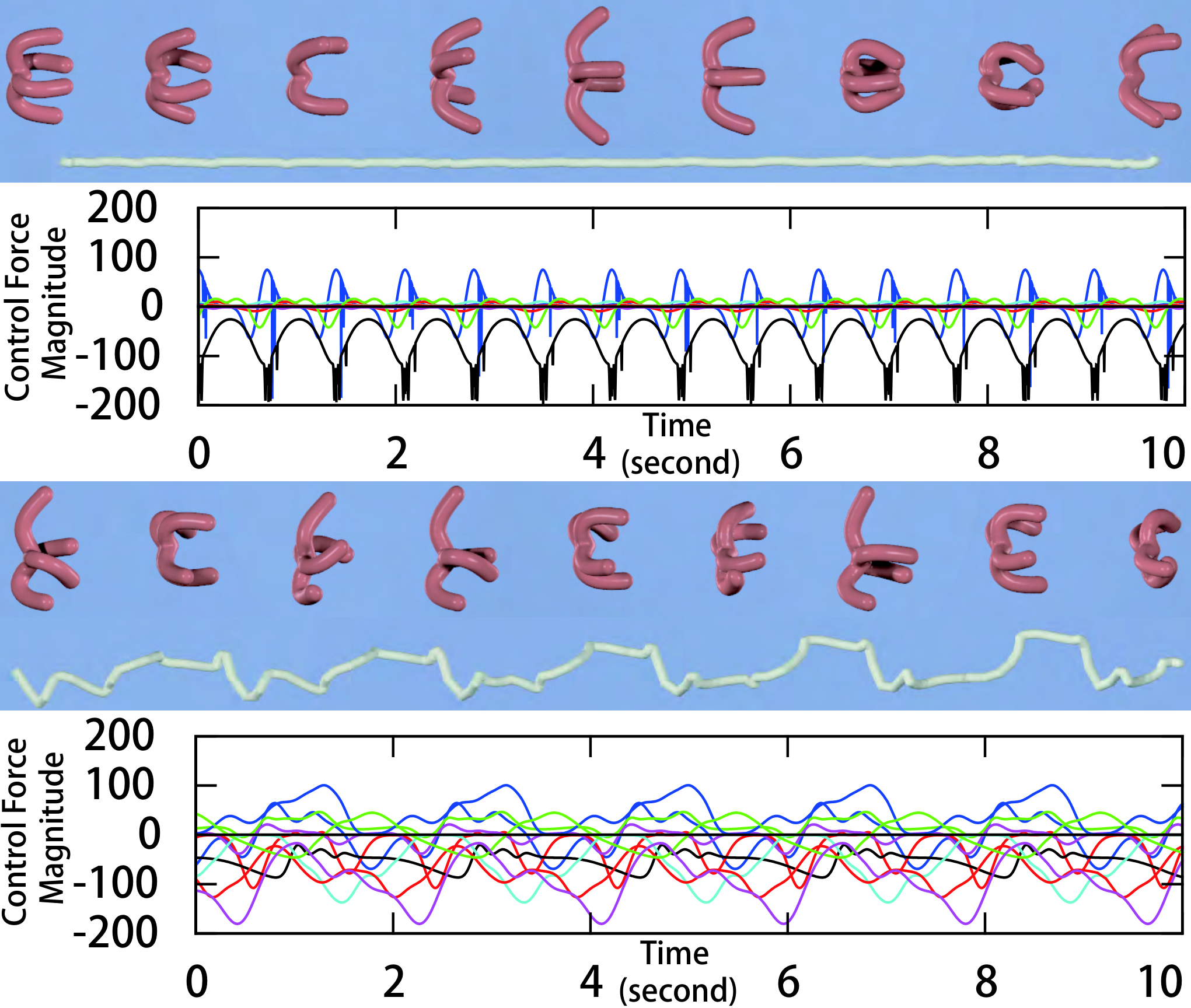
The approach highlighted above greatly increases the chances that our optimization algorithm computes a good local minima without significant computational overhead. This is because periodic DMP formulation (Equation 8) is guiding the whole trajectory to follow a same gait. When our optimization algorithm finds a useful gait, this information is quickly encoded into the DMP controller and reused to compute the entire trajectory using the formulation. In order to highlight this feature, we show two swimming trajectories computed using our optimization algorithm. In order to compute the trajectory shown in Figure 10 (a), we initialize the spider pose to at all timesteps. While to generate Figure 10 (b), we initialize the spider to a different random pose at every timestep. Moreover, the convergence history of these two optimization schemes are plotted in Figure 11. Our optimizer converges to two different but almost equally effective swimming gaits with very small objective function values. This means that although there are numerous local minima, most of them leads to plausible animations. However, bad local minima can still happen especially in contact-rich animations and we illustrate one such failure case in Figure 9.
6. Results
In this section, we highlight the results on complex benchmarks.
| Name | Value |
|---|---|
| dynamic | |
| Young’s modulus | |
| Poisson’s ratio | |
| Mass density | |
| Gravity | |
Parameter Choices: We use an identical set of parameters listed in Table 2 for all the benchmarks. The coefficient of the physics violation term is . Some parameters are related to , which is the average element size. If a deformable body has volume and is discretized using FEM elements, then . An exception is the coefficient for , which is adaptively adjusted within the optimization algorithm.
Benchmarks: We implemented our method in C++ and tested it on many benchmarks using a desktop machine with dual E5-2670 12-core CPU 2.1GHz and 12GB of memory. Given only a volumetric mesh and a definition of the environment, we first precompute the reduced dynamic model using [Pan et al., 2015]. We also precompute the surface cubatures to approximate the fluid drag forces. We use OpenMP to parallelize the function and gradient evaluations and run at most 10000 iterations of optimizations or stop early, if the relative error of is smaller than . The setup and computational cost in each benchmark is summarized in Table 3 and analyzed below.
| Example | Pre./PreSF.(min) | K/ | Opt.(hr) | App. | ||||
|---|---|---|---|---|---|---|---|---|
| Fish Swimming (Fig.12a) | 2118/7812 | 5 | 0.8/0.1 | 200/3 | 1.7 | DMP | ||
| Spider Swimming (Fig.12b) | 1054/4033 | 10 | 1.2/0.3 | 200/3 | 2.5 | DMP | ||
|
1054/4033 | 65 | 4.6/0.3 | 200/1 | 3.9 | None | ||
| Spider Walking (Fig.13) | 1054/4033 | 10 | 1.2/ | 200/4 | 5.2 | FB | ||
| Dragon Walking (Fig.7) | 929/1854 | 10 | 1.3/ | 200/1 | 2.2 | None | ||
| Letter T Walking (Fig.19a) | 1523/3042 | 15 | 1.1/ | 200/4 | 4.5 | FB | ||
|
1523/3042 | 65 | 4.2/ | 200/1 | 3.1 | None | ||
| Beam Jumping (Fig.14) | 1024/640 | 10 | 1.1/ | 100/1 | 1.1 | None | ||
| Cross Rolling (Fig.16) | 623/1499 | 10 | 1.3/ | 200/1 | 2.1 | None | ||
| Dinosaur Walking (Fig.18) | 1493/5249 | 15 | 0.9/ | 200/1 | 1.9 | None |
Fish Swimming: Fishes have the simplest deformable bodies and can be used for testing the performance of our method. As illustrated in Figure 1, a fish swims by simply swinging its body, so we use a reduced configuration space of small DOFs: , i.e., . Under this setting, we command the fish to swim straight forward in a gravityless environment using the following objective:
| (12) |
where transforms the velocity to a global frame of reference and is the target swimming speed in a local frame of reference. In addition, we add a balance energy to encourage fixed orientation:
| (13) |
where is the balance direction. Here we use , the unit gravitational direction. We can even navigate the fish to an arbitrary 3D point by optimizing 3 trajectories: swimming forward, swimming left, and swimming right. For swimming left and right, we add the following objective functions in addition to Equation 12:
| (14) |
where is the target rotating speed, we use again. After the optimization, the DMP function can be used as an open-loop controller to generate controlled forward simulations at real-time framerate. In Figure 12 (a), we wrap our forward simulator into a sampling-based motion planner, RRT* [Karaman and Frazzoli, 2011], to navigate the fish to look for food plants.

Spider Swimming: We also evaluated our approach on a more complex model: a four-legged spider. More degrees of freedom are used to allow each leg to move independently, so we use more DOFs: , i.e., . Again, we optimize to generate 3 trajectories with the same and for all trajectories. However, for the first trajectory we set , and for the other two we set so that the spider cannot turn itself around while swimming forward. This gives very different gaits for turning and swimming forward. We again use DMP to drive the realtime forward simulator and wrap it into a motion planner, as illustrated in Figure 12 (b).
Spider Walking: To analyze the walking animation, we use the same spider model and objective Equation 12 but replace the fluid drag force model with the frictional contact force model. However, we observe that this optimization takes approximately twice as many iterations to converge due to the contact-integrity term and the shuffle avoidance term . In Figure 13, we illustrate the walking gaits for two kinds of environments.

Similar to swimming, we allow a user to navigate the spider on the ground by optimizing 4 trajectories: walking left, right, backward, and forward, where the objective function is Equation 14 with corresponding . We then use a feedback controller similar to [Tan et al., 2012] to drive forward simulator. Specifically, we optimize over one timestep () with the objective function:
| (15) |
where is the configuration of the tracked trajectory. Due to the efficiency of reduced representation, such short-horizon optimization can be solved at realtime framerates.
Letter T Walking: A more challenging example is Letter T walking, as illustrated in Figure 6. This model has no static stability, so it must keep jumping to move around. Again, we first optimize 4 trajectories and then track these trajectories at realtime to navigate the character.
Beam Jumping: Jumping is an essential component in many animations. To generate these animations, we use the following objective function:
| (16) | |||
where the first term specifies the target altitude and the second term specifies the target horizontal velocity so that the character can jump forward. Using different and , we generate a series of results in Figure 14 and Figure 15 for a small beam, where the beam exhibits huge and varied deformations.


Cross Rolling: As illustrated in Figure 16 (b), we generate a rolling animation for a cross-shaped deformable body using the objective function Equation 13 and Equation 14. In addition, we notice that the deformable body in this example is close to planar. Therefore, we generated a second animation by restricting all the deformations to the 2D plane. As shown in Figure 16 (c), the deformable body exhibits very different gaits in this case. Also, this result shows that our hybrid optimization algorithm can automatically compute a very different mean pose (a swastika) from the rest pose (an X) in order to perform the locomotion task in an energy-efficient manner.


6.1. Combining our Algorithm with Partial Keyframe Data
Although our main contribution is a control framework that does not require keyframes, we can easily take keyframes into consideration to provide more flexibility to a user. These keyframes can either be specified fully or partially. A full keyframe specifies a target position for each of the vertices, while a partial keyframe only specifies a target position for a subset of vertices on the deformable body. For example, in Figure 18 (a), we show a dinosaur walking on the ground with its head swinging periodically to the left and right. The dinosaur’s head is guided by a set of partial keyframes illustrated in Figure 18 (b). The keyframes only specify the head and torso poses and we leave the leg poses to be determined by other objective function terms. We denote these keyframes as specified at timesteps . Note that these keyframes only specify the dinosaur’s deformable poses and do not affect the global transformation . The keyframe guiding is achieved using an additional objective function:
| (17) |
where is an importance-weighting matrix allowing the users to specify partial keyframes. In our example, is a diagonal matrix with diagonal value around the head and torso ( vertices) and elsewhere.

6.2. Analysis
We summarize objective functions used in all benchmarks in Table 4 and analyze several aspects of our method.
| Example | |
|---|---|
| Fish Swimming | |
| Spider Swimming | |
| or | |
| Walking | |
| Dinosaur Walking | |
| Jumping | |
| Rolling | |
| and |
Two-Stage Algorithm: A drawback of our method is that the optimization formulation takes a more complex form, and the resulting optimization algorithm takes longer time than [Barbič et al., 2009]. Fortunately, the DMP function returned by the optimizer can be used as a swimming controller to generate more swimming animation at realtime, as illustrated in Figure 12. This makes our method much more useful than a simple keyframe interpolation. However, to generate realtime contact-rich animations, such as walking and jumping, we have to use a feedback controller instead of DMP controller. This is because the contact forces are very sensitive to the discrepancy between forward simulation model and the physics model used in spacetime optimization (model discrepancy).
Multi-Tasking: In order to make the realtime animations directable, we need to simultaneously optimize multiple animation trajectories to allow a motion planner to pick trajectory online. However, if we sequentially run separate optimizations, the generated gaits can be quite different, e.g., the fish might swing its body with different frequencies to swim in different directions. This artifact can be mitigated if we use the same DMP parameters and for all the trajectories to ensure the same period of movement and phase shift, i.e., DMPs differ only in and for different tasks. This idea has been previously used for DMP-based reinforcement learning [Rückert and D’Avella, 2013]. As illustrated in Figure 17, DMP can represent large gait differences using different and only, while the rhythms of the movements are synchronized. We use this strategy in all the navigation examples.
Quality Measure: For jumping animation, we do not require any manual bases design such as basis expansion [Tan et al., 2012]. The reason is that we formulated physics constraints as soft constraints and physics constraints are violated for small tracking errors. To measure the violation to EOM at each frame , we first solve Equation 4 using to find a physically correct . Next, we measure the relative error against the average element size in Euclidean space using:
According to the plot in Figure 19, the physics violation over the whole trajectory is always less then half of average element size and is neglectible. The physics violation data for other examples can be found in Appendix D . However, manual bases design can sometimes be needed. For example, very different rolling gaits are generated in Figure 16, by restricting the bases to the 2D plane.

Effect of Different Parameters: Instead of using keyframes, the result of our algorithm depends on two sets of parameters. A first set of parameters are listed in Table 2. These parameters are considered internal and not exposed to users. The second set of parameters listed in Table 4 are exposed to users. These parameters have clear meanings such as walking, swimming, or rolling speed. In Figure 20, we highlight the effectiveness of performing animation control using the parameters listed in Table 4. We generated 9 walking/swimming trajectories using different target moving speed . Since we model as a soft penalty, the desired speed cannot be achieved exactly. However, according to Figure 20, the discrepancy between actual and desired moving speeds are very small. Therefore, we expose more parameters to the users compared with keyframe-based methods [Barbič et al., 2009; Schulz et al., 2014], these parameters have intuitive meanings and are helpful for animation control.
We also noticed two cases from Figure 20 (green circles) where the discrepancy between desired and actual moving speed are relatively large. If the desired speed is too small, then our optimizer considers as unimportant and it is given lower importance in order to reduce the residue in other objective terms. If the desired speed is too large, it can result in self-collisions or the optimizer falls into a bad local minima, as shown in Figure 9.
External vs. Internal Control Forces: Theoretically, our algorithm only uses internal forces to control the deformable body because our control force is dot-producted only with , instead of the entire in Equation 4. Therefore, it does not change the global translation and rotation . However, since we formulate the physical correctness as a penalty term, , rather than a hard constraint, there is some residual at the local minima. This residual can be interpreted as a violation of the physical correctness, or as a ghost external force. If we write , we are actually controlling the deformable body using both internal force and an additional ghost external force , but our objective function is designed to guide the optimizer to search for a solution with minimal ghost external force magnitude.
Using soft penalty instead of hard constraints also allows us to generate realtime deformable body animations by tracking an optimized animation. For example, having the letter-T balanced on a single contact point in Figure 19 is very challenging, which usually requires control over long horizons. However, with soft penalty, we can track the animation by control over only one timestep using Equation 15 as the objective function.
Robustness of Reduced Model Construction: A critical step in our method is the construction of the reduced model. Although this procedure takes several parameters, prior work [An et al., 2008; Pan et al., 2015] have resulted in robust algorithms that perform consistently well on a large dataset using same parameters. Therefore, we consider the construction of reduced model fully automatic. For example, to select the set of surface patches in Equation 11 and to construct the transformation function , we use cubature optimization. This procedure requires a training dataset. Our dataset is constructed by sampling 1000 Gauss-distributed deformable body poses as suggested in [An et al., 2008]. In order to solve the dictionary learning for the set of cubatures ( in Equation 11), we use L0-optimization proposed in [Pan et al., 2015] which automatically determine the required number of cubatures. We follow [Pan et al., 2015] in all other parameter settings and have never observed any failure cases.
Other Reduced Models: Although we choose [Pan et al., 2015], our method can also work with other reduced models. This can be done by modifying the transformation function and the kinetic energy in Equation 4. In Appendix C, we analyze the case with two kinds of different but widely used reduced models: LMA [Pentland and Williams, 1989] and reduced StVK [Barbič and James, 2005]. And two examples are illustrated in Figure 21 (a,b).
A drawback of these alternative models is that they require a higher-dimensional configuration space to achieve similar results as [Pan et al., 2015]. In our experiments, we use and each optimization becomes 3-5 times slower according to Table 1. However, from the plots of DMP control force magnitudes, Figure 21 (c,d), we notice that the optimal is actually very sparse. In other words, much computations are wasted on looking for small, unimportant control forces. Such analysis suggests that [Pan et al., 2015] is a better choice.
Although our formulation can also work with fullspace deformable models by replacing with identity function, this approach can be computationally very expensive. As reported in [Pan et al., 2015], using a reduced model accelerates the evaluation of by two orders of magnitude. In our experiments, cubature accelerates the evaluation of fluid drag forces by at least an order of magnitude using Equation 11. Since function evaluation is the major bottleneck of spacetime optimization, we expect it will take weeks or even months to finish an optimization using fullspace models. As a result, it is important to use reduced deformable models for efficiency reasons.

7. Limitations and Future Work
We present a method to automatically generate active animations of reduced deformable bodies, where the user provides a high-level objective and the animation is generated automatically using spacetime optimization. We take into account physics constraints, environmental forces in terms of CIO and fluid drag models, and DMP-based controller parametrization, so that the local minima of our objective function corresponds to a plausible animation. By evaluating objective functions and function gradients in a subspace, the optimization can be accomplished within several hours on a single desktop machine. Although optimization is offline, the results can be used to generate animations at realtime rates. For swimming animations, the optimized DMPs can be used as a controller for forward simulation. Unfortunately, DMP cannot be used as controllers for contact-rich animations. Since DMP is not a feedback controller, model discrepancy can quickly accumulate, leading to failures such as falling. In these cases, DMP is just used as a periodic and smoothness prior.
Our approach has some limitations. First, our method inherits all the limitations of the underlying reduced model. For example, current reduced model [Pan et al., 2015] cannot work with user specified skeletons. Working with skeletons is a desirable feature in terms of modelling some animal-like deformable bodies, such as the fish, where deformable tissues are covering skeletal bones. In addition, although our method requires no keyframes or user designs, we still ask the users to choose the form of and their parameters in Section 6. And without keyframes, the animations may not exhibit the same level of naturalness as some prior keyframe-based methods [Barbič et al., 2009]. Moreover, our optimizer may get stuck in a bad local minima due to insufficient DOFs of the reduced configuration space, a sub-optimal bases set, or an inappropriate settings of the weights. Furthermore, the inherent limitations of CIO term [Mordatch et al., 2013] for contact modeling and the fluid drag model can also affect our results. For example, we cannot have a deformable body bouncing off the ground since the CIO term only models inelastic contacts. CIO also allows inexact contacts to occur anywhere in the air, not only on the ground. Finally, like all the optimization-based motion planners, the performance of our method is still governed by a large set of parameters. Some parameters, such as the number of DMPs , are determined empirically. We have not evaluated the sensitivity of our method with respect to these parameters.
There are avenues for future work. First, incorporating some body-specific priors can be helpful in several ways. For example, for many muscle-driven deformable bodies, the user might want to parameterize the controller using muscle-tendon units [Wang et al., 2012] to generate more life-like animations. Another part that may benefit from user interactions is the identification of deformation bases in Figure 2. Currently, we identify these components using standard techniques [Pan et al., 2015] that are designed for visual simulation. However, it is not known if a base set for plausible visual simulation is suitable for character locomotion. It is also attractive to consider the optimization method as a general feedback controller, instead of an open-loop controller, for reduced deformable models using reinforcement learning [Peng et al., 2017]. Finally, developing control methods for two-way couple deformable body and articulated body will provide more flexibility to users. A starting point can be [Xu and Barbič, 2016].
References
- An et al. [2008] Steven S. An, Theodore Kim, and Doug L. James. 2008. Optimizing Cubature for Efficient Integration of Subspace Deformations. In ACM SIGGRAPH Asia 2008 Papers (SIGGRAPH Asia ’08). ACM, New York, NY, USA, Article 165, 10 pages. https://doi.org/10.1145/1457515.1409118
- Barbič et al. [2009] Jernej Barbič, Marco da Silva, and Jovan Popović. 2009. Deformable Object Animation Using Reduced Optimal Control. In ACM SIGGRAPH 2009 Papers (SIGGRAPH ’09). ACM, New York, NY, USA, Article 53, 9 pages. https://doi.org/10.1145/1576246.1531359
- Barbič and James [2005] Jernej Barbič and Doug L. James. 2005. Real-Time Subspace Integration for St. Venant-Kirchhoff Deformable Models. In ACM SIGGRAPH 2005 Papers (SIGGRAPH ’05). ACM, New York, NY, USA, 982–990. https://doi.org/10.1145/1186822.1073300
- Barbič and James [2010] Jernej Barbič and Doug L. James. 2010. Subspace Self-collision Culling. ACM Trans. Graph. 29, 4, Article 81 (July 2010), 9 pages. https://doi.org/10.1145/1778765.1778818
- Barbič et al. [2012] Jernej Barbič, Funshing Sin, and Eitan Grinspun. 2012. Interactive Editing of Deformable Simulations. ACM Trans. Graph. 31, 4, Article 70 (July 2012), 8 pages. https://doi.org/10.1145/2185520.2185566
- Barbič and Zhao [2011] Jernej Barbič and Yili Zhao. 2011. Real-time Large-deformation Substructuring. In ACM SIGGRAPH 2011 Papers (SIGGRAPH ’11). ACM, New York, NY, USA, Article 91, 8 pages. https://doi.org/10.1145/1964921.1964986
- Bergou et al. [2007] Miklós Bergou, Saurabh Mathur, Max Wardetzky, and Eitan Grinspun. 2007. TRACKS: Toward Directable Thin Shells. In ACM SIGGRAPH 2007 Papers (SIGGRAPH ’07). ACM, New York, NY, USA, Article 50. https://doi.org/10.1145/1275808.1276439
- Boyd et al. [2011] Stephen Boyd, Neal Parikh, Eric Chu, Borja Peleato, and Jonathan Eckstein. 2011. Distributed Optimization and Statistical Learning via the Alternating Direction Method of Multipliers. Found. Trends Mach. Learn. 3, 1 (Jan. 2011), 1–122. https://doi.org/10.1561/2200000016
- Bridson et al. [2002] Robert Bridson, Ronald Fedkiw, and John Anderson. 2002. Robust Treatment of Collisions, Contact and Friction for Cloth Animation. ACM Trans. Graph. 21, 3 (July 2002), 594–603. https://doi.org/10.1145/566654.566623
- Calakli and Taubin [2011] F. Calakli and G. Taubin. 2011. SSD: Smooth Signed Distance Surface Reconstruction. Computer Graphics Forum 30, 7 (2011), 1993–2002. https://doi.org/10.1111/j.1467-8659.2011.02058.x
- Capell et al. [2002] Steve Capell, Seth Green, Brian Curless, Tom Duchamp, and Zoran Popović. 2002. Interactive Skeleton-driven Dynamic Deformations. In Proceedings of the 29th Annual Conference on Computer Graphics and Interactive Techniques (SIGGRAPH ’02). ACM, New York, NY, USA, 586–593. https://doi.org/10.1145/566570.566622
- Chentanez et al. [2009] Nuttapong Chentanez, Ron Alterovitz, Daniel Ritchie, Lita Cho, Kris K. Hauser, Ken Goldberg, Jonathan R. Shewchuk, and James F. O’Brien. 2009. Interactive Simulation of Surgical Needle Insertion and Steering. In ACM SIGGRAPH 2009 Papers (SIGGRAPH ’09). ACM, New York, NY, USA, Article 88, 10 pages. https://doi.org/10.1145/1576246.1531394
- Choi and Ko [2005] Min Gyu Choi and Hyeong-Seok Ko. 2005. Modal warping: real-time simulation of large rotational deformation and manipulation. IEEE Transactions on Visualization and Computer Graphics 11, 1 (Jan 2005), 91–101. https://doi.org/10.1109/TVCG.2005.13
- Coros et al. [2012] Stelian Coros, Sebastian Martin, Bernhard Thomaszewski, Christian Schumacher, Robert Sumner, and Markus Gross. 2012. Deformable Objects Alive! ACM Trans. Graph. 31, 4, Article 69 (July 2012), 9 pages. https://doi.org/10.1145/2185520.2185565
- Gallego and Yezzi [2015] Guillermo Gallego and Anthony Yezzi. 2015. A Compact Formula for the Derivative of a 3-D Rotation in Exponential Coordinates. Journal of Mathematical Imaging and Vision 51, 3 (March 2015), 378–384. https://doi.org/10.1007/s10851-014-0528-x
- Hahn et al. [2012] Fabian Hahn, Sebastian Martin, Bernhard Thomaszewski, Robert Sumner, Stelian Coros, and Markus Gross. 2012. Rig-space Physics. ACM Trans. Graph. 31, 4, Article 72 (July 2012), 8 pages. https://doi.org/10.1145/2185520.2185568
- Harmon and Zorin [2013] David Harmon and Denis Zorin. 2013. Subspace Integration with Local Deformations. ACM Trans. Graph. 32, 4, Article 107 (July 2013), 10 pages. https://doi.org/10.1145/2461912.2461922
- Hauser et al. [2003] Kris K. Hauser, Chen Shen, and James F. O’Brien. 2003. Interactive Deformation Using Modal Analysis with Constraints. In Graphics Interface. CIPS, Canadian Human-Computer Commnication Society, 247–256. http://graphics.cs.berkeley.edu/papers/Hauser-IDU-2003-06/
- Hildebrandt et al. [2012] Klaus Hildebrandt, Christian Schulz, Christoph von Tycowicz, and Konrad Polthier. 2012. Interactive Spacetime Control of Deformable Objects. ACM Trans. Graph. 31, 4, Article 71 (July 2012), 8 pages. https://doi.org/10.1145/2185520.2185567
- Irving et al. [2006] G. Irving, J. Teran, and R. Fedkiw. 2006. Tetrahedral and Hexahedral Invertible Finite Elements. Graph. Models 68, 2 (March 2006), 66–89. https://doi.org/10.1016/j.gmod.2005.03.007
- James and Pai [2004] Doug L. James and Dinesh K. Pai. 2004. BD-tree: Output-sensitive Collision Detection for Reduced Deformable Models. In ACM SIGGRAPH 2004 Papers (SIGGRAPH ’04). ACM, New York, NY, USA, 393–398. https://doi.org/10.1145/1186562.1015735
- Karaman and Frazzoli [2011] Sertac Karaman and Emilio Frazzoli. 2011. Sampling-based algorithms for optimal motion planning. The International Journal of Robotics Research 30, 7 (2011), 846–894. https://doi.org/10.1177/0278364911406761 arXiv:http://dx.doi.org/10.1177/0278364911406761
- Kim and Pollard [2011] Junggon Kim and Nancy S. Pollard. 2011. Fast Simulation of Skeleton-driven Deformable Body Characters. ACM Trans. Graph. 30, 5, Article 121 (Oct. 2011), 19 pages. https://doi.org/10.1145/2019627.2019640
- Kim and James [2011] Theodore Kim and Doug L. James. 2011. Physics-based Character Skinning Using Multi-domain Subspace Deformations. In Proceedings of the 2011 ACM SIGGRAPH/Eurographics Symposium on Computer Animation (SCA ’11). ACM, New York, NY, USA, 63–72. https://doi.org/10.1145/2019406.2019415
- Liu and Nocedal [1989] Dong C. Liu and Jorge Nocedal. 1989. On the limited memory BFGS method for large scale optimization. Mathematical Programming 45, 1 (1989), 503–528. https://doi.org/10.1007/BF01589116
- Liu et al. [2013] Libin Liu, KangKang Yin, Bin Wang, and Baining Guo. 2013. Simulation and Control of Skeleton-driven Soft Body Characters. ACM Trans. Graph. 32, 6, Article 215 (Nov. 2013), 8 pages. https://doi.org/10.1145/2508363.2508427
- Lourakis [2005] Manolis IA Lourakis. 2005. A brief description of the Levenberg-Marquardt algorithm implemented by levmar. (2005).
- Mordatch et al. [2012] Igor Mordatch, Emanuel Todorov, and Zoran Popović. 2012. Discovery of Complex Behaviors Through Contact-invariant Optimization. ACM Trans. Graph. 31, 4, Article 43 (July 2012), 8 pages. https://doi.org/10.1145/2185520.2185539
- Mordatch et al. [2013] Igor Mordatch, Jack M. Wang, Emanuel Todorov, and Vladlen Koltun. 2013. Animating Human Lower Limbs Using Contact-invariant Optimization. ACM Trans. Graph. 32, 6, Article 203 (Nov. 2013), 8 pages. https://doi.org/10.1145/2508363.2508365
- Mukadam et al. [2016] M. Mukadam, X. Yan, and B. Boots. 2016. Gaussian Process Motion planning. In 2016 IEEE International Conference on Robotics and Automation (ICRA). 9–15. https://doi.org/10.1109/ICRA.2016.7487091
- Müller and Gross [2004] Matthias Müller and Markus Gross. 2004. Interactive Virtual Materials. In Proceedings of Graphics Interface 2004 (GI ’04). Canadian Human-Computer Communications Society, School of Computer Science, University of Waterloo, Waterloo, Ontario, Canada, 239–246. http://dl.acm.org/citation.cfm?id=1006058.1006087
- Pan et al. [2015] Zherong Pan, Hujun Bao, and Jin Huang. 2015. Subspace Dynamic Simulation Using Rotation-strain Coordinates. ACM Trans. Graph. 34, 6, Article 242 (Oct. 2015), 12 pages. https://doi.org/10.1145/2816795.2818090
- Peng et al. [2017] Xue Bin Peng, Glen Berseth, Kangkang Yin, and Michiel Van De Panne. 2017. DeepLoco: Dynamic Locomotion Skills Using Hierarchical Deep Reinforcement Learning. ACM Trans. Graph. 36, 4, Article 41 (July 2017), 13 pages. https://doi.org/10.1145/3072959.3073602
- Pentland and Williams [1989] A. Pentland and J. Williams. 1989. Good Vibrations: Modal Dynamics for Graphics and Animation. SIGGRAPH Comput. Graph. 23, 3 (July 1989), 207–214. https://doi.org/10.1145/74334.74355
- Rückert and D’Avella [2013] Elmar Rückert and Andrea D’Avella. 2013. Learned parametrized dynamic movement primitives with shared synergies for controlling robotic and musculoskeletal systems. Frontiers in Computational Neuroscience 7 (2013), 138. https://doi.org/10.3389/fncom.2013.00138
- Schaal [2006] Stefan Schaal. 2006. Dynamic movement primitives-a framework for motor control in humans and humanoid robotics. In Adaptive motion of animals and machines. Springer, 261–280.
- Schulz et al. [2014] Christian Schulz, Christoph von Tycowicz, Hans-Peter Seidel, and Klaus Hildebrandt. 2014. Animating Deformable Objects Using Sparse Spacetime Constraints. ACM Trans. Graph. 33, 4, Article 109 (July 2014), 10 pages. https://doi.org/10.1145/2601097.2601156
- Tan et al. [2012] Jie Tan, Greg Turk, and C. Karen Liu. 2012. Soft Body Locomotion. ACM Trans. Graph. 31, 4, Article 26 (July 2012), 11 pages. https://doi.org/10.1145/2185520.2185522
- Terzopoulos et al. [1987] Demetri Terzopoulos, John Platt, Alan Barr, and Kurt Fleischer. 1987. Elastically Deformable Models. In Proceedings of the 14th Annual Conference on Computer Graphics and Interactive Techniques (SIGGRAPH ’87). ACM, New York, NY, USA, 205–214. https://doi.org/10.1145/37401.37427
- Todorov [2011] E. Todorov. 2011. A convex, smooth and invertible contact model for trajectory optimization. In 2011 IEEE International Conference on Robotics and Automation. 1071–1076. https://doi.org/10.1109/ICRA.2011.5979814
- Wang et al. [2012] Jack M. Wang, Samuel R. Hamner, Scott L. Delp, and Vladlen Koltun. 2012. Optimizing Locomotion Controllers Using Biologically-based Actuators and Objectives. ACM Trans. Graph. 31, 4, Article 25 (July 2012), 11 pages. https://doi.org/10.1145/2185520.2185521
- Witkin and Kass [1988] Andrew Witkin and Michael Kass. 1988. Spacetime Constraints. In Proceedings of the 15th Annual Conference on Computer Graphics and Interactive Techniques (SIGGRAPH ’88). ACM, New York, NY, USA, 159–168. https://doi.org/10.1145/54852.378507
- Xu and Barbič [2016] Hongyi Xu and Jernej Barbič. 2016. Pose-space Subspace Dynamics. ACM Trans. Graph. 35, 4, Article 35 (July 2016), 14 pages. https://doi.org/10.1145/2897824.2925916
- Yuksel et al. [2007] Cem Yuksel, Donald H. House, and John Keyser. 2007. Wave Particles. In ACM SIGGRAPH 2007 Papers (SIGGRAPH ’07). ACM, New York, NY, USA, Article 99. https://doi.org/10.1145/1275808.1276501
Appendix A Optimization Algorithm
In this section we summarize our main Algorithm 2. The skeleton of this algorithm is an LM optimizer. We refer readers to [Lourakis, 2005] for a brief introduction of this simple method. In our experiments, LM performs much better than LBFGS for two reasons. First, LM uses approximation of the hessian which usually leads to a better step size estimation. Second, although LM needs to search for the so-called damping coefficient as in the process of the line-search scheme, it requires only function value evaluations which are much faster than gradient evaluations used by the line-search scheme of LBFGS.
However, a minor problem with using an LM algorithm is that it assumes the objective function is a sum of squares, which is violated by . In Appendix A.1, we show that a marginal modification to [Lourakis, 2005] will allow us to handle .
After every successful LM iteration, we update ; we update every 10 iterations. Since each update leads to an energy value decrease, the algorithm is guaranteed to converge eventually. Finally, we also update the active vertices contributing to and in Line 32. A minor bottleneck in this algorithm is the sparse linear system in Line 8, but we notice that the hessian of is a block-tridiagonal matrix that can be inverted with linear time complexity.
A.1. LM Modification for
Conventional LM assumes that the objective function takes the form of where is a vector of nonlinear terms. This is not the case with . However, among the many implementations of LM, the one documented in [Lourakis, 2005] is not limited to the above form. If we have a certain approximation of the hessian of denoted as (not necessarily in the form of ) and use damping coefficient , then the update to in our main algorithm is computed as:
and the decrease in after applying the update is:
which is exactly the expected function value decrease estimation used in [Lourakis, 2005]. This allows us to use a non- form of approximate hessian for . In our case, we approximate the term by first order expansion for both and , giving:
and use the hessian of the last equation above. Conventional approximation of the hessian is used for all other terms.
A.2. Eliminating Internal Force Terms
In our objective function, is a quadratic function in , in the Tikhonov regularization , and in the DMP regularization . We analytically solve and eliminate from the optimization as follows:
Appendix B and its Derivatives
In this section, we briefly summarize the transformation function from the reduced representation to a vertex ’s Euclidean coordinates as defined in [Pan et al., 2015]. We then provide some guidance on the computation of and . Since we use the LM algorithm for space-time optimization, most objective terms only require a first order derivative . An exception is the physics violation term , which requires second order derivatives.
B.1. Transformation Function
We assume that a deformable body is discretized using vertices and elements. For each element , its deformation gradient is denoted as . Vertices’ Euclidean coordinates can be reconstructed from through Poisson reconstruction. We abbreviate this linear operator as:
It is well-known that above has a polar decomposition where is a rotation and is an anisotropic scaling. We can then use the Rodrigues formula on the rotation part to get , where is the rotation vector of element . The rotation-strain (RS) space is defined by the space spanned by all possible and :
RS representation and Euclidean coordinates are equivalent. However, using RS representation is advantageous because the most visually salient deformations lie in a low-dimensional linear subspace of . Therefore, we can use conventional linear dimensionality reduction techniques such as linear modal analysis [Pentland and Williams, 1989] in RS space to arrive at the following low-rank approximation:
where is a set of bases in the RS subspace. The transformation function from to can then be defined by combining the above equations:
However, this only encodes deformations in the local frame of reference. To allow arbitrary movement in the global frame of reference, we can superimpose a global translation and rotation , giving:
B.2. Kinetic Cubature Acceleration
Merely having the low-rank approximation does not accelerate computation. The evaluation of is still computationally costly because it requires a summation over all the elements. This procedure can be accelerated using cubature approximation by assuming the following approximation:
where is the block of corresponding to the th element. The weighting and the set of cubature elements are precomputed using L0-optimization.
B.3. Derivatives
To derive and , we notice that they can always be written as a long chain of matrix productions, where each matrix is either a constant, a linear function of , or a linear function of , , and . Equations of this form can be accelerated using fast sandwich transform (FST) [Kim and James, 2011], i.e., by precomputing high-order tensors and contracting them with , , and at runtime. The remaining problem is to derive and . A closed-form of can be found in [Gallego and Yezzi, 2015]. We now derive below using their notations:
where we used the identity , , , and . Finally, the above has the following form:
Appendix C Other Reduced Models
In this section, we analyze the cases where rotation-strain coordinates [Pan et al., 2015] is replaced with either LMA [Pentland and Williams, 1989] or reduced StVK [Barbič and James, 2005]. As mentioned in Section 6.2, we need to modify both and in Equation 4. In both cases, takes the following simple form:
where is a set of linear deformation bases. Due to the lack of rotation-strain transformation, we have to introduce more columns to than in order to represent nonlinear deformations. If LMA is used, takes the same quadratic form as that for rotation-strain coordinates, . If reduced StVK is used, is a quartic function in whose polynomial coefficients can be precomputed.
Appendix D Physics Violation
We provide the physics violation data for all the examples in Table 6. We use the same criterion:
Compared with the average FEM element size , the error due to physics violation is very small. The parameters for all the volumetric deformable models are provided in Table 5.
| Model | l | |
|---|---|---|
| Fish | ||
| Spider | ||
| Letter T | ||
| Dragon | ||
| Beam | ||
| Cross |
| Fish Swimming | Spider Swimming |
|---|---|
| Spider Walking | Letter T Walking |
| Dragon Walking | Beam Jumping |
| Cross Rolling | |