Capital flow constrained lot sizing problem with loss of goodwill and loan

We adopt the following notations for our model. Some relevant notations will be introduced when needed.

The decision variables used in the models include the following:
$B_{t}\hskip 10.00002pt$ end-of-period capital for period $t$. $I_{t}\hskip 10.00002pt$ end-of-period inventory level for period $t$. $x_{t}\hskip 10.00002pt$ a binary variable signaling whether the production occurs in period $t$. $y_{t}\hskip 10.00002pt$ production quantity in period $t$. $w_{t}\hskip 10.00002pt$ demand shortage (lost sales) in period $t$, and we define $w_{0}=0$. $Ed_{t}\hskip 10.00002pt$ effective demand in period $t$ when considering customer goodwill loss. $v_{t}\hskip 10.00002pt$ realized demand in period $t$ and $v_{t}=Ed_{t}-w_{t}$. $\delta_{t}\hskip 10.00002pt$ a binary variable signaling whether $Ed_{t}$ is positive.

In our problem, we make the following assumptions:

1. 1.

   Initial capital of period $t$ should not be less than the total production cost in period $t$, namely, $B_{t-1}\geq s_{t}x_{t}+c_{t}y_{t}$, in which initial capital of period $t$ is $B_{t-1}$, and the total production cost in period $t$ is production launching cost $s_{t}x_{t}$ plus variable production cost $c_{t}y_{t}$.

2. 2.

   End-of-period capital for each period should be not less than 0, namely, $B_{t}\geq 0$.

3. 3.

   Initial inventory of the planning horizon is 0, namely, $I_{0}=0$.

4. 4.

   No backorder is allowed.

5. 5.

   The manufacturer could decide the realized quantity for customer’s demand without paying penalty cost, but lost sales can cause the shrinking of demand in the next period.

6. 6.

   The manufacturer uses loan in the first period and pays back the principal and interest after a certain length of periods; length of loan is shorter than the length of total planning horizon; mortgages are not required for loan.

The biggest difference between our problem and traditional lot sizing problem is Assumption 1 and 2: how much to produce is constrained by present capital, and end-of-period capital for each period should be above zero to avoid bankruptcy. Assumption 3 and 4 are also the standard assumptions of the Wagner-Whitin model. Assumption 5 means the manufacturer can decide how much products they want to provide for customers. Assumption 6 defines the loan type in our paper. Loan length is smaller than the total planning horizon because lenders tend to have higher risks for longer loan length and they generally don’t provide loan out of the planning horizon in order to reduce risks.

Considering loss of customer goodwill, effective demand is the remnant demand after the goodwill loss from the original demand. As in Aksen (2007), the effective demand in period $t$ can be represented as:

Eq. (1) is a nonlinear equation. For convenience of computation, we bring several linear constraints to replace this nonlinear equation and construct the mixed integer programming model below.

Model P

The objective defined by Eq. (2) is to maximize the capital increment from the beginning of the planning horizon to the final period, where the realized sales in period $t$ are given by $Ed_{t}-w_{t}$, revenue in period $t$ is $p_{t}(Ed_{t}-w_{t})$, total cost in period $t$ is $h_{t}I_{t}+s_{t}x_{t}+c_{t}y_{t}$, or $h_{t}I_{t}+s_{t}x_{t}+c_{t}y_{t}+B_{L}(1+r)^{T_{L}}$ if period $t$ should pay back the loan.

Constraint (3) enforces setups with positive production in each period. Constraint (4) represents Assumption 1 and 2: initial capital in period $t$ should be not less than the total production cost in period $t$. It also ensures the non-negativity of $B_{t-1}$, which avoids bankruptcy. Constraint (5) ensures that any lost demand $w_{t}$ in period $t$ not exceed the effective demand of that period. Constraint (6) provides the inventory flow balance equation, and Constraints (7) and (8) define the capital flow balance.

Constraints (9)-(13) are the linear descriptions of Eq. (1). Among them, Constraints (9) and (10) ensure the binarity of $\delta_{t}$: if $d_{t}\leq\beta w_{t-1}$, $\delta_{t}=0$ and effective demand $Ed_{t}$ is also 0, else, $\delta_{t}=1$ and effective demand $Ed_{t}$ is positive; Constraint (11), (12) and (13) determine the value of effective demand $Ed_{t}$: if $d_{t}\leq\beta w_{t-1}$, $\delta_{t}=0$ and $Ed_{t}=0$; else, $\delta_{t}=1$ and $Ed_{t}=d_{t}-\beta w_{t-1}$. Constraints (14), (15) and (16) guarantee the non-negativity and binarity of variables. Constraint (14) also represents Assumption 3 and 4 in our problem.

Note that if $\beta=0$, this model is transformed to a capital flow constrained problem without loss of goodwill.

The single-item capacitated lot sizing problem has been shown by Bitran and Yanasse (1982) to be NP-hard. As for our problem, the capital flow constraint $c_{t}y_{t}+s_{t}x_{t}\leq B_{t-1}$ is a capacity constraint by removing $s_{t}x_{t}$ and replacing $B_{t-1}$ with $C_{t}$, where $C_{t}$ is the capacity in period $t$. Therefore, capital flow constraint is a special type of capacity constraints, and model P is also a NP-hard problem.

Lemma 1 is apparently true when $t+1=1$ because $I_{0}=0$. For $t+1>1$, if there is a solution that does not satisfy Lemma 2, namely, $I_{t}>0$ and $y_{t+1}>0$, assume that period $t+1$’s former production cycle begins at period $m$ ($1\leq m\leq t$), and the production cycle beginning at period $t+1$ lasts till period $n$ ($n\leq T$). The production plan is shown in Figure 1.

According to capital flow balance equation (8), end-of-period capital for period $t$ and period $T$ are given by the following equations.

If the production quantity in period $m$ reduces $I_{t}$ and the production quantity in period $t+1$ increases $I_{t}$, then the effective demands $Ed_{i}$ ($i=1,\dots,T$) would not be influenced and the production plan is still feasible. $B_{t}$ and $B_{T}$ change to the following:

If unit variable production costs are equal, $B_{T}^{{}^{\prime}}=B_{T}+\sum\nolimits_{i=m}^{t}h_{i}I_{t}\geq B_{T}$, The final capital increases. Therefore, $I_{t}>0$ and $y_{t+1}>0$ is not the optimal solution; optimal solution always satisfies $I_{t}y_{t+1}=0$. ∎

Lemma 1 is also known as the zero-inventory-ordering policy, which means initial inventory of a production cycle is always zero. Define $f_{t}(I_{t-1},B_{t-1},w_{t-1})$ as the maximum capital increment during period $t,t+1,\dots,T$, given period $t$’s initial inventory $I_{t-1}$, initial capital $B_{t-1}$, and previous period’s demand shortage quantity $w_{t-1}$.

To prove this property, we build a dynamic programming model for our problem. For any at period $t$ ($t=1,\dots,T$), its states are: initial inventory $I_{t-1}$, initial capital is $B_{t-1}$, and demand shortage quantity of previous period $w_{t-1}$. Its actions are production quantity $y_{t}$ and demand realized quantity $v_{t}$. Lower bounds for $y_{t}$ and $v_{t}$ are both 0; Upper bound for $y_{t}$ is the maximum production quantity under present capital and upper bound for $v_{t}$ is the quantity of effective demand in this period, which are shown by Eq. (21) and Eq. (22), respectively.

Define a unit step function $K(z)$: $K(z)=1$ if $z>0$; $K(z)=0$ if $z\leq 0$. The state transition equations are:

The functional equation for dynamic programming is:

when $I_{t-1}$ and $w_{t-1}$ are fixed, if increasing $B_{t-1}$, from Eq. (21) and Eq. (22), the feasible domain for $v_{t}$ does not change, but the feasible domain for $y_{t}$ stays constant or expands. There always exists actions $y^{\prime}_{t}$ and $v^{\prime}_{t}$ that make $f^{\prime}_{t}(I_{t-1},B^{\prime}_{t-1},w_{t-1})$ not lower than $f_{t}(I_{t-1},B_{t-1},w_{t-1})$. Therefore, $f_{t}(I_{t-1},B_{t-1},w_{t-1})$ is nondecreasing with $B_{t-1}$ with fixed $I_{t-1}$ and $w_{t-1}$. ∎

The proof is similar to Lemma 2. If goodwill shortage rate is 0, demand shortage is not the states of the dynamic programming problem. The actions are still $y_{t}$ and $v_{t}$ and state transition equations are Eq. (23) and Eq. (24). The functional equation changes to be:

When $I_{t-1}$ are fixed and increasing $B_{t-1}$, feasible domain for $v_{t}$ keeps unchanged while feasible domain for $y_{t}$ stays constant or expands. Therefore, $f_{t}(I_{t-1},B_{t-1})$ is nondecreasing with $B_{t-1}$. ∎

Define $BB_{m,n}^{B_{m-1}}$ as the maximum capital increment in a production round from period $m$ to period $n$ with initial capital $B_{m-1}$. Based on Lemma 1, Lemma 2 and Lemma 3, our problem is approximately transformed to a traveling salesman problem finding the longest route as shown in Figure 2 (in this case, $T=4$). Main ideas behind this approximation are that we apply the zero-inventory-ordering policy to divide production plan into several production rounds, and apply Lemma 2 and Lemma 3 to always select maximum initial capital for computation of the length of arcs in the traveling salesman problem.

A functional equation is constructed for computation of the problem, and we set $B_{0}^{\ast}=B_{0}$.

Apparently, $B_{T}^{\ast}=\max\limits_{1\leq m\leq T}\left[B_{m-1}^{\ast}+BB_{m,T}^{B_{m-1}^{\ast}}\right]$. On this functional equation, we have the following properties.

If goodwill loss rate and end inventory level for period $t$ are both 0, based on Eq. (27), given initial capital and initial inventory, maximum capital increment during period $t$ to period $T$ is:

From Lemma 3, $f_{t+1}(0,B_{t})$ is a non-decreasing function of $B_{t}$, and gets the maximum value when $B_{t}$ is the maximum end-of-period capital for period $t$. Given zero end-of-period inventory in period $t$, this happens when the production plan from period 1 to $t$ is optimal because optimal production plan satisfies zero-inventory-ordering policy when the variable production costs are equal. So, what is optimal for period 1 to period $t$ is also optimal for $f_{t+1}(0,B_{t})$, which is the maximum capital increment during period $t+1$ to period $T$. Therefore, the optimal production plan from period 1 to $t$ is part of the optimal production plan from period 1 to $T$. ∎

By lemma 4, the optimal production plan from period 1 to $t_{1}-1$ is part of the whole production plan, and the optimal production plan from period 1 to $t_{1}-1$ is also part of the optimal production plan from period 1 to $t_{2}$. If the production plan from period $t_{1}$ to $t_{2}$ is optimal, together with the optimal plan form period 1 to $t_{1}-1$, it will result in an optimal production plan from period $1$ to $t_{2}$ under the zero-inventory-ordering policy. Since the optimal production plan from period 1 to $t_{2}$ is part of the whole production plan, the optimal production plan from period $t_{1}$ to $t_{2}$ is part of the optimal production plan from period 1 to $T$. ∎

When the variable production costs are equal, Lemma 1 shows the problem satisfies the zero-inventory ordering policy. Hence, the optimal production plan can be a combination of several production rounds. The functional equation (28) in fact enumerates all the possible production rounds. Lemma 4 and Lemma 5 indicate that the optimal production plan in a given production round is part of total optimal production plan. These are the same properties as the Wagner-Whitin case (Wagner and Whitin, 1958). Therefore, for all the combinations of production rounds in the computation of $B_{T}^{\ast}=\max\limits_{1\leq m\leq T}\left[B_{m-1}^{\ast}+BB_{m,T}\right]$, the one that gives maximum final capital is the optimal solution. ∎

When the variable production costs are not all equal, or goodwill loss rate is not 0, the functional equation in Theorem 1 only gets an approximate solution. However, based on some properties below, we devise some heuristic adjustments to make it close to the optimal solution.

The feasible solution is presented by Figure 4. For period $t_{3}+1$, its functional equation is

From Lemma 2, $f_{t_{3}+1}(I_{t_{3}},B_{t_{3}},w_{t_{3}})$ is non decreasing with $B_{t_{3}}$ when $I_{t_{3}}$ and $w_{t_{3}}$ are fixed. In the adjustment, $I_{t_{3}}$ are fixed to be 0, after increasing $B_{t_{3}}$ and decreasing $w_{t_{3}}$, the domains for $y_{t_{3}+1}$ and $v_{t_{3}+1}$ both expand from Eq. (21) and Eq. (22). Therefore, the final capital increment is non decreasing with this adjustment. ∎

The adjustment in Corollary 1 is shown by Figure 4.

This heuristic step is shown in Figure 5. If $B_{t_{1}-1}-s_{t_{1}}-c_{t_{1}}y_{t_{1}}>0$, production cycle $t_{1}$ has residual production capacity, which could produce more. After the moving adjustment, the final capital changes to the following:

If $c_{t_{1}}+\sum_{i=t_{1}}^{t_{2}-1}h_{i}<c_{t_{2}}$, this adjustment does not affect the feasibility of the solution and $B_{T}^{{}^{\prime}}>B_{T}$. Therefore, final capital increases. ∎

The moving production amount $\Delta y_{t_{2}}$ can be obtained by Eq. (32).

Eq. (32) is the maximum production quantity increment that cycle $t_{1}$ can provide.

By definition, $BB_{m,n}$ is the maximum capital increment in a production round. Therefore, it may include several production cycles. For a production round with fixed $k$ production cycles, assume the production launching periods are $t_{1}$, $t_{2}$, $\dots$, $t_{k}$ (for convenience of expression, we set $m=t_{1}$, $n=t_{k+1}-1$), the production plan is shown in Figure 6.

To compute $BB_{m,n}$, there are still integer variables $\delta_{t}$, which is a 0-1 variable indicating whether previous goodwill loss is below effective demand. In Model P-sub1 below, we use a heuristic step by assuming $\delta_{t}=1$, $m\leq t\leq n$, namely, all demand from period $m$ to period $n$ are above previous goodwill loss. With known $w_{t_{1}-1}$, we convert Model P to a sub linear problems P-sub1.

Model P-sub1

The objective function (33) is to maximize capital increment from a production round starting at period $m$ and ending at period $n$. Constraints (34) and (35) represents our paper’s assumptions 1 and 2 about capital flow constraints. Constraint (36) shows the relationship between $I_{t}$ and $v_{t}$. Constraint (37) and Constraint (38) are the capital flow balance. Constraint (39) means that initial inventory and end-of-period inventory of each production cycle are both zeros, which is a heuristic step if unit variable production costs are not equal. Constraints (40) and (41) are expressions of effective demands. Constraint (41) also reflects the heuristic assumption: $\delta_{t}=1$, $m\leq t\leq n$. Constraint (42) provides the lower and upper bounds of variables $v_{t}$, which is realized demand in period $t$.

If Model P-sub1 does not obtain a feasible solution, this may be related with the heuristic assumption of $\delta_{t}$. So next step we relax this assumption without loss of goodwill: removing Constraint (41) in Model P-sub1, amending Constraint (42) to get another sub linear problem P-sub2 below.

Model P-sub2

Based on the solution of Model P-sub2, compute $\delta_{t}$ according to equations (45) and (46) below.

Based on the values of $\delta_{t}$, another sub linear problem is formulated.

Model P-sub3

If Model P-sub1, Model P-sub2 and Model P-sub3 all do not have a feasible solution, we deem $BB_{m,n}$ does not have a feasible solution and set $v_{t}=0$ ($t=m,m+1,\dots,n$). The relation of $v_{t}$ with $w_{t}$ is provided by Eq. (45). The relation of $v_{t}$ with $y_{t}$ is given by Eq. (50).

It is time consuming and complex to enumerate all the possible production cycles in a production round. Therefore, when customer goodwill loss rate is zero, we use one production cycle in a production round; when goodwill loss rate is not zero, we use at most two production cycles in a production round for computation. For a certain period $t+1$ and given production plan from period 1 to period $t$, two situations are considered in computation of capital increment during a production round when goodwill loss rate is not zero: if there exists no production cycle before $t+1$, we compute only one production cycle beginning with period $t+1$ as a production round; if there exists production cycles before $t+1$, we view the nearest previous production cycle and the production cycle beginning with $t+1$ together as a production round, and make computations.

After computation of capital increments during production rounds, we can get an approximated production plan from period 1 to any period $n$ ($1\leq n\leq T$). Based on Corollary 1, we make heuristic adjustments to this production plan. Three situations are considered for this adjustment, which are shown by Figure 7. In Figure 7, period $n$’s production cycle beginning at period $t+1$.

• •

  Figure 7(a) means we make adjustments to the first production cycle in the production round $m$ to $n$: dividing the first production cycle into two cycles by enumerating all new production launching periods between period $m$ to period $t$; recomputing $BB_{m,n}$, and selecting the one which gives maximum capital increment.

• •

  Figure 7(b) means sometimes it’s better to launch a new production cycle before period $t+1$ when there exists no production cycles before it: enumerating all new production launching period between period $1$ to period $t$ as $m$; recomputing $BB_{m,n}$ and selecting the optimal one.

• •

  Figure 7(c) means sometimes it’s better to launch production later if the first production cycle include period 1: enumerating all new production launching period between period $1$ to period $t$ as $m$; recomputing $BB_{m,n}$, and selecting the optimal one that can give maximum capital increment.

In computing $BB_{m,n}$ for the three heuristic adjustments, a new linear constraint is added to the sub-linear problems: $w_{n}^{\prime}\leq w_{n}$, which means demand shortage at period $n$ after the adjustment should be not higher than its original value before the adjustment.

If goodwill loss rate is zero, Corollary 1 is not necessary and there is no need for the adjustments above. After the recursion of $BB_{m,n}$ till the final period $T$, a production plan for the the whole planning horizon is obtained. Backward from period $T$ to period 1, check if it satisfies the criteria of Corollary 2 and make production adjustments.

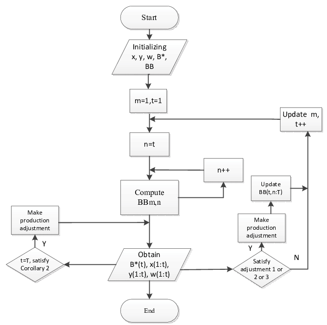
Based on functional equation (28), sub-linear problems and heuristic techniques, we propose a forward recursive algorithm with heuristic adjustment algorithm (FRH) to solve Model P.

Algorithm FRH for Model P

initialization:  $t=1$, $m=1$, $1\times T$ zero matrices $x$, $y$, $B^{\ast}$, $T\times T$ zero matrices $BB$.

References

- Absi et al (2013) Absi N, Detienne B and Dauzère-Pérès S (2013). Heuristics for the multi-item capacitated lot-sizing problem with lost sales. Computers & Operations Research 40(1):264–272.
- Aksen (2007) Aksen D (2007). Loss of customer goodwill in the uncapacitated lot-sizing problem. Computers & operations research 34(9):2805–2823.
- Aksen et al (2003) Aksen D, Altınkemer K and Chand S (2003). The single-item lot-sizing problem with immediate lost sales. European Journal of Operational Research 147(3):558–566.
- Berk et al (2008) Berk E, Toy AÖ and Hazır Ö (2008). Single item lot-sizing problem for a warm/cold process with immediate lost sales. European Journal of Operational Research 187(3):1251–1267.
- Bitran and Yanasse (1982) Bitran GR and Yanasse HH (1982). Computational complexity of the capacitated lot size problem. Management Science 28(10):1174–1186.
- Blazenko and Vandezande (2003) Blazenko GW and Vandezande K (2003). Corporate holding of finished goods inventories. Journal of Economics and Business 55(3):255–266.
- Bradley (2000) Bradley D (2000). Lack of financial and location planning causes small business bankruptcy. Ph.D. thesis, University of Central Arkansas, Conway, AR.
- Brahimi et al (2017) Brahimi N, Absi N, Dauzère-Pérès S and Nordli A (2017). Single-item dynamic lot-sizing problems: An updated survey. European Journal of Operational Research .
- Brahimi et al (2006) Brahimi N, Dauzere-Peres S, Najid NM and Nordli A (2006). Single item lot sizing problems. European Journal of Operational Research 168(1):1–16.
- Buschkühl et al (2010) Buschkühl L, Sahling F, Helber S and Tempelmeier H (2010). Dynamic capacitated lot-sizing problems: a classification and review of solution approaches. Or Spectrum 32(2):231–261.
- Buzacott and Zhang (2004) Buzacott JA and Zhang RQ (2004). Inventory management with asset-based financing. Management Science 50(9):1274–1292.
- Chao et al (2008) Chao X, Chen J and Wang S (2008). Dynamic inventory management with cash flow constraints. Naval Research Logistics 55:758–768.
- Chen et al (2009) Chen HK, Hsueh CF and Chang MS (2009). Production scheduling and vehicle routing with time windows for perishable food products. Computers & operations research 36(7):2311–2319.
- Chen and Zhang (2015) Chen Z and Zhang R (2015). A Single Item Lot Sizing Problem Considering Capital Flow and Trade Credit. Online publication 31 October, doi: 10.2139/ssrn.2716525.
- Coughtrie
et al (2009)
Coughtrie D, Morley J and Ward T (2009).
Restructuring in bankruptcy: recent national case examples.
https://www.eurofound.europa.eu/sites/default/files/ef_files/docs/erm/tn0908026s/tn0908026s.pdf/, accessed 16 June 2017. - Doove
et al (2014)
Doove S, Gibcus P, Kwaak T, Smit L and Span T (2014).
Survey on the access to finance of enterprises.
http://wwwe.ansa.it/documents/1415814222451_Rapporto.pdf/, accessed 16 June 2017. - Elston and Audretsch (2011) Elston JA and Audretsch DB (2011). Financing the entrepreneurial decision: an empirical approach using experimental data on risk attitudes. Small business economics 36(2):209–222.
- Gong et al (2014) Gong X, Chao X and Simchi-Levi D (2014). Dynamic inventory control with limited capital and short-term financing. Naval Research Logistics (NRL) 61(3):184–201.
- González-Ramírez et al (2011) González-Ramírez RG, Smith NR and Askin RG (2011). A heuristic approach for a multi-product capacitated lot-sizing problem with pricing. International Journal of Production Research 49(4):1173–1196.
- Graves (1999) Graves SC (1999). Manufacturing planning and control. Massachusetts institute of technology pp. 1–26.
- Haugen et al (2007) Haugen KK, Olstad A and Pettersen BI (2007). The profit maximizing capacitated lot-size (PCLSP) problem. European Journal of Operational Research 176(1):165–176.
- Hsu and Lowe (2001) Hsu VN and Lowe TJ (2001). Dynamic economic lot size models with period-pair-dependent backorder and inventory costs. Operations Research 49(2):316–321.
- Ipsos (2017) Ipsos M (2017). 2016 Business finance survey: SMEs. http://british-business-bank.co.uk/wp-content/uploads/2017/02/British-Business-Bank-Business-Finance-Survey-2016.pdf/, accessed 16 June 2017.
- Jans and Degraeve (2007) Jans R and Degraeve Z (2007). Meta-heuristics for dynamic lot sizing: A review and comparison of solution approaches. European Journal of Operational Research 177(3):1855–1875.
- Karimi et al (2003) Karimi B, Ghomi SF and Wilson J (2003). The capacitated lot sizing problem: a review of models and algorithms. Omega 31(5):365–378.
- Karmarkar (1984) Karmarkar N (1984). A new polynomial-time algorithm for linear programming. In: Proceedings of the sixteenth annual ACM symposium on Theory of computing. ACM, pp. 302–311.
- Maes and Van Wassenhove (1988) Maes J and Van Wassenhove L (1988). Multi-item single-level capacitated dynamic lot-sizing heuristics: A general review. Journal of the Operational Research Society pp. 991–1004.
- Molina et al (2016) Molina F, Morabito R and De Araujo SA (2016). MIP models for production lot sizing problems with distribution costs and cargo arrangement. Journal of the Operational Research Society 67(11):1395–1407.
- Pentico and Drake (2009) Pentico DW and Drake MJ (2009). The deterministic EOQ with partial backordering: a new approach. European Journal of Operational Research 194(1):102–113.
- Pentico et al (2009) Pentico DW, Drake MJ and Toews C (2009). The deterministic EPQ with partial backordering: a new approach. Omega 37(3):624–636.
- Rossi et al (2015) Rossi R, Kilic OA and Tarim SA (2015). Piecewise linear approximations for the static–dynamic uncertainty strategy in stochastic lot-sizing. Omega 50:126–140.
- Sereshti and Bijari (2013) Sereshti N and Bijari M (2013). Profit maximization in simultaneous lot-sizing and scheduling problem. Applied Mathematical Modelling 37(23):9516–9523.
- Shi and Su (2004) Shi CS and Su CT (2004). Integrated inventory model of returns-quantity discounts contract. Journal of the Operational Research Society 55(3):240–246.
- Toledo et al (2015) Toledo CFM, da Silva Arantes M, Hossomi MYB, França PM and Akartunalı K (2015). A relax-and-fix with fix-and-optimize heuristic applied to multi-level lot-sizing problems. Journal of Heuristics 21(5):687–717.
- Wagelmans et al (1992) Wagelmans A, Van Hoesel S and Kolen A (1992). Economic lot sizing: an O (n log n) algorithm that runs in linear time in the Wagner-Whitin case. Operations Research 40(1-supplement-1):S145–S156.
- Wagner and Whitin (1958) Wagner HM and Whitin TM (1958). Dynamic version of the economic lot size model. Management science 5(1):89–96.
- Zeballos et al (2013) Zeballos AC, Seifert RW and Protopappa-Sieke M (2013). Single product, finite horizon, periodic review inventory model with working capital requirements and short-term debt. Computers & Operations Research 40(12):2940–2949.
- Zhang (1998) Zhang Y (1998). Solving large-scale linear programs by interior-point methods under the Matlab∗ Environment†. Optimization Methods and Software 10(1):1–31.