Measuring the mass, width, and couplings of semi-invisible resonances
with the Matrix Element Method
Abstract
We demonstrate the use of the Matrix Element Method (MEM) for the measurement of masses, widths, and couplings in the case of single or pair production of semi-invisibly decaying resonances. For definiteness, we consider the two-body decay of a generic resonance to a visible particle from the Standard Model (SM) and a massive invisible particle. It is well known that the mass difference can be extracted from the endpoint of a transverse kinematic variable like the transverse mass, , or the Cambridge variable, but measuring the overall mass scale is a very difficult problem. We show that the MEM can be used to obtain not only the absolute mass scale, but also the width of the resonance and the tensor structure of its couplings. Apart from new physics searches, our results can be readily applied to the case of SM boson production at the CERN Large Hadron Collider (LHC), where one can repeat the measurements of the properties in a general and model-independent framework.
pacs
13.85.Hd, 14.70.Fm, 14.80.-jIntroduction. The dark matter problem is the biggest mystery in particle physics today [1]. It greatly motivates the current experimental efforts to discover new physics beyond the Standard Model (BSM) at the LHC. In typical BSM models, dark matter particles are produced at the LHC as the end products of the cascade decays of heavier particles. Generally speaking, the longer the cascade, the more handles we have at our disposal to measure particle properties like masses, widths, couplings, etc. Hence, the most challenging cases are actually the simplest ones, illustrated in Fig. 1 for the case of single production (diagram (a)) and pair-production (diagram (b)). For these processes, the classic method of kinematic endpoints [2] fails to determine the complete mass spectrum --- there is only one observable endpoint11 1 In order to preform this measurement in practice, one can use any one of several variables, e.g., the transverse mass, , of the parent particle [3, 4], or the transverse momentum, , of the visible daughter particle for the case of Fig. 1(a), or the Cambridge variable [5, 6], the contransverse mass [7], or their 1D variants [8, 9] for the case of Fig. 1(b). , and the best one can do is to obtain a relationship22 2 See eq. (8) below. between the mass of the parent, , and the mass of the daughter particle, , leaving the overall mass scale undetermined. In particular, standard methods for measuring the boson mass, such as via properties of the transverse mass spectra like the Jacobian peak [3, 4], or by determining by comparison with boson events [10], are not sufficient in this scenario.


(a) (b)
One possibility that has been suggested in the literature for determining the overall mass scale is to go beyond the leading order diagrams of Fig. 1 and consider hard initial state radiation (ISR), which provides a kick to the system in the transverse plane. In the presence of ISR, the functional dependence , derived from either for the case of Fig. 1(a) [11, 12] or from for the case of Fig. 1(b) [13, 14, 15, 17, 16, 8, 18], exhibits a kink at the true value, , of the daughter particle. However, the kink is not very visible unless we demand very hard ISR, which causes a significant loss in statistics.
Given the difficulty of measuring the overall mass scale, it stands to reason that one should use the MEM [19, 20, 21, 22, 23, 24, 25, 26, 27], which, like similar multivariate analyses (MVA) [28], has been used with success in LHC experiments. A particularly dramatic example has been the use of the MEM in the four-lepton channel for the discovery of the Higgs Boson [29] and the measurement of its properties [30, 31, 32]. Such analyses used variables, such as MELA KD [33, 34, 35] or MEKD [36, 37] that involve the ratio of signal and background matrix elements33 3 Strictly speaking, those analyses were using MEM-inspired optimal variables, whose distributions were used later to form the likelihood in a template method instead of as in eq. (3).. Clearly these variables are, therefore, optimized to the appropriate signal and background hypotheses.
To our knowledge, the MEM has thus far been underutilized for the purposes of mass spectrum measurements of the sort we describe here. This is perhaps due to the practical challenges one usually encounters in the implementation of the MEM, e.g., the presence of instrumental and/or reducible physics backgrounds; the need to account for effects like the finite detector resolution, the underlying event, jet fragmentation; the challenge of integrating peaked integrand structures in phase space; incorporating higher order corrections to the matrix element, etc. [27]. Despite these practical limitations, the physical transparency of the MEM greatly motivates expanding its role in LHC data analyses. Previously, Ref. [38] applied the MEM to the case of squark pair production in SUSY (which has the same event topology as Fig. 1(b)) and demonstrated that one can not only recover the endpoint measurement information, but also place a restriction on the allowed overall mass scale. Similar conclusions were drawn in Ref. [39] for the example of smuon pair production as in Fig. 1(b). We would like to revisit these earlier studies and extend the application of the MEM to the measurement of the remaining properties of the particles involved, namely the width and the chirality of the couplings. (The discrete choices of the spin assignments of the particles in the decay chain were previously investigated in Ref. [40].)
Formulation of the problem. We begin by considering single production of a resonance, , which decays semi-invisibly via a two-body decay into a visible SM particle, , and an invisible particle, . For definiteness, we shall take to be an anti-lepton (positron or antimuon) and to be an invisible particle, which can be a SM neutrino or some BSM dark matter candidate. The resonance can be produced singly, as shown in Fig. 1(a), or as part of a pair, as in the -channel44 4 We focus on the photon-mediated -channel diagram for simplicity: since the is charged, it must couple to photons, so that the diagram of Fig. 1(b) is guaranteed to exist. In principle, there can be additional - and -channel pair-production diagrams, but this requires that the couples to quarks as well, in which case the single production from Fig. 1(a) should dominate. There could also be -channel diagrams mediated by or other more exotic gauge bosons, but this possibility also involves additional assumptions. All of those complications can be easily incorporated in the analysis, and the MEM would still work, but our discussion would become more opaque. diagram of Fig. 1(b). As suggested by our notation, this setup includes, but is not limited to, the SM production of bosons decaying leptonically. In particular, the process of Fig. 1(a) may refer to the production of a charged Higgs scalar [41], a charged slepton in supersymmetry (SUSY) models with -parity violation [42, 43], or a new heavy gauge boson [44, 45]. Similarly, the process of Fig. 1(b) may be interpreted as the pair-production of (perhaps quarkophobic) charged Higgs bosons [46, 47] or bosons [48], of charginos [49], Kaluza-Klein leptons [50, 51], or sleptons [52, 53]. However, for definiteness, in our simulations below we shall assume that the are spin- particles while and are spin , as in the SM. We shall parametrize the couplings to leptons (quarks) as (), where are the usual chiral projectors.
The (normalized) kinematic distributions of the leptons in the final state will depend on five model parameters:
| (1) |
where () is the mass of the parent (daughter) particle, is the width of the parent, and
| (2) |
so that the angles and encode the information about the chirality of the couplings to quarks and leptons, respectively.
Given this general setup, our main goal in this paper will be to attempt to measure all five of the model parameters in eq. (1). As already discussed in the introduction, this is not a trivial task. Measuring the mass splitting is relatively straightforward (see Fig. 2 below), but fixing the remaining four parameters requires subtle measurements of the relevant kinematic distributions. We shall make use of the MEM, which is ideally suited for our purposes. Along the way we shall also study the dependence of the relevant kinematic variables on the underlying parameters (1), highlighting the cases when a certain variable depends strongly on a particular parameter. This not only provides intuitive understanding of our main results (namely, Figs. 10, 14 and 15 below) which are obtained with the MEM, but also offers an alternative approach to estimate the parameters (1) by template-fitting to the corresponding sensitive kinematic variables.
The Matrix Element Method. In the MEM, the likelihood for a given event with a measured set of visible final state 4-momenta , , is defined as
| (3) | |||||
Here and are the parton distribution functions (pdf) of the initial state partons and as a function of their momentum fractions and , while is the center of mass energy of the collider. represents the theoretical matrix element for the parton-level scattering process under a given hypothesis 55 5 In general includes the appropriate color factor, appropriate symmetry factors, etc. for the process under consideration, though when only one process contributes, these factors will cancel in the ratio with the total cross section. , while is the total cross-section for the corresponding hypothesis after acceptances, efficiencies, etc., whose role is to normalize the total probability. The transfer function incorporates all detector effects and efficiencies by mapping the true 4-momenta of the final state visible particles onto the set of measured 4-momenta [54]66 6 We will use to refer to measured momentum variables and to label truth momentum variables throughout this work. . In general, the final state will also contain a certain number, , of invisible particles, e.g., neutrinos or dark matter candidates. Since their momenta are not measured, they are simply integrated over, so that in (3) there are a total of integrations. The delta function factor on the third line of (3) ensures energy-momentum conservation.
The likelihood for a set of events is simply the product of the individual likelihoods for each event :
| (4) |
when necessary an overall Poisson factor for the number of events can be used to construct the so-called “extended likelihood”.
Single production. We first consider single production (Fig. 1(a)). The spin and color averaged squared matrix element for the process is given by
| (5) | |||||
where the parton-level center-of-mass energy squared is , and we have generalized to the case of arbitrary fermion couplings to the -like intermediate resonance. is the analogue of the CKM matrix element, and is the SM CKM matrix element if we are considering production and decay of the SM boson.
If we take to be the momentum of the incident parton with positive momentum, to be the momentum of the incident parton with negative momentum, and define
| (6) | |||||
we find that the likelihood for a particular event is proportional to
| (7) | |||
We see that only the second term depends on the helicity of the couplings. As expected, this term will not contribute in the absence of a longitudinal boost (when ) or if the lepton is emitted perpindicular to the beamline in the rest frame of the (when ). We also note that and depend only on , not on , so when determining the distribution we get no contribution from the second term, as the contribution from this term from each point with a given value of is cancelled by the contribution of the term with . So it will be the distribution rather than the distribution that will give us sensitivity to the chirality of couplings, as we will see in more detail below.
In our subsequent analyses we generate events with MadGraph5_aMC@NLO[55] version for the parameter point with GeV, GeV, and GeV at TeV without applying selection criteria (cuts) or detector simulation to the events. We use MadWeight5 [56] for computation of the weights in MEM calculations using -function transfer functions, and have verified that the MadWeight results can be reproduced using (5), where appropriate.
We note that there are two relevant observables: the transverse momentum and the longitudinal momentum of the lepton, as the only visible particle in the final state is the lepton, with fixed (zero) mass. The third momentum degree of freedom corresponds to an azimuthal angle, which cannot have a non-trivial distribution in the absence of some very unexpected physics (or detector effects) breaking the azimuthal symmetry.
Measurement of the mass “difference”. One quantity, related to the difference of the squared masses of the and the , can be easily measured from the endpoint of the distribution of the transverse mass . In the absence of ISR, this quantity can also be measured from the kinematic endpoint of the distribution, , as
| (8) |
We note that , the maximum value of lepton , is also the 3-momentum of the lepton in the center of mass (CM) frame (still in the absence of ISR). Eq. (8) allows us to fix one of and once we have measured the other. Thus, at least for the time being, we shall focus on measuring the orthogonal mass degree of freedom, i.e., the overall mass scale, by choosing the test masses to satisfy the relation (8).77 7 We postpone the question of the simultaneous determination of both and until the analysis presented in Fig. 10 below. In other words, we shall vary one of the two masses, e.g., , and then compute the other mass from eq. (8) as
| (9) |

In Fig. 2, we show the lepton distributions in single production for different masses; GeV (green dotted), GeV (red solid), and GeV (blue dashed) in the limit. The mass of the invisible particle is set to GeV. Here we consider only left-handed fermionic couplings to the boson. The black dashed line gives the theoretical prediction for the true lepton distribution (in the absence of cuts) which is given by
| (10) |
where . Therefore when the lepton reaches its maximum value, , the longitudinal momentum goes to zero, and we obtain the well known Jacobian peak in the distribution (10). In principle, this equation indicates that the spectrum depends on both and via the quantity, , and the endpoint, . However in practice, the dependence on tends to be subtle, so in practical situations we may only be able to measure , and of course, a given value of corresponds to any and satisfying eq. (8). The main point of this paper is that in addition to measuring (from a kinematic endpoint), by utilizing the MEM, we can simultaneously also obtain (a) the mass scale, i.e., itself; (b) the width ; and (c) the chirality of the couplings (2).
Measurement of the mass scale . The mass scale is notoriously difficult to measure; even in this very simple topology it cannot be determined from kinematic endpoint measurements alone (unless we require hard ISR). Instead we have to rely on subtle effects. The two tools at our disposal are the distributions of the measured lepton and . Interestingly, the shapes of both of these distributions encode information about the mass scale, as illustrated in Fig. 3.
As seen in the top panel, the distribution is rather weakly sensitive to the mass scale. However, the lower panel in Fig. 3 shows that the longitudinal momentum does contain information about the mass scale which can potentially be observed.
As a proof of principle, we perform a preliminary toy exercise to find the mass scale by simply fitting to templates generated for different mass spectra obeying the relation (8). The advantage of the template method is that it avoids the time consuming integrations over the invisible momenta that are needed for the MEM. The result is shown in Fig. 4, where we plot the for several hypothesized values of (with calculated from (9)).
The right panel of Fig. 4 shows results from the same exercise, but for the case of .
The minima of the curves in Fig. 4 are near the true value, GeV; this suggests that the template method works in principle. However, the MEM will be more sensitive, as it (1) uses the correlations among and in the data and (2) incorporates the dependence on the remaining parameters in eq. (1), which makes it possible to do a simultaneous measurement of several parameters.
Measurement of the width . The width effects will manifest themselves in two places. First, there will be some smearing of the endpoint [58] as illustrated in Fig. 5.88 8 The same effect would be observed in the distribution [59].

However, the distributions resulting from different choices of , , and will be relatively similar provided and give the same endpoint (following eq. (8)). Given this criterion, the distributions will tend to be more similar if the masses and the width satisfy the relation
| (11) |
which follows from demanding a similar distribution in the “endpoints” obtained from “off-shell” bosons in the different scenarios.
Second, the width will also affect the lepton distribution, although to a much smaller extent than the mass scale. In Fig. 6, we examine how well we can simultaneously measure and by determining the fit to the one-dimensional distribution for the study point with GeV, GeV, and GeV, which is indicated on the plot with the symbol. The dashed line marks the relatively flat direction in the which is described by eq. (11).
Simultaneous measurement of the mass scale and the width with the MEM. We are now ready to measure the mass scale () and the width () with the MEM. In Fig. 7 we start by measuring a single parameter, for example the mass scale, (left panel) or the width, (right panel).


In either case, one has to make an ansatz for the second parameter (the width and the mass scale, respectively). The ansatz may or may not be correct, which motivates the simultaneous measurement of the two parameters with the MEM, as shown in Fig. 8.


The input values of the parameters were GeV and GeV, which results in GeV. The width was of its mass, i.e., GeV. We chose the chirality of the couplings to be left-handed, i.e., , which was assumed to be known. This assumption is harmless, since, as we show in the next section, the chirality of the couplings to the can also be measured analogously with the MEM.
Measurement of the chirality of the couplings. Having measured the two masses and the width, the only remaining task is to measure the chirality of the couplings99 9 In practice, these measurements will be done simultaneously, see the next section. In analogy to Fig. 8, Fig. 9 shows a simultaneous extraction of the chirality of the couplings to quarks and leptons, for fixed GeV and GeV (the nominal values measured in Fig. 8).

As one would expect from eq. (7), the contour lines in the left plot of Fig. 9 are given by
| (12) |
where parametrizes the relative chirality of the two vertices. Fig. 9 reveals that the chirality of the couplings can be measured very well (up to the degeneracy described by eq. (12)). This is because the distribution is very sensitive to the chirality1010 10 We note that in the case when the BSM signal of Fig. 1(a) is due to a gauge boson decaying to a SM neutrino, the chirality of the couplings can in principle also be determined by studying the interference effects in the distribution [60]., as shown in the right panel of Fig. 9, where we plot the distribution for the correct mass spectrum and the correct , but for three different choices of the couplings: (blue); (green); and and (orange). The lesson to be learned from all these exercises so far is that one should not attempt to do mass measurements from the shapes of the kinematic distributions unless one is sure about the chiralities of the couplings; if the chiralities are a priori unknown, then one should fit to the masses, widths and chiralities simultaneously [61]. This ultimate exercise is performed in the next section.
Simultaneous measurement of all parameters. After the preliminary exercises shown in the previous sections, we now attempt to simultaneously measure the relevant parameters (1) using the MEM.
As already shown in eqs. (7) and (12), we cannot extract the individual chiralities and , but only the relative chirality
| (13) |
As for the remaining three parameters, , , and , they will all share a common source of uncertainty coming from the overall mass scale, causing their measured values to be highly correlated. In order to reduce the covariance between the parameters being measured, we choose to reparametrize them in terms of the daughter mass , the parent mass parameter from eq. (8), and the width parameter ,
| (14) |
which appears in eq. (11). From eqs. (8) and (14) we see that when , and are identically equal to and respectively. With this choice, we expect that and will be measured relatively well, while the mass scale uncertainty will only be manifested in the determination of .
These expectations are confirmed in Fig. 10, which shows the results from our simultaneous measurement of the four parameters , , and . For our purpose, we use simulated data samples of 1000 events each, and in each case we find the “measured” values of , , , and by maximizing the likelihood (3). Fig. 10 shows the unit-normalized distributions of the measured values of each parameter from 100 such pseudo-experiments.
The sample mean and the standard deviation of the measured values (with the true values quoted in parentheses) are as follows
| (15) | |||||
| (16) | |||||
| (17) | |||||
| (18) |
We see that the mass difference is very well constrained, while the measurement of the mass scale is less precise, as expected from the toy exercises performed in the lead-up to this analysis.
For completeness, we also study the correlations among the different measurements (15-18). They are illustrated in Fig. 11, where we show scatter plots for the individual measurements in the 100 pseudo-experiments used in Fig. 10. The four panels of Fig. 11 focus on certain interesting pairs of variables: and (top left), and (top right), and (bottom left) and and (bottom right). In the top left corner of each panel in Fig. 11 we show the corresponding Pearson correlation coefficient1111 11 The Pearson correlation coefficient between variables and is computed as (19) between the two variables used in the plot.
The top left panel in Fig. 11 demonstrates the significant correlation among the measured values of and . This was the primary motivation for trading for the parameter via eq. (8). Indeed, the top right panel in Fig. 11 confirms that the correlation between and is much milder. Similarly, the correlation between and (bottom left panel) gets ameliorated once we switch from to the parameter defined in (14), see the bottom right panel in Fig. 11.
The case of pair production. Now let us consider pair production, as in the second diagram of Fig. 1. We generate events using MadGraph5_aMC@NLO at TeV, again without cuts or detector simulation. We set GeV, GeV, and to of the parent mass. For simplicity we keep only the -channel diagram as the - and -channel diagrams are more model-dependent. Also we do not include the -boson in the -channel diagram because our -like particle may not participate in the weak interaction.
As in Fig. 2, the mass “splitting” between the and the can be easily measured, this time from the endpoint of the distribution of instead of [5]. The same combination of masses (8) will be constrained.
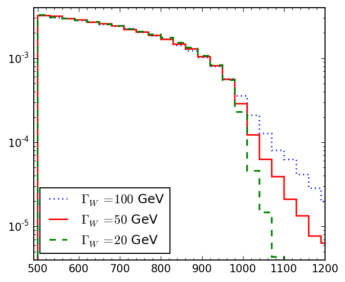
In analogy to Fig. 5, in Fig. 12 we show the distribution for several values of the width, , illustrating the smearing of the kinematic endpoint. The figure suggests that there is sensitivity to the width, but the measurement is challenging, since the effect is concentrated in the region near the endpoint, GeV. We point out that the above measurements can also be performed using the variable [7] — it similarly has a well defined kinematic endpoint, which will be partially smeared by the width effects.

As in the case of single production, for the measurement of the mass scale one cannot rely on endpoint measurements alone and needs to utilize the shapes of the relevant kinematic distributions. Fig. 13 depicts several variables whose distributions show sensitivity to the overall mass scale.


As in Fig. 3, we only consider mass spectra which obey the relation (8) and therefore satisfy the measured (or ) kinematic endpoint. More specifically, we vary the mass, , of the invisible particle as shown in each panel, then choose the parent mass, , from eq. (9). The main effect of the mass scale is to provide a different boost of the parent particles: lighter (heavier) s will be produced with a higher (lower) boost. While the parent boost itself is unobservable, its effects are reflected in the kinematic distributions of the visible decay products. For example, when the s are highly boosted in the transverse plane, we would expect the leptons to be back to back. Any time the s are highly boosted in the CM frame (whether in the transverse plane or along the beam axis) we expect a larger invariant mass of the visible leptons, as well as higher (on average) values of their transverse and longitudinal momenta. These expectations are confirmed by Fig. 13, in which we show distributions of the dilepton invariant mass, (upper left panel), the transverse lepton momentum, (upper right panel), and the longitudinal lepton momenta (lower two panels). We note that the boost effect is seen better in the distribution of the larger of the two longitudinal lepton momenta (in absolute value), , which is shown in the lower left panel. The other longitudinal lepton momentum, , is then plotted in the lower right panel, with the sign chosen so that it is positive (negative) when the two longitudinal lepton momenta have equal (opposite) signs.
Fig. 13 demonstrates that the kinematic distributions of the visible particles do, in principle, contain information about the mass scale, which can then be extracted from a fit to these (one-dimensional) distributions, as was done in Fig. 4. However, the MEM will have better sensitivity, as it takes into account the correlations among the different variables.
Parameter measurements in the case of pair production with the MEM. In analogy to single production, we now apply the MEM to measure simultaneously the mass scale, the width (Fig. 14), and the chirality of the lepton couplings (Fig. 15). As expected, the MEM is quite successful in determining all the parameters in (1).

In particular, the symbol in Fig. 14 denotes the result from our fit, which is close to the input parameter values (marked with ).


In Fig. 15, a minimum of the negative log-likelihood distribution is always found at the true input value for the chirality (marked with a vertical dotted line). Note that in general, the chirality is determined only up to a two-fold ambiguity, , reflecting the symmetry of the underlying squared amplitude.
The results displayed in Figs. 14 and 15 demonstrate the power of the MEM for parameter measurements in the challenging event topology of Fig. 1(b), thus generalizing and strengthening the conclusions from the previous studies performed in Refs. [38, 39, 40].
Conclusions. We have presented methods to measure masses, widths, and couplings, and, in particular, shown that (a) all of these parameters can be simultaneously measured using the MEM and (b) that the physics which gives sensitivity to each of these parameters is more transparent than it would be with many MVAs. While we have focused on the case of s/ s, the approach and conclusions can be readily generalized to nearly any SM or BSM scenario. We therefore look forward to the utilization of such methods during the continued successful operation of the LHC.
Acknowledgements. K.M. would like to thank his CMS colleagues for useful discussions. AB and DD thank O. Mattelaer for technical help and advice. Work supported in part by U.S. Department of Energy Grants DE-SC0010296 and DE-SC0010504. AB is grateful for the hospitality of the high energy theory group at the University of Florida and acknowledges support from Fulbright and Colciencias. DD acknowledges support from the University of Florida Informatics Institute in the form of a Graduate Student Fellowship. This work was performed in part at the Aspen Center for Physics, which is supported by National Science Foundation grant PHY-1607611.
References
- [1] For a review, see, e.g., J. L. Feng, “Dark Matter Candidates from Particle Physics and Methods of Detection,” Ann. Rev. Astron. Astrophys. 48, 495 (2010) doi:10.1146/annurev-astro-082708-101659 [arXiv:1003.0904 [astro-ph.CO]].
- [2] I. Hinchliffe, F. E. Paige, M. D. Shapiro, J. Soderqvist and W. Yao, “Precision SUSY measurements at CERN LHC,” Phys. Rev. D 55, 5520 (1997) doi:10.1103/PhysRevD.55.5520 [hep-ph/9610544].
- [3] J. Smith, W. L. van Neerven and J. A. M. Vermaseren, “The Transverse Mass and Width of the Boson,” Phys. Rev. Lett. 50, 1738 (1983). doi:10.1103/PhysRevLett.50.1738
- [4] V. D. Barger, A. D. Martin and R. J. N. Phillips, “Perpendicular Mass From Decay,” Z. Phys. C 21, 99 (1983). doi:10.1007/BF01648783
- [5] C. G. Lester and D. J. Summers, “Measuring masses of semiinvisibly decaying particles pair produced at hadron colliders,” Phys. Lett. B 463, 99 (1999) doi:10.1016/S0370-2693(99)00945-4 [hep-ph/9906349].
- [6] A. Barr, C. Lester and P. Stephens, “m(T2): The Truth behind the glamour,” J. Phys. G 29, 2343 (2003) doi:10.1088/0954-3899/29/10/304 [hep-ph/0304226].
- [7] D. R. Tovey, “On measuring the masses of pair-produced semi-invisibly decaying particles at hadron colliders,” JHEP 0804, 034 (2008) doi:10.1088/1126-6708/2008/04/034 [arXiv:0802.2879 [hep-ph]].
- [8] P. Konar, K. Kong, K. T. Matchev and M. Park, “Superpartner Mass Measurement Technique using 1D Orthogonal Decompositions of the Cambridge Transverse Mass Variable ,” Phys. Rev. Lett. 105, 051802 (2010) doi:10.1103/PhysRevLett.105.051802 [arXiv:0910.3679 [hep-ph]].
- [9] K. T. Matchev and M. Park, “A General method for determining the masses of semi-invisibly decaying particles at hadron colliders,” Phys. Rev. Lett. 107, 061801 (2011) doi:10.1103/PhysRevLett.107.061801 [arXiv:0910.1584 [hep-ph]].
- [10] W. T. Giele and S. Keller, “Determination of boson properties at hadron colliders,” Phys. Rev. D 57, 4433 (1998) doi:10.1103/PhysRevD.57.4433 [hep-ph/9704419].
- [11] B. Gripaios, “Transverse observables and mass determination at hadron colliders,” JHEP 0802, 053 (2008) doi:10.1088/1126-6708/2008/02/053 [arXiv:0709.2740 [hep-ph]].
- [12] A. J. Barr, B. Gripaios and C. G. Lester, “Weighing Wimps with Kinks at Colliders: Invisible Particle Mass Measurements from Endpoints,” JHEP 0802, 014 (2008) doi:10.1088/1126-6708/2008/02/014 [arXiv:0711.4008 [hep-ph]].
- [13] W. S. Cho, K. Choi, Y. G. Kim and C. B. Park, “Gluino Stransverse Mass,” Phys. Rev. Lett. 100, 171801 (2008) doi:10.1103/PhysRevLett.100.171801 [arXiv:0709.0288 [hep-ph]].
- [14] W. S. Cho, K. Choi, Y. G. Kim and C. B. Park, “Measuring superparticle masses at hadron collider using the transverse mass kink,” JHEP 0802, 035 (2008) doi:10.1088/1126-6708/2008/02/035 [arXiv:0711.4526 [hep-ph]].
- [15] M. Burns, K. Kong, K. T. Matchev and M. Park, “Using Subsystem MT2 for Complete Mass Determinations in Decay Chains with Missing Energy at Hadron Colliders,” JHEP 0903, 143 (2009) doi:10.1088/1126-6708/2009/03/143 [arXiv:0810.5576 [hep-ph]].
- [16] A. J. Barr, B. Gripaios and C. G. Lester, “Transverse masses and kinematic constraints: from the boundary to the crease,” JHEP 0911, 096 (2009) doi:10.1088/1126-6708/2009/11/096 [arXiv:0908.3779 [hep-ph]].
- [17] K. T. Matchev, F. Moortgat, L. Pape and M. Park, “Precision sparticle spectroscopy in the inclusive same-sign dilepton channel at LHC,” Phys. Rev. D 82, 077701 (2010) doi:10.1103/PhysRevD.82.077701 [arXiv:0909.4300 [hep-ph]].
- [18] P. Konar, K. Kong, K. T. Matchev and M. Park, “Dark Matter Particle Spectroscopy at the LHC: Generalizing M(T2) to Asymmetric Event Topologies,” JHEP 1004, 086 (2010) doi:10.1007/JHEP04(2010)086 [arXiv:0911.4126 [hep-ph]].
- [19] K. Kondo, “Dynamical Likelihood Method for Reconstruction of Events With Missing Momentum. 1: Method and Toy Models,” J. Phys. Soc. Jap. 57, 4126 (1988).
- [20] K. Kondo, “Dynamical likelihood method for reconstruction of events with missing momentum. 2: Mass spectra for processes,” J. Phys. Soc. Jap. 60, 836 (1991).
- [21] K. Kondo, T. Chikamatsu and S. H. Kim, “Dynamical likelihood method for reconstruction of events with missing momentum. 3: Analysis of a CDF high p(T) e mu event as t anti-t production,” J. Phys. Soc. Jap. 62, 1177 (1993).
- [22] R. H. Dalitz and G. R. Goldstein, “The Decay and polarization properties of the top quark,” Phys. Rev. D 45, 1531 (1992).
- [23] B. Abbott et al. [D0 Collaboration], “Measurement of the top quark mass in the dilepton channel,” Phys. Rev. D 60, 052001 (1999) [hep-ex/9808029].
- [24] J. C. Estrada Vigil, “Maximal use of kinematic information for the extraction of the mass of the top quark in single-lepton t anti-t events at D0,” FERMILAB-THESIS-2001-07.
- [25] M. F. Canelli, “Helicity of the boson in single - lepton events,” UMI-31-14921.
- [26] V. M. Abazov et al. [D0 Collaboration], “A precision measurement of the mass of the top quark,” Nature 429, 638 (2004) [hep-ex/0406031].
- [27] J. S. Gainer, J. Lykken, K. T. Matchev, S. Mrenna and M. Park, “The Matrix Element Method: Past, Present, and Future,” arXiv:1307.3546 [hep-ph].
- [28] P. C. Bhat, “Multivariate Analysis Methods in Particle Physics,” Ann. Rev. Nucl. Part. Sci. 61, 281 (2011).
- [29] S. Chatrchyan et al. [CMS Collaboration], “Observation of a new boson at a mass of 125 GeV with the CMS experiment at the LHC,” Phys. Lett. B 716, 30 (2012) [arXiv:1207.7235 [hep-ex]].
- [30] S. Chatrchyan et al. [CMS Collaboration], “Study of the Mass and Spin-Parity of the Higgs Boson Candidate Via Its Decays to Z Boson Pairs,” Phys. Rev. Lett. 110, no. 8, 081803 (2013) doi:10.1103/PhysRevLett.110.081803 [arXiv:1212.6639 [hep-ex]].
- [31] G. Aad et al. [ATLAS Collaboration], “Evidence for the spin-0 nature of the Higgs boson using ATLAS data,” Phys. Lett. B 726, 120 (2013) doi:10.1016/j.physletb.2013.08.026 [arXiv:1307.1432 [hep-ex]].
- [32] S. Chatrchyan et al. [CMS Collaboration], “Measurement of the properties of a Higgs boson in the four-lepton final state,” Phys. Rev. D 89, no. 9, 092007 (2014) doi:10.1103/PhysRevD.89.092007 [arXiv:1312.5353 [hep-ex]].
- [33] Y. Gao, A. V. Gritsan, Z. Guo, K. Melnikov, M. Schulze and N. V. Tran, “Spin determination of single-produced resonances at hadron colliders,” Phys. Rev. D 81, 075022 (2010) [arXiv:1001.3396 [hep-ph]];
- [34] A. De Rujula, J. Lykken, M. Pierini, C. Rogan and M. Spiropulu, “Higgs look-alikes at the LHC,” Phys. Rev. D 82, 013003 (2010) [arXiv:1001.5300 [hep-ph]];
- [35] S. Bolognesi, Y. Gao, A. V. Gritsan, K. Melnikov, M. Schulze, N. V. Tran and A. Whitbeck, “On the spin and parity of a single-produced resonance at the LHC,” Phys. Rev. D 86, 095031 (2012) [arXiv:1208.4018 [hep-ph]].
- [36] P. Avery, D. Bourilkov, M. Chen, T. Cheng, A. Drozdetskiy, J. S. Gainer, A. Korytov and K. T. Matchev et al., “Precision studies of the Higgs boson decay channel HZZ with MEKD,” Phys. Rev. D 87, no. 5, 055006 (2013) [arXiv:1210.0896 [hep-ph]].
- [37] M. Chen, T. Cheng, J. S. Gainer, A. Korytov, K. T. Matchev, P. Milenovic, G. Mitselmakher and M. Park et al., “The role of interference in unraveling the ZZ-couplings of the newly discovered boson at the LHC,” Phys. Rev. D 89, 034002 (2014) [arXiv:1310.1397 [hep-ph]].
- [38] J. Alwall, A. Freitas and O. Mattelaer, “Measuring Sparticles with the Matrix Element,” AIP Conf. Proc. 1200, 442 (2010) doi:10.1063/1.3327611 [arXiv:0910.2522 [hep-ph]].
- [39] P. Artoisenet, V. Lemaitre, F. Maltoni and O. Mattelaer, “Automation of the matrix element reweighting method,” JHEP 1012, 068 (2010) doi:10.1007/JHEP12(2010)068 [arXiv:1007.3300 [hep-ph]].
- [40] C. Y. Chen and A. Freitas, “General analysis of signals with two leptons and missing energy at the Large Hadron Collider,” JHEP 1102, 002 (2011) doi:10.1007/JHEP02(2011)002 [arXiv:1011.5276 [hep-ph]].
- [41] W. Altmannshofer, J. Eby, S. Gori, M. Lotito, M. Martone and D. Tuckler, “Collider Signatures of Flavorful Higgs Bosons,” Phys. Rev. D 94, no. 11, 115032 (2016) doi:10.1103/PhysRevD.94.115032 [arXiv:1610.02398 [hep-ph]].
- [42] J. Kalinowski, R. Ruckl, H. Spiesberger and P. M. Zerwas, “R-parity violating SUSY signals in lepton pair production at the Tevatron,” Phys. Lett. B 414, 297 (1997) doi:10.1016/S0370-2693(97)01184-2 [hep-ph/9708272].
- [43] J. L. Hewett and T. G. Rizzo, “Resonant slepton production at hadron colliders in R-parity violating models,” In *Vancouver 1998, High energy physics, vol. 2* 1698-1702 [hep-ph/9809525].
- [44] V. Khachatryan et al. [CMS Collaboration], “Search for heavy gauge W’ boson in events with an energetic lepton and large missing transverse momentum at 13 TeV,” Phys. Lett. B 770, 278 (2017) doi:10.1016/j.physletb.2017.04.043 [arXiv:1612.09274 [hep-ex]].
- [45] M. Aaboud et al. [ATLAS Collaboration], “Search for a new heavy gauge boson resonance decaying into a lepton and missing transverse momentum in 36 fb-1 of collisions at 13 TeV with the ATLAS experiment,” arXiv:1706.04786 [hep-ex].
- [46] E. Eichten, I. Hinchliffe, K. D. Lane and C. Quigg, “Super Collider Physics,” Rev. Mod. Phys. 56, 579 (1984) Addendum: [Rev. Mod. Phys. 58, 1065 (1986)]. doi:10.1103/RevModPhys.56.579, 10.1103/RevModPhys.58.1065
- [47] S. S. D. Willenbrock, “Pair Production of Supersymmetric Charged Higgs Bosons,” Phys. Rev. D 35, 173 (1987). doi:10.1103/PhysRevD.35.173
- [48] A. Belyaev, C. R. Chen, K. Tobe and C.-P. Yuan, “Phenomenology of littlest Higgs model with parity: including effects of odd fermions,” Phys. Rev. D 74, 115020 (2006) doi:10.1103/PhysRevD.74.115020 [hep-ph/0609179].
- [49] R. Barbieri, F. Caravaglios, M. Frigeni and M. L. Mangano, “Production and leptonic decays of charginos and neutralinos in hadronic collisions,” Nucl. Phys. B 367, 28 (1991). doi:10.1016/0550-3213(91)90040-5
- [50] H. C. Cheng, K. T. Matchev and M. Schmaltz, “Bosonic supersymmetry? Getting fooled at the CERN LHC,” Phys. Rev. D 66, 056006 (2002) doi:10.1103/PhysRevD.66.056006 [hep-ph/0205314].
- [51] A. J. Barr, “Measuring slepton spin at the LHC,” JHEP 0602, 042 (2006) doi:10.1088/1126-6708/2006/02/042 [hep-ph/0511115].
- [52] F. del Aguila and L. Ametller, “On the detectability of sleptons at large hadron colliders,” Phys. Lett. B 261, 326 (1991). doi:10.1016/0370-2693(91)90336-O
- [53] H. Baer, C. h. Chen, F. Paige and X. Tata, “Detecting Sleptons at Hadron Colliders and Supercolliders,” Phys. Rev. D 49, 3283 (1994) doi:10.1103/PhysRevD.49.3283 [hep-ph/9311248].
- [54] J. S. Gainer, J. Lykken, K. T. Matchev, S. Mrenna and M. Park, “Exploring Theory Space with Monte Carlo Reweighting,” JHEP 1410, 78 (2014) [arXiv:1404.7129 [hep-ph]].
- [55] J. Alwall, M. Herquet, F. Maltoni, O. Mattelaer and T. Stelzer, “MadGraph 5 : Going Beyond,” JHEP 1106, 128 (2011) [arXiv:1106.0522 [hep-ph]].
- [56] P. Artoisenet and O. Mattelaer, “MadWeight: Automatic event reweighting with matrix elements,” PoS CHARGED 2008, 025 (2008).
- [57] A. Buckley, J. Ferrando, S. Lloyd, K. Nordström, B. Page, M. Rüfenacht, M. Schönherr and G. Watt, “LHAPDF6: parton density access in the LHC precision era,” Eur. Phys. J. C 75, 132 (2015) doi:10.1140/epjc/s10052-015-3318-8 [arXiv:1412.7420 [hep-ph]].
- [58] Y. Grossman, M. Martone and D. J. Robinson, “Kinematic Edges with Flavor Oscillation and Non-Zero Widths,” JHEP 1110, 127 (2011) doi:10.1007/JHEP10(2011)127 [arXiv:1108.5381 [hep-ph]].
- [59] D. J. Summers, “Transverse mass as a means of measuring the width at the Tevatron,” Phys. Lett. B 392, 216 (1997) doi:10.1016/S0370-2693(96)01493-1 [hep-ph/9608332].
- [60] T. G. Rizzo, “The Determination of the Helicity of Boson Couplings at the LHC,” JHEP 0705, 037 (2007) doi:10.1088/1126-6708/2007/05/037 [arXiv:0704.0235 [hep-ph]].
- [61] M. Burns, K. Kong, K. T. Matchev and M. Park, “A General Method for Model-Independent Measurements of Particle Spins, Couplings and Mixing Angles in Cascade Decays with Missing Energy at Hadron Colliders,” JHEP 0810, 081 (2008) doi:10.1088/1126-6708/2008/10/081 [arXiv:0808.2472 [hep-ph]].