跳到论文正文
W Papers独立论文阅读器 arXiv:1708.06960 论文正文 计算阅读时间 · 0%
引用这篇论文根据当前论文元数据生成,正式投稿前建议核对。


License: arXiv.org perpetual non-exclusive license
arXiv:1708.06960v2 [math.MG] 09 Feb 2018

A four point characterisation for coarse median spacesThanks: Partially supported by the Sino-British Fellowship Trust by Royal Society.

Graham A. Niblo , Nick Wright and Jiawen Zhang Address: School of Mathematics, University of Southampton, Highfield, SO17 1BJ, United Kingdom. Email address: {g.a.niblo,n.j.wright,jiawen.zhang}@soton.ac.uk
Abstract.

Coarse median spaces simultaneously generalise the classes of hyperbolic spaces and median algebras, and arise naturally in the study of the mapping class groups and many other contexts. Their definition as originally conceived by Bowditch requires median approximations for all finite subsets of the space. Here we provide a simplification of the definition in the form of a 44-point condition analogous to Gromov’s 44-point condition defining hyperbolicity. We give an intrinsic characterisation of rank in terms of the coarse median operator and use this to give a direct proof that rank 11 geodesic coarse median spaces are δ\delta-hyperbolic, bypassing Bowditch’s use of asymptotic cones. A key ingredient of the proof is a new definition of intervals in coarse median spaces and an analysis of their interaction with geodesics.

Key words and phrases: 
Coarse median space, canonical metric, hyperbolicity, rank
2010 Mathematics Subject Classification
20F65, 20F67, 20F69

1. Introduction

Coarse median spaces and groups were introduced by Bowditch in 2013 [5] as a coarse variant of classical median algebras. The notion of a coarse median group leads to a unified viewpoint on several interesting classes, including Gromov’s hyperbolic groups, mapping class groups, and CAT(0) cubical groups. Bowditch showed that geodesic hyperbolic spaces are exactly geodesic coarse median spaces of rank 1, and mapping class groups are examples of coarse median spaces of finite rank [5]. In 2014 [3, 4], Behrstoke, Hagen and Sisto introduced the notion of hierarchically hyperbolic spaces, and showed that these are coarse median.

Intuitively, a coarse median space (X,d,μ)(X,d,\mu) is a metric space (X,d)(X,d) equipped with a ternary operator μ\mu (called the coarse median), in which every finite subset can be approximated by a finite CAT(0) cube complex, with distortion controlled by the metric. This can be viewed as a wide-ranging extension of Gromov’s observation that in a δ\delta-hyperbolic space finite subsets can be approximated by trees. See also Zeidler’s Master’s thesis [23].

In this paper we simplify the definition of a coarse median space, replacing the requirement to approximate arbitrary finite subsets with a simplified 44-point condition which may be viewed as a high dimensional analogue of Gromov’s 44-point condition for hyperbolicity. Our condition asserts that given any four points a,b,c,da,b,c,d the two iterated coarse medians μ⁡(μ⁡(a,b,c),b,d)\mu(\mu(a,b,c),b,d) and μ⁡(a,b,μ⁡(c,b,d))\mu(a,b,\mu(c,b,d)) are uniformly close. As illustrated below this corresponds to an approximation by a CAT(0) cube complex of dimension 33, where the corresponding iterated medians coincide.

Figure 1. The CAT(0) cube complex associated to the free median algebra on {a,b,c,d}\{a,b,c,d\}

We recall that Gromov gave a 44-point condition characterising hyperbolicity for geodesic spaces which, in essence, asserts that any four points can be approximated by one of the trees shown in Figure 2.

Figure 2. Gromov’s 44-point condition

We can visualise each of these trees as degenerate cases of Figure 1 in which two of the dimensions of the cube are collapsed, making clear the relationship between Gromov’s 44-point condition and ours, and the sense in which coarse median spaces are a higher dimensional analogue of δ\delta-hyperbolic spaces. The presence of the central 33-cube, which may be arbitrarily large, allows for flat geometry.

The coarse 44-point condition is also a coarse analogue of the 44-point characterisation for median algebras, as introduced and studied by Kolibiar and Marcisová in [13]. To establish the equivalence with Bowditch’s original definition we introduce a model for the free median algebra generated by nn points, which may be of independent interest.

Any median algebra generated by 44 points can be modelled by the 33-dimensional CAT(0) cube complex illustrated in Figure 1, so it is a priori difficult to see how to characterise rank using our new definition. We overcome this by offering several intrinsic characterisations of rank in terms of the coarse median operator itself and which are equivalent to Bowditch’s definition.

The rank 1 geodesic case is of independent interest, since, as remarked above, it coincides with the class of geodesic hyperbolic spaces, [5]. Bowditch’s proof that rank 11 geodesic coarse median spaces are hyperbolic uses an ingenious asymptotic cones argument which conceals in part the strong interaction between quasi-geodesics and coarse median intervals in this case. Introducing a new definition of interval in a coarse median space, we give an alternative proof, bypassing the asymptotic cones argument, and instead exploiting a result of Papasoglu [17] and Pomroy [18], see also [9]. We also consider the behaviour of quasi-geodesics in higher rank coarse median spaces, giving an example in rank 22 to show that even geodesics can wander far from the intervals defined by the coarse median operator. In a subsequent paper, [15] we further develop the concept of the coarse interval structure associated to a coarse median space and, as an application, we show there that the metric data is determined by the coarse median operator itself.

The paper is organised as follows. In Section 2, we recall Bowditch’s definition of coarse median spaces and introduce our notion of (coarse) intervals (which differ in one small but crucial respect from the intervals studied by Bowditch). In Section 3, we establish our 44-point condition characterising coarse median spaces. In Section 4, we give several characterisations for rank in terms of the coarse median operator and give a new proof of Bowditch’s result concerning the hyperbolicity of rank 11 geodesic coarse median spaces. Finally in Section 5, we construct an example to show that geodesics do not have to remain close to intervals in a coarse median space of rank greater than 11.

2. Preliminaries

2.1. Metrics and geodesics

Definition 2.1.

Let (X,d)(X,d) and (Y,d′)(Y,d^{\prime}) be metric spaces.

  1. (1)

    (X,d)(X,d) is said to be quasi-geodesic, if there exist constants L,C>0L,C>0 such that for any two points x,y∈Xx,y\in X, there exists a map γ:[0,d⁡(x,y)]→X\gamma\colon[0,d(x,y)]\rightarrow X with γ⁡(0)=x\gamma(0)=x, γ⁡(d⁡(x,y))=y\gamma(d(x,y))=y, satisfying: for any s,t∈[0,d⁡(x,y)]s,t\in[0,d(x,y)],

    L−1​|s−t|−C⩽d⁡(γ⁡(s),γ⁡(t))⩽L|s−t|+C.L^{-1}|s-t|-C\leqslant d(\gamma(s),\gamma(t))\leqslant L|s-t|+C.

    If we care about the constants we say that (X,d)(X,d) is (L,C)(L,C)-quasi-geodesic, and if we do not care about the constant CC we say that (X,d)(X,d) is LL-quasi-geodesic. If (X,d)(X,d) is (1,0)(1,0)-quasi-geodesic then we say that XX is geodesic. When considering integer-valued metrics we make the same definitions restricting the intervals to intervals in ℤ\mathbb{Z}.

  2. (2)

    A map f:(X,d)→(Y,d′)f:(X,d)\rightarrow(Y,d^{\prime}) is bornologous if there exists an increasing map ρ+:ℝ+→ℝ+\rho_{+}:\mathbb{R}^{+}\rightarrow\mathbb{R}^{+} such that for all x,y∈Xx,y\in X, d′​(f⁡(x),f⁡(y))⩽ρ+​(d⁡(x,y))d^{\prime}(f(x),f(y))\leqslant\rho_{+}(d(x,y)).

  3. (3)

    (X,d)(X,d) is said to be uniformly discrete if there exists a constant C>0C>0 such that for any x≠y∈Xx\neq y\in X, d⁡(x,y)⩾Cd(x,y)\geqslant C.

  4. (4)

    Two points x,y∈Xx,y\in X are said to be ss-close (with respect to the metric dd) if d⁡(x,y)⩽sd(x,y)\leqslant s. If xx is ss-close to yy we write x∼syx\thicksim_{s}y.

2.2. CAT(0) Cube Complexes

Before considering coarse median spaces, we first recall basic notions and results about CAT(0) cube complexes. We will survey the properties we need here, but guide the interested reader to [7, 10, 11, 14, 20] for more information.

A cube complex is a polyhedral complex in which each cell is isometric to a unit Euclidean cube and the gluing maps are isometries. The dimension of the complex is the maximum of the dimensions of the cubes. For a cube complex XX, we can associate it with the intrinsic pseudo-metric di​n​td_{int}, which is the maximal pseudo-metric on XX such that each cube embeds isometrically. When XX is connected and has finite dimension, di​n​td_{int} is a complete geodesic metric on XX. See [7] for a general discussion on polyhedral complex and the associated intrinsic metric. A geodesic metric space is CAT(0) if all its geodesic triangles are slimmer than the comparative triangle in the Euclidean space. For a cube complex (X,di​n​t)(X,d_{int}), Gromov gave a combinatorial characterisation of the CAT(0) condition [11]: XX is CAT(0) if and only if it is simply connected and the link of each vertex is a flag complex (see also [7]).

We also consider the edge path metric dd on the vertex set VV of a CAT(0) cube complex. For x,y∈Vx,y\in V, the interval is defined to be [x,y]={z∈V:d⁡(x,y)=d⁡(x,z)+d⁡(x,y)}[x,y]=\{z\in V:d(x,y)=d(x,z)+d(x,y)\}, which consists of points on any edge path geodesic between xx and yy. A CAT(0) cubical complex XX can be equipped with a set of hyperplanes [8, 14, 16, 20] such that each edge is crossed by exactly one hyperplane. Each hyperplane divides the space into two halfspaces, and the metric dd counts the number of hyperplanes separating a pair of points. The dimension of XX, if it is finite, is the maximal number of pairwise intersecting hyperplanes. We say that a subset is convex if it is an intersection of half spaces, and we can equivalently define the interval [x,y][x,y] to be the intersection of all the halfspaces containing both xx and yy.

Another characterisation of the CAT(0) condition was obtained by Chepoi [10] (see also [19]): a flag cube complex XX is CAT(0) if and only if for any x,y,z∈Vx,y,z\in V, the intersection [x,y]∩[y,z]∩[z,x][x,y]\cap[y,z]\cap[z,x] consists of a single point μ⁡(x,y,z)\mu(x,y,z), which is called the median of x,y,zx,y,z. Obviously, m⁡(x,y,z)∈[x,y]m(x,y,z)\in[x,y], and

[x,y]={m⁡(x,y,z):z∈V}={w∈V:m⁡(x,y,w)=w}[x,y]=\{m(x,y,z):z\in V\}=\{w\in V:m(x,y,w)=w\}

A graph such as X(1)X^{(1)} satisfying this condition is called a median graph.

Given a CAT(0) cube complex, we always take the canonical median structure (V,m)(V,m) defined by intersection of intervals as above. The pair (V,m)(V,m) is a median algebra [12], as defined in the following section.

2.3. Median Algebras

As discussed in [1], there are a number of equivalent formulations of the axioms for median algebras. We will use the following formulation from [13], see also [2]:

Definition 2.2.

Let XX be a set and mm a ternary operation on XX. Then mm is a median operator and the pair (X,m)(X,m) is a median algebra if:

  • (M1) Localisation:

    m⁡(a,a,b)=am(a,a,b)=a;

  • (M2) Symmetry:

    m⁡(a1,a2,a3)=m⁡(aσ⁡(1),aσ⁡(2),aσ⁡(3))m(a_{1},a_{2},a_{3})=m(a_{\sigma(1)},a_{\sigma(2)},a_{\sigma(3)}), where σ\sigma is any permutation of {1,2,3}\{1,2,3\};

  • (M3) The 4-point condition:

    m⁡(m⁡(a,b,c),b,d)=m⁡(a,b,m⁡(c,b,d))m(m(a,b,c),b,d)=m(a,b,m(c,b,d)).

Condition (M3) is illustrated by Figure 1, which shows the free median algebra generated by the 44 points a,b,c,da,b,c,d. As shown in the figure, the iterated medians on both sides of the equality in (M3) evaluate to the vertex adjacent to bb.

Example 2.3.

An important example is furnished by the “median nn-cube”, denoted by InI^{n}, which is the nn-dimensional vector space over ℤ2\mathbb{Z}_{2} with the median operator μn\mu_{n} given by majority vote on each coordinate.

Definition 2.4.

The rank of a median algebra (X,m)(X,m) is the supremum of those nn for which there is a subalgebra of (X,m)(X,m) isomorphic to the median algebra (In,μn)(I^{n},\mu_{n}).

For the median algebra defined by the vertex set of a CAT(0) cube complex, the rank coincides with the dimension of the cube complex.

For any points a,b∈Xa,b\in X we define the interval between a,ba,b to be

[a,b]:={m⁡(a,x,b):x∈X}.[a,b]:=\{m(a,x,b):x\in X\}.

Axioms (M1) ∼\sim (M3) ensure that [a,b][a,b] is also equal to the set {c∈X:m⁡(a,c,b)=c}\{c\in X:m(a,c,b)=c\}, since if c=m⁡(a,b,x)c=m(a,b,x) then:

m⁡(c,a,b)=m⁡(m⁡(x,a,b),a,b)=m⁡(x,m⁡(a,b,a),b)=m⁡(x,a,b)=c.m(c,a,b)=m(m(x,a,b),a,b)=m(x,m(a,b,a),b)=m(x,a,b)=c.

We think of m⁡(a,x,b)m(a,x,b) as the projection of xx onto the interval [a,b][a,b], and axiom (M3) can be viewed as an associativity axiom: For each b∈Xb\in X the binary operator

(a,c)↦a∗bc:=m⁡(a,b,c)(a,c)\mapsto a*_{b}c:=m(a,b,c)

is associative. It is also commutative by (M2) and iterated projection gives rise to the iterated median introduced in [21].

Definition 2.5 ([21]).

Let (X,m)(X,m) be a median algebra. For x1∈Xx_{1}\in X, define

m⁡(x1,b):=x1,m(x_{1};b):=x_{1},

and for k⩾1k\geqslant 1 and x1,…,xk+1∈Xx_{1},\ldots,x_{k+1}\in X, define

m⁡(x1,…,xk+1,b):=m⁡(m⁡(x1,…,xk,b),xk+1,b).m(x_{1},\ldots,x_{k+1};b):=m(m(x_{1},\ldots,x_{k};b),x_{k+1},b).

Note that this definition “agrees” with the original median operator mm, since m⁡(x1,x2,b)=m⁡(x1,x2,b)m(x_{1},x_{2};b)=m(x_{1},x_{2},b).

In the notation above, the definition reduces to:

m(x1,…,xk;b)=x1∗bx2∗b…∗bxk.m(x_{1},\ldots,x_{k};b)=x_{1}*_{b}x_{2}*_{b}\ldots*_{b}x_{k}.

A subset YY of AA is said to be convex if m⁡(x,b,y)∈Ym(x,b,y)\in Y for all x,y∈Yx,y\in Y and b∈Xb\in X, or equivalently, if it is closed under the binary operation ∗b*_{b} for all b∈Xb\in X. The set {m⁡(x1,…,xn,b)∣b∈X}\{~m(x_{1},\ldots,x_{n};b)\mid b\in X~\} is the convex hull of the points xix_{i} and we think of the iterated median m⁡(x1,…,xn,b)m(x_{1},\ldots,x_{n};b) as the projection of bb onto the convex hull.

We recall several properties of the iterated median operator proved in the original paper [21].

Lemma 2.6 ([21]).

Let (X,m)(X,m) be a median algebra, and x1,…,xn,a,b∈Xx_{1},\ldots,x_{n},a,b\in X. Then:

  1. (1)

    The iterated median operator defined above is symmetric in x1,…,xnx_{1},\ldots,x_{n};

  2. (2)

    ⋂k=1n[xk,b]=[m⁡(x1,…,xn,b),b]\bigcap\limits_{k=1}^{n}[x_{k},b]=[m(x_{1},\ldots,x_{n};b),b];

  3. (3)

    If, in addition, XX has rank at most dd, then there exists a subset {y1,…,yk}⊆{x1,…,xn}\{y_{1},\ldots,y_{k}\}\subseteq\{x_{1},\ldots,x_{n}\} with k⩽dk\leqslant d, such that

    m⁡(y1,…,yk,b)=m⁡(x1,…,xn,b);m(y_{1},\ldots,y_{k};b)=m(x_{1},\ldots,x_{n};b);
  4. (4)

    Assume that x1,…,xn∈[a,b]x_{1},\ldots,x_{n}\in[a,b], then {x1,…,xn}⊆[a,m⁡(x1,…,xn,b)]\{x_{1},\ldots,x_{n}\}\subseteq[a,m(x_{1},\ldots,x_{n};b)].

We remark that condition (1) here follows immediately from the commutativity and associativity of the binary operator ∗b*_{b}.

We will also make use of the following “(n+2)-point condition”.

Lemma 2.7.

Let (X,m)(X,m) be a median algebra and a,b,e1,…,en+1∈Xa,b,e_{1},\ldots,e_{n+1}\in X, then

m⁡(a,en+1,m⁡(e1,…,en,b))=m⁡(m⁡(a,en+1,e1),…,m⁡(a,en+1,en),b).m(a,e_{n+1},m(e_{1},\ldots,e_{n};b))=m(m(a,e_{n+1},e_{1}),\ldots,m(a,e_{n+1},e_{n});b).
Proof.

We prove this by induction on nn.

n=1n=1: the equation holds trivially. Assume it holds for all k⩽nk\leqslant n. Then

m⁡(a,en+1,m⁡(e1,…,en,b))=m⁡(a,en+1,m⁡(m⁡(e1,…,en−1,b),en,b))\displaystyle m(a,e_{n+1},m(e_{1},\ldots,e_{n};b))=m\big(a,e_{n+1},m(m(e_{1},\ldots,e_{n-1};b),e_{n},b)\big)
=\displaystyle= m⁡(m⁡(a,en+1,m⁡(e1,…,en−1,b)),m⁡(a,en+1,en),b)\displaystyle m\big(m(a,e_{n+1},m(e_{1},\ldots,e_{n-1};b)),m(a,e_{n+1},e_{n}),b\big)
=\displaystyle= m⁡(m⁡(m⁡(a,en+1,e1),…,m⁡(a,en+1,en−1),b),m⁡(a,en+1,en),b)\displaystyle m\big(m(m(a,e_{n+1},e_{1}),\ldots,m(a,e_{n+1},e_{n-1});b),m(a,e_{n+1},e_{n}),b\big)
=\displaystyle= m⁡(m⁡(a,en+1,e1),…,m⁡(a,en+1,en),b),\displaystyle m(m(a,e_{n+1},e_{1}),\ldots,m(a,e_{n+1},e_{n});b),

where we use the inductive assumption in the third equation. ∎

We now mention two alternative definitions for median algebras.

According to Isbell [12], a ternary operator mm defines a median if and only if it satisfies (M1), (M2) and Isbell’s condition:

m⁡(a,m⁡(a,b,c),m⁡(b,c,d))=m⁡(a,b,c).m(a,m(a,b,c),m(b,c,d))=m(a,b,c).

This says that m⁡(a,b,c)m(a,b,c) is in the interval from aa to m⁡(b,c,d)m(b,c,d), or in geometrical terms that the projection of aa onto [b,c][b,c] provided by the median lies between aa and every other point (m⁡(b,c,d)m(b,c,d)) of the interval [b,c][b,c].

An alternative and algebraically powerful formulation, is that (X,m)(X,m) is a median algebra if it satisfies (M1), (M2) and the five point condition:

m⁡(m⁡(a,b,c),d,e)=m⁡(a,m⁡(b,d,e),m⁡(c,d,e)),m(m(a,b,c),d,e)=m(a,m(b,d,e),m(c,d,e)),

which is the n=3n=3 case of Lemma 2.7. Setting e=be=b one recovers (M3), while

m⁡(a,m⁡(d,b,c),(a,b,c))=m⁡(m⁡(a,d,a),b,c)=m⁡(a,b,c)m(a,m(d,b,c),(a,b,c))=m(m(a,d,a),b,c)=m(a,b,c)

recovering Isbell’s condition.

2.4. Coarse median spaces

In [5], Bowditch introduced coarse median operators as follows:

Definition 2.8 (Bowditch, [5]).

Given a metric space (X,d)(X,d), a coarse median (operator) on XX is a ternary operator μ:X3→X\mu\colon X^{3}\rightarrow X satisfying the following conditions:

  • (C1).

    There is an affine function ρ⁡(t)=K​t+H0\rho(t)=Kt+H_{0} such that for any a,b,c,a′,b′,c′∈Xa,b,c,a^{\prime},b^{\prime},c^{\prime}\in X,

    d⁡(μ⁡(a,b,c),μ⁡(a′,b′,c′))⩽ρ⁡(d⁡(a,a′)+d⁡(b,b′)+d⁡(c,c′)).d(\mu(a,b,c),\mu(a^{\prime},b^{\prime},c^{\prime}))\leqslant\rho(d(a,a^{\prime})+d(b,b^{\prime})+d(c,c^{\prime})).
  • (C2).

    There is a function H:ℕ→[0,+∞)H\colon\mathbb{N}\rightarrow[0,+\infty), such that for any finite subset A⊆XA\subseteq X with 1⩽|A|⩽p1\leqslant|A|\leqslant p, there exists a finite median algebra (Π,μΠ)(\Pi,\mu_{\Pi}) and maps π:A→Π\pi\colon A\rightarrow\Pi, λ:Π→X\lambda\colon\Pi\rightarrow X such that for any x,y,z∈Π,a∈Ax,y,z\in\Pi,a\in A,

    λμΠ(x,y,z)∼H⁡(p)μ(λx,λy,λz),\lambda\mu_{\Pi}(x,y,z)\thicksim_{H(p)}\mu(\lambda x,\lambda y,\lambda z),

    and

    λπa∼H⁡(p)a.\lambda\pi a\thicksim_{H(p)}a.

    We may assume that Π\Pi is generated by π⁡(A)\pi(A).

We say that two coarse median operators μ1,μ2\mu_{1},\mu_{2} on a metric space (X,d)(X,d) are uniformly close if there is a uniform bound on the set of distances

{d(μ1(a,b,c),μ2(a,b,c))∣a,b,c∈X}.\{d(\mu_{1}(a,b,c),\mu_{2}(a,b,c))\mid a,b,c\in X\}.
Remark 2.9.

The control function ρ\rho in (C1) is required by Bowditch to be affine, however it seems more natural in the context of coarse geometry to allow ρ\rho to be an arbitrary function and indeed much of what we show in this paper works with that variation. This may allow wider applications in the future (in [15] we introduce and study such a generalisation in the context of coarse interval structures), though we note that when XX is a quasi-geodesic space the existence of any control function ρ\rho guarantees that ρ\rho may be replaced by an affine control function as in (C1). In this paper we will assume that ρ\rho is affine throughout, but note that many of the statements and arguments can be suitably adapted to the more general context.

We refer to the functions ρ,H\rho,H appearing in conditions (C1), (C2) as parameters of the coarse median, or since ρ\rho has the form ρ⁡(t)=K​t+H0\rho(t)=Kt+H_{0} we will sometimes refer to K,H0,HK,H_{0},H as parameters of the coarse median. The parameters are not unique, and neither are they part of the data of the coarse median; it is merely their existence which is required.

Remark 2.10.

As noted by Bowditch there is a constant κ0>0{\kappa_{0}}>0 such that:

  • •

    μ(a,a,b)∼κ0a\mu(a,a,b)\thicksim_{{\kappa_{0}}}a;

  • •

    μ(a1,a2,a3)∼κ0μ(aσ⁡(1),aσ⁡(2),aσ⁡(3))\mu(a_{1},a_{2},a_{3})\thicksim_{{\kappa_{0}}}\mu(a_{\sigma(1)},a_{\sigma(2)},a_{\sigma(3)}) for any permutation σ∈S3\sigma\in S_{3}.

It follows that any coarse median operator on (X,d)(X,d) may be replaced by another to which it is uniformly close and which satisfies the first two median axioms (M1) and (M2), i.e. we may always assume that κ0=0{\kappa_{0}}=0. We note here that this is true even if we replace the affine control function by an arbitrary ρ\rho as discussed above, taking κ0=2​ρ​(3​H​(3))+2​H​(3){\kappa_{0}}=2\rho(3H(3))+2H(3).

With this in mind we take the following as our definition of a coarse median space.

Definition 2.11.

A coarse median space is a triple (X,d,μ)(X,d,\mu) where dd is a metric on XX and μ\mu is a ternary operator on XX satisfying conditions (M1), (M2), (C1) and (C2).

A map ff between coarse median spaces (X,dX,μX),(Y,dY,μY)(X,d_{X},\mu_{X}),(Y,d_{Y},\mu_{Y}) is said to be an LL-quasi-morphism if for any a,b,c∈Xa,b,c\in X, μY(f(a),f(b),f(c))∼Lf(μX(a,b,c))\mu_{Y}(f(a),f(b),f(c))\thicksim_{L}f(\mu_{X}(a,b,c)).

We note that given a median algebra any metric on this will satisfy axiom (C2), however the metric must be chosen carefully if we wish it to also satisfy axiom (C1). Of course in the case that the median algebra has finite intervals, and hence arises as the vertex set of a CAT(0) cube complex, then both the intrinsic and edge path metrics satisfy this axiom.

2.5. The rank of a coarse median space

Rank is a proxy for dimension in the context of coarse median spaces, directly analogous to the notion of dimension for a CAT(0) cube complex.

Definition 2.12.

Let nn be a natural number. We say XX has rank at most nn if there exist parameters ρ,H\rho,H for which we can always choose the approximating median algebra Π\Pi in condition (C2) to have rank at most nn.

We remark that for a median algebra equipped with a suitable metric making it a coarse median space, the rank as a median algebra gives an upper bound for the rank as a coarse median space, however these need not agree. For example any finite median algebra has rank 00 as a coarse median space.

Zeidler [23] showed that, at the cost of increasing the rank of the approximating median algebra, one can always assume that the map λ​π\lambda\pi from condition (C2) is the inclusion map ιA:A↪X\iota_{A}\colon A\hookrightarrow X. We will now show that this can be achieved without increasing the rank:

Lemma 2.13.

Assume (X,d,μ)(X,d,\mu) is a coarse median space. Then, at the cost of changing the parameter function HH, one can always change the triples Π,λ,π\Pi,\lambda,\pi provided by axiom (C2), so that λ​π=ιA:A↪X\lambda\pi=\iota_{A}\colon A\hookrightarrow X (the inclusion map), without changing the rank of Π\Pi.

Proof.

Given a finite subset A⊆XA\subseteq X with 1⩽|A|⩽p1\leqslant|A|\leqslant p, let the finite median algebra (Π,μΠ)(\Pi,\mu_{\Pi}) and maps π:A→Π\pi\colon A\rightarrow\Pi, λ:Π→X\lambda\colon\Pi\rightarrow X be as in the definition above.

We now construct another finite median algebra (Π′,μΠ′)(\Pi^{\prime},\mu^{\prime}_{\Pi}). As a set, Π′=Π⊔A\Pi^{\prime}=\Pi\sqcup A. Define a map τ:Π′→Π\tau\colon\Pi^{\prime}\rightarrow\Pi by τ​x=x\tau x=x if x∈Πx\in\Pi, and τ​a=π​a\tau a=\pi a if a∈Aa\in A. Now define a median μΠ′\mu^{\prime}_{\Pi} on Π′\Pi^{\prime} by:

  • •

    μΠ′​(a,a,x)=μΠ′​(a,x,a)=μΠ′​(x,a,a)=a\mu^{\prime}_{\Pi}(a,a,x)=\mu^{\prime}_{\Pi}(a,x,a)=\mu^{\prime}_{\Pi}(x,a,a)=a, if a∈Aa\in A and x∈Π′x\in\Pi^{\prime};

  • •

    μΠ′​(x,y,z)=μΠ​(τ​x,τ​y,τ​z)\mu^{\prime}_{\Pi}(x,y,z)=\mu_{\Pi}(\tau x,\tau y,\tau z), otherwise.

It is a direct calculation to check that μΠ′\mu_{\Pi}^{\prime} satisfies the axioms of a median operator. Now define π′:A→Π′\pi^{\prime}\colon A\rightarrow\Pi^{\prime} by π′​a=a\pi^{\prime}a=a; and λ′:Π′=Π⊔A→X\lambda^{\prime}\colon\Pi^{\prime}=\Pi\sqcup A\rightarrow X by λ′=λ⊔ιA\lambda^{\prime}=\lambda\sqcup\iota_{A}. For any x,y,z∈Π′x,y,z\in\Pi^{\prime}: if two of them are equal and sit in AA, say x=y∈Ax=y\in A, then

λ′​μΠ′​(x,y,z)=λ′​x=x=μ⁡(λ′​x,λ′​y,λ′​z);\lambda^{\prime}\mu_{\Pi}^{\prime}(x,y,z)=\lambda^{\prime}x=x=\mu(\lambda^{\prime}x,\lambda^{\prime}y,\lambda^{\prime}z);

otherwise, we have:

λ′​μΠ′​(x,y,z)\displaystyle\lambda^{\prime}\mu_{\Pi}^{\prime}(x,y,z) =\displaystyle= λ′​μΠ​(τ​x,τ​y,τ​z)=λ​μΠ​(τ​x,τ​y,τ​z)\displaystyle\lambda^{\prime}\mu_{\Pi}(\tau x,\tau y,\tau z)\quad=\quad\lambda\mu_{\Pi}(\tau x,\tau y,\tau z)
∼H⁡(p)\displaystyle\thicksim_{H(p)} μ(λ′τx,λ′τy,λ′τz)∼ρ⁡(3​H​(p))μ(λ′x,λ′y,λ′z),\displaystyle\mu(\lambda^{\prime}\tau x,\lambda^{\prime}\tau y,\lambda^{\prime}\tau z)~~\thicksim_{\rho(3H(p))}~~\mu(\lambda^{\prime}x,\lambda^{\prime}y,\lambda^{\prime}z),

where in the last estimate we use (C1) and the fact that for any x∈Ax\in A,

λ′τx=λ′πx=λπx∼H⁡(p)x=λ′x.\lambda^{\prime}\tau x=\lambda^{\prime}\pi x=\lambda\pi x\thicksim_{H(p)}x=\lambda^{\prime}x.

Now for any a∈Aa\in A, λ′​π′​a=λ′​a=a\lambda^{\prime}\pi^{\prime}a=\lambda^{\prime}a=a, and by the construction, it is obvious that rank​Π′=rank​Π\mathrm{rank}\,{\Pi^{\prime}}=\mathrm{rank}\,{\Pi}.

In conclusion we have constructed Π′,λ′,π′\Pi^{\prime},\lambda^{\prime},\pi^{\prime} such that λ′​π′\lambda^{\prime}\pi^{\prime} is the inclusion, Π′\Pi^{\prime} has the same dimension as Π\Pi and

λ′μΠ′(x,y,z)∼H′​(p)μ(λ′x,λ′y,λ′z),\lambda^{\prime}\mu^{\prime}_{\Pi}(x,y,z)\thicksim_{H^{\prime}(p)}\mu(\lambda^{\prime}x,\lambda^{\prime}y,\lambda^{\prime}z),

where H′:p↦ρ⁡(3​H​(p))+H⁡(p)H^{\prime}\colon p\mapsto\rho(3H(p))+H(p). ∎

According to the above lemma there is no loss of generality in assuming that the triples Π,λ,π\Pi,\lambda,\pi provided by axiom (C2) satisfy the additional condition that λ​π\lambda\pi is the inclusion map. Hereafter we will assume that parameters ρ,H\rho,H (or K,H0,HK,H_{0},H) for a coarse median are chosen such that this holds.

In the finite rank case we introduce the following terminology.

Definition 2.14.

For a coarse median space (X,d,μ)(X,d,\mu), we say that rank​X⩽n\mathrm{rank}\,X\leqslant n can be achieved under parameters H,ρH,\rho (or K,H0,HK,H_{0},H) if one can always choose Π\Pi in condition (C2) with rank at most nn and λ​π=ιA:A↪X\lambda\pi=\iota_{A}\colon A\hookrightarrow X. By Lemma 2.13 there is no change to the definition of rank.

2.6. Iterated coarse medians

By analogy with the iterated medians defined in Section 2.3, we can define the iterated coarse median operator in a coarse median space.

Definition 2.15.

Let (X,d,μ)(X,d,\mu) be a coarse median space and b∈Xb\in X. For x1∈Xx_{1}\in X define

μ⁡(x1,b):=x1,\mu(x_{1};b):=x_{1},

and for k⩾1k\geqslant 1 and x1,…,xk+1∈Xx_{1},\ldots,x_{k+1}\in X, define

μ⁡(x1,…,xk+1,b):=μ⁡(μ⁡(x1,…,xk,b),xk+1,b).\mu(x_{1},\ldots,x_{k+1};b):=\mu(\mu(x_{1},\ldots,x_{k};b),x_{k+1},b).

Note that this definition “agrees” with the original coarse median operator μ\mu in the sense that for any a,b,ca,b,c in XX, μ⁡(a,b,c)=μ⁡(a,b,c)\mu(a,b,c)=\mu(a,b;c).

We extend the estimates provided by axioms (C1) and (C2) for a coarse median operator to hold more generally for the iterated coarse median operators as follows:

Lemma 2.16.

Let (X,d)(X,d) be a metric space with ternary operator μ\mu satisfying (C1) with parameter ρ\rho. Then for any nn there exists an increasing (affine) function ρn\rho_{n} depending on ρ\rho, such that for any a0,a1,…,an,b0,b1,…,bn∈Xa_{0},a_{1},\ldots,a_{n},b_{0},b_{1},\ldots,b_{n}\in X:

d⁡(μ⁡(a1,…,an,a0),μ⁡(b1,…,bn,b0))⩽ρn​(∑k=0nd⁡(ak,bk)).d(\mu(a_{1},\ldots,a_{n};a_{0}),\mu(b_{1},\ldots,b_{n};b_{0}))\leqslant\rho_{n}\big(\sum_{k=0}^{n}d(a_{k},b_{k})\big).
Proof.

We carry out induction on nn. This is trivial for n=1n=1 with ρ1​(t)=t\rho_{1}(t)=t. Now consider the case n>1n>1 and assume that the result holds for n−1n-1:

d⁡(μ⁡(a1,…,an,a0),μ⁡(b1,…,bn,b0))\displaystyle d(\mu(a_{1},\ldots,a_{n};a_{0}),\mu(b_{1},\ldots,b_{n};b_{0}))
=\displaystyle= d⁡(μ⁡(μ⁡(a1,…,an−1,a),an,a0),μ⁡(μ⁡(b1,…,bn−1,b),bn,b0))\displaystyle d\big(\mu(\mu(a_{1},\ldots,a_{n-1};a),a_{n},a_{0}),\mu(\mu(b_{1},\ldots,b_{n-1};b),b_{n},b_{0})\big)
⩽\displaystyle\leqslant ρ⁡(d⁡(μ⁡(a1,…,an−1,a0),μ⁡(b1,…,bn−1,b0))+d⁡(an,bn)+d⁡(a0,b0))\displaystyle\rho\big(d(\mu(a_{1},\ldots,a_{n-1};a_{0}),\mu(b_{1},\ldots,b_{n-1};b_{0}))+d(a_{n},b_{n})+d(a_{0},b_{0})\big)
⩽\displaystyle\leqslant ρ⁡(ρn−1​(∑k=0n−1d⁡(ak,bk))+d⁡(an,bn)+d⁡(a0,b0))\displaystyle\rho\big(\rho_{n-1}\big(\sum_{k=0}^{n-1}d(a_{k},b_{k})\big)+d(a_{n},b_{n})+d(a_{0},b_{0})\big)
⩽\displaystyle\leqslant ρ⁡(ρn−1​(∑k=0nd⁡(ak,bk))+∑k=0nd⁡(ak,bk))\displaystyle\rho\big(\rho_{n-1}\big(\sum_{k=0}^{n}d(a_{k},b_{k})\big)+\sum_{k=0}^{n}d(a_{k},b_{k})\big)
=\displaystyle= ρn​(∑k=0nd⁡(ak,bk)),\displaystyle\rho_{n}\big(\sum_{k=0}^{n}d(a_{k},b_{k})\big),

where ρn​(t):=ρ⁡(ρn−1​(t)+t)\rho_{n}(t):=\rho(\rho_{n-1}(t)+t). We use (C1) in the third line, and the inductive assumption in the fourth. Note that as ρn−1\rho_{n-1} is increasing ρn\rho_{n} is also increasing. ∎

Recall that in Bowditch’s definition of a coarse median space axiom (C2) says that for any finite A⊆XA\subseteq X with |A|⩽p|A|\leqslant p, the approximation map σ:(Π,μΠ)→(X,μ)\sigma:(\Pi,\mu_{\Pi})\rightarrow(X,\mu) is an H⁡(p)H(p)-quasi-morphism, i.e. for any x,y,z∈Πx,y,z\in\Pi,

σμΠ(x,y,z)∼H⁡(p)μ(σx,σy,σz).\sigma\mu_{\Pi}(x,y,z)\thicksim_{H(p)}\mu(\sigma x,\sigma y,\sigma z).
Lemma 2.17.

Let (X,d)(X,d) be a metric space with ternary operator μ\mu satisfying (C1) with parameter ρ\rho, (Π,μΠ)(\Pi,\mu_{\Pi}) a median algebra, and σ:Π→X\sigma\colon\Pi\rightarrow X an LL-quasi-morphism. Then there exists a constant Hn​(L)H_{n}(L) (depending on ρ\rho) such that for any x1,…,xn,b∈Πx_{1},\ldots,x_{n},b\in\Pi,

σ(μΠ(x1,…,xn;b))∼Hn​(L)μ(σ(x1),…,σ(xn);σ(b)).\sigma(\mu_{\Pi}(x_{1},\ldots,x_{n};b))\thicksim_{H_{n}(L)}\mu(\sigma(x_{1}),\ldots,\sigma(x_{n});\sigma(b)).
Proof.

We carry out induction on nn. For the case n=1n=1, set H1​(L)=0H_{1}(L)=0; and for the case n=2n=2, set H2​(L)=LH_{2}(L)=L. Now assume n>2n>2, for any x1,…,xn,b∈Πx_{1},\ldots,x_{n},b\in\Pi, we have:

σ(μΠ(x1,…,xn−1;b))∼Hn−1​(L)μ(σ(x1),…,σ(xn−1);σ(b)).\sigma(\mu_{\Pi}(x_{1},\ldots,x_{n-1};b))\thicksim_{H_{n-1}(L)}\mu(\sigma(x_{1}),\ldots,\sigma(x_{n-1});\sigma(b)).

Then

σ⁡(μΠ​(x1,…,xn,b))\displaystyle\sigma(\mu_{\Pi}(x_{1},\ldots,x_{n};b)) =\displaystyle= σ⁡(μΠ​(μΠ​(x1,…,xn−1,b),xn,b))\displaystyle\sigma(\mu_{\Pi}(\mu_{\Pi}(x_{1},\ldots,x_{n-1};b),x_{n},b))
∼L\displaystyle\thicksim_{L} μ⁡(σ⁡(μΠ​(x1,…,xn−1,b)),σ⁡(xn),σ⁡(b))\displaystyle\mu(\sigma(\mu_{\Pi}(x_{1},\ldots,x_{n-1};b)),\sigma(x_{n}),\sigma(b))
∼ρ​(Hn−1​(L))\displaystyle\thicksim_{\rho(H_{n-1}(L))} μ⁡(μ⁡(σ⁡(x1),…,σ⁡(xn−1),σ⁡(b)),σ⁡(xn),σ⁡(b))\displaystyle\mu(\mu(\sigma(x_{1}),\ldots,\sigma(x_{n-1});\sigma(b)),\sigma(x_{n}),\sigma(b))
=\displaystyle= μ⁡(σ⁡(x1),…,σ⁡(xn),σ⁡(b)),\displaystyle\mu(\sigma(x_{1}),\ldots,\sigma(x_{n});\sigma(b)),

where we use the definition of quasi-morphism in the second line, and (C1) as well as the inductive assumption in the third line. Finally, take Hn​(L)=ρ⁡(Hn−1​(L))+LH_{n}(L)=\rho(H_{n-1}(L))+L for n>2n>2. ∎

Now we prove a coarse version of Lemma 2.7. Note that the case n=1n=1 is precisely the coarse analogue of the five point condition for a median algebra.

Lemma 2.18.

Let (X,d,μ)(X,d,\mu) be a coarse median space with parameters ρ,H\rho,H, then there exists a constant CnC_{n} depending on ρ,H\rho,H such that for any a,b,e1,…,en+1∈Xa,b,e_{1},\ldots,e_{n+1}\in X,

μ(a,en+1,μ(e1,…,en;b))∼Cnμ(μ(a,en+1,e1),…,μ(a,en+1,en);b).\mu(a,e_{n+1},\mu(e_{1},\ldots,e_{n};b))\thicksim_{C_{n}}\mu(\mu(a,e_{n+1},e_{1}),\ldots,\mu(a,e_{n+1},e_{n});b).
Proof.

We prove this by induction on nn.

The case n=1n=1 reduces to establishing a coarse analogue of the median algebra five point condition which was established in [5], specifically there is a constant

κ5=ρ⁡(H⁡(5))+ρ⁡(2​H​(5))+2​H​(5){\kappa_{5}}=\rho(H(5))+\rho(2H(5))+2H(5)

such that: ∀x,y,z,v,w∈X\forall x,y,z,v,w\in X,

(1) μ(x,y,μ(z,v,w))∼κ5μ(μ(x,y,z),μ(x,y,v),w).\mu(x,y,\mu(z,v,w))\thicksim_{\kappa_{5}}\mu(\mu(x,y,z),\mu(x,y,v),w).

So we can take C1=κ5C_{1}={\kappa_{5}}.

Now assume that n>1n>1 and the result holds for n−1n-1. Then

μ⁡(a,en+1,μ⁡(e1,…,en,b))=μ⁡(a,en+1,μ⁡(μ⁡(e1,…,en−1,b),en,b))\displaystyle\mu(a,e_{n+1},\mu(e_{1},\ldots,e_{n};b))=\mu\big(a,e_{n+1},\mu(\mu(e_{1},\ldots,e_{n-1};b),e_{n},b)\big)
∼κ5\displaystyle\thicksim_{{\kappa_{5}}} μ⁡(μ⁡(a,en+1,μ⁡(e1,…,en−1,b)),μ⁡(a,en+1,en),b)\displaystyle\mu\big(\mu(a,e_{n+1},\mu(e_{1},\ldots,e_{n-1};b)),\mu(a,e_{n+1},e_{n}),b\big)
∼ρ⁡(Cn−1)\displaystyle\thicksim_{\rho(C_{n-1})} μ⁡(μ⁡(μ⁡(a,en+1,e1),…,μ⁡(a,en+1,en−1),b),μ⁡(a,en+1,en),b)\displaystyle\mu\big(\mu(\mu(a,e_{n+1},e_{1}),\ldots,\mu(a,e_{n+1},e_{n-1});b),\mu(a,e_{n+1},e_{n}),b\big)
=\displaystyle= μ⁡(μ⁡(a,en+1,e1),…,μ⁡(a,en+1,en),b),\displaystyle\mu(\mu(a,e_{n+1},e_{1}),\ldots,\mu(a,e_{n+1},e_{n});b),

where we use the inductive assumption in the third line. Set Cn=ρ⁡(Cn−1)+κ5C_{n}=\rho(C_{n-1})+{\kappa_{5}} and we are done. ∎

We note that this result still holds if we replace the affine control function ρ\rho by an arbitrary increasing control function.

We conclude our consideration of iterated coarse medians with the following lemma.

Lemma 2.19.

Let (X,d,μ)(X,d,\mu) be a coarse median space with parameters ρ,H\rho,H, then there exists a constant DnD_{n} depending on ρ,H\rho,H such that for any a,b,c,e1,…,en∈Xa,b,c,e_{1},\ldots,e_{n}\in X,

μ(a,b,μ(e1,…,en;c))∼Dnμ(μ(a,b,e1),…,μ(a,b,en);μ(a,b,c)).\mu(a,b,\mu(e_{1},\ldots,e_{n};c))\thicksim_{D_{n}}\mu(\mu(a,b,e_{1}),\ldots,\mu(a,b,e_{n});\mu(a,b,c)).
Proof.

The proof is by induction; the case n=1n=1 is elementary setting D1=0D_{1}=0. Now assume n>1n>1 and the lemma holds for n−1n-1. Then

μ⁡(a,b,μ⁡(e1,…,en,c))=μ⁡(a,b,μ⁡(μ⁡(e1,…,en−1,c),en,c))\displaystyle\mu(a,b,\mu(e_{1},\ldots,e_{n};c))=\mu\big(a,b,\mu(\mu(e_{1},\ldots,e_{n-1};c),e_{n},c)\big)
∼κ5\displaystyle\thicksim_{\kappa_{5}} μ⁡(a,b,μ⁡(a,b,μ⁡(μ⁡(e1,…,en−1,c),en,c)))\displaystyle\mu\left(a,b,\mu\big(a,b,\mu(\mu(e_{1},\ldots,e_{n-1};c),e_{n},c)\big)\right)
∼ρ⁡(κ5)\displaystyle\thicksim_{\rho({\kappa_{5}})} μ⁡(a,b,μ⁡(μ⁡(a,b,μ⁡(e1,…,en−1,c),μ⁡(a,b,en),c)))\displaystyle\mu\left(a,b,\mu\big(\mu(a,b,\mu(e_{1},\ldots,e_{n-1};c),\mu(a,b,e_{n}),c)\big)\right)
∼κ5\displaystyle\thicksim_{{\kappa_{5}}} μ⁡(μ⁡(a,b,μ⁡(e1,…,en−1,c),μ⁡(a,b,μ⁡(a,b,en)),μ⁡(a,b,c)))\displaystyle\mu\left(\mu(a,b,\mu(e_{1},\ldots,e_{n-1};c),\mu(a,b,\mu(a,b,e_{n})),\mu(a,b,c)\big)\right)
∼ρ⁡(κ5)\displaystyle\thicksim_{\rho({\kappa_{5}})} μ⁡(μ⁡(a,b,μ⁡(e1,…,en−1,c),μ⁡(a,b,en),μ⁡(a,b,c)))\displaystyle\mu\left(\mu(a,b,\mu(e_{1},\ldots,e_{n-1};c),\mu(a,b,e_{n}),\mu(a,b,c)\big)\right)
∼ρ⁡(Dn−1)\displaystyle\thicksim_{\rho(D_{n-1})} OPENμ⁡(μ⁡(μ⁡(a,b,e1),…,μ⁡(a,b,en−1),μ⁡(a,b,c)),μ⁡(a,b,en),μ⁡(a,b,c)))\displaystyle\mu\left(\mu(\mu(a,b,e_{1}),\ldots,\mu(a,b,e_{n-1});\mu(a,b,c)),\mu(a,b,e_{n}),\mu(a,b,c)\big)\right)
=\displaystyle= μ⁡(μ⁡(a,b,e1),…,μ⁡(a,b,en),μ⁡(a,b,c))\displaystyle\mu(\mu(a,b,e_{1}),\ldots,\mu(a,b,e_{n});\mu(a,b,c))

where we use the inductive assumption in the sixth inequality. Set Dn=ρ⁡(Dn−1)+2​ρ​(κ5)+2​κ5D_{n}=\rho(D_{n-1})+2\rho({\kappa_{5}})+2{\kappa_{5}} and we are done. ∎

Again this result holds in the context of arbitrary control functions.

2.7. (Coarse) intervals

In CAT(0) cube complexes intervals play an important role, indeed the natural median is determined by the interval structure and vice versa. Similarly, in coarse median spaces, one needs to consider coarse analogues of intervals. Some of these were introduced by Bowditch [6].

Definition 2.20.

Given (X,μ)(X,\mu) a set equipped with a ternary operator μ\mu, we define the interval between points xx and zz to be:

[x,z]={μ⁡(x,y,z):y∈X}.[x,z]=\{\mu(x,y,z):y\in X\}.

This should be contrasted with Bowditch’s definition, [6], of the λ\lambda-coarse interval between points xx and zz in a coarse median space (X,d,μ)(X,d,\mu) as:

[x,z]λ={y∈X:μ(x,y,z)∼λy}.[x,z]_{\lambda}=\{y\in X:\mu(x,y,z)\thicksim_{\lambda}y\}.

Clearly [x,z]0⊆[x,z][x,z]_{0}\subseteq[x,z] and, as noted in Section 2.3, if (X,μ)(X,\mu) is a median algebra then [x,z]0=[x,z][x,z]_{0}=[x,z], however these two notions of interval do not always coincide in a coarse median space. An example is provided in Section 5.

In a CAT(0) cube complex the median of three points is always the unique point in the intersection of the three intervals they define. Bowditch [6] showed the same result holds coarsely in a coarse median space. We adapt this to our notion of interval as follows (as usual the result works whether or not the control function is affine).

Lemma 2.21.

Let (X,d,μ)(X,d,\mu) be a coarse median space with parameters ρ,H\rho,H. Then for any x,y,z∈Xx,y,z\in X, μ⁡(x,y,z)∈[x,y]κ5\mu(x,y,z)\in[x,y]_{\kappa_{5}}, i.e. [x,y]⊆[x,y]κ5[x,y]\subseteq[x,y]_{\kappa_{5}}, where κ5{\kappa_{5}} is the constant ρ⁡(H⁡(5))+ρ⁡(2​H​(5))+2​H​(5)\rho(H(5))+\rho(2H(5))+2H(5) defined above. In particular,

μ⁡(x,y,z)∈[x,y]κ5∩[y,z]κ5∩[x,z]κ5.\mu(x,y,z)\in[x,y]_{\kappa_{5}}\cap[y,z]_{\kappa_{5}}\cap[x,z]_{\kappa_{5}}.

Note that generally, the coarse interval [a,b]κ5[a,b]_{\kappa_{5}} is not closed under the coarse median μ\mu. However, we can endow it with another coarse median μa,b\mu_{a,b} such that [a,b]κ5[a,b]_{\kappa_{5}} is closed under μa,b\mu_{a,b}, and μa,b\mu_{a,b} is uniformly closed to μ\mu as follows:

Lemma 2.22.

Let (X,d,μ)(X,d,\mu) be a coarse median space, and κ5{\kappa_{5}} be as defined above. Then there exists a constant C>0C>0 depending on the chosen parameters ρ,H\rho,H (and not on (X,d,μ)(X,d,\mu) itself), such that for any a,b∈Xa,b\in X and x,y,z∈[a,b]κ5x,y,z\in[a,b]_{\kappa_{5}}, μa,b​(x,y,z):=μ⁡(a,b,μ⁡(x,y,z))\mu_{a,b}(x,y,z):=\mu(a,b,\mu(x,y,z)) is CC-close to μ⁡(x,y,z)\mu(x,y,z). In conclusion, μa,b\mu_{a,b} is indeed a coarse median on the coarse interval [a,b]κ5[a,b]_{\kappa_{5}}, and μa,b\mu_{a,b} is uniformly close to μ\mu. The same result holds if we use [a,b][a,b] instead of [a,b]κ5[a,b]_{{\kappa_{5}}}.

Proof.

In the above setting, we have

μa,b(x,y,z)=μ(a,b,μ(x,y,z))∼κ5μ(μ(a,b,x),μ(a,b,y),z)∼ρ⁡(2​κ5)μ(x,y,z),\mu_{a,b}(x,y,z)=\mu(a,b,\mu(x,y,z))\thicksim_{\kappa_{5}}\mu(\mu(a,b,x),\mu(a,b,y),z)\thicksim_{\rho(2{\kappa_{5}})}\mu(x,y,z),

where in the last estimate we use that fact that x,y∈[a,b]κ5x,y\in[a,b]_{{\kappa_{5}}}.

Finally, μa,b​(x,y,z)=μ⁡(a,b,μ⁡(x,y,z))\mu_{a,b}(x,y,z)=\mu(a,b,\mu(x,y,z)) sits in [a,b]⊆[a,b]κ5[a,b]\subseteq[a,b]_{{\kappa_{5}}}. ∎

3. The 4-point condition defines a coarse median space

A fundamental difficulty with verifying that a space satisfies Bowditch’s axioms is that one needs to establish approximations for subsets of arbitrary cardinality. Here we will provide an alternative characterisation of coarse median spaces, for which one need only consider subsets of cardinality up to 44.

Applying the axioms (C1), (C2), it is not hard to show that there is a constant κ4=2​ρ​(H⁡(4))+2​H​(4){\kappa_{4}}=2\rho(H(4))+2H(4) such that in any coarse median space (X,d,μ)(X,d,\mu) with parameters ρ,H\rho,H, for any points a,b,c,da,b,c,d we have:

μ(μ(a,b,c),b,d)∼κ4μ(a,b,μ(c,b,d)).\mu(\mu(a,b,c),b,d)\thicksim_{{\kappa_{4}}}\mu(a,b,\mu(c,b,d)).

This provides a coarse analogue of Kolibiar’s 4-point axiom (M3). We will provide the following converse:

Theorem 3.1.

Let (X,d)(X,d) be a metric space, and μ:X3→X\mu\colon X^{3}\rightarrow X a ternary operation. Then μ\mu is a coarse median on (X,d)(X,d) (i.e., it satisfies conditions (C1) and (C2)) if and only if the following three conditions hold:

  • (C0)’ Coarse localisation and coarse symmetry:

    There is a constant κ0{\kappa_{0}} such that for all points a1,a2,a3a_{1},a_{2},a_{3} in XX, μ(a1,a1,a2)∼κ0a1\mu(a_{1},a_{1},a_{2})\thicksim_{{\kappa_{0}}}a_{1}, and μ(aσ⁡(1),aσ⁡(2),aσ⁡(3))∼κ0μ(a1,a2,a3)\mu(a_{\sigma(1)},a_{\sigma(2)},a_{\sigma(3)})\thicksim_{{\kappa_{0}}}\mu(a_{1},a_{2},a_{3}) for any permutation σ\sigma of {1,2,3}\{1,2,3\};

  • (C1)’ Affine control:

    There exists an affine function ρ:[0,+∞)→[0,+∞)\rho:[0,+\infty)\to[0,+\infty) such that for all a,a′,b,c∈Xa,a^{\prime},b,c\in X,

    d⁡(μ⁡(a,b,c),μ⁡(a′,b,c))⩽ρ⁡(d⁡(a,a′));d(\mu(a,b,c),\mu(a^{\prime},b,c))\leqslant\rho(d(a,a^{\prime}));
  • (C2)’ Coarse 4-point condition:

    There exists a constant κ4>0{\kappa_{4}}>0 such that for any a,b,c,d∈Xa,b,c,d\in X, we have:

    μ(μ(a,b,c),b,d)∼κ4μ(a,b,μ(c,b,d)).\mu(\mu(a,b,c),b,d)\thicksim_{{\kappa_{4}}}\mu(a,b,\mu(c,b,d)).

We note that if we are interested in generalising coarse median spaces to allow arbitrary control functions then the affine control axiom (C1)’ should be replaced by the requirement that the map a↦μ⁡(a,b,c)a\mapsto\mu(a,b,c) is bornologous uniformly in b,cb,c.

Free median algebras will play a crucial role in the proof and next we will give a concrete construction of the free median algebra on pp points as a quotient of the space of formal ternary expressions on pp variables. Under the name of formal median expressions these were originally introduced by Zeidler in [23].

Throughout this section, we fix an integer p>0p>0 and variables α1,…,αp\alpha_{1},\ldots,\alpha_{p}.

3.1. Formal ternary expressions and formal median identities

We introduce a model to define formal ternary expressions on the alphabet Ωp={α1,…,αp}\Omega_{p}=\{\alpha_{1},\ldots,\alpha_{p}\}. We introduce two additional symbols: "⟨""\langle" and "⟩""\rangle", and set Ω~p=Ωp∪{⟨,⟩}\widetilde{\Omega}_{p}=\Omega_{p}\cup\{~\langle~,~\rangle~\}. Let Ω~p⋆\widetilde{\Omega}_{p}^{\star} be the set of all finite words in Ω~p\widetilde{\Omega}_{p}.

Definition 3.2.

Define 𝔐p\mathfrak{M}_{p} to be the unique smallest subset AA in Ω~p⋆\widetilde{\Omega}_{p}^{\star} containing Ωp\Omega_{p} and satisfying: for any φ1,φ2,φ3∈A\varphi_{1},\varphi_{2},\varphi_{3}\in A, we have ⟨φ1​φ2​φ3⟩∈A\langle\varphi_{1}\varphi_{2}\varphi_{3}\rangle\in A. Elements in 𝔐p\mathfrak{M}_{p} are called formal ternary expressions in variables α1,…,αp\alpha_{1},\ldots,\alpha_{p}, or formal ternary expressions with pp variables. Note that 𝔐p\mathfrak{M}_{p} carries a natural ternary operation:

(φ1,φ2,φ3)↦⟨φ1​φ2​φ3⟩.(\varphi_{1},\varphi_{2},\varphi_{3})\mapsto\langle\varphi_{1}\varphi_{2}\varphi_{3}\rangle.
Lemma 3.3.

For any φ∈𝔐p∖Ωp\varphi\in\mathfrak{M}_{p}\setminus\Omega_{p}, there exist unique φ1,φ2,φ3∈𝔐p\varphi_{1},\varphi_{2},\varphi_{3}\in\mathfrak{M}_{p} such that φ=⟨φ1​φ2​φ3⟩\varphi=\langle\varphi_{1}\varphi_{2}\varphi_{3}\rangle.

Proof.

Each word in 𝔐p∖Ωp\mathfrak{M}_{p}\setminus\Omega_{p} has the form ⟨φ1​φ2​φ3⟩\langle\varphi_{1}\varphi_{2}\varphi_{3}\rangle since otherwise we can delete the words not satisfying this condition to get a smaller set, which is a contradiction to the minimality of 𝔐p\mathfrak{M}_{p}.

Now we claim: for any φ,ψ∈𝔐p\varphi,\psi\in\mathfrak{M}_{p}, if ψ\psi is a prefix of φ\varphi (i.e. there exists a word w∈Ω~p⋆w\in\widetilde{\Omega}_{p}^{\star} such that φ=ψ​w\varphi=\psi w), then they are equal. If the claim holds then it follows that each φ∈𝔐p∖Ωp\varphi\in\mathfrak{M}_{p}\setminus\Omega_{p} can be written uniquely in the form ⟨φ1​φ2​φ3⟩\langle\varphi_{1}\varphi_{2}\varphi_{3}\rangle. Indeed, assume φ=⟨φ1​φ2​φ3⟩=⟨ψ1​ψ2​ψ3⟩\varphi=\langle\varphi_{1}\varphi_{2}\varphi_{3}\rangle=\langle\psi_{1}\psi_{2}\psi_{3}\rangle for φi,ψi∈𝔐p\varphi_{i},\psi_{i}\in\mathfrak{M}_{p}. Since ψ1\psi_{1} is a prefix of φ1\varphi_{1} or vice versa, so by the claim, we have ψ1=φ1\psi_{1}=\varphi_{1}; similarly, we have ψ2=φ2\psi_{2}=\varphi_{2} and ψ3=φ3\psi_{3}=\varphi_{3}.

Now we prove the claim by induction on the word length of φ\varphi. The claim holds trivially for any φ\varphi of word length 11, i.e. φ∈Ωp\varphi\in\Omega_{p}. Assume that φ\varphi has word length nn and that for any word of length less than nn the claim holds. Suppose that ψ\psi is a prefix of φ\varphi, and assume ψ=⟨ψ1​ψ2​ψ3⟩\psi=\langle\psi_{1}\psi_{2}\psi_{3}\rangle and φ=⟨φ1​φ2​φ3⟩\varphi=\langle\varphi_{1}\varphi_{2}\varphi_{3}\rangle for φi,ψi∈𝔐p\varphi_{i},\psi_{i}\in\mathfrak{M}_{p}. As ψ\psi is a prefix of φ\varphi, we know ψ1\psi_{1} is a prefix of φ1\varphi_{1} or vice versa. Inductively we have ψ1=φ1\psi_{1}=\varphi_{1}. Similarly, we have ψ2=φ2\psi_{2}=\varphi_{2} and ψ3=φ3\psi_{3}=\varphi_{3}, so ψ=φ\psi=\varphi, as required. ∎

Definition 3.4.

For each formal ternary expression φ∈𝔐p\varphi\in\mathfrak{M}_{p}, we can associate a natural number ξ⁡(φ)\xi(\varphi) to it inductively as follows, which is called the complexity of φ\varphi:

  • •

    If φ∈Ωp\varphi\in\Omega_{p}, i.e. φ=αi\varphi=\alpha_{i} for some ii, we define ξ⁡(αi)=0\xi(\alpha_{i})=0;

  • •

    Assume we have defined complexities for all the formal ternary expressions with length (as a word in Ω~p⋆\widetilde{\Omega}_{p}^{\star}) less than n>1n>1, then for φ\varphi with length nn, by Lemma 3.3, there exists unique φ1,φ2,φ3∈𝔐p\varphi_{1},\varphi_{2},\varphi_{3}\in\mathfrak{M}_{p} such that φ=⟨φ1​φ2​φ3⟩\varphi=\langle\varphi_{1}\varphi_{2}\varphi_{3}\rangle. Since each φi\varphi_{i} has length less than nn, ξ⁡(φi)\xi(\varphi_{i}) has already been defined. Now we define the complexity ξ⁡(φ):=max⁡{ξ⁡(φ1),ξ⁡(φ2),ξ⁡(φ3)}+1\xi(\varphi):=\max\{\xi(\varphi_{1}),\xi(\varphi_{2}),\xi(\varphi_{3})\}+1.

Let 𝔐p​(n)⊆𝔐p\mathfrak{M}_{p}(n)\subseteq\mathfrak{M}_{p} be the set of all formal ternary expressions having complexity less than or equal to nn, and 𝔖p​(n)=𝔐p​(n)∖𝔐p​(n−1)\mathfrak{S}_{p}(n)=\mathfrak{M}_{p}(n)\setminus\mathfrak{M}_{p}(n-1) be the set of all formal ternary expressions having complexity equal to nn (set 𝔖p​(0)=𝔐p​(0)\mathfrak{S}_{p}(0)=\mathfrak{M}_{p}(0)).

Remark 3.5.

It’s obvious by definition that

𝔐p=⋃n=0∞𝔐p​(n)=⨆n=0∞𝔖p​(n),\mathfrak{M}_{p}=\bigcup_{n=0}^{\infty}\mathfrak{M}_{p}(n)=\bigsqcup_{n=0}^{\infty}\mathfrak{S}_{p}(n),

and, by an easy inductive argument, 𝔐p​(n)\mathfrak{M}_{p}(n) is finite for each nn. Lemma 3.3 says that for any formal ternary expression φ∉𝔐p​(0)\varphi\notin\mathfrak{M}_{p}(0), there exist unique formal ternary expressions φ1,φ2,φ3∈𝔐p\varphi_{1},\varphi_{2},\varphi_{3}\in\mathfrak{M}_{p} with ξ⁡(φi)<ξ⁡(φ)\xi(\varphi_{i})<\xi(\varphi) and φ=⟨φ1​φ2​φ3⟩\varphi=\langle\varphi_{1}\varphi_{2}\varphi_{3}\rangle.

Lemma 3.6.

Let YY be a set with ternary operation μ\mu and 𝔐p\mathfrak{M}_{p} be the set of formal ternary expressions on the alphabet Ωp\Omega_{p}. Then any map Ωp→Y\Omega_{p}\rightarrow Y extends uniquely to a map of ternary algebras 𝔐p→Y\mathfrak{M}_{p}\rightarrow Y. Thus 𝔐p\mathfrak{M}_{p} is the free ternary algbera on pp variables.

Proof.

Let y1,…,yp∈Yy_{1},\ldots,y_{p}\in Y be the images of the variables {α1,…,αp}\{\alpha_{1},\ldots,\alpha_{p}\} in Ωp\Omega_{p}. Given φ∈𝔐p\varphi\in\mathfrak{M}_{p} we define an element φY​(y1,…,yp)\varphi_{Y}(y_{1},\ldots,y_{p}) inductively as follows:

  1. (1)

    For φ=αi∈𝔐p​(0)\varphi=\alpha_{i}\in\mathfrak{M}_{p}(0), define φY​(y1,…,yp)=yi\varphi_{Y}(y_{1},\ldots,y_{p})=y_{i};

  2. (2)

    If φ=⟨φ1​φ2​φ3⟩∈𝔐p​(n),n>0\varphi=\langle\varphi_{1}\varphi_{2}\varphi_{3}\rangle\in\mathfrak{M}_{p}(n),n>0, φ1,φ2,φ3\varphi_{1},\varphi_{2},\varphi_{3} all lie in 𝔐p​(n−1)\mathfrak{M}_{p}(n-1) and we define:

    φY​(y1,…,yp)=μ⁡((φ1)Y​(y1,…,yp),(φ2)Y​(y1,…,yp),(φ3)Y​(y1,…,yp)).\varphi_{Y}(y_{1},\ldots,y_{p})=\mu\big((\varphi_{1})_{Y}(y_{1},\ldots,y_{p}),(\varphi_{2})_{Y}(y_{1},\ldots,y_{p}),(\varphi_{3})_{Y}(y_{1},\ldots,y_{p})\big).

By construction the map φ↦φY​(y1,…,yp)\varphi\mapsto\varphi_{Y}(y_{1},\ldots,y_{p}) is a map of ternary algebras extending the map from Ωp\Omega_{p} to YY as required.

Conversely, the condition that we have a map of ternary algebras extending the original map implies that φY\varphi_{Y} must satisfy conditions 11 and 22 above yielding uniqueness. ∎

Let YY be a set with ternary operation μ\mu, and y1,…,yp∈Yy_{1},\ldots,y_{p}\in Y. Given a formal ternary expression φ\varphi on pp variables, we define its evaluation at (y1,…,yp)(y_{1},\ldots,y_{p}) to be the image φY​(y1,…,yp)\varphi_{Y}(y_{1},\ldots,y_{p}) of φ\varphi provided by Lemma 3.6. We call the corresponding map φY:Yp→Y\varphi_{Y}:Y^{p}\rightarrow Y the realisation of φ\varphi.

Given two formal ternary expressions φ,ψ∈𝔐p\varphi,\psi\in\mathfrak{M}_{p}, we say that the equation φ=ψ\varphi=\psi is a formal median identity, if it holds in any median algebra. To be more precise, for any median algebra (Y,μ)(Y,\mu) and y1,…,yp∈Yy_{1},\ldots,y_{p}\in Y, we have:

φY​(y1,…,yp)=ψY​(y1,…,yp).\varphi_{Y}(y_{1},\ldots,y_{p})=\psi_{Y}(y_{1},\ldots,y_{p}).

It is easy to see that the axioms for a median operator immediately lead to the following formal median identities:

φ=⟨φ​φ​ψ⟩,∀φ,ψ∈𝔐p;⟨φ1​φ2​φ3⟩=⟨φσ⁡(1)​φσ⁡(2)​φσ⁡(3)⟩,∀φ1,φ2,φ3∈𝔐p​ and ​σ∈S3;⟨⟨φ1​φ2​φ3⟩​φ2​φ4⟩=⟨φ1​φ2​⟨φ3​φ2​φ4⟩⟩,∀φ1,…,φ4∈𝔐p.\left.\begin{array}[]{rclcl}\varphi&=&\langle\varphi\varphi\psi\rangle,&&\forall\varphi,\psi\in\mathfrak{M}_{p};\\ \langle\varphi_{1}\varphi_{2}\varphi_{3}\rangle&=&\langle\varphi_{\sigma(1)}\varphi_{\sigma(2)}\varphi_{\sigma(3)}\rangle,&&\forall\varphi_{1},\varphi_{2},\varphi_{3}\in\mathfrak{M}_{p}\text{ and }\sigma\in S_{3};\\ \langle\langle\varphi_{1}\varphi_{2}\varphi_{3}\rangle\varphi_{2}\varphi_{4}\rangle&=&\langle\varphi_{1}\varphi_{2}\langle\varphi_{3}\varphi_{2}\varphi_{4}\rangle\rangle,&&\forall\varphi_{1},\ldots,\varphi_{4}\in\mathfrak{M}_{p}.\end{array}\right.

Two formal ternary expressions are said to be equivalent, written φ∼m​e​dψ\varphi\thicksim_{med}\psi, if φ=ψ\varphi=\psi is a formal median identity. Clearly this is an equivalence relation on 𝔐p\mathfrak{M}_{p}. Now suppose that φ1=ψ1,φ2=ψ2,φ3=ψ3\varphi_{1}=\psi_{1},\varphi_{2}=\psi_{2},\varphi_{3}=\psi_{3} are formal median identities. Then ⟨φ1​φ2​φ3⟩=⟨ψ1​ψ2​ψ3⟩\langle\varphi_{1}\varphi_{2}\varphi_{3}\rangle=\langle\psi_{1}\psi_{2}\psi_{3}\rangle is also a formal median identity, so the ternary operator on 𝔐p\mathfrak{M}_{p} descends to a ternary operator on the quotient of 𝔐p\mathfrak{M}_{p} by the equivalence relation ∼m​e​d\thicksim_{med}. Moreover this operator makes the quotient itself a median algebra as it now satisfies the median axioms. Given any other median algebra (Y,μ)(Y,\mu) and points y1,…,yp∈Yy_{1},\ldots,y_{p}\in Y the universal map of ternary algebras from 𝔐p\mathfrak{M}_{p} to YY factors through the quotient by definition of the formal median identities, so we have shown that:

Lemma 3.7.

The quotient 𝔐p/∼m​e​d\mathfrak{M}_{p}/\thicksim_{med} is the free median algebra on pp points.

In the case of coarse median spaces the median identities will only hold up to bounded error. To quantify the errors we need to express the equivalence relation ∼m​e​d\thicksim_{med} explicitly, which we do by describing it in terms of elementary transformations which admit metric control.

3.2. Elementary transformations

We define elementary transformations inductively as follows:

  • •

    For φ∈𝔖p​(0)\varphi\in\mathfrak{S}_{p}(0), the only allowed elementary transformations are of the form φ↦⟨φ​φ​ψ⟩\varphi\mapsto\langle\varphi\varphi\psi\rangle for some ψ∈𝔐p\psi\in\mathfrak{M}_{p};

  • •

    Suppose for elements in 𝔐p​(n−1)\mathfrak{M}_{p}(n-1), we have defined all the allowed elementary transformations. For φ∈𝔖p​(n)\varphi\in\mathfrak{S}_{p}(n) we define the allowed elementary transformations of φ\varphi as follows:

    • Type I).

      φ↦⟨φ​φ​ψ⟩\varphi\mapsto\langle\varphi\varphi\psi\rangle for any ψ\psi in 𝔐p\mathfrak{M}_{p}; if φ=⟨ψ​ψ​φ′⟩\varphi=\langle\psi\psi\varphi^{\prime}\rangle, then φ↦ψ\varphi\mapsto\psi;

    • Type II).

      If φ=⟨φ1​φ2​φ3⟩\varphi=\langle\varphi_{1}\varphi_{2}\varphi_{3}\rangle, then φ↦⟨φσ⁡(1)​φσ⁡(2)​φσ⁡(3)⟩\varphi\mapsto\langle\varphi_{\sigma(1)}\varphi_{\sigma(2)}\varphi_{\sigma(3)}\rangle for some σ∈S3\sigma\in S_{3};

    • Type III).

      If φ=⟨⟨φ1​φ2​φ3⟩​φ2​φ4⟩\varphi=\langle\langle\varphi_{1}\varphi_{2}\varphi_{3}\rangle\varphi_{2}\varphi_{4}\rangle, then φ↦⟨φ1​φ2​⟨φ3​φ2​φ4⟩⟩\varphi\mapsto\langle\varphi_{1}\varphi_{2}\langle\varphi_{3}\varphi_{2}\varphi_{4}\rangle\rangle;
      or if φ=⟨φ1​φ2​⟨φ3​φ2​φ4⟩⟩\varphi=\langle\varphi_{1}\varphi_{2}\langle\varphi_{3}\varphi_{2}\varphi_{4}\rangle\rangle, then φ↦⟨⟨φ1​φ2​φ3⟩​φ2​φ4⟩\varphi\mapsto\langle\langle\varphi_{1}\varphi_{2}\varphi_{3}\rangle\varphi_{2}\varphi_{4}\rangle;

    • Type IV).

      If φ=⟨φ1​φ2​φ3⟩\varphi=\langle\varphi_{1}\varphi_{2}\varphi_{3}\rangle, and φ1′\varphi_{1}^{\prime} is obtained from φ1\varphi_{1} via an elementary transformation, then φ↦⟨φ1′​φ2​φ3⟩\varphi\mapsto\langle\varphi_{1}^{\prime}\varphi_{2}\varphi_{3}\rangle (note that φ1∈𝔐p​(n−1)\varphi_{1}\in\mathfrak{M}_{p}(n-1), so the elementary transformations of φ1\varphi_{1} have already been defined).

If ψ\psi is obtained from φ\varphi by a single elementary transformation we write φ∼E​Tψ\varphi\thicksim_{ET}\psi. It is easy to see that the relation ∼E​T\thicksim_{ET} is symmetric, i.e. φ∼E​Tψ\varphi\thicksim_{ET}\psi if and only if ψ∼E​Tφ\psi\thicksim_{ET}\varphi.

3.3. A construction for the free median algebra

Let ∼\thicksim be the transitive closure of ∼E​T\thicksim_{ET} on the set 𝔐p\mathfrak{M}_{p} of formal ternary expressions. The closure of ∼E​T\thicksim_{ET} is an equivalence relation; we denote the quotient set by 𝔐¯p=𝔐p/∼\overline{\mathfrak{M}}_{p}=\mathfrak{M}_{p}/\thicksim, and use [φ][\varphi] to denote the equivalence class of φ\varphi in 𝔐¯p\overline{\mathfrak{M}}_{p}. Furthermore, we define an induced ternary operator 𝔪¯\overline{\mathfrak{m}} on 𝔐¯p\overline{\mathfrak{M}}_{p} as follows:

𝔪¯​([φ1],[φ2],[φ3]):=[⟨φ1​φ2​φ3⟩]\overline{\mathfrak{m}}([\varphi_{1}],[\varphi_{2}],[\varphi_{3}]):=[\langle\varphi_{1}\varphi_{2}\varphi_{3}\rangle]

for φi∈𝔐p\varphi_{i}\in\mathfrak{M}_{p}.

We will show that (𝔐¯p,𝔪¯)(\overline{\mathfrak{M}}_{p},\overline{\mathfrak{m}}) is the free median algebra generated by [α1],…,[αp][\alpha_{1}],\ldots,[\alpha_{p}].

Lemma 3.8.

𝔪¯\overline{\mathfrak{m}} is a well-defined median operator on 𝔐¯p\overline{\mathfrak{M}}_{p}.

Proof.

We need to check if φ1∼φ1′,φ2∼φ2′\varphi_{1}\thicksim\varphi_{1}^{\prime},\varphi_{2}\thicksim\varphi_{2}^{\prime} and φ3∼φ3′\varphi_{3}\thicksim\varphi_{3}^{\prime}, then ⟨φ1​φ2​φ3⟩∼⟨φ1′​φ2′​φ3′⟩\langle\varphi_{1}\varphi_{2}\varphi_{3}\rangle\thicksim\langle\varphi_{1}^{\prime}\varphi_{2}^{\prime}\varphi_{3}^{\prime}\rangle.

First suppose that φ1∼E​Tφ1′\varphi_{1}\thicksim_{ET}\varphi_{1}^{\prime}. Then ⟨φ1​φ2​φ3⟩↦⟨φ1′​φ2​φ3⟩\langle\varphi_{1}\varphi_{2}\varphi_{3}\rangle\mapsto\langle\varphi_{1}^{\prime}\varphi_{2}\varphi_{3}\rangle is a type IV elementary transformation. More generally if φ∼φ1′\varphi\thicksim\varphi_{1}^{\prime} then a sequence of type IV transformations will ensure that ⟨φ1​φ2​φ3⟩∼⟨φ1′​φ2​φ3⟩\langle\varphi_{1}\varphi_{2}\varphi_{3}\rangle\thicksim\langle\varphi_{1}^{\prime}\varphi_{2}\varphi_{3}\rangle. Now in the same way, in addition using type II elementary transformations, we can show that ⟨φ1′​φ2​φ3⟩∼⟨φ1′​φ2′​φ3⟩∼⟨φ1′​φ2′​φ3′⟩\langle\varphi_{1}^{\prime}\varphi_{2}\varphi_{3}\rangle\thicksim\langle\varphi_{1}^{\prime}\varphi_{2}^{\prime}\varphi_{3}\rangle\thicksim\langle\varphi_{1}^{\prime}\varphi_{2}^{\prime}\varphi_{3}^{\prime}\rangle. Hence 𝔪¯\overline{\mathfrak{m}} is a well defined ternary operator on 𝔐¯p\overline{\mathfrak{M}}_{p}. The fact that it is a median follows immediately by applying the elementary transformations to its definition. ∎

Proposition 3.9.

The median algebra (𝔐¯p,𝔪¯)(\overline{\mathfrak{M}}_{p},\overline{\mathfrak{m}}) is the free median algebra generated by {[α1],…,[αp]}\{[\alpha_{1}],\ldots,[\alpha_{p}]\}.

Proof.

One only needs to check the universal property: for any median algebra (Y,ν)(Y,\nu) and any map f:Ωp→Yf:\Omega_{p}\rightarrow Y, there exists a unique median homomorphism f¯:(𝔐¯p,𝔪¯)→(Y,ν)\bar{f}:(\overline{\mathfrak{M}}_{p},\overline{\mathfrak{m}})\rightarrow(Y,\nu) extending ff. Since 𝔐p\mathfrak{M}_{p} is the free ternary algebra on pp points the map ff extends uniquely to a map f~:𝔐p→Y\tilde{f}:\mathfrak{M}_{p}\rightarrow Y. Explicitly f~​(φ)=φY​(f⁡(α1),…,f⁡(αp))\tilde{f}(\varphi)=\varphi_{Y}(f(\alpha_{1}),\ldots,f(\alpha_{p})).

Now we define f¯​([φ]):=f~​(φ)\bar{f}([\varphi]):=\tilde{f}(\varphi), for any [φ]∈𝔐¯p[\varphi]\in\overline{\mathfrak{M}}_{p}. We need to check that this is a well-defined median homomorphism.

Well-definedness: It suffices to show if φ1∼E​Tφ2\varphi_{1}\thicksim_{ET}\varphi_{2} for two given formal median expressions, then f~​(φ1)=f~​(φ2)\tilde{f}(\varphi_{1})=\tilde{f}(\varphi_{2}). We do it via induction on ξ⁡(φ1)\xi(\varphi_{1}). If ξ⁡(φ1)=0\xi(\varphi_{1})=0, we know φ2=⟨φ1​φ1​ψ⟩\varphi_{2}=\langle\varphi_{1}\varphi_{1}\psi\rangle for some ψ∈𝔐p\psi\in\mathfrak{M}_{p}, which implies

f~​(φ1)=f⁡(φ1)=ν⁡(f⁡(φ1),f⁡(φ1),f~​(ψ))=ν⁡(f~​(φ1),f~​(φ1),f~​(ψ))=f~​(⟨φ1​φ1​ψ⟩)=f~​(φ2).\tilde{f}(\varphi_{1})=f(\varphi_{1})=\nu\big(f(\varphi_{1}),f(\varphi_{1}),\tilde{f}(\psi)\big)=\nu\big(\tilde{f}(\varphi_{1}),\tilde{f}(\varphi_{1}),\tilde{f}(\psi)\big)=\tilde{f}\big(\langle\varphi_{1}\varphi_{1}\psi\rangle\big)=\tilde{f}(\varphi_{2}).

If φ1=⟨ψ1​ψ2​ψ3⟩\varphi_{1}=\langle\psi_{1}\psi_{2}\psi_{3}\rangle with ξ⁡(ψi)<ξ⁡(φ1)\xi(\psi_{i})<\xi(\varphi_{1}), by the definition of elementary transformations, the proof is divided into four cases:

  • •

    Type I) to III). One just needs to observe that these elementary transformations do not change elements in a median algebra. For example in the case of a Type III) elementary transformation, ψ1\psi_{1} will have the form ψ1=⟨ψ4​ψ2​ψ5⟩\psi_{1}=\langle\psi_{4}\psi_{2}\psi_{5}\rangle for some ψ4,ψ5\psi_{4},\psi_{5}, so that φ1=⟨⟨ψ4​ψ2​ψ5⟩​ψ2​ψ3⟩\varphi_{1}=\langle\langle\psi_{4}\psi_{2}\psi_{5}\rangle\psi_{2}\psi_{3}\rangle, and φ2\varphi_{2} will have the form φ2=⟨ψ4​ψ2​⟨ψ5​ψ2​ψ3⟩⟩\varphi_{2}=\langle\psi_{4}\psi_{2}\langle\psi_{5}\psi_{2}\psi_{3}\rangle\rangle. Then we have:

    f~​(φ1)\displaystyle\tilde{f}(\varphi_{1}) =\displaystyle= ν⁡(f~​(⟨ψ4​ψ2​ψ5⟩),f~​(ψ2),f~​(ψ3))\displaystyle\nu\big(\tilde{f}(\langle\psi_{4}\psi_{2}\psi_{5}\rangle),\tilde{f}(\psi_{2}),\tilde{f}(\psi_{3})\big)
    =\displaystyle= ν⁡(ν⁡(f~​(ψ4),f~​(ψ2),f~​(ψ5)),f~​(ψ2),f~​(ψ3))\displaystyle\nu\big(\nu(\tilde{f}(\psi_{4}),\tilde{f}(\psi_{2}),\tilde{f}(\psi_{5})),\tilde{f}(\psi_{2}),\tilde{f}(\psi_{3})\big)
    =\displaystyle= ν⁡(f~​(ψ4),f~​(ψ2),ν⁡(f~​(ψ5),f~​(ψ2),f~​(ψ3)))\displaystyle\nu\big(\tilde{f}(\psi_{4}),\tilde{f}(\psi_{2}),\nu(\tilde{f}(\psi_{5}),\tilde{f}(\psi_{2}),\tilde{f}(\psi_{3}))\big)
    =\displaystyle= ν⁡(f~​(ψ4),f~​(ψ2),f~​(⟨ψ5​ψ2​ψ3⟩))\displaystyle\nu\big(\tilde{f}(\psi_{4}),\tilde{f}(\psi_{2}),\tilde{f}(\langle\psi_{5}\psi_{2}\psi_{3}\rangle)\big)
    =\displaystyle= f~​(⟨ψ4​ψ2​⟨ψ5​ψ2​ψ3⟩⟩)\displaystyle\tilde{f}\Big(\langle\psi_{4}\psi_{2}\langle\psi_{5}\psi_{2}\psi_{3}\rangle\rangle\Big)
    =\displaystyle= f~​(φ2).\displaystyle\tilde{f}(\varphi_{2}).

    Here the third equality follows axiom (M3) for a median algebra, while the other equalities all follow from the fact that f~\tilde{f} is a map of ternary algebras. The elementary transformations of Type I) and Type II) can be checked similarly.

  • •

    Type IV). ψ1′\psi_{1}^{\prime} is obtained from ψ1\psi_{1} via an elementary transformation and φ2=⟨ψ1′​ψ2​ψ3⟩\varphi_{2}=\langle\psi_{1}^{\prime}\psi_{2}\psi_{3}\rangle: by induction one has f~​(ψ1′)=f~​(ψ1)\tilde{f}(\psi_{1}^{\prime})=\tilde{f}(\psi_{1}), which implies

    f~​(φ1)=ν⁡(f~​(ψ1),f~​(ψ2),f~​(ψ3))=ν⁡(f~​(ψ1′),f~​(ψ2),f~​(ψ3))=f~​(φ2).\tilde{f}(\varphi_{1})=\nu\big(\tilde{f}(\psi_{1}),\tilde{f}(\psi_{2}),\tilde{f}(\psi_{3})\big)=\nu\big(\tilde{f}(\psi_{1}^{\prime}),\tilde{f}(\psi_{2}),\tilde{f}(\psi_{3})\big)=\tilde{f}(\varphi_{2}).

Median homomorphism: By construction, we have:

f¯​(𝔪¯​([φ1],[φ2],[φ3]))\displaystyle\bar{f}\big(\overline{\mathfrak{m}}([\varphi_{1}],[\varphi_{2}],[\varphi_{3}])\big) =\displaystyle= f¯​([⟨φ1​φ2​φ3⟩])=f~​(⟨φ1​φ2​φ3⟩)\displaystyle\bar{f}\big([\langle\varphi_{1}\varphi_{2}\varphi_{3}\rangle]\big)=\tilde{f}\big(\langle\varphi_{1}\varphi_{2}\varphi_{3}\rangle\big)
=\displaystyle= ν⁡(f~​(φ1),f~​(φ2),f~​(φ3))=ν⁡(f¯​([φ1]),f¯​([φ2]),f¯​([φ3])).\displaystyle\nu\big(\tilde{f}(\varphi_{1}),\tilde{f}(\varphi_{2}),\tilde{f}(\varphi_{3})\big)=\nu\big(\bar{f}([\varphi_{1}]),\bar{f}([\varphi_{2}]),\bar{f}([\varphi_{3}])\big).

Uniqueness: This follows from the definition of 𝔐p\mathfrak{M}_{p} by an easy inductive argument. ∎

As a direct corollary of the above construction, we have the following description for formal median identities.

Corollary 3.10.

Given φ,ψ∈𝔐p\varphi,\psi\in\mathfrak{M}_{p}, then φ=ψ\varphi=\psi is a formal median identity if and only if φ∼ψ\varphi\thicksim\psi.

Proof.

Since 𝔐¯p\overline{\mathfrak{M}}_{p} is a median algebra the equivalence relation ∼\thicksim must contain ∼m​e​d\thicksim_{med} and the universal map from 𝔐p/∼m​e​d\mathfrak{M}_{p}/\thicksim_{med} to the quotient 𝔐¯p\overline{\mathfrak{M}}_{p} maps the class of φ\varphi to the class [φ][\varphi]. Since 𝔐¯p\overline{\mathfrak{M}}_{p} is also universal this map must be an isomorphism and the equivalence relations agree. Thus φ=ψ\varphi=\psi is a formal median identity if and only if φ∼m​e​dψ\varphi\thicksim_{med}\psi if and only if φ∼ψ\varphi\thicksim\psi. ∎

In [23] Zeidler established that, while a given formal median identity does not have to hold for a coarse median operator, it does hold up to bounded error: for μ\mu a coarse median on a metric space (X,d)(X,d) with parameters ρ,H\rho,H and φ=ψ\varphi=\psi a formal median identity, there exists a constant R=R⁡(ρ,H,φ,ψ)R=R(\rho,H,\varphi,\psi) such that for all x1,…,xp∈Xx_{1},\ldots,x_{p}\in X,

φX(x1,…,xp)∼RψX(x1,…,xp).\varphi_{X}(x_{1},\ldots,x_{p})\thicksim_{R}\psi_{X}(x_{1},\ldots,x_{p}).

In order to prove Theorem 3.1 we need to establish this under our, a priori weaker, axioms (C​0)′∼(C​2)′(C0)^{\prime}\sim(C2)^{\prime}.

Proposition 3.11.

Let (X,d)(X,d) be a metric space with a ternary operator μ\mu satisfying (C0)’ ∼\sim (C2)’ with parameters ρ,κ0\rho,{\kappa_{0}} and κ4{\kappa_{4}}. Let φ=ψ\varphi=\psi be a formal median identity with pp variables. Then there exists a constant R=R⁡(ρ,κ0,κ4,φ,ψ)R=R(\rho,{\kappa_{0}},{\kappa_{4}},\varphi,\psi), such that for any x1,…,xp∈Xx_{1},\ldots,x_{p}\in X,

φX(x1,…,xp)∼RψX(x1,…,xp).\varphi_{X}(x_{1},\ldots,x_{p})\thicksim_{R}\psi_{X}(x_{1},\ldots,x_{p}).

We remark that if μ\mu is a coarse median on a space (X,d)(X,d) with parameters ρ,H\rho,H, then (C0)’ ∼\sim (C2)’ hold with parameters ρ,κ0,κ4\rho,{\kappa_{0}},{\kappa_{4}} where κ0,κ4{\kappa_{0}},{\kappa_{4}} depend only on ρ\rho and H⁡(4)H(4), thereby recovering Zeidler’s result, but with the constant depending only on the parameters ρ,H⁡(4)\rho,H(4). We also note that if we weaken the affine control in (C1)’ to a uniform bornology then the result remains true.

Proof of 3.11.

Since ρ,κ0,κ4\rho,{\kappa_{0}},{\kappa_{4}} are fixed throughout the proof, we will omit these parameters from the notation and write R⁡(φ,ψ)R(\varphi,\psi) in place of R⁡(ρ,κ0,κ4,φ,ψ)R(\rho,{\kappa_{0}},{\kappa_{4}},\varphi,\psi).

By Corollary 3.10, we may choose a finite sequence of elementary transformations:

φ=ψ0∼E​Tψ1∼E​T…∼E​Tψn=ψ.\varphi=\psi_{0}\thicksim_{ET}\psi_{1}\thicksim_{ET}\ldots\thicksim_{ET}\psi_{n}=\psi.

We will prove the result in the case that φ∼E​Tψ\varphi\thicksim_{ET}\psi, the general case following from this by adding the constants. By definition, there are four cases:

  • •

    Type I) and Type II): By (C0)’, we have φX∼κ0ψX\varphi_{X}\thicksim_{{\kappa_{0}}}\psi_{X} so we choose R⁡(φ,ψ)=κ0R(\varphi,\psi)={\kappa_{0}};

  • •

    Type III). Assume φ=⟨⟨φ1​φ2​φ3⟩​φ2​φ4⟩\varphi=\langle\langle\varphi_{1}\varphi_{2}\varphi_{3}\rangle\varphi_{2}\varphi_{4}\rangle and ψ=⟨φ1​φ2​⟨φ3​φ2​φ4⟩⟩\psi=\langle\varphi_{1}\varphi_{2}\langle\varphi_{3}\varphi_{2}\varphi_{4}\rangle\rangle. By (C2)’, we have:

    φX\displaystyle\varphi_{X} =\displaystyle= μ⁡(μ⁡((φ1)X,(φ2)X,(φ3)X),(φ2)X,(φ4)X)\displaystyle\mu\big(\mu((\varphi_{1})_{X},(\varphi_{2})_{X},(\varphi_{3})_{X}),(\varphi_{2})_{X},(\varphi_{4})_{X}\big)
    ∼κ4\displaystyle\thicksim_{\kappa_{4}} μ⁡((φ1)X,(φ2)X,μ⁡((φ3)X,(φ2)X,(φ4)X))\displaystyle\mu\big((\varphi_{1})_{X},(\varphi_{2})_{X},\mu((\varphi_{3})_{X},(\varphi_{2})_{X},(\varphi_{4})_{X})\big)
    =\displaystyle= ψX,\displaystyle\psi_{X},

    so we choose R⁡(φ,ψ)=κ4R(\varphi,\psi)={\kappa_{4}}.

  • •

    Type IV). Let φ,ψ∈𝔐p​(n)\varphi,\psi\in\mathfrak{M}_{p}(n) and suppose that φ\varphi is equivalent to ψ\psi by an elementary transformation of Type IV). Thus φ=⟨φ1​φ2​φ3⟩\varphi=\langle\varphi_{1}\varphi_{2}\varphi_{3}\rangle, ψ=⟨φ1′​φ2​φ3⟩\psi=\langle\varphi_{1}^{\prime}\varphi_{2}\varphi_{3}\rangle with φ1,φ1′∈𝔐p​(n−1)\varphi_{1},\varphi_{1}^{\prime}\in\mathfrak{M}_{p}(n-1) and φ1∼E​Tφ1′\varphi_{1}\thicksim_{ET}\varphi_{1}^{\prime}. If the latter is an elementary transformation of type I), II) or III) then we know that there is a constant R⁡(φ1,φ1′)R(\varphi_{1},\varphi_{1}^{\prime}) such that (φ1)X∼R⁡(φ1,φ1′)(φ1′)X(\varphi_{1})_{X}\thicksim_{R(\varphi_{1},\varphi_{1}^{\prime})}(\varphi_{1}^{\prime})_{X}. Otherwise we have a further type IV) elementary transformation, and by induction on nn we may again assume that (φ1)X∼R⁡(φ1,φ1′)(φ1′)X(\varphi_{1})_{X}\thicksim_{R(\varphi_{1},\varphi_{1}^{\prime})}(\varphi_{1}^{\prime})_{X}, the base case n=0n=0 being vacuous. By (C1)’, we have:

    φX=μ((φ1)X,(φ2)X,(φ3)X)∼ρ⁡(R⁡(φ1,φ1′))μ((φ1′)X,(φ2)X,(φ3)X)=ψX\varphi_{X}=\mu((\varphi_{1})_{X},(\varphi_{2})_{X},(\varphi_{3})_{X})\thicksim_{\rho(R(\varphi_{1},\varphi_{1}^{\prime}))}\mu((\varphi_{1}^{\prime})_{X},(\varphi_{2})_{X},(\varphi_{3})_{X})=\psi_{X}

    and we set R⁡(φ,ψ)=ρ⁡(R⁡(φ1,φ1′))R(\varphi,\psi)=\rho(R(\varphi_{1},\varphi_{1}^{\prime})).

∎

3.4. Proof of Theorem 3.1

We know that (C0)’ ∼\sim (C2)’ hold in a metric space (X,d)(X,d) with a coarse median μ\mu. Conversely we must prove that if (C0)’ ∼\sim (C2)’ hold then (C2) also holds, since (C1) follows easily from (C0)’ and (C1)’.

For each pp, we choose a splitting 𝔐¯p→𝔐p\overline{\mathfrak{M}}_{p}\to\mathfrak{M}_{p} of the quotient map 𝔐p→𝔐¯p\mathfrak{M}_{p}\to\overline{\mathfrak{M}}_{p}, such that [αi][\alpha_{i}] is lifted to αi\alpha_{i}. In other words, for each pp and each element of 𝔐¯p\overline{\mathfrak{M}}_{p} we choose a representative in 𝔐p\mathfrak{M}_{p}. In a median algebra, the median stabilisation of finitely many points is itself finite, [22, Lemma 6.20], so 𝔐¯p\overline{\mathfrak{M}}_{p} is finite and thus the splittings provide finite subsets Θp\Theta_{p} of 𝔐p\mathfrak{M}_{p}.

Now let AA be a finite subset of XX, with cardinality pp, and enumerate the set AA as A={x1,…,xp}A=\{x_{1},\ldots,x_{p}\}. Define π:A→𝔐¯p\pi:A\rightarrow\overline{\mathfrak{M}}_{p} by xi↦[αi]x_{i}\mapsto[\alpha_{i}]. We consider the set of formal median identities of the form ⟨φ1​φ2​φ3⟩=ψ\langle\varphi_{1}\varphi_{2}\varphi_{3}\rangle=\psi where φ1,φ2,φ3,ψ∈Θp\varphi_{1},\varphi_{2},\varphi_{3},\psi\in\Theta_{p}. Since Θp\Theta_{p} is finite there are only finitely many of these. By Proposition 3.11 for each of these formal median identities there is a constant RR, which does not depend on AA, such that μ((φ1)X,(φ2)X,(φ3)X)∼RψX\mu((\varphi_{1})_{X},(\varphi_{2})_{X},(\varphi_{3})_{X})\thicksim_{R}\psi_{X}. Let HpH_{p} be an upper bound for the (finitely many) constants RR arising from these identities. (Note moreover that the constant HpH_{p} does depend on the parameters ρ,κ0,κ4\rho,{\kappa_{0}},{\kappa_{4}} but not on the space XX itself.)

Now we define a map λ:𝔐¯p→X\lambda:\overline{\mathfrak{M}}_{p}\rightarrow X by [φ]↦(φ)X[\varphi]\mapsto(\varphi)_{X} for φ∈Θp\varphi\in\Theta_{p}. By the above estimate for φ1,φ2,φ3∈Θp\varphi_{1},\varphi_{2},\varphi_{3}\in\Theta_{p}, we have:

λ⁡(𝔪¯​([φ1],[φ2],[φ3]))\displaystyle\lambda\big(\overline{\mathfrak{m}}([\varphi_{1}],[\varphi_{2}],[\varphi_{3}])\big) =\displaystyle= λ([⟨φ1φ2φ3⟩])∼Hpμ((φ1)X,(φ2)X,(φ3)X)\displaystyle\lambda\big([\langle\varphi_{1}\varphi_{2}\varphi_{3}\rangle]\big)\thicksim_{H_{p}}\mu\big((\varphi_{1})_{X},(\varphi_{2})_{X},(\varphi_{3})_{X}\big)
=\displaystyle= μ⁡(λ⁡([φ1]),λ⁡([φ2]),λ⁡([φ3])).\displaystyle\mu\big(\lambda([\varphi_{1}]),\lambda([\varphi_{2}]),\lambda([\varphi_{3}])\big).

Clearly, λ​π\lambda\pi is the inclusion A↪XA\hookrightarrow X, so we are done. ∎

4. Characterising rank in a coarse median space

For a coarse median space the rank is determined by the dimensions of the approximating median algebras for its finite subsets. However, replacing Bowditch’s approximation axiom (C2) by our axiom (C2)’ controlling four point approximations, it is no longer sufficient to consider the dimensions of these: the free median algebra on four points has dimension 3 (see Figure 1) which clearly does not provide a universal bound on the rank.

We begin by analysing the case of rank 1 coarse median spaces where we reprove Bowditch’s result that for geodesic spaces this implies hyperbolicity. We will do this directly, without recourse to the asymptotic cones that are an essential ingredient in Bowditch’s proof. We will then consider the general case, showing how to define “coarse cubes” in terms of the coarse median, showing that a coarse median space has rank at most nn if and only if it cannot contain arbitrarily large (n+1)−(n+1)- coarse cubes.

4.1. Rank 1 coarse median spaces

According to Bowditch [5], the class of geodesic coarse median spaces with rank 1 coincides with the class of geodesic δ\delta-hyperbolic spaces. Given a geodesic hyperbolic space it is possible to construct a coarse median using the thinness of geodesic triangles; for the opposite direction Bowditch used the method of asymptotic cones. Here we give another more direct way to prove this.

We will use the following characterisation of Gromov’s hyperbolicity for geodesic spaces, developed by Papasoglu and Pomroy, which asserts that for a geodesic metric space stability of quasi-geodesics implies hyperbolicity.

Theorem 4.1 ([17, 18, 9]).

Let (X,d)(X,d) be a geodesic metric space. Suppose there exists ε>0,R>0\varepsilon>0,R>0, such that for any a,b∈Xa,b\in X, all (1,ε)(1,\varepsilon)-quasi-geodesics from aa to bb remain in an RR-neighbourhood of any geodesic connecting a,ba,b. Then XX is hyperbolic.

We will prove that in a rank 1 geodesic coarse median space quasi-geodesics are stable in the above sense. The key idea is to use coarse intervals in place of the geodesics connecting aa and bb. We will prove the following:

Theorem 4.2.

Let (X,d,μ)(X,d,\mu) be a geodesic coarse median space with rank 11. For any ζ,ε>0\zeta,\varepsilon>0, there exists a constant D~=D~​(ζ,ε)\widetilde{D}=\widetilde{D}(\zeta,\varepsilon), such that for any a,b∈Xa,b\in X and any (ζ,ε)(\zeta,\varepsilon)-quasi-geodesic γ:[s,t]→X\gamma\colon[s,t]\rightarrow X connecting aa and bb, the Hausdorff distance between [a,b][a,b] and Im⁡(γ)\mathrm{Im}(\gamma) is less than D~\widetilde{D}.

Applying Theorem 4.1 we obtain the following corollary.

Corollary 4.3.

Let (X,d,μ)(X,d,\mu) be a geodesic coarse median space with rank 11. Then (X,d)(X,d) is hyperbolic.

Proof.

According to Theorem 4.2, any (1,ε)(1,\varepsilon) quasi-geodesic is within Hausdorff distance D~\widetilde{D} of the interval [a,b][a,b]. In particular any geodesic from aa to bb is within Hausdorff distance D~\widetilde{D} of the interval. We now apply Theorem 4.1 with R=2​D~R=2\widetilde{D}. ∎

We will also give a characterisation of rank 11 coarse median spaces in terms of the geometry of intervals. Note that here we do not require the space to be (quasi)-geodesic.

Theorem 4.4.

Let (X,d,μ)(X,d,\mu) be a coarse median space. Then XX has rank at most 11 if and only if there exists a constant λ\lambda such that for any a,b,x∈Xa,b,x\in X with x∈[a,b]x\in[a,b], we have:

(2) [a,b]⊆𝒩λ​([a,x])∪𝒩λ​([x,b]).[a,b]\subseteq\mathcal{N}_{\lambda}([a,x])\cup\mathcal{N}_{\lambda}([x,b]).

We regard the inclusion (2) as an analog of Gromov’s thin triangles condition for coarse intervals, and begin by proving that, moreover, in a rank 11 space an analogous condition holds for neighbourhoods of intervals.

Lemma 4.5.

Let (X,d,μ)(X,d,\mu) be a coarse median space with rank 1 achieved under parameters ρ,H\rho,H. Then for any ζ⩾0\zeta\geqslant 0, there exists a constant ζ′=2​H​(4)+ζ\zeta^{\prime}=2H(4)+\zeta such that for any a,b,c∈Xa,b,c\in X, we have:

𝒩ζ​([a,b])⊆𝒩ζ′​([a,c])∪𝒩ζ′​([c,b]).\mathcal{N}_{\zeta}([a,b])\subseteq\mathcal{N}_{\zeta^{\prime}}([a,c])\cup\mathcal{N}_{\zeta^{\prime}}([c,b]).
Proof.

For any y∈𝒩ζ​([a,b])y\in\mathcal{N}_{\zeta}([a,b]), there exists some x∈Xx\in X, such that μ(a,b,x)∼ζy\mu(a,b,x)\thicksim_{\zeta}y, and we set A={a,b,c,x}A=\{a,b,c,x\}. By Definition 2.11 and Definition 2.14 there exists a finite rank 1 median algebra (Π,μΠ)(\Pi,\mu_{\Pi}) (i.e., a tree) and maps π:A→Π\pi\colon A\rightarrow\Pi, λ:Π→X\lambda\colon\Pi\rightarrow X satisfying the conditions in (C2); furthermore λ∘π\lambda\circ\pi is the inclusion A↪XA\hookrightarrow X. Denote π⁡(a),π⁡(b),π⁡(c),π⁡(x)\pi(a),\pi(b),\pi(c),\pi(x) by a¯,b¯,c¯,x¯\overline{a},\overline{b},\overline{c},\overline{x} respectively.

Set m¯=μΠ​(a¯,b¯,x¯)\overline{m}=\mu_{\Pi}(\overline{a},\overline{b},\overline{x}), then μΠ​(a¯,b¯,m¯)=m¯\mu_{\Pi}(\overline{a},\overline{b},\overline{m})=\overline{m}. Since Π\Pi is a tree, we have:

μΠ​(a¯,c¯,m¯)=m¯orμΠ​(b¯,c¯,m¯)=m¯.\mu_{\Pi}(\overline{a},\overline{c},\overline{m})=\overline{m}\quad\mbox{or}\quad\mu_{\Pi}(\overline{b},\overline{c},\overline{m})=\overline{m}.

Without loss of generality, assume the former, so

λ(m¯)=λ(μΠ(a¯,c¯,m¯))∼H⁡(4)μ(a,c,λ(m¯)).\lambda(\overline{m})=\lambda(\mu_{\Pi}(\overline{a},\overline{c},\overline{m}))\thicksim_{H(4)}\mu(a,c,\lambda(\overline{m})).

On the other hand, by the definition of m¯\overline{m}, we have:

λ(m¯)=λ(μΠ(a¯,b¯,x¯))∼H⁡(4)μ(a,b,x)∼ζy.\lambda(\overline{m})=\lambda(\mu_{\Pi}(\overline{a},\overline{b},\overline{x}))\thicksim_{H(4)}\mu(a,b,x)\thicksim_{\zeta}y.

Combine the above two estimates:

y∼2​H​(4)+ζμ(a,c,λ(m¯)),y\thicksim_{2H(4)+\zeta}\mu(a,c,\lambda(\overline{m})),

which implies y∈𝒩2​H​(4)+ζ​([a,c])y\in\mathcal{N}_{2H(4)+\zeta}([a,c]). Finally, take ζ′=2​H​(4)+ζ\zeta^{\prime}=2H(4)+\zeta, then the lemma holds. ∎

Recall that in a hyperbolic space, any point on a geodesic from aa to bb sits logarithmically far, with respect to path-length, from any path connecting aa and bb. The analogous statement holds for rank 11 spaces, if one replaces geodesics with intervals:

Proposition 4.6.

Let (X,d,μ)(X,d,\mu) be a geodesic coarse median space with rank 1, γ\gamma a rectifiable path in XX connecting a,b∈Xa,b\in X and ℓ⁡(γ)\ell(\gamma) the length of γ\gamma, then there exist constants C1,C2C_{1},C_{2} such that

[a,b]⊆𝒩C1​log2⁡ℓ⁡(γ)+C2​(Im​γ).[a,b]\subseteq\mathcal{N}_{C_{1}\log_{2}\ell(\gamma)+C_{2}}(\mathrm{Im}~\gamma).
Proof.

Let K,H0,HK,H_{0},H be parameters of (X,d,μ)(X,d,\mu) under which rank​X⩽1\mathrm{rank}\,X\leqslant 1 can be achieved. Without loss of generality we will assume that γ\gamma has been reparameterised to have unit speed. At the cost of varying the constants C1,C2C_{1},C_{2} we can simplify the argument, again without loss of generality, and assume ℓ⁡(γ)=2N\ell(\gamma)=2^{N} for some integer NN. We will argue by induction on NN.

N=0N=0: ℓ⁡(γ)=1\ell(\gamma)=1, which implies d⁡(a,b)⩽1d(a,b)\leqslant 1. For any c∈[a,b]c\in[a,b], there exists some x∈Xx\in X such that c=μ⁡(a,b,x)c=\mu(a,b,x). Now by axiom (C1), we have:

c=μ(a,b,x)∼K+H0μ(a,a,x)=a,c=\mu(a,b,x)\thicksim_{K+H_{0}}\mu(a,a,x)=a,

which implies c∈B⁡(a,K+H0)c\in B(a,K+H_{0}). So [a,b]⊆𝒩K+H0​(γ)[a,b]\subseteq\mathcal{N}_{K+H_{0}}(\gamma) for ℓ⁡(γ)=1\ell(\gamma)=1. We set s1=K+H0s_{1}=K+H_{0}.

Induction step: Assume that we have established that for all pairs a,b∈Xa,b\in X and rectifiable paths γ′\gamma^{\prime} connecting them of length 2N−12^{N-1}, there is a constant sN−1s_{N-1} such that [a,b]⊆𝒩sN−1​(Im​γ′)[a,b]\subseteq\mathcal{N}_{s_{N-1}}(\mathrm{Im}~\gamma^{\prime}). Now consider a path γ\gamma of ℓ⁡(γ)=2N\ell(\gamma)=2^{N} joining aa to bb. We will denote the midpoint of γ\gamma by c=γ⁡(2N−1)c=\gamma(2^{N-1}). By Lemma 4.5, we have:

[a,b]⊆𝒩2​H​(4)​([a,c])∪𝒩2​H​(4)​([c,b]).[a,b]\subseteq\mathcal{N}_{2H(4)}([a,c])\cup\mathcal{N}_{2H(4)}([c,b]).

By our inductive hypothesis, we have:

[a,c]⊆𝒩sN−1​(γ⁡([0,2N−1]))and[c,b]⊆𝒩sN−1​(γ⁡([2N−1,2N])),[a,c]\subseteq\mathcal{N}_{s_{N-1}}(\gamma([0,2^{N-1}]))\quad\mbox{and}\quad[c,b]\subseteq\mathcal{N}_{s_{N-1}}(\gamma([2^{N-1},2^{N}])),

which implies [a,b]⊆𝒩2​H​(4)​([a,c])∪𝒩2​H​(4)​([c,b])⊆𝒩sN−1+2​H​(4)​(Im​γ)[a,b]\subseteq\mathcal{N}_{2H(4)}([a,c])\cup\mathcal{N}_{2H(4)}([c,b])\subseteq\mathcal{N}_{s_{N-1}+2H(4)}(\mathrm{Im}~\gamma), i.e. we can take sN=sN−1+2​H​(4)s_{N}=s_{N-1}+2H(4), in other words, sN=K+H0+(N−1)⋅2​H​(4)s_{N}=K+H_{0}+(N-1)\cdot 2H(4). In conclusion, take C1=2​H​(4)C_{1}=2H(4) and C2=K+H0−2​H​(4)C_{2}=K+H_{0}-2H(4), we have [a,b]⊆𝒩C1​log2⁡ℓ⁡(γ)+C2​(Im​γ)[a,b]\subseteq\mathcal{N}_{C_{1}\log_{2}\ell(\gamma)+C_{2}}(\mathrm{Im}~\gamma). ∎

As in the hyperbolic case, we need the following lemma to tame quasi-geodesics, replacing an arbitrary quasi-geodesic by a rectifiable quasi-geodesic close to the original.

Lemma 4.7 ([7]).

Let (X,d)(X,d) be a geodesic metric space. Given any (ζ,ε)(\zeta,\varepsilon)-quasi-geodesic γ:[s,t]→X\gamma\colon[s,t]\rightarrow X, one can find a continuous (ζ,ε′)(\zeta,\varepsilon^{\prime})-quasi-geodesic γ′:[s,t]→X\gamma^{\prime}\colon[s,t]\rightarrow X such that

  1. 1)

    γ​(s)=γ′​(s)\gamma(s)=\gamma^{\prime}(s), γ​(t)=γ′​(t)\gamma(t)=\gamma^{\prime}(t);

  2. 2)

    ε′=2​(ζ+ε)\varepsilon^{\prime}=2(\zeta+\varepsilon);

  3. 3)

    ℓ⁡(γ′|[s′,t′])⩽k1​d​(γ′​(s′),γ′​(t′))+k2\ell(\gamma^{\prime}|_{[s^{\prime},t^{\prime}]})\leqslant k_{1}d(\gamma^{\prime}(s^{\prime}),\gamma^{\prime}(t^{\prime}))+k_{2} for all s′,t′∈[s,t]s^{\prime},t^{\prime}\in[s,t], where k1=ζ⁡(ζ+ε)k_{1}=\zeta(\zeta+\varepsilon) and k2=(ζ​ε′+3)​(ζ+ε)k_{2}=(\zeta\varepsilon^{\prime}+3)(\zeta+\varepsilon);

  4. 4)

    the Hausdorff distance between Im​γ\mathrm{Im}\gamma and Im​γ′\mathrm{Im}\gamma^{\prime} is less than ζ+ε\zeta+\varepsilon.

We also need the following two lemmas which hold trivially in the median case. Recall in a coarse median space with given parameters ρ,H\rho,H, we defined the constant κ5=ρ⁡(H⁡(5))+ρ⁡(2​H​(5))+2​H​(5){\kappa_{5}}=\rho(H(5))+\rho(2H(5))+2H(5).

Lemma 4.8.

Let (X,d,μ)(X,d,\mu) be a coarse median space with parameters ρ,H\rho,H. Then there exists a constant C=ρ⁡(κ5)+κ5C=\rho({\kappa_{5}})+{\kappa_{5}} such that for all a,b∈Xa,b\in X, x∈[a,b]x\in[a,b], y∈[a,x]y\in[a,x] and z∈[x,b]z\in[x,b], we have x∈𝒩C​([y,z])x\in\mathcal{N}_{C}([y,z]).

Proof.

By definition there exist w,v,v′∈Xw,v,v^{\prime}\in X such that x=μ⁡(a,w,b)x=\mu(a,w,b), y=μ⁡(a,v,x)y=\mu(a,v,x) and z=μ⁡(x,v′,b)z=\mu(x,v^{\prime},b). Now

μ(y,w,b)=μ(μ(a,v,x),w,b)∼κ5μ(μ(a,w,b),μ(v,w,b),x)=μ(x,μ(v,w,b),x)=x,\mu(y,w,b)=\mu(\mu(a,v,x),w,b)\thicksim_{\kappa_{5}}\mu(\mu(a,w,b),\mu(v,w,b),x)=\mu(x,\mu(v,w,b),x)=x,

which implies

μ⁡(y,w,z)\displaystyle\mu(y,w,z) =\displaystyle= μ(y,w,μ(x,v′,b))∼κ5μ(x,μ(y,w,v′),μ(y,w,b))\displaystyle\mu(y,w,\mu(x,v^{\prime},b))\quad\thicksim_{\kappa_{5}}\quad\mu(x,\mu(y,w,v^{\prime}),\mu(y,w,b))
∼ρ⁡(κ5)\displaystyle\thicksim_{\rho({\kappa_{5}})} μ⁡(x,μ⁡(y,w,v′),x)=x.\displaystyle\mu(x,\mu(y,w,v^{\prime}),x)\quad=\quad x.

In other words, x∈𝒩ρ⁡(κ5)+κ5​({μ⁡(y,w,z)})⊂𝒩ρ⁡(κ5)+κ5​([y,z])x\in\mathcal{N}_{\rho({\kappa_{5}})+{\kappa_{5}}}(\{\mu(y,w,z)\})\subset\mathcal{N}_{\rho({\kappa_{5}})+{\kappa_{5}}}([y,z]). Take C=ρ⁡(κ5)+κ5C=\rho({\kappa_{5}})+{\kappa_{5}} and the result holds. ∎

The next lemma generalises Lemma 2.22 to the context of coarse neighbourhoods of intervals 𝒩λ​([a,b])\mathcal{N}_{\lambda}([a,b]).

Lemma 4.9.

Let (X,d,μ)(X,d,\mu) be a coarse median space with parameters ρ,H\rho,H, let λ\lambda be a positive constant and a,ba,b be points in XX. Then x∈𝒩λ​([a,b])x\in\mathcal{N}_{\lambda}([a,b]) implies that μ(a,b,x)∼ρ⁡(λ)+λ+κ5x\mu(a,b,x)\thicksim_{\rho(\lambda)+\lambda+{\kappa_{5}}}x.

Proof.

By definition, x∼λx′∈[a,b]x\thicksim_{\lambda}x^{\prime}\in[a,b], which implies there exists z∈Xz\in X such that x′=μ⁡(a,b,z)x^{\prime}=\mu(a,b,z). So

μ(a,b,x)∼ρ⁡(λ)μ(a,b,μ(a,b,z))∼κ5μ(a,b,z)=x′∼λx.\mu(a,b,x)\thicksim_{\rho(\lambda)}\mu(a,b,\mu(a,b,z))\thicksim_{\kappa_{5}}\mu(a,b,z)=x^{\prime}\thicksim_{\lambda}x.

∎

Proof of Theorem 4.2.

Take a (ζ,ε)(\zeta,\varepsilon)-quasi-geodesic connecting points aa and bb. By Lemma 4.7, we may, at the cost of moving the quasi-geodesic at most ζ+ε\zeta+\varepsilon, obtain a (ζ,ε)(\zeta,\varepsilon)-quasi-geodesic γ\gamma which is continuous and such that there exist constants k1k_{1} and k2k_{2} depending only on ζ,ε\zeta,\varepsilon, such that for any s′,t′∈[s,t]s^{\prime},t^{\prime}\in[s,t], ℓ⁡(γ|[s′,t′])⩽k1​d​(γ⁡(s′),γ⁡(t′))+k2\ell(\gamma|_{[s^{\prime},t^{\prime}]})\leqslant k_{1}d(\gamma(s^{\prime}),\gamma(t^{\prime}))+k_{2}. Let K,H0,HK,H_{0},H be parameters of (X,d,μ)(X,d,\mu) under which rank​X⩽1\mathrm{rank}\,X\leqslant 1 can be achieved.

We will first show that the interval [a,b][a,b] sits within a uniformly bounded neighbourhood of γ\gamma.

Let D=sup{d⁡(x,Im​γ):x∈[a,b]}D=\sup\{d(x,\mathrm{Im}\gamma):{x\in[a,b]}\}, which is finite since it is bounded by sup{d⁡(x,a)∣x∈[a,b]}≤K​d​(a,b)+H0\sup\{d(x,a)\mid x\in[a,b]\}\leq Kd(a,b)+H_{0}. Indeed for x=μ⁡(a,b,c)∈[a,b]x=\mu(a,b,c)\in[a,b], we have

x=μ(a,b,c)∼K​d​(a,b)+H0μ(a,a,c)=a.x=\mu(a,b,c)\thicksim_{Kd(a,b)+H_{0}}\mu(a,a,c)=a.

Let x0x_{0} be a point in [a,b][a,b] such that d⁡(x0,Im​γ)>D−1d(x_{0},\mathrm{Im}~\gamma)>D-1. We have μ(a,b,x0)∼κ5x0\mu(a,b,x_{0})\thicksim_{{\kappa_{5}}}x_{0} by Lemma 2.21. Now if y∈[a,x0]y\in[a,x_{0}] then y=μ⁡(x0,a,z)y=\mu(x_{0},a,z) for some z∈Xz\in X, so

μ(b,a,y)=μ(b,a,μ(x0,a,z))∼κ4μ(μ(b,a,x0),a,z)∼K​κ5+H0μ(x0,a,z)=y.\mu(b,a,y)=\mu(b,a,\mu(x_{0},a,z))\thicksim_{\kappa_{4}}\mu(\mu(b,a,x_{0}),a,z)\thicksim_{K{\kappa_{5}}+H_{0}}\mu(x_{0},a,z)=y.

Hence y∈𝒩λ​([a,b])y\in\mathcal{N}_{\lambda}([a,b]) where λ=K​κ5+κ4+H0\lambda=K{\kappa_{5}}+{\kappa_{4}}+H_{0}.

Claim: If d⁡(x0,a)⩾2​D+λd(x_{0},a)\geqslant 2D+\lambda, then there exists some y∈[x0,a]y\in[x_{0},a] such that 2​D+λ⩽d⁡(x0,y)⩽2​D+λ+K+H02D+\lambda\leqslant d(x_{0},y)\leqslant 2D+\lambda+K+H_{0}.

Proof of Claim: First take a geodesic γ′:[0,d⁡(x0,a)]→X\gamma^{\prime}:[0,d(x_{0},a)]\rightarrow X from x0x_{0} to aa. We will approximate γ′\gamma^{\prime} by a discrete geodesic as follows. Let xi=γ′​(i)x_{i}=\gamma^{\prime}(i) for i=0,…,k=⌊d⁡(a,x0)⌋i=0,\dots,k=\lfloor d(a,x_{0})\rfloor and let yiy_{i} denote the projection of xix_{i} into the interval [x0,a][x_{0},a], i.e., yi=μ⁡(a,xi,x0)y_{i}=\mu(a,x_{i},x_{0}). Then for each ii, d⁡(yi,yi+1)⩽K+H0d(y_{i},y_{i+1})\leqslant K+H_{0}. If d⁡(yj,x0)⩾2​D+λd(y_{j},x_{0})\geqslant 2D+\lambda, for some jj then let ii be the first jj for which this occurs and set y=yiy=y_{i}. Since d⁡(yi−1,x0)<2​D+λd(y_{i-1},x_{0})<2D+\lambda and d⁡(xi−1,xi)=1d(x_{i-1},x_{i})=1 we have d⁡(x0,y)=d⁡(x0,yi)<2​D+λ+K+H0d(x_{0},y)=d(x_{0},y_{i})<2D+\lambda+K+H_{0}. Otherwise set y=ay=a and note that d⁡(yk,x0)⩽2​D+λd(y_{k},x_{0})\leqslant 2D+\lambda so again d⁡(x0,y)=d⁡(x0,a)⩽2​D+λ+K+H0d(x_{0},y)=d(x_{0},a)\leqslant 2D+\lambda+K+H_{0}. This completes the proof of the claim.

As shown above y∈𝒩λ​([a,b])y\in\mathcal{N}_{\lambda}([a,b]), so we can find a point y′∈[a,b]y^{\prime}\in[a,b] such that d⁡(y′,y)⩽λd(y^{\prime},y)\leqslant\lambda. Hence by the claim, we have 2​D⩽d⁡(y′,x0)⩽2​D+2​λ+K+H02D\leqslant d(y^{\prime},x_{0})\leqslant 2D+2\lambda+K+H_{0}.

If on the other hand d⁡(x0,a)<2​D+λd(x_{0},a)<2D+\lambda, then we take y=y′=ay=y^{\prime}=a and we have D−1<d⁡(y′,x0)⩽2​D+λD-1<d(y^{\prime},x_{0})\leqslant 2D+\lambda.

Repeating the argument with bb in place of aa, we can find points z∈[x0,b],z′∈[a,b]z\in[x_{0},b],z^{\prime}\in[a,b] with: 2​D+λ⩽d⁡(x0,z)⩽2​D+λ+K+H02D+\lambda\leqslant d(x_{0},z)\leqslant 2D+\lambda+K+H_{0} and d⁡(z,z′)⩽λd(z,z^{\prime})\leqslant\lambda if d⁡(x0,b)⩾2​D+λd(x_{0},b)\geqslant 2D+\lambda; z=z′=bz=z^{\prime}=b with D−1<d⁡(z′,x0)⩽2​D+λD-1<d(z^{\prime},x_{0})\leqslant 2D+\lambda otherwise.

If y′=ay^{\prime}=a then we set y′′=ay^{\prime\prime}=a, otherwise by the definition of DD, there exists a point y′′∈Im​γy^{\prime\prime}\in\mathrm{Im}\gamma such that d⁡(y′′,y′)⩽Dd(y^{\prime\prime},y^{\prime})\leqslant D, and we can choose a geodesic segment α\alpha from y′y^{\prime} to y′′y^{\prime\prime}. Similarly if z′=bz^{\prime}=b then we set z′′=bz^{\prime\prime}=b, otherwise there exists a point z′′∈Im​γz^{\prime\prime}\in\mathrm{Im}\gamma such that d⁡(z′′,z′)⩽Dd(z^{\prime\prime},z^{\prime})\leqslant D, and we choose a geodesic segment β\beta from z′′z^{\prime\prime} to z′z^{\prime}.

Now consider the path ϑ\vartheta from y′y^{\prime} to z′z^{\prime} that transverses α\alpha then follows γ\gamma from y′′y^{\prime\prime} to z′′z^{\prime\prime}, then transverses β\beta from z′′z^{\prime\prime} to z′z^{\prime}, see Figure 3. We have:

d⁡(y′′,z′′)\displaystyle d(y^{\prime\prime},z^{\prime\prime}) ⩽\displaystyle\leqslant d⁡(y′′,y′)+d⁡(y′,x0)+d⁡(x0,z′)+d⁡(z′,z′′)⩽2​D+2⋅(2​D+2​λ+K+H0)\displaystyle d(y^{\prime\prime},y^{\prime})+d(y^{\prime},x_{0})+d(x_{0},z^{\prime})+d(z^{\prime},z^{\prime\prime})\leqslant 2D+2\cdot(2D+2\lambda+K+H_{0})
=\displaystyle= 6​D+4​λ+2​(K+H0),\displaystyle 6D+4\lambda+2(K+H_{0}),

which implies, by Lemma 4.7, that ℓ⁡(ϑ)⩽2​D+k1⋅(6​D+4​λ+2​(K+H0))+k2=(6​k1+2)​D+2​k1​(2​λ+K+H0)+k2\ell(\vartheta)\leqslant 2D+k_{1}\cdot(6D+4\lambda+2(K+H_{0}))+k_{2}=(6k_{1}+2)D+2k_{1}(2\lambda+K+H_{0})+k_{2}.

Refer to caption
Figure 3. Construction of ϑ\vartheta

Independent of our choice of the points y′′,z′′y^{\prime\prime},z^{\prime\prime}, the distance from x0x_{0} to any point on γ\gamma is at least D−1D-1. If y′=ay^{\prime}=a then we have set y′′=y′y^{\prime\prime}=y^{\prime}, so the distance from x0x_{0} to the (only) geodesic arc from y′y^{\prime} to y′′=y′y^{\prime\prime}=y^{\prime} is d⁡(x0,a)>D−1d(x_{0},a)>D-1. If on the other hand y′≠ay^{\prime}\not=a, then by hypothesis d⁡(x0,y′)⩾2​Dd(x_{0},y^{\prime})\geqslant 2D, while d⁡(y′,y′′)⩽Dd(y^{\prime},y^{\prime\prime})\leqslant D so the distance from x0x_{0} to the chosen geodesic arc from y′y^{\prime} to y′′y^{\prime\prime} must be at least DD. A similar argument shows that the distance from x0x_{0} to the chosen geodesic arc from z′′z^{\prime\prime} to z′z^{\prime} must be at least DD as well, so that d⁡(x0,Im​ϑ)>D−1d(x_{0},\mathrm{Im}\vartheta)>D-1.

We would like to use Proposition 4.6 to obtain an upper bound for DD, but x0x_{0} might not sit inside [y′,z′][y^{\prime},z^{\prime}]. However, by Lemma 4.8, we know there exists a constant CC such that x0∈𝒩C​([y,z])x_{0}\in\mathcal{N}_{C}([y,z]), which implies there is a point μ⁡(y,z,w)∈[y,z]\mu(y,z,w)\in[y,z] which is CC-close to x0x_{0}. Now μ(y,z,w)∼2​K​λ+H0μ(y′,z′,w)∈[y′,z′]\mu(y,z,w)\thicksim_{2K\lambda+H_{0}}\mu(y^{\prime},z^{\prime},w)\in[y^{\prime},z^{\prime}] by axiom (C1). Set x′=μ⁡(y′,z′,w)x^{\prime}=\mu(y^{\prime},z^{\prime},w) and C′=C+2​K​λ+H0C^{\prime}=C+2K\lambda+H_{0} so that x0∼C′x′∈[y′,z′]x_{0}\thicksim_{C^{\prime}}x^{\prime}\in[y^{\prime},z^{\prime}].

Hence by Proposition 4.6,

D−1\displaystyle D-1 <\displaystyle< d⁡(x0,Im​ϑ)⩽d⁡(x′,Im​ϑ)+C′⩽C1​log2⁡ℓ⁡(ϑ)+C2+C′\displaystyle d(x_{0},\mathrm{Im}\vartheta)\leqslant d(x^{\prime},\mathrm{Im}\vartheta)+C^{\prime}\leqslant C_{1}\log_{2}\ell(\vartheta)+C_{2}+C^{\prime}
⩽\displaystyle\leqslant C1​log2⁡((6​k1+2)​D+2​k1​(2​λ+K+H0)+k2)+C2+C′.\displaystyle C_{1}\log_{2}((6k_{1}+2)D+2k_{1}(2\lambda+K+H_{0})+k_{2})+C_{2}+C^{\prime}.

The right hand side of the inequalities grows logarithmically fast with respect to DD, hence there exists some constant D′=D′​(ζ,ε)D^{\prime}=D^{\prime}(\zeta,\varepsilon) such that D⩽D′D\leqslant D^{\prime}. In other words, [a,b]⊆𝒩D′​(Im​γ)[a,b]\subseteq\mathcal{N}_{D^{\prime}}(\mathrm{Im}\gamma).

Now we will show that the quasi-geodesic γ\gamma sits within a uniformly bounded neighbourhood of the interval [a,b][a,b]. Assume there exists some point x′∈Im​γx^{\prime}\in\mathrm{Im}\gamma such that d⁡(x′,[a,b])>D′d(x^{\prime},[a,b])>D^{\prime}. Take a maximal non-empty subinterval (s1,t1)⊆[s,t](s_{1},t_{1})\subseteq[s,t] such that γ|(s1,t1)\gamma|_{(s_{1},t_{1})} sits outside 𝒩D′​([a,b])\mathcal{N}_{D^{\prime}}([a,b]). As in the first part of the proof, pick a discrete geodesic a=x0,x1,…,xn=ba=x_{0},x_{1},\ldots,x_{n}=b from aa to bb and set yi=μ⁡(a,b,xi)y_{i}=\mu(a,b,x_{i}). For each ii, yi∈[a,b]y_{i}\in[a,b] and the distance d⁡(yi,Im​γ)⩽D′d(y_{i},\mathrm{Im}~\gamma)\leqslant D^{\prime}. So either d⁡(yi,Im​γ|[s,s1])⩽D′d(y_{i},\mathrm{Im}\gamma|_{[s,s_{1}]})\leqslant D^{\prime} or d⁡(yi,Im​γ|[t1,t])⩽D′d(y_{i},\mathrm{Im}\gamma|_{[t_{1},t]})\leqslant D^{\prime}. Note that d⁡(y0,Im​γ|[s,s1])⩽D′d(y_{0},\mathrm{Im}\gamma|_{[s,s_{1}]})\leqslant D^{\prime} and d⁡(yn,Im​γ|[t1,t])⩽D′d(y_{n},\mathrm{Im}\gamma|_{[t_{1},t]})\leqslant D^{\prime}. Take the first ii satisfying d⁡(yi,Im​γ|[s,s1])⩽D′d(y_{i},\mathrm{Im}\gamma|_{[s,s_{1}]})\leqslant D^{\prime} and d⁡(yi+1,Im​γ|[t1,t])⩽D′d(y_{i+1},\mathrm{Im}\gamma|_{[t_{1},t]})\leqslant D^{\prime}, and set w=yiw=y_{i}. Then it follows that there exists s1′∈[s,s1]s^{\prime}_{1}\in[s,s_{1}] and t1′∈[t1,t]t^{\prime}_{1}\in[t_{1},t] such that d⁡(w,γ⁡(s1′))⩽D′d(w,\gamma(s^{\prime}_{1}))\leqslant D^{\prime}, d⁡(w,γ⁡(t1′))⩽D′+H0+Kd(w,\gamma(t^{\prime}_{1}))\leqslant D^{\prime}+H_{0}+K, which implies d⁡(γ⁡(s1′),γ⁡(t1′))⩽2​D′+H0+Kd(\gamma(s^{\prime}_{1}),\gamma(t^{\prime}_{1}))\leqslant 2D^{\prime}+H_{0}+K. Since γ\gamma is assumed to be tame we have ℓ⁡(γ|[s1′,t1′])⩽2​k1​(D′+H0+K)+k2\ell(\gamma|_{[s^{\prime}_{1},t^{\prime}_{1}]})\leqslant 2k_{1}(D^{\prime}+H_{0}+K)+k_{2}, which implies ℓ⁡(γ|[s1,t1])⩽k1​(2​D′+H0+K)+k2\ell(\gamma|_{[s_{1},t_{1}]})\leqslant k_{1}(2D^{\prime}+H_{0}+K)+k_{2}. So we have Im​γ⊆𝒩k1​(2​D′+H0+K)+k2+D′​([a,b])\mathrm{Im}\gamma\subseteq\mathcal{N}_{k_{1}(2D^{\prime}+H_{0}+K)+k_{2}+D^{\prime}}([a,b]). Finally, take D~=k1​(2​D′+H0+K)+k2+D′+ζ+ε\widetilde{D}=k_{1}(2D^{\prime}+H_{0}+K)+k_{2}+D^{\prime}+\zeta+\varepsilon, then the Hausdorff distance between [a,b][a,b] and the original (ζ,ε)(\zeta,\varepsilon)-quasi-geodesic is controlled by D~\widetilde{D}. ∎

In our proof of Theorem 4.4 we will make use of the following generalisation of Zeidler’s parallel edge lemma, [23, Lemma 2.4.5]. The proof in this more general context is more or less identical, and is therefore omitted.

Lemma 4.10.

Let (X,d)(X,d) be a metric space with a ternary operator μ\mu satisfying the weak form of axiom (C1) with (arbitrary) control parameter ρ\rho. Let CC be a CAT(0) cube complex, and f:(C(0),μC)→(X,μ)f\colon(C^{(0)},\mu_{C})\rightarrow(X,\mu) an LL-quasi-morphism, then for any parallel edges (x,y),(x′,y′)(x,y),(x^{\prime},y^{\prime}) in CC, we have

d⁡(f⁡(x′),f⁡(y′))⩽ρ⁡(d⁡(f⁡(x),f⁡(y)))+2​L.d(f(x^{\prime}),f(y^{\prime}))\leqslant\rho(d(f(x),f(y)))+2L.

∎

Proof of Theorem 4.4.

Necessity is a special case of Lemma 4.5, so we just need to show sufficiency. Let ρ,H\rho,H be parameters of (X,d,μ)(X,d,\mu). By definition and Lemma 2.13 for any p∈ℕp\in\mathbb{N} and A⊆XA\subseteq X with |A|=p|A|=p, there exists a finite median algebra (Π,μΠ)(\Pi,\mu_{\Pi}), and maps π:A→Π\pi\colon A\rightarrow\Pi, σ:Π→X\sigma\colon\Pi\rightarrow X satisfying axioms (C1), (C2), ⟨π⁡(A)⟩=Π\langle\pi(A)\rangle=\Pi and σ​π=iA\sigma\pi=i_{A}. Denote the associated finite CAT(0) cube complex also by Π\Pi. Now we want to modify Π,π,σ\Pi,\pi,\sigma so that Π\Pi has dimension 1.

If dimΠ=1\dim\Pi=1, nothing needs to be modified. Assume dimΠ⩾2\dim\Pi\geqslant 2, i.e. there exists a 2-square a¯,b¯,c¯,d¯\bar{a},\bar{b},\bar{c},\bar{d} in Π\Pi. To be more explicit, assume a¯\bar{a} is connected to b¯\bar{b} and c¯\bar{c} in Π\Pi. Denote σ⁡(a¯),σ⁡(b¯),σ⁡(c¯),σ⁡(d¯)\sigma(\bar{a}),\sigma(\bar{b}),\sigma(\bar{c}),\sigma(\bar{d}) by a,b,c,da,b,c,d. By axiom (C2), we have:

b′:=μ(a,b,d)=μ(σ(a¯),σ(b¯),σ(d¯))∼H⁡(p)σ(μ(a¯,b¯,d¯))=σ(b¯)=b.b^{\prime}:=\mu(a,b,d)=\mu(\sigma(\bar{a}),\sigma(\bar{b}),\sigma(\bar{d}))\thicksim_{H(p)}\sigma(\mu(\bar{a},\bar{b},\bar{d}))=\sigma(\bar{b})=b.

Similarly, c′:=μ(a,c,d)∼H⁡(p)cc^{\prime}:=\mu(a,c,d)\thicksim_{H(p)}c. Since b′=μ⁡(a,b,d)∈[a,d]b^{\prime}=\mu(a,b,d)\in[a,d], by assumption, there exists a constant λ\lambda such that [a,d]⊆𝒩λ​([a,b′])∪𝒩λ​([b′,d])[a,d]\subseteq\mathcal{N}_{\lambda}([a,b^{\prime}])\cup\mathcal{N}_{\lambda}([b^{\prime},d]). Now since c′∈[a,d]c^{\prime}\in[a,d], without loss of generality, we can assume that c′∈𝒩λ​([a,b′])c^{\prime}\in\mathcal{N}_{\lambda}([a,b^{\prime}]), which implies c′∼ρ⁡(λ)+λ+κ5μ(a,b′,c′)c^{\prime}\thicksim_{\rho(\lambda)+\lambda+{\kappa_{5}}}\mu(a,b^{\prime},c^{\prime}) by Lemma 4.9. So

c∼H⁡(p)μ(a,c,d)∼ρ⁡(λ)+λ+κ5μ(a,μ(a,b,d),μ(a,c,d))∼κ5μ(a,d,μ(a,b,c)).c\thicksim_{H(p)}\mu(a,c,d)\thicksim_{\rho(\lambda)+\lambda+{\kappa_{5}}}\mu(a,\mu(a,b,d),\mu(a,c,d))\thicksim_{\kappa_{5}}\mu(a,d,\mu(a,b,c)).

On the other hand, μ(a,b,c)=μ(σ(a¯),σ(b¯),σ(c¯))∼H⁡(p)σ(μ(a¯,b¯,c¯))=a\mu(a,b,c)=\mu(\sigma(\bar{a}),\sigma(\bar{b}),\sigma(\bar{c}))\thicksim_{H(p)}\sigma(\mu(\bar{a},\bar{b},\bar{c}))=a, so

μ(a,d,μ(a,b,c))∼ρ⁡(H⁡(p))μ(a,d,a)=a.\mu(a,d,\mu(a,b,c))\thicksim_{\rho(H(p))}\mu(a,d,a)=a.

To sum up, we showed cc is [ρ(H(p))+ρ(λ)+H(p)+λ+2κ5)][\rho(H(p))+\rho(\lambda)+H(p)+\lambda+2{\kappa_{5}})]-close to aa. For brevity, if we take α′​(t)=ρ⁡(t)+t+ρ⁡(λ)+λ+2​κ5\alpha^{\prime}(t)=\rho(t)+t+\rho(\lambda)+\lambda+2{\kappa_{5}}, then cc is α′​(H​(p))\alpha^{\prime}(H(p))-close to aa.

By Lemma 4.10, we obtain another function α⁡(t)=ρ⁡(α′​(t))+2​t\alpha(t)=\rho(\alpha^{\prime}(t))+2t such that for any edge (x¯,y¯)(\bar{x},\bar{y}) in Π\Pi parallel to (a¯,c¯)(\bar{a},\bar{c}), σ⁡(x¯)\sigma(\bar{x}) is α⁡(H⁡(p))\alpha(H(p))-close to σ⁡(y¯)\sigma(\bar{y}). Note that the function

α⁡(t)=ρ⁡(α′​(t))+2​t=ρ⁡(ρ⁡(t)+t+ρ⁡(λ)+λ+2​κ5)+2​t\alpha(t)=\rho(\alpha^{\prime}(t))+2t=\rho(\rho(t)+t+\rho(\lambda)+\lambda+2{\kappa_{5}})+2t

depends only on ρ,κ5,λ\rho,{\kappa_{5}},\lambda. In particular it does not depend on the set AA.

Now consider the quotient CAT(0) cube complex Π′\Pi^{\prime} of Π\Pi determined by all the hyperplanes except the hyperplane hh crossing (a¯,c¯)(\bar{a},\bar{c}) (see [8, 16]). Let p​r:Π→Π′pr\colon\Pi\rightarrow\Pi^{\prime} be the natural projection, and choose a section s:Π′→Πs\colon\Pi^{\prime}\rightarrow\Pi, i.e. p​r∘s=i​dΠ′pr\circ s=id_{\Pi^{\prime}}. For any vertex v¯\bar{v} not adjacent to hh we have s∘p​r​(v¯)=v¯s\circ pr(\bar{v})=\bar{v}, while if v¯\bar{v} is adjacent to hh then either s∘p​r​(v¯)=v¯s\circ pr(\bar{v})=\bar{v} or there is an edge crossing hh joining s∘p​r​(v¯),v¯s\circ pr(\bar{v}),\bar{v}. The map ss is not uniquely determined, but for s,s′s,s^{\prime} two different sections, according to the analysis above the compositions σ∘s,σ∘s′\sigma\circ s,\sigma\circ s^{\prime} are α⁡(H⁡(p))\alpha(H(p))-close. Now consider the diagram

 X\textstyle{X}Π′\textstyle{\Pi^{\prime}\ignorespaces\ignorespaces\ignorespaces\ignorespaces\ignorespaces}s\scriptstyle{s}Π\textstyle{\Pi\ignorespaces\ignorespaces\ignorespaces\ignorespaces\ignorespaces\ignorespaces\ignorespaces\ignorespaces\ignorespaces}σ\scriptstyle{\sigma}p​r\scriptstyle{pr} A\textstyle{A\ignorespaces\ignorespaces\ignorespaces\ignorespaces\ignorespaces\ignorespaces\ignorespaces\ignorespaces}i\scriptstyle{i}π\scriptstyle{\pi}

and take π′=p​r∘π\pi^{\prime}=pr\circ\pi, σ′=σ∘s\sigma^{\prime}=\sigma\circ s. We have σ′∘π′∼α⁡(H⁡(p))iA\sigma^{\prime}\circ\pi^{\prime}\thicksim_{\alpha(H(p))}i_{A}, and for any x′,y′,z′∈Π′x^{\prime},y^{\prime},z^{\prime}\in\Pi^{\prime}, we want to estimate the distance between σ′​(μΠ′​(x′,y′,z′))\sigma^{\prime}(\mu_{\Pi^{\prime}}(x^{\prime},y^{\prime},z^{\prime})) and μ⁡(σ′​(x′),σ′​(y′),σ′​(z′))\mu(\sigma^{\prime}(x^{\prime}),\sigma^{\prime}(y^{\prime}),\sigma^{\prime}(z^{\prime})).

Claim. μΠ′​(x′,y′,z′)=p​r​(s⁡(μΠ′​(x′,y′,z′)))=p​r​(μΠ​(s⁡(x′),s⁡(y′),s⁡(z′)))\mu_{\Pi^{\prime}}(x^{\prime},y^{\prime},z^{\prime})=pr(s(\mu_{\Pi^{\prime}}(x^{\prime},y^{\prime},z^{\prime})))=pr(\mu_{\Pi}(s(x^{\prime}),s(y^{\prime}),s(z^{\prime}))).

Indeed, by the construction of Π′\Pi^{\prime}, for any hyperplane h′≠hh^{\prime}\neq h of Π\Pi and u¯,v¯∈Π\bar{u},\bar{v}\in\Pi, h′h^{\prime} separates u¯,v¯\bar{u},\bar{v} if and only if h′h^{\prime}, as a hyperplane of Π′\Pi^{\prime}, separates p​r​(u¯),p​r​(v¯)pr(\bar{u}),pr(\bar{v}). Now assume that

(3) p​r​(s⁡(μΠ′​(x′,y′,z′)))≠p​r​(μΠ​(s⁡(x′),s⁡(y′),s⁡(z′))),pr(s(\mu_{\Pi^{\prime}}(x^{\prime},y^{\prime},z^{\prime})))\neq pr(\mu_{\Pi}(s(x^{\prime}),s(y^{\prime}),s(z^{\prime}))),

then there exists a hyperplane h′h^{\prime} of Π′\Pi^{\prime} such that h′h^{\prime} separates p​r​(s⁡(μΠ′​(x′,y′,z′)))pr(s(\mu_{\Pi^{\prime}}(x^{\prime},y^{\prime},z^{\prime}))) and p​r​(μΠ​(s⁡(x′),s⁡(y′),s⁡(z′)))pr(\mu_{\Pi}(s(x^{\prime}),s(y^{\prime}),s(z^{\prime}))), which implies h′h^{\prime}, as a hyperplane of Π\Pi rather than hh, separates s⁡(μΠ′​(x′,y′,z′))s(\mu_{\Pi^{\prime}}(x^{\prime},y^{\prime},z^{\prime})) and μΠ​(s⁡(x′),s⁡(y′),s⁡(z′))\mu_{\Pi}(s(x^{\prime}),s(y^{\prime}),s(z^{\prime})). We select a vertex v¯0∈Π\bar{v}_{0}\in\Pi such that s∘p​r​(v¯0)=v¯0s\circ pr(\bar{v}_{0})=\bar{v}_{0} and let h+′h^{\prime}_{+} denote the half space corresponding to the hyperplane h′h^{\prime} containing v¯0\bar{v}_{0} and h−′h^{\prime}_{-} the complementary halfspace. In Π′\Pi^{\prime} we will abuse notation and also denote by h+′h^{\prime}_{+} the halfspace containing p​r​(v¯0)pr(\bar{v}_{0}). This ambiguity is tolerated since the points will tell us which space we are focusing on. It follows that s⁡(h+′)⊆h+′s(h^{\prime}_{+})\subseteq h^{\prime}_{+} and s⁡(h−′)⊆h−′s(h^{\prime}_{-})\subseteq h^{\prime}_{-}. At least two of any three points must lie in the same half space corresponding to a given hyperplane h′h^{\prime}, so without loss of generality we can assume s⁡(x′),s⁡(y′)∈h+′s(x^{\prime}),s(y^{\prime})\in h^{\prime}_{+}, which implies μΠ​(s⁡(x′),s⁡(y′),s⁡(z′))∈h+′\mu_{\Pi}(s(x^{\prime}),s(y^{\prime}),s(z^{\prime}))\in h^{\prime}_{+}; on the other hand, according to the choice of orientation, we have x′,y′∈h+′x^{\prime},y^{\prime}\in h^{\prime}_{+}, which implies μΠ′​(x′,y′,z′)∈h+′\mu_{\Pi^{\prime}}(x^{\prime},y^{\prime},z^{\prime})\in h^{\prime}_{+}, so s⁡(μΠ′​(x′,y′,z′))∈h+′s(\mu_{\Pi^{\prime}}(x^{\prime},y^{\prime},z^{\prime}))\in h^{\prime}_{+}. This is a contradiction to our assumption (3), hence the claim is proved.

Returning to the proof we have p​r​(s⁡(μΠ′​(x′,y′,z′)))=p​r​(μΠ​(s⁡(x′),s⁡(y′),s⁡(z′)))pr(s(\mu_{\Pi^{\prime}}(x^{\prime},y^{\prime},z^{\prime})))=pr(\mu_{\Pi}(s(x^{\prime}),s(y^{\prime}),s(z^{\prime}))), so either the two points s⁡(μΠ′​(x′,y′,z′)),μΠ​(s⁡(x′),s⁡(y′),s⁡(z′))s(\mu_{\Pi^{\prime}}(x^{\prime},y^{\prime},z^{\prime})),\mu_{\Pi}(s(x^{\prime}),s(y^{\prime}),s(z^{\prime})) are equal, or, by the analysis above, they are joined by an edge crossing hh in Π\Pi. It follows that

σ(s(μΠ′(x′,y′,z′)))∼α⁡(H⁡(p))σ(μΠ(s(x′),s(y′),s(z′))).\sigma(s(\mu_{\Pi^{\prime}}(x^{\prime},y^{\prime},z^{\prime})))\thicksim_{\alpha(H(p))}\sigma(\mu_{\Pi}(s(x^{\prime}),s(y^{\prime}),s(z^{\prime}))).

Now for any x′,y′,z′x^{\prime},y^{\prime},z^{\prime}, we have:

σ′​(μΠ′​(x′,y′,z′))\displaystyle\sigma^{\prime}(\mu_{\Pi^{\prime}}(x^{\prime},y^{\prime},z^{\prime})) =\displaystyle= σ(s(μΠ′(x′,y′,z′)))∼α⁡(H⁡(p))σ(μΠ(s(x′),s(y′),s(z′)))\displaystyle\sigma(s(\mu_{\Pi^{\prime}}(x^{\prime},y^{\prime},z^{\prime})))\quad\thicksim_{\alpha(H(p))}\quad\sigma(\mu_{\Pi}(s(x^{\prime}),s(y^{\prime}),s(z^{\prime})))
∼H⁡(p)\displaystyle\thicksim_{H(p)} μ⁡(σ⁡(s⁡(x′)),σ⁡(s⁡(y′)),σ⁡(s⁡(z′)))=μ⁡(σ′​(x′),σ′​(y′),σ′​(z′)),\displaystyle\mu(\sigma(s(x^{\prime})),\sigma(s(y^{\prime})),\sigma(s(z^{\prime})))\quad=\quad\mu(\sigma^{\prime}(x^{\prime}),\sigma^{\prime}(y^{\prime}),\sigma^{\prime}(z^{\prime})),

which means if we take H′​(p)=β⁡(H⁡(p))H^{\prime}(p)=\beta(H(p)) where β⁡(t)=α⁡(t)+t\beta(t)=\alpha(t)+t, then

σ′(μΠ′(x′,y′,z′))∼H′​(p)μ(σ′(x′),σ′(y′),σ′(z′)).\sigma^{\prime}(\mu_{\Pi^{\prime}}(x^{\prime},y^{\prime},z^{\prime}))\thicksim_{H^{\prime}(p)}\mu(\sigma^{\prime}(x^{\prime}),\sigma^{\prime}(y^{\prime}),\sigma^{\prime}(z^{\prime})).

To sum up, if we have a 2-square in the original approximation (Π,π,σ)(\Pi,\pi,\sigma), then we can replace it by another approximation (Π′,π′,σ′)(\Pi^{\prime},\pi^{\prime},\sigma^{\prime}). The controlling parameter H′​(p)=β⁡(H⁡(p))H^{\prime}(p)=\beta(H(p)) for the new approximation depends only on the original parameters H⁡(p),ρ,κ5H(p),\rho,{\kappa_{5}} and the constant λ\lambda. Since a CAT(0) cube complex generated by pp vertices has at most 2p2^{p} hyperplanes we can iterate this process at most 2p2^{p} times to remove all squares, ending with a new approximating tree Π′\Pi^{\prime} with controlling parameter

H′​(p)=β2p​(H⁡(p))H^{\prime}(p)=\beta^{2^{p}}(H(p))

where the function β\beta defined above only depends on ρ,κ5\rho,{\kappa_{5}} and the constant λ\lambda.

This process defines a parameter H′H^{\prime} for which the approximating median algebras required by axiom (C2) can always be taken to be trees. Hence our space has rank 11 with parameters ρ,H′\rho,H^{\prime}. ∎

4.2. Higher rank spaces

In the proof above we deduced that the space XX satisfying the thin interval triangles condition (2) cannot possess arbitrary large “coarse squares”. More explicitly, for a “coarse square” a,b,c,da,b,c,d as in the proof, we showed that at least one of its parallel edge pairs must have bounded length. This intermediate result is crucial in our analysis of higher rank spaces, and it is exactly the rank 1 case of our general characterisation of rank. Intuitively, our characterisation states that a coarse median space has rank at most nn if and only if it does not contain arbitrarily large (n+1)(n+1)-dimensional “coarse cubes”.

Theorem 4.11.

Let (X,d,μ)(X,d,\mu) be a coarse median space and n∈ℕn\in\mathbb{N}. Then the following conditions are equivalent.

  1. (1)

    rank​X⩽n\mathrm{rank}\,X\leqslant n;

  2. (2)

    For any λ>0\lambda>0, there exists a constant C=C⁡(λ)C=C(\lambda) such that for any a,b∈Xa,b\in X, any e1,…,en+1∈[a,b]e_{1},\ldots,e_{n+1}\in[a,b] with μ(ei,a,ej)∼λa\mu(e_{i},a,e_{j})\thicksim_{\lambda}a for all i≠ji\neq j, there exists ii such that ei∼Cae_{i}\thicksim_{C}a;

  3. (3)

    For any L>0L>0, there exists a constant C=C⁡(L)C=C(L) such that for any LL-quasi-morphism σ\sigma from the median nn-cube In+1I^{n+1} to XX, there exist adjacent points x,y∈In+1x,y\in I^{n+1} such that σ(x)∼Cσ(y)\sigma(x)\thicksim_{C}\sigma(y).

In condition (2) of the above theorem, one should imagine aa as a corner of an (n+1)(n+1)-“coarse cube”, and e1,…,en+1e_{1},\ldots,e_{n+1} as endpoints of edges adjacent to aa.

Proof of Theorem 4.11.

(1) ⇒\Rightarrow (2): Let ρ,H\rho,H be parameters of (X,d,μ)(X,d,\mu) under which rank​X⩽n\mathrm{rank}\,X\leqslant n can be achieved. Given λ>0\lambda>0, a,b∈Xa,b\in X and e1,…,en+1∈[a,b]e_{1},\ldots,e_{n+1}\in[a,b] with μ(ei,a,ej)∼λa\mu(e_{i},a,e_{j})\thicksim_{\lambda}a (i≠ji\neq j), we set A={a,b,e1,…,en+1}A=\{a,b,e_{1},\ldots,e_{n+1}\}. By axiom C2, there exists a finite rank nn median algebra Π\Pi, and maps π:A→Π\pi\colon A\rightarrow\Pi and σ:Π→X\sigma\colon\Pi\rightarrow X satisfying the conditions in C2 and σ∘π=iA\sigma\circ\pi=i_{A}. Denote π⁡(a),π⁡(b),π⁡(ei)\pi(a),\pi(b),\pi(e_{i}) by a¯,b¯,e¯i\bar{a},\bar{b},\bar{e}_{i}. According to Lemma 2.22, without loss of generality, we can always take Π=[a¯,b¯]\Pi=[\bar{a},\bar{b}] after changing the parameters within some controlled bounds if necessary. To make it clear, consider the following diagram:

 X\textstyle{X}[a¯,b¯]\textstyle{[\bar{a},\bar{b}]\ignorespaces\ignorespaces\ignorespaces\ignorespaces\ignorespaces}i​n​c​l​u​s​i​o​n\scriptstyle{inclusion}Π\textstyle{\Pi\ignorespaces\ignorespaces\ignorespaces\ignorespaces\ignorespaces\ignorespaces\ignorespaces\ignorespaces\ignorespaces}σ\scriptstyle{\sigma}μΠ(a¯,b¯,⋅)\scriptstyle{\mu_{\Pi}(\bar{a},\bar{b},\cdot)} A.\textstyle{A.\ignorespaces\ignorespaces\ignorespaces\ignorespaces\ignorespaces\ignorespaces\ignorespaces\ignorespaces}i\scriptstyle{i}π\scriptstyle{\pi}

Define π′:A→[a¯,b¯]\pi^{\prime}\colon A\rightarrow[\bar{a},\bar{b}] by x↦μΠ​(a¯,b¯,π​x)x\mapsto\mu_{\Pi}(\bar{a},\bar{b},\pi{x}), and σ′:[a¯,b¯]→X\sigma^{\prime}\colon[\bar{a},\bar{b}]\rightarrow X by c¯↦σ⁡(c¯)\bar{c}\mapsto\sigma(\bar{c}). Note that σ′∘π′(ei)=σ(μΠ(a¯,b¯,e¯i))∼H⁡(n+3)μ(a,b,ei)∼κ5ei\sigma^{\prime}\circ\pi^{\prime}(e_{i})=\sigma(\mu_{\Pi}(\bar{a},\bar{b},\bar{e}_{i}))\thicksim_{H(n+3)}\mu(a,b,e_{i})\thicksim_{\kappa_{5}}e_{i}, since ei∈[a,b]e_{i}\in[a,b]. For convenience, we still write π,σ\pi,\sigma instead of π′,σ′\pi^{\prime},\sigma^{\prime}. To sum up, after modifying ρ,H\rho,H if necessary, we can always find a finite rank nn median algebra Π\Pi and maps π:A→Π\pi\colon A\rightarrow\Pi and σ:Π→X\sigma\colon\Pi\rightarrow X such that Π=[a¯,b¯]\Pi=[\bar{a},\bar{b}], and conditions in (C2) hold (here we cannot require σ∘π=iA\sigma\circ\pi=i_{A} again, but just close to iAi_{A}).

Since [a¯,b¯][\bar{a},\bar{b}] has rank at most nn, without loss of generality, we can assume, by Lemma 2.6, that

μΠ​(e¯1,…,e¯n+1,b¯)=μΠ​(e¯1,…,e¯n,b¯),\mu_{\Pi}(\bar{e}_{1},\ldots,\bar{e}_{n+1};\bar{b})=\mu_{\Pi}(\bar{e}_{1},\ldots,\bar{e}_{n};\bar{b}),

which implies that

⋂i=1n+1[e¯i,b¯]=⋂i=1n[e¯i,b¯].\bigcap_{i=1}^{n+1}[\bar{e}_{i},\bar{b}]=\bigcap_{i=1}^{n}[\bar{e}_{i},\bar{b}].

So

⋂i=1n[e¯i,b¯]⊆[e¯n+1,b¯], i.e. ​μ​(e¯1,…,e¯n,b¯)∈[e¯n+1,b¯].\bigcap_{i=1}^{n}[\bar{e}_{i},\bar{b}]\subseteq[\bar{e}_{n+1},\bar{b}],\text{~i.e.~}\mu(\bar{e}_{1},\ldots,\bar{e}_{n};\bar{b})\in[\bar{e}_{n+1},\bar{b}].

Equivalently, e¯n+1∈[a¯,μ⁡(e¯1,…,e¯n,b¯)]\bar{e}_{n+1}\in[\bar{a},\mu(\bar{e}_{1},\ldots,\bar{e}_{n};\bar{b})] since e¯i∈[a¯,b¯]\bar{e}_{i}\in[\bar{a},\bar{b}]. By Lemma 2.7, we have:

e¯n+1=μΠ​(a¯,e¯n+1,μ⁡(e¯1,…,e¯n,b¯))=μΠ​(μΠ​(a¯,e¯n+1,e¯1),…,μΠ​(a¯,e¯n+1,e¯n),b¯).\bar{e}_{n+1}=\mu_{\Pi}(\bar{a},\bar{e}_{n+1},\mu(\bar{e}_{1},\ldots,\bar{e}_{n};\bar{b}))=\mu_{\Pi}(\mu_{\Pi}(\bar{a},\bar{e}_{n+1},\bar{e}_{1}),\ldots,\mu_{\Pi}(\bar{a},\bar{e}_{n+1},\bar{e}_{n});\bar{b}).

Now translate the above equation into XX, recall that σ(e¯i)∼H⁡(n+3)ei\sigma(\bar{e}_{i})\thicksim_{H(n+3)}e_{i}. By Lemma 2.17, there exists a constant α⁡(n,ρ,H)\alpha(n,\rho,H):

en+1\displaystyle e_{n+1} ∼H⁡(n+3)\displaystyle\thicksim_{H(n+3)} σ⁡(e¯n+1)=σ⁡(μΠ​(μΠ​(a¯,e¯n+1,e¯1),…,μΠ​(a¯,e¯n+1,e¯n),b¯))\displaystyle\sigma(\bar{e}_{n+1})=\sigma(\mu_{\Pi}(\mu_{\Pi}(\bar{a},\bar{e}_{n+1},\bar{e}_{1}),\ldots,\mu_{\Pi}(\bar{a},\bar{e}_{n+1},\bar{e}_{n});\bar{b}))
∼α⁡(n,ρ,H)\displaystyle\thicksim_{\alpha(n,\rho,H)} μ⁡(σ⁡(μΠ​(a¯,e¯n+1,e¯1)),…,σ⁡(μΠ​(a¯,e¯n+1,e¯n)),σ⁡(b¯)).\displaystyle\mu(\sigma(\mu_{\Pi}(\bar{a},\bar{e}_{n+1},\bar{e}_{1})),\ldots,\sigma(\mu_{\Pi}(\bar{a},\bar{e}_{n+1},\bar{e}_{n}));\sigma(\bar{b})).

By (C1) and (C2), we know

σ(μΠ(a¯,e¯n+1,e¯i))∼H⁡(n+3)μ(σ(a¯),σ(e¯n+1),σ(e¯i))∼ρ⁡(3​H​(n+3))μ(a,en+1,ei)∼λa.\sigma(\mu_{\Pi}(\bar{a},\bar{e}_{n+1},\bar{e}_{i}))\thicksim_{H(n+3)}\mu(\sigma(\bar{a}),\sigma(\bar{e}_{n+1}),\sigma(\bar{e}_{i}))\thicksim_{\rho(3H(n+3))}\mu(a,e_{n+1},e_{i})\thicksim_{\lambda}a.

Now by Lemma 2.16, there exists a constant β⁡(λ,n,ρ,H)\beta(\lambda,n,\rho,H) such that

μ(σ(μΠ(a¯,e¯n+1,e¯1)),…,σ(μΠ(a¯,e¯n+1,e¯n));σ(b¯))∼β⁡(λ,n,ρ,H)μ(a,…,a;b)=a,\mu(\sigma(\mu_{\Pi}(\bar{a},\bar{e}_{n+1},\bar{e}_{1})),\ldots,\sigma(\mu_{\Pi}(\bar{a},\bar{e}_{n+1},\bar{e}_{n}));\sigma(\bar{b}))\thicksim_{\beta(\lambda,n,\rho,H)}\mu(a,\ldots,a;b)=a,

which implies there exists some constant C=C⁡(λ)C=C(\lambda) such that en+1e_{n+1} is CC-close to aa.

(2) ⇒\Rightarrow (3): Let ρ,H\rho,H be parameters of (X,d,μ)(X,d,\mu). Let 0¯\bar{0} denote the zero vector in the median cube (In+1,μn+1)(I^{n+1},\mu_{n+1}), let 1¯\bar{1} denote the vector with 11 in all coordinates, and ei¯\bar{e_{i}} denote the basis vector with a single 11 in the iith coordinate. Given an LL-quasi-morphism σ:In+1→X\sigma:I^{n+1}\rightarrow X, let a=σ⁡(0¯),b=σ⁡(1¯)a=\sigma(\bar{0}),b=\sigma(\bar{1}) and ei=σ⁡(e¯i)e_{i}=\sigma(\bar{e}_{i}). Since e¯i∈[0¯,1¯]\bar{e}_{i}\in[\bar{0},\bar{1}], μn+1​(0¯,e¯i,1¯)=e¯i\mu_{n+1}(\bar{0},\bar{e}_{i},\bar{1})=\bar{e}_{i}, which implies

ei′:=μ(a,b,ei)=μ(σ(0¯),σ(1¯),σ(e¯i))∼Lσ(μn+1(0¯,e¯i,1¯))=eie_{i}^{\prime}:=\mu(a,b,e_{i})=\mu(\sigma(\bar{0}),\sigma(\bar{1}),\sigma(\bar{e}_{i}))\thicksim_{L}\sigma(\mu_{n+1}(\bar{0},\bar{e}_{i},\bar{1}))=e_{i}

and ei′∈[a,b]e_{i}^{\prime}\in[a,b]. Now μ(ei′,a,ej′)=μ(μ(a,b,ei),a,μ(a,b,ej))∼κ5μ(a,b,μ(ei,ej,a))\mu(e_{i}^{\prime},a,e_{j}^{\prime})=\mu(\mu(a,b,e_{i}),a,\mu(a,b,e_{j}))\thicksim_{\kappa_{5}}\mu(a,b,\mu(e_{i},e_{j},a)), and

μ(ei,ej,a)=μ(σ(e¯i),σ(e¯j),σ(0¯))∼Lσ(μn+1(e¯i,e¯j,0¯))=a.\mu(e_{i},e_{j},a)=\mu(\sigma(\bar{e}_{i}),\sigma(\bar{e}_{j}),\sigma(\bar{0}))\thicksim_{L}\sigma(\mu_{n+1}(\bar{e}_{i},\bar{e}_{j},\bar{0}))=a.

So μ(ei′,a,ej′)∼ρ⁡(L)+κ5μ(a,b,a)=a\mu(e_{i}^{\prime},a,e_{j}^{\prime})\thicksim_{\rho(L)+{\kappa_{5}}}\mu(a,b,a)=a. Now take λ=ρ⁡(L)+κ5\lambda=\rho(L)+{\kappa_{5}}, and by the assumption, there exists a constant C′C^{\prime} depending on λ\lambda and hence implictly on LL, such that one of e1′,…,en+1′e_{1}^{\prime},\ldots,e_{n+1}^{\prime} is C′C^{\prime}-close to aa. This implies that one of the points σ⁡(ei¯)=ei\sigma(\bar{e_{i}})=e_{i} is CC-close to σ⁡(0¯)=a\sigma(\bar{0})=a for C=C′+LC=C^{\prime}+L.

(3) ⇒\Rightarrow (1): Let ρ,H\rho,H be parameters of (X,d,μ)(X,d,\mu). By definition, for any p∈ℕp\in\mathbb{N} and A⊆XA\subseteq X with |A|=p|A|=p, there exists a finite median algebra (Π,μΠ)(\Pi,\mu_{\Pi}), and maps π:A→Π\pi\colon A\rightarrow\Pi, σ:Π→X\sigma\colon\Pi\rightarrow X satisfying axioms (C1), (C2), the conditions in Remark 2.10 and σ​π=iA\sigma\pi=i_{A}. Denote the associated finite CAT(0) cube complex also by Π\Pi. Now we need to modify Π,π,σ\Pi,\pi,\sigma to ensure that Π\Pi has rank nn.

If rank​Π=n\mathrm{rank}\,\Pi=n, nothing need to be modified. Assume rank​Π⩾n+1\mathrm{rank}\,\Pi\geqslant n+1, so that, as a CAT(0) cube complex it has dimension at least n+1n+1 and thus contains an (n+1)(n+1)-cube. As a median subalgebra this is isomorphic to the median cube (In+1,μn+1)(I^{n+1},\mu_{n+1}). By condition (3) with L=H⁡(p)L=H(p), we know there exists a constant CC depending on LL and hence on pp such that, without loss of generality, σ⁡(e¯n+1)\sigma(\bar{e}_{n+1}) is CC-close to σ⁡(0¯)\sigma(\bar{0}). Now construct the quotient CAT(0) cube complex Π′\Pi^{\prime} from Π\Pi by deleting the hyperplane hh crossing the edge (0¯,e¯n+1)(\bar{0},\bar{e}_{n+1}). Then the rest of the proof follows exactly that of Theorem 4.4. ∎

As mentioned in previous sections, the above theorem offers a way to define the rank of a coarse median space in the simplified setting. More explicitly, Theorem 3.1 and Theorem 4.11 combine to show :

Theorem 4.12.

Let (X,d)(X,d) be a metric space, and μ:X3→X\mu\colon X^{3}\rightarrow X a ternary operation. Then (X,d,μ)(X,d,\mu) is a coarse median space of rank at most nn if and only if the following conditions hold:

  • (M1).

    μ⁡(a,a,b)=a\mu(a,a,b)=a for any a,b∈Xa,b\in X

  • (M2).

    μ⁡(aσ⁡(1),aσ⁡(2),aσ⁡(3))=μ⁡(a1,a2,a3)\mu(a_{\sigma(1)},a_{\sigma(2)},a_{\sigma(3)})=\mu(a_{1},a_{2},a_{3}), for any a1,a2,a3∈Xa_{1},a_{2},a_{3}\in X and σ\sigma a permutation;

  • (C1)’.

    There exists an affine control function ρ:[0,+∞)→[0,+∞)\rho:[0,+\infty)\to[0,+\infty) such that for all a,a′,b,c∈Xa,a^{\prime},b,c\in X,

    d⁡(μ⁡(a,b,c),μ⁡(a′,b,c))⩽ρ⁡(d⁡(a,a′));d(\mu(a,b,c),\mu(a^{\prime},b,c))\leqslant\rho(d(a,a^{\prime}));
  • (C2)’.

    There exists a constant κ4>0{\kappa_{4}}>0 such that for any a,b,c,d∈Xa,b,c,d\in X, we have

    μ(μ(a,b,c),b,d)∼κ4μ(a,b,μ(c,b,d));\mu(\mu(a,b,c),b,d)\thicksim_{{\kappa_{4}}}\mu(a,b,\mu(c,b,d));
  • (C3)’.

    ∀λ>0,∃C=C⁡(λ)\forall\lambda>0,\exists C=C(\lambda) such that for any a,b∈Xa,b\in X, any e1,…,en+1∈[a,b]e_{1},\ldots,e_{n+1}\in[a,b] with μ(ei,a,ej)∼λa\mu(e_{i},a,e_{j})\thicksim_{\lambda}a for all i≠ji\neq j, there exists ii such that ei∼Cae_{i}\thicksim_{C}a.

5. A counterexample

Recall that in a discrete median algebra, or equivalently, a CAT(0) cube complex, the interval between two points is the set of points which lie on geodesics connecting them. This makes a bridge between the algebraic aspect and the geometry of the object. It is natural to ask to what extent this holds in a coarse median space? As we have already seen in Theorem 4.2, it is “almost” true in rank 11: intervals are “about the same” as the union of quasi-geodesics. As we shall see, the interaction of geodesics and intervals in higher rank is considerably less well behaved. We will show:

Theorem 5.1.

There is a rank 22 geodesic coarse median space (X,d,μ)(X,d,\mu) such that for any C⩾0C\geqslant 0 there exist a,b∈Xa,b\in X, with the property that no geodesic γ\gamma connecting a,ba,b lies within Hausdorff distance CC of the interval [a,b][a,b].

Proof.

Let X=ℤ2X=\mathbb{Z}^{2}, and μ\mu the canonical median operator on XX, i.e.

μ⁡((x1,y1),(x2,y2),(x3,y3))=(m⁡(x1,x2,x3),m⁡(y1,y2,y3)),\mu((x_{1},y_{1}),(x_{2},y_{2}),(x_{3},y_{3}))=(m(x_{1},x_{2},x_{3}),m(y_{1},y_{2},y_{3})),

where (x1,y1),(x2,y2),(x3,y3)∈ℤ2(x_{1},y_{1}),(x_{2},y_{2}),(x_{3},y_{3})\in\mathbb{Z}^{2} and m⁡(⋅,⋅,⋅)m(\cdot,\cdot,\cdot) is the classical median of three real numbers. Equip (X,μ)(X,\mu) with a metric dd as follows. We will view XX as a graph in the canonical way, and define dd to be a weighted edge-path metric on XX, induced by assigning a positive number to each edge as its length. We define all horizontal edges to have length 1, i.e. d⁡((x,y),(x+1,y))=1d((x,y),(x+1,y))=1 for all (x,y)∈ℤ2(x,y)\in\mathbb{Z}^{2}; lengths of vertical edges are listed as follows. See Figure 4.
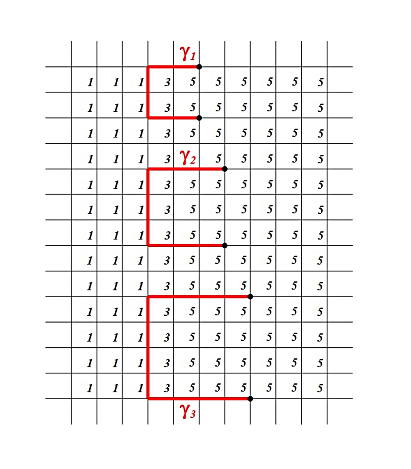
Refer to caption
Figure 4. Lengths of vertical edges in the metric dd on ℤ2\mathbb{Z}^{2}
  • •

    If x⩽0x\leqslant 0: d⁡((x,y),(x,y+1))=1d((x,y),(x,y+1))=1;

  • •

    If x=1x=1: d⁡((x,y),(x,y+1))=3d((x,y),(x,y+1))=3;

  • •

    If x⩾2x\geqslant 2: d⁡((x,y),(x,y+1))=5d((x,y),(x,y+1))=5.

Now consider a sequence {γn}\{\gamma_{n}\} of edge paths in (X,d)(X,d): for each n∈ℕn\in\mathbb{N}, define a path starting from an=(n+1,n+1)a_{n}=(n+1,n+1), which travels horizontally leftwards to (0,n+1)(0,n+1), then vertically down to (0,0)(0,0) and finally horizontally rightwards to bn=(n+1,0)b_{n}=(n+1,0). Again, see Figure 4.

It is easy to check that the paths γn\gamma_{n} are geodesic for all nn. We claim that (X,d,μ)(X,d,\mu) is a coarse median space. In fact, consider the identity map i​d:(X,d1,μ)→(X,d,μ)id:(X,d_{1},\mu)\rightarrow(X,d,\mu), where d1d_{1} is the edge-path metric defined by each edge having length 1. It is obvious that this is a bi-Lipschitz map and a median morphism, so (X,d,μ)(X,d,\mu) is indeed a coarse median space of rank 2. Now notice that [an,bn]={n+1}×[0,n+1][a_{n},b_{n}]=\{n+1\}\times[0,n+1]. So dH​(Im​γn,[an,bn])=n+1d_{H}(\mathrm{Im}\gamma_{n},[a_{n},b_{n}])=n+1, which implies there is no uniform bound on the Hausdorff distance between geodesics and intervals.

Unfortunately the space we have constructed is not geodesic, for instance the points (3,0),(3,1)(3,0),(3,1) are distance 55 apart, but there is no (integer) path of length less than 77 connecting them. We can modify the space easily to rectify this problem by subdividing the edges of length n>1n>1 by inserting n−1n-1 points declared to be unit distance apart as appropriate. The natural extension of the metric dd to include these points is now geodesic and we continue to denote it by dd. We are left with the issue of how to define coarse medians involving the inserted points. This is dealt with by projecting each point p=(x,y)p=(x,y) to its “floor” p¯=(x,⌊y⌋)\underline{p}=(x,\lfloor y\rfloor), the nearest original point to the vertex at or below it on a vertical line. We then define the ternary operator μ′\mu^{\prime} by μ′​(p,q,r)=μ⁡(p¯,q¯,r¯)\mu^{\prime}(p,q,r)=\mu(\underline{p},\underline{q},\underline{r}) when p,q,rp,q,r are distinct and if two are equal then we define μ′​(p,q,r)\mu^{\prime}(p,q,r) to be that point. Since the floor map moves points at most a distance of 44 in the dd metric, μ′\mu^{\prime} is still a coarse median operator with respect to the extended metric dd, and intervals between ana_{n} and bnb_{n} remain the same. ∎

References

  • [1] Hans-J Bandelt and Jarmila Hedlíková. Median algebras. Discrete mathematics, 45(1):1–30, 1983.
  • [2] Hans-Jurgen Bandelt and Victor Chepoi. Metric graph theory and geometry: a survey. Contemporary Mathematics, 453:49–86, 2008.
  • [3] Jason Behrstock, Mark Hagen, Alessandro Sisto, et al. Hierarchically hyperbolic spaces, I: Curve complexes for cubical groups. Geometry & Topology, 21(3):1731–1804, 2017.
  • [4] Jason Behrstock, Mark F Hagen, and Alessandro Sisto. Hierarchically hyperbolic spaces II: combination theorems and the distance formula. arXiv preprint arXiv:1509.00632, 2015.
  • [5] B. H. Bowditch. Coarse median spaces and groups. Pacific Journal of Mathematics, 261(1):53–93, 2013.
  • [6] B. H. Bowditch. Embedding median algebras in products of trees. Geometriae Dedicata, 170(1):157–176, 2014.
  • [7] M. R. Bridson and A. Ha¨\mathrm{\ddot{a}}fliger. Metric spaces of non-positive curvature, volume 319 of Grundlehren der Mathematischen Wissenschaften [Fundamental Principles of Mathematical Sciences]. Springer-Verlag, Berlin, 1999.
  • [8] I. Chatterji and G. A. Niblo. From wall spaces to CAT(0) cube complexes. International Journal of Algebra and Computation, 15(05n06):875–885, 2005.
  • [9] Indira Chatterji and Graham A Niblo. A characterization of hyperbolic spaces. Groups Geometry and Dynamics, 1(3):281, 2006.
  • [10] V. Chepoi. Graphs of some CAT(0) complexes. Advances in Applied Mathematics, 24(2):125–179, 2000.
  • [11] M. Gromov. Hyperbolic groups. In Essays in group theory, pages 75–263. Springer, 1987.
  • [12] J. R. Isbell. Median algebra. Transactions of the American Mathematical Society, 260(2):319–362, 1980.
  • [13] Milan Kolibiar and Tamara Marcisová. On a question of J. Hashimoto. Matematickỳ časopis, 24(2):179–185, 1974.
  • [14] G. A. Niblo and L. D. Reeves. The geometry of cube complexes and the complexity of their fundamental groups. Topology, 37(3):621–633, 1998.
  • [15] G.A. Niblo, N.J. Wright, and J. Zhang. The intrinsic geometry of coarse median spaces and their intervals. arXiv:1802.02499, 2018.
  • [16] B. Nica. Cubulating spaces with walls. Algebr. Geom. Topol, 4:297–309, 2004.
  • [17] Panos Papasoglu. Strongly geodesically automatic groups are hyperbolic. Inventiones mathematicae, 121(1):323–334, 1995.
  • [18] J. Pomroy. A characterisation of hyperbolic spaces. Master’s thesis, University of Warwick, 1994.
  • [19] M. Roller. Poc sets, median algebras and group actions. an extended study of Dunwoody’s construction and Sageev’s theorem. Southampton Preprint Archive, 1998.
  • [20] M. Sageev. Ends of group pairs and non-positively curved cube complexes. Proceedings of the London Mathematical Society, 3(3):585–617, 1995.
  • [21] Ján Špakula and Nick Wright. Coarse medians and property A. Algebraic & Geometric Topology, 17(4):2481–2498, 2017.
  • [22] Marcel L.J. van De Vel. Theory of convex structures, volume 50. Elsevier, 1993.
  • [23] R. Zeidler. Coarse median structures on groups. Master’s thesis, University of Vienna, Vienna, Austria, 2013.