$DD^{*}$ potentials in chiral effective field theory and possible molecular states

Chiral effective field theory (ChEFT) is an effective field theory respecting the chiral symmetry of Quantum chromodynamics (QCD) at low momenta. A prominent feature of ChEFT is that the results are expanded as a power series of small momenta rather than small coupling constants, which enables us to systematically study into the non-perturbative regime of the strong interaction. Pseudo-Goldstone bosons such as pion and kaon, with light masses, play very important roles for the low energy processes. Chiral symmetry constrains the form of the interaction quite strongly. Owing to the clear power counting scheme, ChEFT is very powerful to investigate the properties of light pseudoscalar bosons [1, 2, 3].

The situation becomes complicated when heavy hadrons involve. The power counting rule is broken because of large hadron masses. However, for the system with single heavy hadron and few light pseudoscalar bosons, the power counting scheme can be easily rebuilt, and many approaches of ChEFT have been developed to deal with the relevant scattering, interaction, electromagnetic moments, and other properties of such system. Heavy hadron chiral perturbation theory, the infrared regularization, and the extended-on-mass-shell scheme are frequently used in one heavy hadron sector [4, 5, 6, 7, 8, 9, 10, 11, 12, 13, 14, 15, 16, 17, 18]. Unfortunately, these approaches cannot be directly extended to study the properties about few heavy hadrons, like nuclear force.

Two-nucleon interaction bears another power counting problem. Two approximately on-shell nucleons in loop diagrams cause extra enhancement compared to the naive power counting, which prevents us from calculating scattering matrix directly. Weinberg proposed a framework to deal with the issue [19, 20]. One can first calculate an effective potential, i.e., sum of all two-particle irreducible (2PI) diagrams, and then iterate it with equations, such as Lippmann-Schwinger and Schrödinger equation, to retrieve two-particle reducible (2PR) contributions. The Weinberg’s formalism has been further extended and developed [21, 22, 23, 24, 27, 29, 30, 31, 32, 33, 34, 35]. For example, a unitary transformation is presented to remove the energy dependence of the potential in Refs. [23, 24]. The renormalization of potentials are carefully studied in Refs. [25, 26, 27, 28, 29]. The authors in Ref. [30] revisit the nucleon-nucleon potential up to NNNLO within ChEFT. In Refs. [31, 32], the nucleon-antinucleon potential is investigated within ChEFT. Very recently, a covariant formalism of the $N$-$N$ interaction is proposed in Ref. [33]. Three body and even four body nuclear forces have been systematically studied within ChEFT, see Refs. [34, 35] for a review. The application of ChEFT has been definitely advancing our understanding of the nuclear force [36].

With successes in the study of nuclear force, one may wonder whether ChEFT can help us to comprehend the interactions of heavy (charmed, bottomed) meson systems. Obviously, since heavy meson is heavier, we can make some assumptions such as the heavy quark limit without worries, and thus heavy hadron ChEFT is even more suitable than that in the nucleon system.

The $XYZ$ and similar exotic states have attracted a lot of interest in the hadron physics, and it is well known the interaction between heavy mesons is quite responsible for the strange behavior at close threshold in charmonium and bottomonium spectra (see Ref. [37] for a review). This starts with the discovery of the famous $X(3872)$, which was observed by the Belle Collaboration in $B$ decay process $B^{+-}\to K^{+-}\pi^{+}\pi^{-}J/\psi$ in 2003 [38]. $X(3872)$ is extremely close to the threshold of $D^{0}\bar{D}^{*0}$. Its mass is much smaller than quark model (such as the Godfrey-Isgur model [39]) predictions if it is regarded as $\chi^{\prime}_{c1}(2P)$ charmonium, and moreover it has a large decay width for the isospin violation process $X(3872)\to J/\psi\rho$. After that, more and more $XYZ$ and other exotic states candidates were discovered, such as recent observed pentaquark $P_{c}(4380)^{+}$ and $P_{c}(4450)^{+}$ [40] and still debated $X(5568)$ [41].

There are many models dealing with these states, such as the one-boson-exchange molecular model, some underlying multiquark models, kinematical effect, and so on (see the review [37]). For example, in Refs. [42, 43] $D^{*}_{(s)}\bar{D}^{*}_{(s)}$ and $D\bar{D}^{*}$ systems are studied within the local hidden gauge formalism to dynamically generate $Y(3940)$, $Z(3930)$, $X(4160)$ and $Z_{c}(3900)$. In Ref. [44], the authors have investigated the $D\bar{D}^{*}$ system and its relation to $Z_{c}(3900)$ using the covariant spectator theory. $Z_{c}(3900)$ is also studied from the pole counting rule [45]. The authors in Ref. [46] have discussed $D^{(*)}\bar{D}^{(*)}$ with the constituent quark models, and solved the four-body Schrödinger equation with the Gaussian expansion method. The contact interaction of $D\bar{D}^{*}$($B\bar{B}^{*}$) is specially investigated in Ref. [47] with the effective field theory, which is implemented with the heavy quark symmetry. The $D\bar{D}^{\ast}$ system is also intensively studied with different kinds of effective field theories, see Refs. [48, 49, 50, 51, 52, 55, 53, 54, 57, 56, 58] and many other works citied therein. For example, in Ref. [48], the authors studied the $D\bar{D}^{*}$ with XEFT using perturbative pions. In Ref [50], the authors studied $X(3872)$ and $D\bar{D}^{*}$ using non-perturbative pions. Moreover, the authors in Ref. [58] further included the effects of the $D^{*}$ width. In Ref. [59], the study of hadronic molecules with effective field theories are reviewed.

As mentioned above, there are many models dealing with heavy meson systems. Among them, the one-boson-exchange model has interpreted many exotic phenomenas and made some predictions which have been verified by the later discoveries of new particles at experiment. This model can provide the dynamical potentials of hadron systems, and then one can solve the Schrödinger equation to see if there is a bound state. The model has been widely used to study the interaction of the two-heavy-hadron systems and related exotic states. The research of the charmed-anticharmed system and $X(3872)$ experiences a long progress. It starts from the pion and $\sigma$ exchanges in early Ref. [60], directly extends to the multi-state exchanges [61], and then includes more complicated effects from $S$-$D$ mixing [62], isospin violation [63], and so on. For the investigation of nuclear force, after the boson exchange model develops for decades (see the discussion in Ref. [64]), ChEFT is applied at last and help us systematically build the modern system of knowledge. Following their steps, it is natural to introduce ChEFT into the study of heavy meson systems after the one-boson-exchange model.

There exist many works on heavy mesons system with one-boson-exchange model and effective field theories, as mentioned above. It is interesting to investigate their higher order effects in chiral effective field theory, and then discuss the potential in coordinate space and search for the bound state by solving Schrödinger equation. We will also compare the results with one-boson-exchange model.

In this work, we focus on the doubly charmed-meson system $DD^{*}$, which is clearer than the hidden charmed system for the absence of annihilation channels. It provides us another insight to understand the heavy-flavor dynamics and non-perturbative QCD. Furthermore, it is analogous to deuteron since they both have contact, one-pion exchange (OPE), and two-pion exchange (TPE) contributions without annihilation channels in our framework.

Till now, the only observed doubly heavy-flavor system is the $\Xi_{cc}^{++}$ baryon which was first discovered by SELEX collaboration [65]. Systems like $ccu$ and $ccd$ have been discussed a lot, and their properties such as masses and electromagnetic moments still need more efforts to get clarified [69, 71, 70, 72, 73, 74, 75, 76]. Very recently, LHCb group confirmed the existence of $\Xi_{cc}^{++}$ but disfavored the mass measured at SELEX [68]. With the technique and apparatus well developed nowadays, it is also possible to search for the doubly charmed boson made of $DD^{*}$ at experiment.

In Ref. [77], the authors studied $D^{(*)}D^{(*)}$($B^{(*)}B^{(*)}$) system to search for bound and resonant states, and they used pion and vector meson exchange potentials which are constrained by heavy quark symmetry and chiral symmetry. They found that in isospin 0 channel there exists a bound state in $S$-wave with binding energy $62.3$ MeV, and no bound state is found in isospin 1 with $S$-wave. In Ref. [78] the authors have studied $D^{(*)}D^{(*)}$ system using the one-boson-exchange model, and found that there exists a bound state consisting of $DD^{*}$ with binding energy $5\sim 43$ MeV in the isospin 0 channel. The authors in Ref. [79] investigate deuteron-like molecules with both open charm and bottom using the heavy-meson effective theory. In Ref. [80], charm-beauty meson bound states are dynamically generated from the $B^{(*)}D^{(*)}$ and $B^{(*)}\bar{D}^{(*)}$ interactions, and they also give the informations of the scattering lengths. There also exist lattice studies on $BB$ and $BB^{*}$ interaction [81, 82, 83]. Especially in Ref. [83], the authors considered both diquark-antidiquark and meson-meson configuration. In Ref. [84], we have investigated $\bar{B}\bar{B}$ interaction within heavy meson chiral effective field theory (HMChEFT). We obtain the potentials of the $\bar{B}\bar{B}$ system at one loop level, and have discussed the contact and two-pion exchange contributions in momentum space.

We investigate the $DD^{*}$ system in this work. As we mentioned before, we need to study the potentials first, and then access physical observables indirectly. Furthermore, the potential in coordinate space can give us more intuitive information about interaction between mesons, and we can further solve a dynamic equation to see whether there exists a hadronic molecule. This paper is organized as follows. After introduction, we elucidate the framework in Sec. II. In Sec. III, we give results of potentials in momentum space. In Sec. IV, we study the potential in coordinate space to search possible molecules. At last, we summarize our conclusions.

To study the $DD^{*}$ system under HMChEFT, we need to show Lagrangians and provide results systematically in a strict power counting scheme. Our results are arranged order by order with the small parameter $\epsilon=p/\Lambda_{\chi}$, where $p$ can be the momentum of pion, the residual momentum of heavy mesons, or the $D$-$D^{*}$ mass splitting, and $\Lambda_{\chi}$ represents either the chiral breaking scale or the mass of the heavy mesons. In this work, flavor SU(2) symmetry is always kept.

The effective potentials of $DD^{*}$ system receive contributions from the contact and OPE diagrams at the leading order $O(\epsilon^{0})$. At the next to leading order $O(\epsilon^{2})$, there are both tree and one-loop corrections. The effective potentials $\mathcal{V}$ are related to the Feynman amplitudes $\mathcal{M}$ of 2PI diagrams

which follows from the one-boson-exchange model despite some differences in conventions [91, 90].

At the lowest order $O(\epsilon^{0})$, there are two diagrams at tree level illustrated in Fig. 2. They represent the contact and OPE contributions, individually. The contact terms mainly affect the short range interaction between particles while the OPE contribution determines the behavior of the long range interaction.

With Lagrangians (1) and (5), the corresponding amplitudes can be easily computed. For the process $D(p_{1})D^{*}(p_{2})\to D(p_{3})D^{*}(p_{4})$ with isospin $I=1$, the amplitudes for diagrams (a) and (b) in Fig. 2 read

For the process $D(p_{1})D^{*}(p_{2})\to D(p_{3})D^{*}(p_{4})$ with $I=0$, the amplitudes are

In above equations, momentum $p=p_{1}-p_{4}$, the superscript $(0)$ denotes the order $O(\epsilon^{0})$, and the subscripts “$I=0,1$” stand for the process $DD^{*}\to DD^{*}$ with isospin $0,1$, respectively.

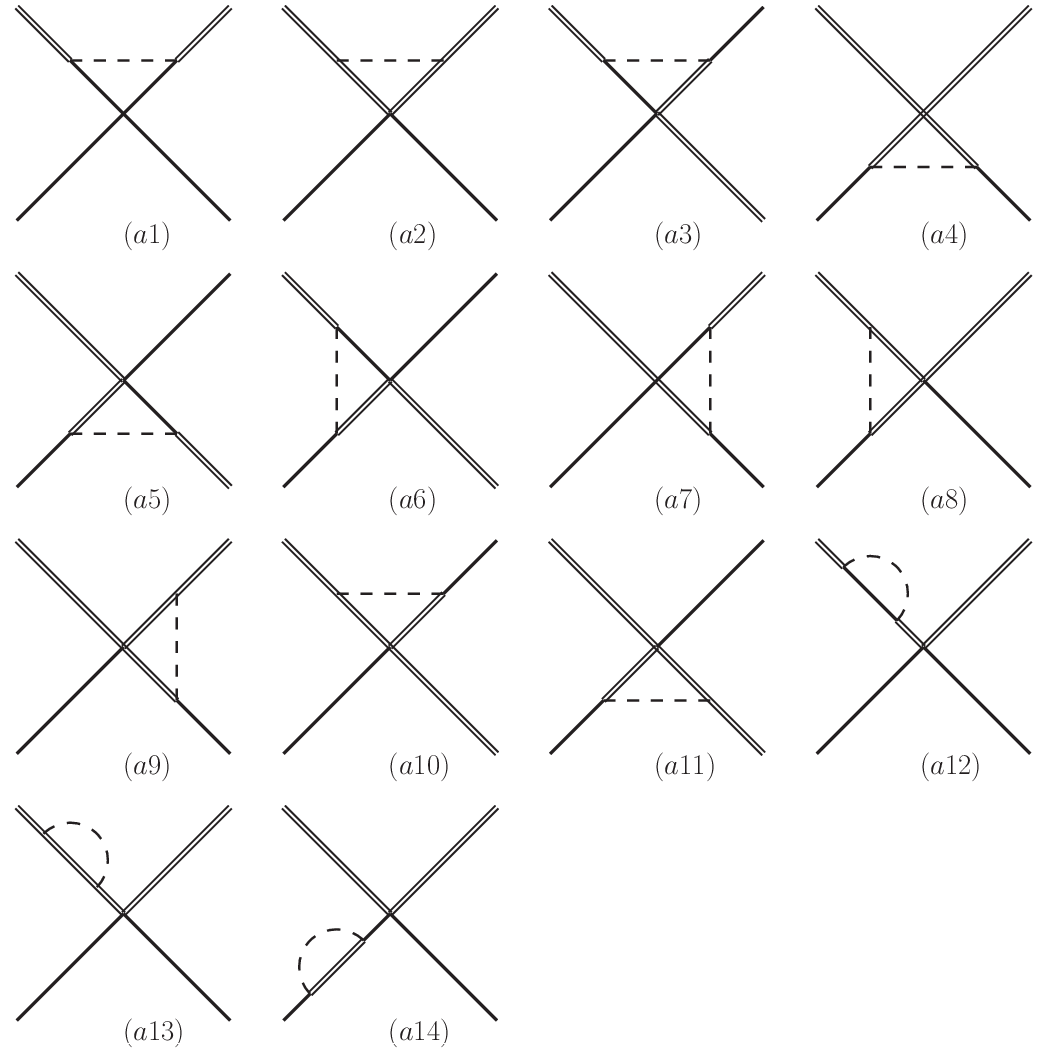
At $O(\epsilon^{2})$, a number of diagrams emerge. The tree diagrams at $O(\epsilon^{2})$ are similar to Fig. 2 (a), but the vertices should be replaced with those from Lagrangians (6-8). There are additionally three sets of one-loop diagrams.

The diagrams in the first set are for one-loop corrections to the contact terms. They are depicted in Fig. 3. Diagrams (a12)-(a12) represents contributions from the wave function renormalization of external legs.

We show the second set of diagrams in Fig. 4. They represent one-loop corrections to the OPE diagrams. The diagrams (b1)-(b6) and (b8)-(b9) in Fig. 4 contribute to the renormalization of the $DD^{*}\pi$ vertex. Therefore, we must use the value for the bare coupling $g$ in $\mathcal{M}^{(0)}$ at $O(\epsilon^{0})$ to avoid double counting. We show the relation between the bare coupling $g$ and the experiment coupling $g^{(2)}$ in Eq. (70) in Appendix B. Similarly, the bare decay constant $f$ should be used in Eqs. (13,15), too.

Final set is for the TPE diagrams which are illustrated in Fig. 5. They are important for the medium range interaction.

As discussed in the previous section, some diagrams, such as the box diagrams in Fig. 5, contain a 2PR part that should be subtracted. If there exists a loop function of a box diagram like

following Ref. [88, 84], we can separate the 2PR and 2PI parts by

The term proportional to Dirac $\delta$ function is just the 2PR part which should be dropped in potentials.

All the one-loop amplitudes of the diagrams Figs. 3-5 for the processes $DD^{*}\to DD^{*}$ are shown in Appendix A. The divergences of the loop functions are regularized with the dimensional regularization, and subtracted by the modified minimal subtraction scheme. Also, we list the definitions of the loop functions in Appendix C. The finite parts of the high order lagrangians should also contribute to tree level diagrams at $O(\epsilon^{2})$, and they are governed by a large number of LECs. However, it needs plenty of data for $D\bar{D}^{*}$ (or other channels such as $D\bar{D}$, $DD$) scattering in different partial waves to fit these LECs, but there is still lack now. Therefore in the present work, we only focus on the loop contributions at $O(\epsilon^{2})$.

We can easily obtain the potentials $\mathcal{V}_{I=1}^{DD^{*}}$ and $\mathcal{V}_{I=0}^{DD^{*}}$ from the Feynman amplitudes by multiplying a factor $-1/4$. The polarized vectors in the potentials are delicately dealt with in Ref. [89]. In this work, we only consider the $S$-wave interaction, which leads to the following substitutions in Eqs. (12)-(15), (34)-(66)

where we follow from the one-boson exchange model in Ref. [91, 90]. After all these procedures, the effective potentials $\mathcal{V}_{I=1}^{DD^{*}}$ and $\mathcal{V}_{I=0}^{DD^{*}}$ in the momentum space can be obtained. But, the potentials are energy dependent. A solution to this problem is proposed in Refs. [23, 24], where they apply a unitary transformation to get rid of the energy dependence. While in this work, we just take the transfered energies equal to zero, i.e. $p^{0}=0$ and $q^{0}=0$ for simplicity, as in the one-boson exchange model [60]. Also, we take the residual energies of the heavy mesons equal to zero, too.

We display input parameters for the numerical results: $m_{\pi}=0.139$ GeV, the mass difference $\delta=0.142$ GeV, $f_{\pi}=0.086$ GeV, and renormalization scale $\mu=4\pi f$. There are many works investigating the constant for $D^{(*)}D^{(*)}\pi$ coupling such as the lattice study [92, 93, 94], QCD sum rule [95, 96, 97, 98, 99], and other approaches [100, 101, 102]. The experimental process $D^{*}\to D\pi$ is fit to obtain the renormalized coupling $g^{(2)}$ [103], and we get the bare coupling $g=0.65$ by using the $O(\epsilon^{2})$ correction in Eq. (70).

First, we list the results for the contact contributions. For $\mathcal{V}_{I=1}^{DD^{*}}$ in the channel of isospin 1, the effective potential at $O(\epsilon^{0})$ and $O(\epsilon^{2})$ is as follows

And for the channel of isospin 0, we obtain

Obviously, the contact contributions are just constants, and they result in $\delta(r)$ potentials in coordinate space, which describes short distance effect. From Eqs. (20)-(23), we see the convergence of the series expansion is good. From Eqs. (21) and (23), the contact coupling constant $D_{a}$ does not appear in the effective potential at $O(\epsilon^{2})$ because the contributions from $D_{a}$ term are canceled among various diagrams in Fig. 3.

Next, we focus on the properties of the OPE and TPE contributions. We illustrate the corresponding potentials for channels with isospin 0 and 1 in Figs. 6 and 7, respectively, ranging from $q=|\mathbf{q}|=0$ to 300 MeV.

From Figs. 6 and 7, one can see that the OPE contributions at $O(\epsilon^{0})$ are dominant in both the $I=0$ and $I=1$ channels since the green dashed lines are close to the black solid ones. The OPE potentials at $O(\epsilon^{2})$ are small comparing to those at $O(\epsilon^{0})$. The sums of OPE contributions are negative from Figs. 6 and 7, which means the OPE interaction is attractive in both the $I=0$ and $I=1$ channels. We also notice that the OPE interaction in $I=0$ is more attractive than $I=1$.

The situation for the TPE potentials is more complicated. The TPE contributions behave differently in $I=0$ and $I=1$ channels. In Fig. 6, the TPE interaction for $I=0$ channel is attractive in the range $0\sim 300$ MeV, and it tends to grow beyond $300$ MeV. The TPE potential at $O(\epsilon^{2})$ is larger than the OPE one at $O(\epsilon^{0})$ in the range $0\sim 60$ MeV, while the OPE contribution exceeds that of TPE rapidly when $q$ is larger than 60 MeV, and becomes dominant. We can say that the convergence of the chiral series is good. Looking at Fig. 7, we see the TPE potential is repulsive in the range $0\sim 120$ MeV, while it becomes attractive as $q$ is beyond the range. The TPE potential at $O(\epsilon^{2})$ is smaller than the OPE contribution at $O(\epsilon^{0})$ in the lower range of the momentum, and becomes comparable in large momenta. It seems to indicate the convergence of the chiral series would be spoiled at larger transfered momenta. From the blue dot-dashed lines in Figs. 6 and 7, we see the TPE interaction in $I=1$ is more attractive than that in $I=0$.

Let us turn to the sum of these three contributions. The total contribution in Fig. 6 for $\mathcal{V}_{I=0}^{DD^{*}}$ is attractive, while in Fig. 7 for $\mathcal{V}_{I=1}^{DD^{*}}$ it is less attractive and tends to repulsive as $q$ becomes smaller than 50 MeV because of the repulsive TPE contribution. It makes us wonder whether there could form a bound state in the $DD^{*}$ system with the inclusion of contact contributions.

Although the pion exchange interaction is attractive at most momenta, there can still be no bound states if not attractive enough. Moreover, the contact interaction might be repulsive and furthermore decrease the possibility for the existence of a bound state. Thus the contact potentials must be first obtained numerically by the determination of the LECs. After that, we can investigate the effective potentials in coordinate space, and then solve the Schrödinger equation to search for possible molecular states.

In this work, we have systematically studied the $DD^{*}$ system with ChEFT. Due to the intrinsic difficulty of the ChEFT, we cannot obtain the physical observables directly from the Feynman diagrams. We alternatively calculate the potentials, i.e., the sum of all the 2PI diagrams, and then iterate them into Lippmann-Schwinger or Schrödinger equation to recover the 2PR contributions.

We have investigated the $DD^{*}$ effective potentials in ChEFT with Weinberg scheme. With the effective potentials obtained in momentum space, we have analyzed the contact, OPE and TPE contribution in detail. The OPE and TPE contributions are free of many LECs, and thus they are more model independent than the contact interaction since the LECs are determined with the resonance saturation model in this work. The OPE contribution at $O(\epsilon^{2})$ is smaller than that at $O(\epsilon^{0})$. The potential from TPE at $O(\epsilon^{2})$ is relatively large compared to that from OPE at $O(\epsilon^{0})$ in the $I=1$ channel, while it shows a good convergence in the $I=0$ channel. The TPE interaction is important and non-negligible.

We have determined the LECs in contact contributions with the resonance saturation model, and further explored the full potentials in coordinate space, which are regularized with a simple Gaussian cutoff. The roles of each contributions have been discussed, and the total potentials are very different in two channels. We have also discussed the importance of the contact contribution and the infulence of the cutoff in detail. Furthermore, we discuss the uncertainties of our approach, which comes from axial coupling $g$, LECs and truncation error. We find that the TPE contribution is non-negligible and attractive in general, while the contact contributions is an important element to compete the $\pi$-exchange contributions and cause quite different behavior in each channels. Despite the roughly estimated LECs, we notice that no bound state exists in the $I=1$ channel in a wide range of cutoff parameter, while there is a bound state in the $I=0$ channel as the cutoff is near $m_{\rho}$ in our approach. The binding energy is sensitive to the cutoff. Our results are consistent with those in the one-boson-exchange model [78].

In this work, we have ignored many other sub-leading effects from the isospin violation, $S$-$D$ mixing, recoiling, and so on. These effects can be investigated in future, and our framework shall be proved to be elegant.

We point out that the $DD^{*}$ molecule may be discovered at experiments through various processes. Since at Tevatron and LHCb there are a number of $B_{c}$ events, the $DD^{*}$ molecule can be produced via $B_{c}$ weak decay: singly Cabibbo-supressed process $B_{c}\to X(DD^{*})K$, doubly Cabibbo-supressed processes $B_{c}\to X(DD^{*})\pi$ and $B_{c}\to X(DD^{*})D$. Moreover we hope the $e^{+}e^{-}$ process such as $e^{+}e^{-}\to X(DD^{*})\bar{D}\bar{D}$ at BelleII can be studied to observe the state. The molecular states may be constructed through $DD$ final states. We also expect the lattice simulations to test our results.

References

• [1] S. Weinberg, Phenomenological Lagrangians, Physica A 96, 327 (1979).
• [2] J. Gasser and H. Leutwyler, Chiral Perturbation Theory to One Loop, Annals Phys. 158, 142 (1984).
• [3] S. Scherer and M. R. Schindler, A Primer for Chiral Perturbation Theory (Springer-Verlag, Berlin, 2012), Vol. 830, p. 1.
• [4] E. E. Jenkins and A. V. Manohar, Baryon chiral perturbation theory using a heavy fermion Lagrangian, Phys. Lett. B 255, 558 (1991).
• [5] V. Bernard, N. Kaiser, J. Kambor and U. G. Meissner, Chiral structure of the nucleon, Nucl. Phys. B 388, 315 (1992).
• [6] V. Bernard, N. Kaiser and U. G. Meissner, Chiral dynamics in nucleons and nuclei, Int. J. Mod. Phys. E 4, 193 (1995).
• [7] T. Becher and H. Leutwyler, Baryon chiral perturbation theory in manifestly Lorentz invariant form, Eur. Phys. J. C 9, 643 (1999).
• [8] T. Fuchs, J. Gegelia, G. Japaridze and S. Scherer, Renormalization of relativistic baryon chiral perturbation theory and power counting, Phys. Rev. D 68, 056005 (2003).
• [9] L. Geng, Recent developments in SU(3) covariant baryon chiral perturbation theory, Front. Phys. (Beijing) 8, 328 (2013).
• [10] F. K. Guo, C. Hanhart and U. G. Meissner, Interactions between heavy mesons and Goldstone bosons from chiral dynamics, Eur. Phys. J. A 40, 171 (2009).
• [11] Y. R. Liu, X. Liu and S. L. Zhu, Light Pseudoscalar Meson and Heavy Meson Scattering Lengths, Phys. Rev. D 79, 094026 (2009).
• [12] L. S. Geng, N. Kaiser, J. Martin-Camalich and W. Weise, Low-energy interactions of Nambu-Goldstone bosons with DD mesons in covariant chiral perturbation theory, Phys. Rev. D 82, 054022 (2010).
• [13] P. Wang and X. G. Wang, Study on 0+0^{+} states with open charm in unitarized heavy meson chiral approach, Phys. Rev. D 86, 014030 (2012).
• [14] M. Altenbuchinger, L.-S. Geng and W. Weise, Scattering lengths of Nambu-Goldstone bosons off DD mesons and dynamically generated heavy-light mesons, Phys. Rev. D 89, no. 1, 014026 (2014).
• [15] Z. H. Guo, U. G. Meißner and D. L. Yao, New insights into the Ds​0∗​(2317)D^{*}_{s0}(2317) and other charm scalar mesons, Phys. Rev. D 92, 094008 (2015).
• [16] D. L. Yao, M. L. Du, F. K. Guo and U. G. Meißner, One-loop analysis of the interactions between charmed mesons and Goldstone bosons, JHEP 1511, 058 (2015).
• [17] M. L. Du, F. K. Guo, U. G. Meißner and D. L. Yao, Study of open-charm 0+0^{+} states in unitarized chiral effective theory with one-loop potentials, arXiv:1703.10836 [hep-ph].
• [18] M. L. Du, F. K. Guo and U. G. Meissner, Subtraction of power counting breaking terms in chiral perturbation theory: spinless matter fields, JHEP 1610, 122 (2016).
• [19] S. Weinberg, Nuclear forces from chiral Lagrangians, Phys. Lett. B 251, 288 (1990).
• [20] S. Weinberg, Effective chiral Lagrangians for nucleon - pion interactions and nuclear forces, Nucl. Phys. B 363, 3 (1991).
• [21] C. Ordonez and U. van Kolck, Chiral lagrangians and nuclear forces, Phys. Lett. B 291, 459 (1992).
• [22] C. Ordonez, L. Ray and U. van Kolck, The Two nucleon potential from chiral Lagrangians, Phys. Rev. C 53, 2086 (1996).
• [23] E. Epelbaum, W. Gloeckle and U. G. Meissner, Nuclear forces from chiral Lagrangians using the method of unitary transformation. 1. Formalism, Nucl. Phys. A 637, 107 (1998).
• [24] E. Epelbaum, W. Gloeckle and U. G. Meissner, Nuclear forces from chiral Lagrangians using the method of unitary transformation. 2. The two nucleon system, Nucl. Phys. A 671, 295 (2000).
• [25] M. P. Valderrama, Perturbative renormalizability of chiral two pion exchange in nucleon-nucleon scattering, Phys. Rev. C 83, 024003 (2011).
• [26] M. Pavon Valderrama, Perturbative Renormalizability of Chiral Two Pion Exchange in Nucleon-Nucleon Scattering: P- and D-waves, Phys. Rev. C 84, 064002 (2011).
• [27] B. Long and C. J. Yang, Renormalizing chiral nuclear forces: a case study of P03{}^{3}P_{0}, Phys. Rev. C 84, 057001 (2011).
• [28] B. Long and C. J. Yang, Short-range nuclear forces in singlet channels, Phys. Rev. C 86, 024001 (2012).
• [29] B. Long and Y. Mei, Cutoff regulators in chiral nuclear effective field theory, Phys. Rev. C 93, no. 4, 044003 (2016).
• [30] E. Epelbaum, H. Krebs and U. G. Meißner, Improved chiral nucleon-nucleon potential up to next-to-next-to-next-to-leading order, Eur. Phys. J. A 51, no. 5, 53 (2015).
• [31] X. W. Kang, J. Haidenbauer and U. G. Meißner, Antinucleon-nucleon interaction in chiral effective field theory, JHEP 1402, 113 (2014).
• [32] L. Y. Dai, J. Haidenbauer and U. G. Meißner, Antinucleon-nucleon interaction at next-to-next-to-next-to-leading order in chiral effective field theory, arXiv:1702.02065 [nucl-th].
• [33] X. L. Ren, K. W. Li, L. S. Geng, B. W. Long, P. Ring and J. Meng, Leading order covariant chiral nucleon-nucleon interaction, arXiv:1611.08475 [nucl-th].
• [34] E. Epelbaum, H. W. Hammer and U. G. Meissner, Modern Theory of Nuclear Forces, Rev. Mod. Phys. 81, 1773 (2009).
• [35] R. Machleidt and D. R. Entem, Chiral effective field theory and nuclear forces, Phys. Rept. 503, 1 (2011).
• [36] U. G. Meissner, Phys. Scripta 91, no. 3, 033005 (2016)
• [37] H. X. Chen, W. Chen, X. Liu and S. L. Zhu, The hidden-charm pentaquark and tetraquark states, Phys. Rept. 639, 1 (2016).
• [38] S. K. Choi et al. [Belle Collaboration], Observation of a narrow charmonium-like state in exclusive B+(−)→K+(−)​π+​π−​J/ψB^{+(-)}\to K^{+(-)}\pi^{+}\pi^{-}J/\psi decays, Phys. Rev. Lett. 91, 262001 (2003).
• [39] S. Godfrey and N. Isgur, Mesons in a Relativized Quark Model with Chromodynamics, Phys. Rev. D 32, 189 (1985)..
• [40] R. Aaij et al. [LHCb Collaboration], Observation of J/ψ​pJ/\psi p Resonances Consistent with Pentaquark States in Λb0→J/ψ​K−​p\Lambda_{b}^{0}\to J/\psi K^{-}p Decays, Phys. Rev. Lett. 115, 072001 (2015).
• [41] V. M. Abazov et al. [D0 Collaboration], Evidence for a Bs0​π±B_{s}^{0}\pi^{\pm} state, Phys. Rev. Lett. 117, no. 2, 022003 (2016).
• [42] R. Molina and E. Oset, The Y⁡(3940)Y(3940), Z⁡(3930)Z(3930) and the X⁡(4160)X(4160) as dynamically generated resonances from the vector-vector interaction, Phys. Rev. D 80, 114013 (2009).
• [43] F. Aceti, M. Bayar, E. Oset, A. Martinez Torres, K. P. Khemchandani, J. M. Dias, F. S. Navarra and M. Nielsen, Prediction of an I=1I=1 D​D¯∗D\bar{D}^{*} state and relationship to the claimed Zc​(3900)Z_{c}(3900), Zc​(3885)Z_{c}(3885), Phys. Rev. D 90, no. 1, 016003 (2014).
• [44] J. He, The Zc​(3900)Z_{c}(3900) as a resonance from the D​D¯∗D\bar{D}^{*} interaction, Phys. Rev. D 92, no. 3, 034004 (2015).
• [45] Q. R. Gong, Z. H. Guo, C. Meng, G. Y. Tang, Y. F. Wang and H. Q. Zheng, Zc​(3900)Z_{c}(3900) as a D​D¯∗D\bar{D}^{*} molecule from the pole counting rule, Phys. Rev. D 94, no. 11, 114019 (2016). [arXiv:1604.08836 [hep-ph]].
• [46] Y. C. Yang, Z. Y. Tan, J. Ping and H. S. Zong, Possible D(∗)​D¯(∗)D^{(*)}\bar{D}^{(*)} and B(∗)​B¯(∗)B^{(*)}\bar{B}^{(*)} molecular states in the extended constituent quark models, arXiv:1703.09718 [hep-ph].
• [47] M. T. AlFiky, F. Gabbiani and A. A. Petrov, X(3872): Hadronic molecules in effective field theory, Phys. Lett. B 640, 238 (2006).
• [48] S. Fleming, M. Kusunoki, T. Mehen and U. van Kolck, Pion interactions in the X⁡(3872)X(3872), Phys. Rev. D 76, 034006 (2007).
• [49] S. Fleming and T. Mehen, Hadronic Decays of the X(3872) to chi(cJ) in Effective Field Theory, Phys. Rev. D 78, 094019 (2008).
• [50] V. Baru, A. A. Filin, C. Hanhart, Y. S. Kalashnikova, A. E. Kudryavtsev and A. V. Nefediev, Three-body D​D¯​πD\bar{D}\pi dynamics for the X⁡(3872)X(3872), Phys. Rev. D 84, 074029 (2011).
• [51] M. P. Valderrama, Power Counting and Perturbative One Pion Exchange in Heavy Meson Molecules, Phys. Rev. D 85, 114037 (2012).
• [52] J. Nieves and M. P. Valderrama, The Heavy Quark Spin Symmetry Partners of the X(3872), Phys. Rev. D 86, 056004 (2012).
• [53] C. Meng, J. J. Sanz-Cillero, M. Shi, D. L. Yao and H. Q. Zheng, Refined analysis on the X(3872) resonance, Phys. Rev. D 92, no. 3, 034020 (2015).
• [54] V. Baru, E. Epelbaum, A. A. Filin, J. Gegelia and A. V. Nefediev, Binding energy of the X⁡(3872)X(3872) at unphysical pion masses, Phys. Rev. D 92, no. 11, 114016 (2015).
• [55] V. Baru, E. Epelbaum, A. A. Filin, F.-K. Guo, H.-W. Hammer, C. Hanhart, U.-G. Meißner and A. V. Nefediev, Remarks on study of X(3872) from effective field theory with pion-exchange interaction, Phys. Rev. D 91, no. 3, 034002 (2015).
• [56] M. Jansen, H.-W. Hammer and Y. Jia, Finite volume corrections to the binding energy of the X⁡(3872)X(3872), Phys. Rev. D 92, no. 11, 114031 (2015).
• [57] E. Braaten, Galilean-invariant effective field theory for the X⁡(3872)X(3872), Phys. Rev. D 91, no. 11, 114007 (2015).
• [58] V. Baru, E. Epelbaum, A. A. Filin, C. Hanhart, U. G. Meissner and A. V. Nefediev, Heavy-quark spin symmetry partners of the X (3872) revisited, Phys. Lett. B 763, 20 (2016).
• [59] F. K. Guo, C. Hanhart, U. G. Meißner, Q. Wang, Q. Zhao and B. S. Zou, Hadronic molecules, arXiv:1705.00141 [hep-ph].
• [60] Y. R. Liu, X. Liu, W. Z. Deng and S. L. Zhu, Is X⁡(3872)X(3872) Really a Molecular State?, Eur. Phys. J. C 56, 63 (2008).
• [61] X. Liu, Z. G. Luo, Y. R. Liu and S. L. Zhu, X⁡(3872)X(3872) and Other Possible Heavy Molecular States, Eur. Phys. J. C 61, 411 (2009).
• [62] I. W. Lee, A. Faessler, T. Gutsche and V. E. Lyubovitskij, X⁡(3872)X(3872) as a molecular D​D∗DD^{*} state in a potential model, Phys. Rev. D 80, 094005 (2009).
• [63] N. Li and S. L. Zhu, Isospin breaking, Coupled-channel effects and Diagnosis of X⁡(3872)X(3872), Phys. Rev. D 86, 074022 (2012).
• [64] E. Epelbaum, U. G. Meissner, W. Gloeckle and C. Elster, Resonance saturation for four nucleon operators, Phys. Rev. C 65, 044001 (2002).
• [65] M. Mattson et al. [SELEX Collaboration], First observation of the doubly charmed baryon Ξc​c+\Xi^{+}_{cc}, Phys. Rev. Lett. 89, 112001 (2002).
• [66] B. Aubert et al. [BaBar Collaboration], Search for doubly charmed baryons Ξc​c+\Xi^{+}_{cc} and Ξc​c+⁣+\Xi^{++}_{cc} in BABAR, Phys. Rev. D 74, 011103 (2006).
• [67] R. Aaij et al. [LHCb Collaboration], Search for the doubly charmed baryon Ξc​c+\Xi_{cc}^{+}, JHEP 1312, 090 (2013).
• [68] R. Aaij et al. [LHCb Collaboration], Observation of the doubly charmed baryon Ξc​c+⁣+\Xi_{cc}^{++}, arXiv:1707.01621 [hep-ex].
• [69] Z. F. Sun, Z. W. Liu, X. Liu and S. L. Zhu, Masses and axial currents of the doubly charmed baryons, Phys. Rev. D 91, no. 9, 094030 (2015).
• [70] J. Hu and T. Mehen, Chiral Lagrangian with heavy quark-diquark symmetry, Phys. Rev. D 73, 054003 (2006).
• [71] F. S. Yu, H. Y. Jiang, R. H. Li, C. D. Lü, W. Wang and Z. X. Zhao, Discovery Potentials of Doubly Charmed Baryons, arXiv:1703.09086 [hep-ph].
• [72] H. X. Chen, W. Chen, X. Liu, Y. R. Liu and S. L. Zhu, A review of the open charm and open bottom systems, Rept. Prog. Phys. 80, no. 7, 076201 (2017).
• [73] H. X. Chen, Q. Mao, W. Chen, X. Liu and S. L. Zhu, Establishing low-lying doubly charmed baryons, arXiv:1707.01779 [hep-ph].
• [74] H. S. Li, L. Meng, Z. W. Liu and S. L. Zhu, Magnetic moments of the doubly charmed and bottomed baryons, arXiv:1707.02765 [hep-ph].
• [75] W. Wang, Z. P. Xing and J. Xu, Weak Decays of Doubly Heavy Baryons: SU(3) Analysis, arXiv:1707.06570 [hep-ph].
• [76] M. Karliner and J. L. Rosner, Quark-level analogue of nuclear fusion with doubly-heavy baryons, arXiv:1708.02547 [hep-ph].
• [77] S. Ohkoda, Y. Yamaguchi, S. Yasui, K. Sudoh and A. Hosaka, Exotic mesons with double charm and bottom flavor, Phys. Rev. D 86, 034019 (2012).
• [78] N. Li, Z. F. Sun, X. Liu and S. L. Zhu, Coupled-channel analysis of the possible D(∗)​D(∗),B¯(∗)​B¯(∗)D^{(*)}D^{(*)},\bar{B}^{(*)}\bar{B}^{(*)} and D(∗)​B¯(∗)D^{(*)}\bar{B}^{(*)} molecular states, Phys. Rev. D 88, 114008 (2013).
• [79] L. M. Abreu, Hadronic states with both open charm and bottom in effective field theory, Nucl. Phys. A 940, 1 (2015).
• [80] S. Sakai, L. Roca and E. Oset, Charm-beauty meson bound states from B⁡(B∗)​D​(D∗)B(B^{*})D(D^{*}) and B⁡(B∗)​D¯​(D¯∗)B(B^{*})\bar{D}(\bar{D}^{*}) interaction, arXiv:1704.02196 [hep-ph].
• [81] W. Detmold, K. Orginos and M. J. Savage, B​BBB Potentials in Quenched Lattice QCD, Phys. Rev. D 76, 114503 (2007).
• [82] P. Bicudo, K. Cichy, A. Peters and M. Wagner, B​BBB interactions with static bottom quarks from Lattice QCD, Phys. Rev. D 93, no. 3, 034501 (2016).
• [83] A. Francis, R. J. Hudspith, R. Lewis and K. Maltman, Lattice Prediction for Deeply Bound Doubly Heavy Tetraquarks, Phys. Rev. Lett. 118, no. 14, 142001 (2017).
• [84] Z. W. Liu, N. Li and S. L. Zhu, Chiral perturbation theory and the B¯​B¯\bar{B}\bar{B} strong interaction, Phys. Rev. D 89, 074015 (2014).
• [85] G. Burdman and J. F. Donoghue, Union of chiral and heavy quark symmetries, Phys. Lett. B 280, 287 (1992).
• [86] M. B. Wise, Chiral perturbation theory for hadrons containing a heavy quark, Phys. Rev. D 45, no. 7, R2188 (1992).
• [87] T. M. Yan, H. Y. Cheng, C. Y. Cheung, G. L. Lin, Y. C. Lin and H. L. Yu, Heavy quark symmetry and chiral dynamics, Phys. Rev. D 46, 1148 (1992), Erratum: [Phys. Rev. D 55, 5851 (1997)].
• [88] S. L. Zhu, C. M. Maekawa, B. R. Holstein, M. J. Ramsey-Musolf and U. van Kolck, Nuclear parity-violation in effective field theory, Nucl. Phys. A 748, 435 (2005).
• [89] D. Gülmez, U.-G. Meißner and J. A. Oller, A chiral covariant approach to ρ​ρ\rho\rho scattering, Eur. Phys. J. C 77 (2017) no.7, 460
• [90] Z. F. Sun, J. He, X. Liu, Z. G. Luo and S. L. Zhu, Zb​(10610)±Z_{b}(10610)^{\pm} and Zb​(10650)±Z_{b}(10650)^{\pm} as the B∗​B¯B^{*}\bar{B} and B∗​B¯∗B^{*}\bar{B}^{*} molecular states, Phys. Rev. D 84, 054002 (2011).
• [91] Z. F. Sun, Z. G. Luo, J. He, X. Liu and S. L. Zhu, A note on the B∗​B¯B^{*}\bar{B}, B∗​B¯∗B^{*}\bar{B}^{*}, D∗​D¯D^{*}\bar{D}, D∗​D¯∗D^{*}\bar{D}^{*}, molecular states, Chin. Phys. C 36, 194 (2012).
• [92] A. Abada, D. Becirevic, P. Boucaud, G. Herdoiza, J. P. Leroy, A. Le Yaouanc, O. Pene and J. Rodriguez-Quintero, First lattice QCD estimate of the gD∗​D​πg_{D^{*}D\pi} coupling, Phys. Rev. D 66, 074504 (2002).
• [93] D. Becirevic and F. Sanfilippo, Theoretical estimate of the D∗→D​πD^{*}\to D\pi decay rate, Phys. Lett. B 721, 94 (2013).
• [94] K. U. Can, G. Erkol, M. Oka, A. Ozpineci and T. T. Takahashi, Vector and axial-vector couplings of DD and D∗D^{*} mesons in 2+1 flavor Lattice QCD, Phys. Lett. B 719, 103 (2013).
• [95] P. Colangelo, G. Nardulli, A. Deandrea, N. Di Bartolomeo, R. Gatto and F. Feruglio, On the coupling of heavy mesons to pions in QCD, Phys. Lett. B 339, 151 (1994).
• [96] V. M. Belyaev, V. M. Braun, A. Khodjamirian and R. Ruckl, D∗​D​πD^{*}D\pi and B∗​B​πB^{*}B\pi couplings in QCD, Phys. Rev. D 51, 6177 (1995).
• [97] H. G. Dosch and S. Narison, B∗​B​πB^{*}B\pi couplings and D∗→D​πD^{*}\to D\pi decays within a 1/M1/M expansion in full QCD, Phys. Lett. B 368, 163 (1996).
• [98] P. Colangelo and F. De Fazio, QCD interactions of heavy mesons with pions by light cone sum rules, Eur. Phys. J. C 4, 503 (1998).
• [99] M. E. Bracco, M. Chiapparini, F. S. Navarra and M. Nielsen, Charm couplings and form factors in QCD sum rules, Prog. Part. Nucl. Phys. 67, 1019 (2012).
• [100] P. Colangelo, F. De Fazio and G. Nardulli, D∗D^{*} radiative decays and strong coupling of heavy mesons with soft pions in a QCD relativistic potential model, Phys. Lett. B 334, 175 (1994).
• [101] D. Becirevic and A. Le Yaouanc, G coupling (gB∗​B​πg_{B^{*}B\pi}, gD∗​D​πg_{D^{*}D\pi}): A Quark model with Dirac equation, JHEP 9903, 021 (1999).
• [102] B. El-Bennich, M. A. Ivanov and C. D. Roberts, Strong D∗→D​πD^{*}\to D\pi and B∗→B​πB^{*}\to B\pi couplings, Phys. Rev. C 83, 025205 (2011).
• [103] C. Patrignani et al. [Particle Data Group], Review of Particle Physics, Chin. Phys. C 40, no. 10, 100001 (2016).
• [104] G. Ecker, J. Gasser, A. Pich and E. de Rafael, The Role of Resonances in Chiral Perturbation Theory, Nucl. Phys. B 321, 311 (1989).
• [105] J. F. Donoghue, C. Ramirez and G. Valencia, The Spectrum of QCD and Chiral Lagrangians of the Strong and Weak Interactions, Phys. Rev. D 39, 1947 (1989).
• [106] V. Bernard, N. Kaiser and U. G. Meissner, Aspects of chiral pion - nucleon physics, Nucl. Phys. A 615, 483 (1997).
• [107] M. L. Du, F. K. Guo, U. G. Meissner and D. L. Yao, Aspects of the low-energy constants in the chiral Lagrangian for charmed mesons, Phys. Rev. D 94, no. 9, 094037 (2016).
• [108] J. X. Lu, L. S. Geng and M. P. Valderrama, Heavy Baryon Molecules in Effective Field Theory, arXiv:1706.02588 [hep-ph].
• [109] D. B. Kaplan, M. J. Savage and M. B. Wise, A New expansion for nucleon-nucleon interactions, Phys. Lett. B 424, 390 (1998).
• [110] J. Nieves, Renormalization of the one pion exchange N​NNN interaction in presence of derivative contact interactions, Phys. Lett. B 568, 109 (2003).
• [111] J. F. Yang and J. H. Huang, Renormalization of N​NNN scattering: Contact potential, Phys. Rev. C 71, 034001 (2005).
• [112] M. Pavon Valderrama and E. Ruiz Arriola, Renormalization of N​NNN interaction with chiral two pion exchange potential. central phases and the deuteron, Phys. Rev. C 74, 054001 (2006).
• [113] M. Pavon Valderrama and E. Ruiz Arriola, Renormalization of N​NNN interaction with chiral two pion exchange potential: Non-central phases, Phys. Rev. C 74, 064004 (2006), Erratum: Phys. Rev. C 75, 059905 (2007).
• [114] M. P. Valderrama, Power Counting and Wilsonian Renormalization in Nuclear Effective Field Theory, Int. J. Mod. Phys. E 25, no. 05, 1641007 (2016).
• [115] W. A. Bardeen, E. J. Eichten and C. T. Hill, Chiral multiplets of heavy - light mesons, Phys. Rev. D 68, 054024 (2003).