跳到论文正文
W Papers独立论文阅读器 arXiv:1708.06901 论文正文 计算阅读时间 · 0%
引用这篇论文根据当前论文元数据生成,正式投稿前建议核对。


License: arXiv.org perpetual non-exclusive license
arXiv:1708.06901v1 [cs.IT] 23 Aug 2017

Multi-Chart Detection Procedure for Bayesian Quickest Change-Point Detection with Unknown Post-Change Parameters

Jun Geng    Erhan Bayraktar    Lifeng Lai ††thanks: The work of J. Geng is supported by the National Natural Science Foundation of China under grant 61601144 and by the Fundamental Research Funds for the Central Universities under grant AUGA5710013915. The work of E. Bayraktar is supported in part by the NSF under grant number DMS-1613170 and in part by the Susan M. Smith Professorship. The work of L. Lai is supported by the National Science Foundation under grants CNS-1660128 and ECCS-1711468. This paper was presented in part at IEEE International Conference on Acoustics, Speech, and Signal Processing (ICASSP), Shanghai, China, Mar. 2016˜[1]. J. Geng is with the School of Electronics and Information Engineering, Harbin Institute of Technology, Harbin, 150001, China (Email: jgeng@hit.edu.cn). E. Bayraktar is with the Department of Mathematics, University of Michigan, Ann Arbor, MI 48109, USA (Email:erhan@umich.edu). L. Lai is with the Department of Electrical and Computer Engineering, University of California, Davis, CA, 95616, USA (Email: lflai@ucdavis.edu).
Abstract

In this paper, the problem of quickly detecting an abrupt change on a stochastic process under Bayesian framework is considered. Different from the classic Bayesian quickest change-point detection problem, this paper considers the case where there is uncertainty about the post-change distribution. Specifically, the observer only knows that the post-change distribution belongs to a parametric distribution family but he does not know the true value of the post-change parameter. In this scenario, we propose two multi-chart detection procedures, termed as M-SR procedure and modified M-SR procedure respectively, and show that these two procedures are asymptotically optimal when the post-change parameter belongs to a finite set and are asymptotically ϵ−\epsilon-optimal when the post-change parameter belongs to a compact set with finite measure. Both algorithms can be calculated efficiently as their detection statistics can be updated recursively. We then extend the study to consider the multi-source monitoring problem with unknown post-change parameters. When those monitored sources are mutually independent, we propose a window-based modified M-SR detection procedure and show that the proposed detection method is first-order asymptotically optimal when post-change parameters belong to finite sets. We show that both computation and space complexities of the proposed algorithm increase only linearly with respect to the number of sources.

I Introduction

To quickly detect the abrupt or the abnormal change in the observing sequence is of interest in wide range of practical applications. For example, in the cognitive radio system, the secondary user wants to quickly identify the time instant when the primary user accesses or releases the channel to maximize its throughput [2, 3, 4]. As another example, in seismic monitoring, it is crucial to quickly detect the abnormal signal caused by the earth crust movement. In such applications, to minimize the detection delay, which is the difference between the time when the abnormal change occurs and the time when the change is declared, is of interest. Quickest change-point detection (QCD) is a suitable mathematical framework for such applications. In particular, QCD aims to design online algorithms that can identify the abrupt change in the probabilistic distribution of a stochastic process as quickly and accurately as possible. QCD has two main classes of problem formulations: Bayesian formulation [5, 6] and non-Baysian formulation [7, 8]. For the classic Bayesian formulation, one sequentially observes a stochastic process {Xk}k=1∞\{X_{k}\}_{k=1}^{\infty} with a random change-point tt. Before the change-point tt, the sequence X1,…,Xt−1X_{1},\ldots,X_{t-1} are independent and identically distributed (i.i.d.) with probability density function (pdf) f0f_{0}, and after tt, the sequence Xt,Xt+1,…X_{t},X_{t+1},\ldots are i.i.d. with pdf f1f_{1}. In the Bayesian formulation, the change-point tt is typically modeled as a geometrically distributed random variable. The goal is to find an optimal stopping time τ\tau, at which we declare the change has happened, that minimizes the average detection delay 𝔼⁡[(τ−t)+]\mathbb{E}[(\tau-t)^{+}] subjected to a false alarm constraint. The Shiryaev-Robert (SR) procedure is known to be the optimal detection procedure for Bayesian QCD [6, 9]. In the non-Bayesian formulation, the change-point tt is assumed to be a fixed but unknown constant.

In the classic Bayesian QCD, it assumes that both the pre-change distribution f0f_{0} and the post-change distribution f1f_{1} are perfectly known by the observer. In most of practical applications, it is reasonable to assume that the pre-change distribution is known, as we typically know the behavior of the system in the normal state. However, one may not know the post-change distribution perfectly, as this represents the system in the abnormal states. Motivated by this fact, in this paper we extend the classic Bayesian QCD problem to the case with incomplete post-change information. In particular, we focus on the case that the post-change distribution belongs to a parametric distribution family, but the true post-change parameter, which belongs to a known compact set Λ\Lambda, is unknown to the observer. The goal of the observer is to design an effective online algorithm to quickly detect the change-point in the observation sequence for all possible post-change parameter in Λ\Lambda. In this scenario, we propose two low complexity multi-chart procedures for the purpose of quickest detection. In the first proposed detection algorithm, the observer divides Λ\Lambda into II small disjoint subsets. By selecting one candidate point in each small subset, the observer constructs a finite set ΛD⊆Λ\Lambda_{D}\subseteq\Lambda. Then, for each elements within ΛD\Lambda_{D}, the observer runs a SR detection procedure; the observer declares that the change has occurred when any one of these procedures stops. We note that the observer runs multiple SR procedures simultaneously in each time slot, we term this algorithm as M-SR procedure. The second proposed algorithm is similar to the first one except that it replaces the summation operator within the SR statistic by the maximum operator; hence we term the second proposed multi-chart procedure as the modified M-SR procedure. For both proposed algorithms, we show that they are asymptotically optimal for the post-change parameters within ΛD\Lambda_{D} and asymptotically ϵ−\epsilon-optimal for all parameters within Λ\Lambda if ΛD\Lambda_{D} is properly selected. The definition of asymptotic ϵ−\epsilon-optimality will be given explicitly in the sequel. Loosely speaking, it indicates that the performance loss of the proposed algorithm is no larger than a small constant ϵ\epsilon as the false alarm probability vanishes. We further point out that both proposed algorithms can be calculated recursively hence they are computationally efficient.

We then further extend the study to the multi-source monitoring problem under Bayesian QCD framework. In particular, the observer monitors LL mutually independent sources (except the change happens at the same time) and aims to detect the geometrically distributed change-point tt as quickly as possible. We consider the case that the distributions of all LL sources change simultaneously at tt but the post-change distribution of each source contains one unknown parameter. If we directly apply the M-SR or the modified M-SR procedure to the case of multi-variate unknown parameter, the computational complexity will increase exponentially w.r.t. LL. In this scenario, we propose a window-based modified M-SR procedure. We analyze the complexity and the performance of the proposed algorithm in detail, and show that the computational complexity of this proposed algorithm increases only linearly w.r.t. LL and the proposed algorithm is asymptotically optimal as the false alarm probability goes to zero.

The problem considered in this paper is related to recent works on the QCD problem that take the unknown post-change parameter into consideration. Due to limited space, we mention a few of them. For Bayesian setups, optimal solutions are likely to be obtained by converting proposed problems into Markovian optimal stopping problems. For example, [10] solves the Poisson disorder problem with unknown post-change arrival rate; [11] solves the Bayesian sequential change diagnosis problem, in which the observer aims not only to quickly detect the change but also to accurately identify the post-change parameter from a finite set; [12] solves a generalized formulation of the sequential change diagnosis problem for a Markov modulated sequence. For non-Bayeisan QCD setups, most of existing works propose modified versions of the CUSUM detection procedure, which is the optimal scheme for the classic non-Bayeisan QCD problem with known parameters [13], and discuss their robustness over the post-change uncertainty. For example, [7, 14, 15] replace the unknown likelihood ratio in the CUSUM statistic by the generalized likelihood ratio (GLR). [16] proposes the mixture-based CUSUM algorithm in which the CUSUM statistic is averaged over a prior distribution of the unknown parameter. [17] further shows the asymptotic optimality of the GLR-based CUSUM and the mixture-based CUSUM detection algorithms. [18] designs a composite stopping time that combines multiple CUSUM procedures to quickly detect the disorder time in the Wiener process with post-change uncertainty. [19] mentions the multi-chart CUSUM detection strategy. One may refer to a recent book [20] and references therein for more detailed results of this topic.

Different from aforementioned literatures, our work is formulated under Bayesian framework and focuses on the performance of low complexity multi-chart detection procedures instead of optimal schemes, which usually have high computational complexities. [21] has studied the asymptotic detection rules for Bayesian sequential diagnosis problem. Our paper focuses on the QCD problem and shows that the multi-chart version of the well-known SR procedure exhibits robustness over unknown parameters. The problem studied in this paper can be also viewed as a special case of the Markov chain tracking problem [22, 23, 24] with several absorbing states. However, those works focus on the optimal solution of generalized formulations while our work focus on the asymptotic optimal algorithms for the QCD problem.

There are also many recent works considering the QCD problem for multi-source monitoring. [25] is one of the most related works. Specifically, [25] considers the QCD problem in a distributed multi-sensor system when the post-change parameters are unknown. Authors also proposed to use multi-chart CUSUM to solve the proposed problem. In addition, [26] proposes the SUM algorithm, which is based on the sum of local CUSUMs, to quickly detect the abrupt change in multiple independent data streams. However, [26] only focuses on the case with known post-change distributions. Both [25] and [26] are formulated under non-Bayesian setting. We consider the multi-source monitoring problem under Bayesian QCD framework and discuss the performance and the implementation complexity of the proposed algorithm in detail.

This paper extends our previous conference publication [1] in several ways. Specifically, [1] only discusses the asymptotic optimality of the M-SR procedure when the post-change parameter belongs to a finite set. In addition to including the contributions made in [1], this paper also proposes the modified M-SR procedure, and studies the performance of both algorithms under a more general setting. Furthermore, we consider the multi-source monitoring problem and analyze the performance of our newly proposed algorithm.

The remainder of this paper is organized as follows. The mathematic model is given in Section II. Section III presents the proposed multi-chart detection algorithms and analyzes their asymptotic performances. Section IV discusses the multi-source monitoring problem and analyzes the performance of the proposed window-based modified M-SR procedure. Technical proofs in this paper are presented in Section V. Numerical examples are given in Section VI to illustrate the theoretic results obtained in this work. Finally, Section VII offers concluding remarks.

II Model

II-A Problem Formulation

We consider a random observation sequence {Xk,k=1,2,…}\left\{X_{k},k=1,2,\ldots\right\} whose distribution changes at an unknown time tt. In particular, observations obtained before the change-point tt, namely X1,X2,…,Xt−1X_{1},X_{2},\ldots,X_{t-1}, are i.i.d. with pdf g⁡(x,θ0)g(x;\theta_{0}); observations obtained after the change-point tt, namely Xt,Xt+1,…X_{t},X_{t+1},\ldots, are i.i.d. with pdf f⁡(x,λ)f(x;\lambda).

In the classic QCD problem, both the pre-change distribution g⁡(x,θ0)g(x;\theta_{0}) and the post-change distribution f⁡(x,λ)f(x;\lambda) are perfectly known by the observer. In this paper, we consider the case that the observer only knows partial information of the post-change distribution. Specifically, we assume that the pre-change distribution g⁡(x,θ0)g(x;\theta_{0}) is perfectly known to the observer; hence θ0\theta_{0} is a known parameter. However, the post-change distribution f⁡(x,λ)f(x;\lambda) contains an unknown parameter λ\lambda. The observer knows that λ\lambda is taken from a compact set Λ\Lambda but he does not know the true value of λ\lambda. For notation convenience, in the rest of paper, g⁡(x,θ0)g(x,\theta_{0}) is also denoted as gθ0​(x)g_{\theta_{0}}(x), and f⁡(x,λ)f(x;\lambda) is denoted as fλ​(x)f_{\lambda}(x).

In this paper, we focus on the Bayesian QCD problem. In Bayesian framework, the change-point tt is modeled as a geometric random variable with known parameter ρ\rho, i.e., for 0<ρ<10<\rho<1,

P(t=k)=ρ(1−ρ)k−1,k=1,2,….\displaystyle P(t=k)=\rho(1-\rho)^{k-1},\quad k=1,2,\ldots. (1)

Observations XkX_{k}’s generate the filtration {ℱk}k∈ℕ\{\mathcal{F}_{k}\}_{k\in\mathbb{N}} with

ℱk=σ(X1,⋯,Xk),k=1,2,…,\mathcal{F}_{k}=\sigma(X_{1},\cdots,X_{k}),\quad k=1,2,\ldots,

and ℱ0\mathcal{F}_{0} contains the sample space Ω\Omega.

To facilitate the presentation, we denote Pk(θ0,λi)P_{k}^{(\theta_{0},\lambda_{i})} as the conditional probability measure of the observation sequence given {t=k;λ=λi}\{t=k;\lambda=\lambda_{i}\}. For a measurable event FF, we define probability measure Pπ(θ0,λi)P_{\pi}^{(\theta_{0},\lambda_{i})} as

Pπ(θ0,λi)​(F):=∑k=1∞Pk(θ0,λi)​(F)​P​(t=k).\displaystyle P_{\pi}^{(\theta_{0},\lambda_{i})}(F):=\sum_{k=1}^{\infty}P_{k}^{(\theta_{0},\lambda_{i})}(F)P(t=k).

We use 𝔼k(θ0,λi)\mathbb{E}_{k}^{(\theta_{0},\lambda_{i})} and 𝔼π(θ0,λi)\mathbb{E}_{\pi}^{(\theta_{0},\lambda_{i})} to denote the expectations with respect to probability measures Pk(θ0,λi)P_{k}^{(\theta_{0},\lambda_{i})} and Pπ(θ0,λi)P_{\pi}^{(\theta_{0},\lambda_{i})}, respectively.

The observer aims to detect the change-point as quickly and accurately as possible. Let 𝒯\mathcal{T} be a set of finite stopping times adapted to ℱk\mathcal{F}_{k}. A stopping time τ∈𝒯\tau\in\mathcal{T} indicates the time instant that the observer stops taking observation and declares that the change has occurred. If the observer raises the alarm before the change-point occurs, i.e. τ<t\tau<t, we call the observer makes a false alarm. On the other hand, if τ≥t\tau\geq t, we define (τ−t)(\tau-t) as the detection delay. Hence, we use the following two performance metrics to evaluate a detection procedure τ\tau:

ADD⁡(τ,θ0,λ):=𝔼π(θ0,λ)​[(τ−t)+],\displaystyle\mathrm{ADD}(\tau;\theta_{0},\lambda):=\mathbb{E}_{\pi}^{(\theta_{0},\lambda)}[(\tau-t)^{+}],
PFA⁡(τ,θ0,λ):=Pπ(θ0,λ)​(τ<t).\displaystyle\mathrm{PFA}(\tau;\theta_{0},\lambda):=P_{\pi}^{(\theta_{0},\lambda)}(\tau<t).

In our setup, the observer aims to minimize the average detection delay (ADD) while keeping the probability of false alarm (PFA) under control regardless of the value of λ\lambda. In other words, the observer wants to solve the following optimization problem:

infτ∈𝒯ADD⁡(τ,θ0,λ) for all ​λ∈Λ,\displaystyle\inf_{\tau\in\mathcal{T}}\mathrm{ADD}(\tau;\theta_{0},\lambda)\quad\text{ for all }\lambda\in\Lambda,
subject to ​supλ∈ΛPFA⁡(τ,θ0,λ)≤α,\displaystyle\textrm{subject to }\sup_{\lambda\in\Lambda}\mathrm{PFA}(\tau;\theta_{0},\lambda)\leq\alpha, (2)

where α\alpha is a constant to control the false alarm. We note that (2) aims to minimize ADD and to achieve a small probability of false alarm for all possible post-change parameters simultaneously. In general, it is difficult to find an optimal solution for the above multi-objective optimization problem. In this paper, we aim to design asymptotically optimal or sub-optimal detection algorithms.

II-B Other Related Formulations

We emphasize that, in our formulation stated in (2), the observer requires no prior distribution of λ∈Λ\lambda\in\Lambda. In some existing related literatures, such as [10, 18, 21], the prior distribution of the post-change parameter is assumed to be known by the observer. When the prior distribution of Λ\Lambda is available, in our context, it is natural to consider the problem formulation with averaged or weighted performance metrics.

Specifically, let G⁡(λ)G(\lambda) be the prior distribution (or a subjective normalized weighting function) of Λ\Lambda, and

∫λ∈Λd​G​(λ)=1.\displaystyle\int_{\lambda\in\Lambda}dG(\lambda)=1. (3)

In this case, we can define an averaged PFA as

Pπ,ω(θ0)​(τ<t):=∫λ∈ΛPπ(θ0,λ)​(τ<t)​𝑑G​(λ),\displaystyle P_{\pi,\omega}^{(\theta_{0})}(\tau<t):=\int_{\lambda\in\Lambda}P_{\pi}^{(\theta_{0},\lambda)}(\tau<t)dG(\lambda), (4)

and define an averaged ADD as

𝔼π,ω(θ0)​[(τ−t)+]:=∫λ∈Λ𝔼π(θ0,λ)​[(τ−t)+]​𝑑G​(λ).\displaystyle\mathbb{E}_{\pi,\omega}^{(\theta_{0})}[(\tau-t)^{+}]:=\int_{\lambda\in\Lambda}\mathbb{E}_{\pi}^{(\theta_{0},\lambda)}[(\tau-t)^{+}]dG(\lambda). (5)

Correspondingly, the observer may want to solve the following optimization problem

infτ∈𝒯𝔼π,ω(θ0)​[(τ−t)+],\displaystyle\inf_{\tau\in\mathcal{T}}\mathbb{E}_{\pi,\omega}^{(\theta_{0})}[(\tau-t)^{+}],
subject to ​Pπ,ω(θ0)​(τ<t)≤α.\displaystyle\textrm{subject to }P_{\pi,\omega}^{(\theta_{0})}(\tau<t)\leq\alpha. (6)

We note that the (asymptotically) optimal solution of Formulation (2) is also (asymptotically) optimal for Formulation (6). To see this fact, it is worth to notice that

Pπ(θ0,λi)​(τ<t)=Pπ(θ0,λj)​(τ<t)∀λi,λj∈Λ,λi≠λj.P_{\pi}^{(\theta_{0},\lambda_{i})}(\tau<t)=P_{\pi}^{(\theta_{0},\lambda_{j})}(\tau<t)\quad\forall\lambda_{i},\lambda_{j}\in\Lambda,\lambda_{i}\neq\lambda_{j}.

This is because all observations are generated from gθ0​(x)g_{\theta_{0}}(x) on the event {τ<t}\{\tau<t\} (when false alarm happens); hence the false alarm probability is independent of the post-change parameter λ\lambda. As a result, we have

Pπ,ω(θ0)​(τ<t)=Pπ(θ0,λi)​(τ<t)=supλPπ(θ0,λ)​(τ<t).\displaystyle P_{\pi,\omega}^{(\theta_{0})}(\tau<t)=P_{\pi}^{(\theta_{0},\lambda_{i})}(\tau<t)=\sup_{\lambda}P_{\pi}^{(\theta_{0},\lambda)}(\tau<t). (7)

Hence, if the worst case false alarm constraint in (2) is satisfied by detection procedure τ\tau, the average false alarm constraint in (6) is also satisfied. Furthermore, for the objective function, we note that to minimize ADD​(τ,θ0,λ)\textrm{ADD}(\tau;\theta_{0},\lambda) for all λ∈Λ\lambda\in\Lambda simultaneously in (2) is stronger than to minimize 𝔼π,ω(θ0)​[(τ−t)+]\mathbb{E}_{\pi,\omega}^{(\theta_{0})}[(\tau-t)^{+}], the detection delay averaged over λ\lambda, in (5). Hence, Formulation (2) is more stringent than Formulation (6). As a result, the (asymptotically) optimal solution for Formulation (2) is also expected to have a good performance for Formulation (6).

III Multi-Chart Procedures and Their Sub-Optimality

It is well known that the SR procedure is the optimal detection procedure for classic Bayesian QCD problem. In this section, we propose two new detection algorithms, both of which are modified versions of the SR procedure, and analyze their performances.

III-A Multi-chart procedures

For the classic Bayesian QCD problem with pre-change distribution f0f_{0} and post-change distribution f1f_{1}, the SR procedure is known as

Rn:=∑k=1n∏q=kn11−ρ​f1​(Xq)f0​(Xq),\displaystyle R_{n}:=\sum_{k=1}^{n}\prod_{q=k}^{n}\frac{1}{1-\rho}\frac{f_{1}(X_{q})}{f_{{0}}(X_{q})},
τS​R:=inf{n≥1:log⁡Rn>log⁡B},\displaystyle\tau_{SR}:=\inf\left\{n\geq 1:\log R_{n}>\log B\right\},

for a properly chosen threshold BB. For our formation, as the post-change distribution contains an unknown parameter, it is natural to consider replacing the likelihood ratio in the SR procedure with the generalized likelihood ratio. In our context, the GLR-based SR procedure can be written as

Rn∗:=supλ∈Λ∑k=1n∏q=kn11−ρ​fλ​(Xq)gθ0​(Xq),\displaystyle R_{n}^{*}:=\sup_{\lambda\in\Lambda}\sum_{k=1}^{n}\prod_{q=k}^{n}\frac{1}{1-\rho}\frac{f_{\lambda}(X_{q})}{g_{\theta_{0}}(X_{q})},
τG​L​R:=inf{n≥1:log⁡Rn∗>log⁡B}.\displaystyle\tau_{GLR}:=\inf\left\{n\geq 1:\log R_{n}^{*}>\log B\right\}.

Though the GLR-based SR procedure is natural and attractive, it has several shortcomings. Theoretically, it is a challenging task to find the false alarm probability of τG​L​R\tau_{GLR}. Practically, τG​L​R\tau_{GLR} has large computational complexity as the observer needs to solve for the best λ∗\lambda^{*} at each time slot nn. The computational complexity depends on the specific form of gθ0g_{\theta_{0}} and fλf_{\lambda}, which could lead to very challenging optimization problems.

In order to resolve these difficulties, we discretize the feasible set Λ\Lambda by selecting finitely many candidate points. Specifically, let ΛD={λ0,λ1,…,λI−1}\Lambda_{D}=\{\lambda_{0},\lambda_{1},\ldots,\lambda_{I-1}\} be a discrete set with II different elements, and ΛD⊆Λ\Lambda_{D}\subseteq\Lambda. For i=0,…,I−1i=0,\ldots,I-1, let

Rn(θ0,λi):=∑k=1n∏q=kn11−ρ​fλi​(Xq)gθ0​(Xq)\displaystyle R_{n}^{(\theta_{0},\lambda_{i})}:=\sum_{k=1}^{n}\prod_{q=k}^{n}\frac{1}{1-\rho}\frac{f_{\lambda_{i}}(X_{q})}{g_{\theta_{0}}(X_{q})} (8)

be the detection statistic, we propose the following detection procedure:

τR(i)=inf{n≥1:log⁡Rn(θ0,λi)>log⁡Bi},\displaystyle\tau_{R}^{(i)}=\inf\left\{n\geq 1:\log R_{n}^{(\theta_{0},\lambda_{i})}>\log B_{i}\right\}, (9)
τR=mini∈{0,…,I−1}⁡τR(i).\displaystyle\tau_{R}=\min_{i\in\{0,\ldots,I-1\}}\tau_{R}^{(i)}. (10)

There are a few comments about the proposed algorithm. Firstly, the proposed algorithm can be viewed as a GLR-based SR detection procedure over the discrete set ΛD\Lambda_{D}. As we use ΛD\Lambda_{D} to approximate the post-change parameter set, τR\tau_{R} then can be viewed as an approximation of τG​L​R\tau_{GLR}. Secondly, the proposed algorithm is a multi-chart detection procedure. Specifically, in the proposed algorithm, the observer updates II statistics Rn(θ0,λi)R_{n}^{(\theta_{0},\lambda_{i})}, i=0,…,I−1i=0,\ldots,I-1, in a parallel manner at each time slot, and each statistic is compared with its own threshold BiB_{i}. The procedure stops when any one of statistics exceeds its corresponding threshold. As Rn(θ0,λi)R_{n}^{(\theta_{0},\lambda_{i})} is the statistic used in the SR procedure, we term our proposed multi-chart procedure as M-SR procedure. Thirdly, we comment that τR\tau_{R} can be calculated efficiently since Rn(θ0,λi)R_{n}^{(\theta_{0},\lambda_{i})} can be updated recursively at each time slot. It is easy to see

Rn(θ0,λi)=(1+Rn−1(θ0,λi))​11−ρ​fλi​(Xn)gθ0​(Xn).\displaystyle R_{n}^{(\theta_{0},\lambda_{i})}=\left(1+R_{n-1}^{(\theta_{0},\lambda_{i})}\right)\frac{1}{1-\rho}\frac{f_{\lambda_{i}}(X_{n})}{g_{\theta_{0}}(X_{n})}. (11)

Hence, the computational complexity of the proposed M-SR procedure is on the order of O⁡(I)O(I) at each time slot.

Besides the M-SR procedure, we also propose the following modified M-SR procedure:

Cn(θ0,λi):=max1≤k≤n∏q=kn11−ρfλi​(Xq)gθ0​(Xq),i=0,…,I−1,\displaystyle C_{n}^{(\theta_{0},\lambda_{i})}:=\max_{1\leq k\leq n}\prod_{q=k}^{n}\frac{1}{1-\rho}\frac{f_{\lambda_{i}}(X_{q})}{g_{\theta_{0}}(X_{q})},\quad i=0,\ldots,I-1, (12)
τC(i)=inf{n≥1:log⁡Cn(θ0,λi)>log⁡Bi},\displaystyle\tau_{C}^{(i)}=\inf\left\{n\geq 1:\log C_{n}^{(\theta_{0},\lambda_{i})}>\log B_{i}\right\}, (13)
τC=mini∈{0,…,I−1}⁡τC(i).\displaystyle\tau_{C}=\min_{i\in\{0,\ldots,I-1\}}\tau_{C}^{(i)}. (14)

We note that the difference between τR\tau_{R} and τC\tau_{C} is that Rn(θ0,λi)R_{n}^{(\theta_{0},\lambda_{i})} takes summation over 11 to nn but Cn(θ0,λi)C_{n}^{(\theta_{0},\lambda_{i})} takes the maximum. It is worth to notice that Cn(θ0,λi)C_{n}^{(\theta_{0},\lambda_{i})} can also be updated recursively as

Cn(θ0,λi)=max⁡{Cn−1(θ0,λi),1}​11−ρ​fλi​(Xn)gθ0​(Xn).\displaystyle C_{n}^{(\theta_{0},\lambda_{i})}=\max\left\{C_{n-1}^{(\theta_{0},\lambda_{i})},1\right\}\frac{1}{1-\rho}\frac{f_{\lambda_{i}}(X_{n})}{g_{\theta_{0}}(X_{n})}. (15)

Hence, the computational complexity of the proposed modified M-SR procedure is also on the order of O⁡(I)O(I) at each time slot.

In the rest of this section, we will analyze the performance of τR\tau_{R} and τC\tau_{C} for our proposed Formulation (2) under different assumptions on Λ\Lambda. Before our further analysis, we first present asymptotic lower bounds of ADDs for the post-change parameters in Λ\Lambda in the following theorem:

Theorem III.1.

(Lower Bounds) For all λi∈Λ\lambda_{i}\in\Lambda, as α→0\alpha\rightarrow 0,

infτ∈𝒯{𝔼π(θ0,λi)​[(τ−t)+]:supλ∈ΛDPπ(θ0,λ)​(τ<t)≤α}\displaystyle\inf_{\tau\in\mathcal{T}}\left\{\mathbb{E}_{\pi}^{(\theta_{0},\lambda_{i})}[(\tau-t)^{+}]:\sup_{\lambda\in\Lambda_{D}}P_{\pi}^{(\theta_{0},\lambda)}(\tau<t)\leq\alpha\right\}
≥|log⁡α|D⁡(fλi,gθ0)+|log⁡(1−ρ)|​(1+o⁡(1)),\displaystyle\hskip 28.45274pt\geq\frac{|\log\alpha|}{D(f_{\lambda_{i}},g_{\theta_{0}})+|\log(1-\rho)|}(1+o(1)), (16)

where D⁡(fλi,gθ0)D(f_{\lambda_{i}},g_{\theta_{0}}) is the Kullback-Leibler (KL) divergence between f⁡(x,λi)f(x;\lambda_{i}) and g⁡(x,θ0)g(x;\theta_{0}).

Proof.

(16) can be shown as follows:

infτ∈𝒯{𝔼π(θ0,λi)​[(τ−t)+]:supλ∈ΛPπ(θ0,λ)​(τ<t)≤α}\displaystyle\inf_{\tau\in\mathcal{T}}\left\{\mathbb{E}_{\pi}^{(\theta_{0},\lambda_{i})}[(\tau-t)^{+}]:\sup_{\lambda\in\Lambda}P_{\pi}^{(\theta_{0},\lambda)}(\tau<t)\leq\alpha\right\}
≥infτ∈𝒯{𝔼π(θ0,λi)​[(τ−t)+]:Pπ(θ0,λi)​(τ<t)≤α}\displaystyle\hskip 28.45274pt\geq\inf_{\tau\in\mathcal{T}}\left\{\mathbb{E}_{\pi}^{(\theta_{0},\lambda_{i})}[(\tau-t)^{+}]:P_{\pi}^{(\theta_{0},\lambda_{i})}(\tau<t)\leq\alpha\right\}
≥|log⁡α|D⁡(fλi,gθ0)+|log⁡(1−ρ)|​(1+o⁡(1)).\displaystyle\hskip 28.45274pt\geq\frac{|\log\alpha|}{D(f_{\lambda_{i}},g_{\theta_{0}})+|\log(1-\rho)|}(1+o(1)).

The last inequality is from the lower bound of the average detection delay in the classic Bayesian QCD problem (see Theorem 1 in [9]). ∎

III-B M-SR procedure and posterior probabilities

The statistics in the M-SR procedure can be equivalently expressed in terms of posterior probabilities. Let ΛD={λ0,…,λI−1}\Lambda_{D}=\{\lambda_{0},\ldots,\lambda_{I-1}\} be the discrete set for implementing the M-SR procedure. Define posterior probabilities as

πn(θ0,λi):=Pπ(θ0,λi)(t≤n|ℱn),i=0,…,I−1.\displaystyle\pi_{n}^{(\theta_{0},\lambda_{i})}:=P_{\pi}^{(\theta_{0},\lambda_{i})}(t\leq n|\mathcal{F}_{n}),\quad i=0,\ldots,I-1. (17)

We emphasize that (17) is defined on a probability measure given {λ=λi}\{\lambda=\lambda_{i}\} being the true post change parameter. By the definition of posterior probability, we have

πn(θ0,λi)=ϱn(i)​(X1,…,Xn)on​(X1,…,Xn)+ϱn(i)​(X1,…,Xn),\displaystyle\pi_{n}^{(\theta_{0},\lambda_{i})}=\frac{\varrho_{n}^{(i)}(X_{1},\ldots,X_{n})}{o_{n}(X_{1},\ldots,X_{n})+\varrho_{n}^{(i)}(X_{1},\ldots,X_{n})}, (18)

in which

on​(X1,…,Xn)=(1−ρ)n​∏q=1ngθ0​(Xq),\displaystyle\hskip-22.76219pto_{n}(X_{1},\ldots,X_{n})=(1-\rho)^{n}\prod_{q=1}^{n}g_{\theta_{0}}(X_{q}),
ϱn(i)​(X1,…,Xn)=ρ​∑k=1n(1−ρ)k−1​∏q=1k−1gθ0​(Xq)​∏q=knfλi​(Xq).\displaystyle\hskip-22.76219pt\varrho_{n}^{(i)}(X_{1},\ldots,X_{n})=\rho\sum_{k=1}^{n}(1-\rho)^{k-1}\prod_{q=1}^{k-1}g_{\theta_{0}}(X_{q})\prod_{q=k}^{n}f_{\lambda_{i}}(X_{q}).

By direct calculations, it is easy to verify that

log⁡πn(θ0,λi)1−πn(θ0,λi)=log⁡ρ+log⁡Rn(θ0,λi).\displaystyle\log\frac{\pi_{n}^{(\theta_{0},\lambda_{i})}}{1-\pi_{n}^{(\theta_{0},\lambda_{i})}}=\log\rho+\log R_{n}^{(\theta_{0},\lambda_{i})}. (19)

(19) reveals an insightful relationship between the M-SR procedure and the posterior probability of the change-point occurrence, it plays an important role in analyzing the false alarm probability of the proposed algorithm. Despite Λ\Lambda is an uncountable set in general, the proposed M-SR procedure only has finitely many statistics Rn(θ0,λi)R_{n}^{(\theta_{0},\lambda_{i})}. Since each Rn(θ0,λi)R_{n}^{(\theta_{0},\lambda_{i})} corresponds to a posterior probability by (19), it is possible to bound the false alarm probability for each τR(i)\tau_{R}^{(i)}. Then, the overall false alarm probability can be bounded by the union bound inequality. The detailed technical proof is presented in Lemma V.1 in the sequel.

III-C ϵ−\epsilon- optimality of the proposed multi-chart procedures

Let ΛD={λ0,…,λI−1}\Lambda_{D}=\{\lambda_{0},\ldots,\lambda_{I-1}\} with λ0<λ2<…<λI−1\lambda_{0}<\lambda_{2}<\ldots<\lambda_{I-1} be the set for implementing the M-SR procedure and the modified M-SR procedure. Since ΛD\Lambda_{D} is a finite set in general but Λ\Lambda is an uncountable infinite set, τR\tau_{R} and τC\tau_{C} constructed from ΛD\Lambda_{D} will not be asymptotically optimal for all points in Λ\Lambda. To measure the loss of optimality, we define ϵ−\epsilon-optimality as follows:

Definition III.2.

Let τ0\tau_{0} be a detection procedure that satisfies the false alarm constraint. τ0\tau_{0} is called (asymptotically) ϵ−\epsilon-optimal if

η(τ0;λ):=limα→0infτ∈𝒯{ADD⁡(τ,θ0,λ):PFA⁡(τ,θ0,λ)≤α}ADD⁡(τ0,θ0,λ)≥1−ϵ\displaystyle\eta(\tau_{0};\lambda):=\lim_{\alpha\rightarrow 0}\frac{\inf_{\tau\in\mathcal{T}}\left\{\mathrm{ADD}(\tau;\theta_{0},\lambda):\mathrm{PFA}(\tau;\theta_{0},\lambda)\leq\alpha\right\}}{\mathrm{ADD}(\tau_{0};\theta_{0},\lambda)}\geq 1-\epsilon (20)

for all λ∈Λ\lambda\in\Lambda.

The definition above resembles the idea of ϵ−\epsilon-optimality for the case of non-Bayesian QCD problem, which is originally proposed in [[27], Section 2.3.3]. In particular, given the true post-change parameter being λ\lambda, the numerator of (20) is the infimum of ADD for all qualified detection procedure; hence it presents the lower bound of the detection delay. The denominator of (20) is the ADD of a given detection procedure τ0\tau_{0}. As a result, η⁡(τ0,λ)\eta(\tau_{0};\lambda) is a measurement of detection efficiency or optimality loss; it is easy to see that 0≤η⁡(τ0,λ)≤10\leq\eta(\tau_{0};\lambda)\leq 1 and that τ0\tau_{0} is asymptotically optimal for post-change parameter λ\lambda when η⁡(τ0,λ)=1\eta(\tau_{0};\lambda)=1. We note that for a given detection procedure τ0\tau_{0}, the detection efficiency η⁡(τ0,λ)\eta(\tau_{0};\lambda) also depends on λ\lambda; hence we call τ0\tau_{0} asymptotically ϵ−\epsilon-optimal if (20) holds for all λ∈Λ\lambda\in\Lambda.

To study the asymptotic performance of τR\tau_{R} and τC\tau_{C}, we need to impose some additional assumptions on fλif_{\lambda_{i}} and gθ0g_{\theta_{0}}. Specifically, for any given ε>0\varepsilon>0, we define the random variable

Tλi,ε(k,λ):=sup{n≥1:|1n​∑q=kk+n−1[fλi​(Xq)gθ0​(Xq)+|log⁡(1−ρ)|]−d⁡(θ0,λi,λ)|>ε},\displaystyle T_{\lambda_{i},\varepsilon}^{(k,\lambda)}:=\sup\left\{n\geq 1:\Bigg|\frac{1}{n}\sum_{q=k}^{k+n-1}\left[\frac{f_{\lambda_{i}}(X_{q})}{g_{\theta_{0}}(X_{q})}+|\log(1-\rho)|\right]-d(\theta_{0},\lambda_{i};\lambda)\Bigg|>\varepsilon\right\}, (21)

in which

d⁡(θ0,λi,λ)=D⁡(fλ,gθ0)−D⁡(fλ,fλi)+|log⁡(1−ρ)|,\displaystyle d(\theta_{0},\lambda_{i};\lambda)=D(f_{\lambda},g_{\theta_{0}})-D(f_{\lambda},f_{\lambda_{i}})+|\log(1-\rho)|, (22)

and the supremum of an empty set is defined as 00. We note that when λ\lambda is the true post-change parameter, on the event {t=k}\{t=k\}, we have

1n​∑q=kk+n−1[fλi​(Xq)gθ0​(Xq)+|log⁡(1−ρ)|]→d⁡(θ0,λi,λ),Pk(θ0,λ)−almost surely.\displaystyle\frac{1}{n}\sum_{q=k}^{k+n-1}\left[\frac{f_{\lambda_{i}}(X_{q})}{g_{\theta_{0}}(X_{q})}+|\log(1-\rho)|\right]\rightarrow d(\theta_{0},\lambda_{i};\lambda),\quad P_{k}^{(\theta_{0},\lambda)}-\textrm{almost surely}. (23)

Hence, we have Tλi,ε(k,λ)<∞T_{\lambda_{i},\varepsilon}^{(k,\lambda)}<\infty almost surely under Pk(θ0,λ)P_{k}^{(\theta_{0},\lambda)} for all λ∈Λ\lambda\in\Lambda. We make additional assumptions that for any given λi∈ΛD\lambda_{i}\in\Lambda_{D}, Tλi,ε(k,λ)T_{\lambda_{i},\varepsilon}^{(k,\lambda)} satisfies the condition

𝔼k(θ0,λ)​[Tλi,ε(k,λ)]​<∞∀ε>​0,∀k≥1​ and ​∀λ∈Λ,\displaystyle\mathbb{E}_{k}^{(\theta_{0},\lambda)}\left[T_{\lambda_{i},\varepsilon}^{(k,\lambda)}\right]<\infty\quad\forall\varepsilon>0,\quad\forall k\geq 1\text{ and }\forall\lambda\in\Lambda, (24)

and

𝔼π(θ0,λ)​[Tλi,ε(λ)]=∑k=1∞𝔼k(θ0,λ)​[Tλi,ε(k,λ)]​P​(t=k)<∞,∀ε>0​ and ​∀λ∈Λ.\displaystyle\mathbb{E}_{\pi}^{(\theta_{0},\lambda)}\left[T_{\lambda_{i},\varepsilon}^{(\lambda)}\right]=\sum_{k=1}^{\infty}\mathbb{E}_{k}^{(\theta_{0},\lambda)}\left[T_{\lambda_{i},\varepsilon}^{(k,\lambda)}\right]P(t=k)<\infty,\quad\forall\varepsilon>0\text{ and }\forall\lambda\in\Lambda. (25)

With these assumptions, we have the following conclusion for the M-SR procedure and the modified M-SR procedure:

Theorem III.3.

Let λ\lambda be the true post-change parameter. As α→0\alpha\rightarrow 0, τR\tau_{R} defined in (10) and τC\tau_{C} defined in (14) satisfy the false alarm constraint by setting B0=…=BI−1=I​(ρ​α)−1B_{0}=\ldots=B_{I-1}=I(\rho\alpha)^{-1}. In addition, the detection delay

𝔼π(θ0,λ)​[(τR−t)+]\displaystyle\mathbb{E}_{\pi}^{(\theta_{0},\lambda)}[(\tau_{R}-t)^{+}] ≤\displaystyle\leq 𝔼π(θ0,λ)​[(τC−t)+]\displaystyle\mathbb{E}_{\pi}^{(\theta_{0},\lambda)}\left[(\tau_{C}-t)^{+}\right]
≤\displaystyle\leq |log⁡α|D⁡(fλ,gθ0)−minλi∈ΛD⁡D⁡(fλ,fλi)+|log⁡(1−ρ)|​(1+o⁡(1)).\displaystyle\frac{|\log\alpha|}{D(f_{\lambda},g_{\theta_{0}})-\min_{\lambda_{i}\in\Lambda_{D}}D(f_{\lambda},f_{\lambda_{i}})+|\log(1-\rho)|}(1+o(1)).
Proof.

Please see Section V-A. ∎

Remark III.4.

(24) and (25) are modifications of the well known assumptions “rr-quick convergence” and “average-rr-quick convergence”[9], respectively, in the classic Bayesian QCD when r=1r=1. The “rr-quick convergence” was originally proposed in [28] and has been used in [29, 30] to show the asymptotic optimality of the sequential multi-hypothesis testing. The “average-rr-quick convergence” was originally introduced in [9] to show asymptotic optimality of the SR procedure in the Bayesian QCD problem.

We discuss the conclusion obtained in Theorem III.3 in the following. First, we note that if the true post-change parameter λ\lambda belongs to ΛD\Lambda_{D}, we have minλi∈ΛD⁡D⁡(fλ,fλi)=0\min_{\lambda_{i}\in\Lambda_{D}}D(f_{\lambda},f_{\lambda_{i}})=0; then the upper bound of ADD meets the lower bound, which indicates that τR\tau_{R} and τC\tau_{C} are asymptotically optimal for the parameters within ΛD\Lambda_{D}. As a result, we have the following corollary:

Corollary III.5.

When Λ\Lambda is a finite set, by choosing ΛD=Λ\Lambda_{D}=\Lambda and setting Bi=…=BI−1=I​(ρ​α)−1B_{i}=\ldots=B_{I-1}=I(\rho\alpha)^{-1}, τR\tau_{R} and τC\tau_{C} are first order asymptotically optimal as α→0\alpha\rightarrow 0. In addition

𝔼π(θ0,λi)​[(τR−t)+]\displaystyle\mathbb{E}_{\pi}^{(\theta_{0},\lambda_{i})}\left[(\tau_{R}-t)^{+}\right] ≤\displaystyle\leq 𝔼π(θ0,λi)​[(τC−t)+]\displaystyle\mathbb{E}_{\pi}^{(\theta_{0},\lambda_{i})}\left[(\tau_{C}-t)^{+}\right] (26)
≤\displaystyle\leq |log⁡α|D⁡(fλi,gθ0)+|log⁡(1−ρ)|​(1+o​(1))\displaystyle\frac{|\log\alpha|}{D(f_{\lambda_{i}},g_{\theta_{0}})+|\log(1-\rho)|}(1+o(1))

for all λi∈Λ\lambda_{i}\in\Lambda.

For the general case Λ≠ΛD\Lambda\neq\Lambda_{D}, by Theorem III.1 and Theorem III.3, we have

η⁡(τR,λ)≥η⁡(τC,λ)≥1−minλi∈ΛD⁡D⁡(fλ,fλi)D⁡(fλ,gθ0)+|log⁡(1−ρ)|\displaystyle\eta(\tau_{R};\lambda)\geq\eta(\tau_{C};\lambda)\geq 1-\frac{\min_{\lambda_{i}\in\Lambda_{D}}D(f_{\lambda},f_{\lambda_{i}})}{D(f_{\lambda},g_{\theta_{0}})+|\log(1-\rho)|}

for any λ∈Λ\lambda\in\Lambda. Then, it is straightforward to see that τR\tau_{R} and τC\tau_{C} are asymptotically ϵ−\epsilon-optimal if we properly select ΛD\Lambda_{D} such that

minλi∈ΛD⁡D⁡(fλ,fλi)D⁡(fλ,gθ0)+|log⁡(1−ρ)|≤ϵ,∀λ∈Λ.\displaystyle\frac{\min_{\lambda_{i}\in\Lambda_{D}}D(f_{\lambda},f_{\lambda_{i}})}{D(f_{\lambda},g_{\theta_{0}})+|\log(1-\rho)|}\leq\epsilon,\quad\forall\lambda\in\Lambda. (27)

In practice, ΛD\Lambda_{D} can be designed offline by using (27) for the implementation of the M-SR procedure and the modified M-SR procedure. If D⁡(fλ,fλi)D(f_{\lambda},f_{\lambda_{i}}) satisfies certain properties, the design procedure could be further simplified. Let c:=minλ∈Λ⁡D⁡(fλ,gθ0)+|log⁡(1−ρ)|c:=\min_{\lambda\in\Lambda}D(f_{\lambda},g_{\theta_{0}})+|\log(1-\rho)| be a constant, it is easy to see that

minλi∈ΛD⁡D⁡(fλ,fλi)≤c​ϵ\min_{\lambda_{i}\in\Lambda_{D}}D(f_{\lambda},f_{\lambda_{i}})\leq c\epsilon

is a stronger condition than (27). If D⁡(fλ,fλi)D(f_{\lambda},f_{\lambda_{i}}) is a Lipschitz continuous function w.r.t. λi\lambda_{i}, then we have

D⁡(fλ,fλi)=|D⁡(fλ,fλi)−D⁡(fλ,fλ)|≤K​|λi−λ|,\displaystyle D(f_{\lambda},f_{\lambda_{i}})=|D(f_{\lambda},f_{\lambda_{i}})-D(f_{\lambda},f_{\lambda})|\leq K|\lambda_{i}-\lambda|, (28)

where K>0K>0 is a real constant. (28) provides a simple method to design ΛD\Lambda_{D}: the observer can first divide Λ\Lambda into a series of disjoint sub-intervals whose length is bounded by c​ϵ/Kc\epsilon/K, and then constructs ΛD\Lambda_{D} by picking one point in each sub-interval. However, we also point out that the cardinality of ΛD\Lambda_{D} is in inverse proportion to ϵ\epsilon, a larger II will lead to more computation and longer detection delay. The asymptotic result in Theorem III.3 holds when α\alpha is infinitely smaller than I−1I^{-1}.

Example III.6.

Assume the pre-change distribution is 𝒩⁡(0,σ2)\mathcal{N}(0,\sigma^{2}), the post-change distribution is 𝒩⁡(λ,σ2)\mathcal{N}(\lambda,\sigma^{2}), and λ∈Λ=[0.37,2.63]\lambda\in\Lambda=[0.37,2.63]. For λ∈Λ\lambda\in\Lambda and λi∈ΛD\lambda_{i}\in\Lambda_{D}, it is easy to verify that

D⁡(fλ,fλi)=(λ−λi)22​σ2.\displaystyle D(f_{\lambda},f_{\lambda_{i}})=\frac{(\lambda-\lambda_{i})^{2}}{2\sigma^{2}}. (29)

When σ2=1\sigma^{2}=1 and ρ=0.01\rho=0.01, the observer can control the tolerant loss ϵ=0.2\epsilon=0.2 by setting ΛD=[0.5483,1.4517]\Lambda_{D}=[0.5483,1.4517], which is illustrated in Figure 1. Figure 1 shows that the performance of M-SR procedure (the black solid curve) lies within between the lower bound of ADD (the blue dot-dash line) and the bound of ϵ−\epsilon-optimality (the red dash line). In addition, the performance of M-SR procedure meets the lower bound at λ=0.5483\lambda=0.5483 and λ=1.4517\lambda=1.4517.

Refer to caption
Fig. 1: ϵ−\epsilon-optimality of M-SR procedure

IV Extension: Multi-Source Monitoring Problem

In Section II and Section III, we focus on low complexity algorithms for solving the problem that an abrupt change happens on a single observation sequence. In this section, we extend our study to the multi-source monitoring problem. Particularly, in this section, we assume that there are LL mutually independent sources and that the observer is capable of monitoring all sources simultaneously; hence the observer obtains a L−L-dimensional random vector at each time slot. We denote the observation sequence as {𝐗1,𝐗2,…}\{\mathbf{X}_{1},\mathbf{X}_{2},\ldots\}, in which 𝐗k=[X1,k,X2,k,…,XL,k]\mathbf{X}_{k}=[X_{1,k},X_{2,k},\ldots,X_{L,k}] is the observation obtained at time slot kk, and Xl,kX_{l,k} is the sample from the lt​hl^{th} source at time slot kk. We note that l∈{1,…,L}l\in\{1,\ldots,L\} is the source index and k∈{1,2,…}k\in\{1,2,\ldots\} is the time index.

Similar to the model presented in Section II, the distribution of the observation sequence changes abruptly at the change-point tt. The prior distribution of tt is the same as (1). In this section, we further assume that the distributions of all LL sources change simultaneously at tt.

Pre-change distributions of the observed sources are perfectly known by the observer but the post-change distributions contain unknown parameters. For the lt​hl^{th} source, let gθl,0​(⋅)g_{\theta_{l,0}}(\cdot) be the pre-change distribution, in which θl,0\theta_{l,0} is a known parameter. Let fλl​(⋅)f_{\lambda_{l}}(\cdot) be the post-change distribution, which contains an unknown parameter λl\lambda_{l}. Denote Λl\Lambda_{l} as the feasible set of λl\lambda_{l}. Throughout this section, Λl\Lambda_{l} is assumed to be a finite set that can be written as

Λl={λl,0,λl,1,…,λl,Il−1};\displaystyle\Lambda_{l}=\{\lambda_{l,0},\lambda_{l,1},\ldots,\lambda_{l,I_{l}-1}\};

hence |Λl|=Il|\Lambda_{l}|=I_{l}. For the scenario that Λl\Lambda_{l} is an interval, the asymptotic optimality result obtained in Theorem IV.1 in the sequel can be easily generalized to the asymptotic ϵ−\epsilon-optimality as we have done in Section III-C. Observations from the lt​hl^{th} source {Xl,1,…​Xl,t,Xl,t+1,…}\{X_{l,1},\ldots\,X_{l,t},X_{l,t+1},\ldots\} are conditionally i.i.d. (conditioned on the change-point and the post-change parameter).

Therefore, the distribution of 𝐗k\mathbf{X}_{k} contains LL parameters. We denote these parameters in a vector form. Specifically, let 𝜽0=[θ1,0,θ2,0,…,θL,0]\boldsymbol{\theta}_{0}=[\theta_{1,0},\theta_{2,0},\ldots,\theta_{L,0}] be the parametric vector for pre-change distribution. As our assumption, 𝜽0\boldsymbol{\theta}_{0} is known by observer. Let 𝝀u=[λ1,i1,λ2,i2,…,λL,iL]\boldsymbol{\lambda}_{u}=[\lambda_{1,i_{1}},\lambda_{2,i_{2}},\ldots,\lambda_{L,i_{L}}], with λl,il∈Λl,l=1,…,L\lambda_{l,i_{l}}\in\Lambda_{l},l=1,\ldots,L, be the vector of post-change parameters, which is unknown to the observer. Denote

𝚲=Λ1×Λ2×⋯×ΛL\displaystyle\mathbf{\Lambda}=\Lambda_{1}\times\Lambda_{2}\times\cdots\times\Lambda_{L} (30)

as the set of all possible post-change parameter vector. Obviously, |𝚲|=∏l=1LIl|\mathbf{\Lambda}|=\prod_{l=1}^{L}I_{l}; hence for 𝝀u=[λ1,i1,λ2,i2,…,λL,iL]\boldsymbol{\lambda}_{u}=[\lambda_{1,i_{1}},\lambda_{2,i_{2}},\ldots,\lambda_{L,i_{L}}], we have u∈{0,1,…,∏l=1LIl−1}u\in\{0,1,\ldots,\prod_{l=1}^{L}I_{l}-1\} and il∈{0,…,Il−1}i_{l}\in\{0,\ldots,I_{l}-1\}. We note that sub-index uu and (i1,…,iL)(i_{1},\ldots,i_{L}) have a one-to-one relationship, for example, one may set

u=i1×I2×I3×⋯×IL+i2×I3×⋯×IL+⋯+iL−1×IL+iL.u=i_{1}\times I_{2}\times I_{3}\times\cdots\times I_{L}+i_{2}\times I_{3}\times\cdots\times I_{L}+\cdots+i_{L-1}\times I_{L}+i_{L}.

Using these notations, the problem we aim to solve can be written as:

infτ∈𝒯𝔼π(𝜽0,𝝀)​[(τ−t)+]​ for all ​𝝀∈𝚲,\displaystyle\inf_{\tau\in\mathcal{T}}\mathbb{E}_{\pi}^{(\boldsymbol{\theta}_{0},\boldsymbol{\lambda})}[(\tau-t)^{+}]\text{ for all }\boldsymbol{\lambda}\in\mathbf{\Lambda},
subject to ​sup𝝀∈𝚲Pπ(𝜽0,𝝀)​(τ<t)≤α.\displaystyle\text{subject to }\sup_{\boldsymbol{\lambda}\in\mathbf{\Lambda}}P_{\pi}^{(\boldsymbol{\theta}_{0},\boldsymbol{\lambda})}(\tau<t)\leq\alpha. (31)

As a simple extension of the conclusions obtained in Section III, we know that

Rn(u):=∑k=1n∏q=kn11−ρ​f𝝀u​(X1,q,X2,q,…,XL,q)g𝜽0​(X1,q,X2,q,…,XL,q),\displaystyle R_{n}^{(u)}:=\sum_{k=1}^{n}\prod_{q=k}^{n}\frac{1}{1-\rho}\frac{f_{\boldsymbol{\lambda}_{u}}(X_{1,q},X_{2,q},\ldots,X_{L,q})}{g_{\boldsymbol{\theta}_{0}}(X_{1,q},X_{2,q},\ldots,X_{L,q})}, (32)
τR=inf{n≥0:maxu∈{0,1,…,∏l=1LIl−1}⁡log⁡Rn(u)≥log⁡B},\displaystyle\tau_{R}=\inf\left\{n\geq 0:\max_{u\in\{0,1,\ldots,\prod_{l=1}^{L}I_{l}-1\}}\log R_{n}^{(u)}\geq\log B\right\}, (33)

and

Cn(u):=max⁡∏q=kn1≤k≤n⁡11−ρ​f𝝀u​(X1,q,X2,q,…,XL,q)g𝜽0​(X1,q,X2,q,…,XL,q),\displaystyle C_{n}^{(u)}:=\max_{1\leq k\leq n}\prod_{q=k}^{n}\frac{1}{1-\rho}\frac{f_{\boldsymbol{\lambda}_{u}}(X_{1,q},X_{2,q},\ldots,X_{L,q})}{g_{\boldsymbol{\theta}_{0}}(X_{1,q},X_{2,q},\ldots,X_{L,q})}, (34)
τC=inf{n≥0:maxu∈{0,1,…,∏l=1LIl−1}⁡log⁡Cn(u)≥log⁡B}\displaystyle\tau_{C}=\inf\left\{n\geq 0:\max_{u\in\{0,1,\ldots,\prod_{l=1}^{L}I_{l}-1\}}\log C_{n}^{(u)}\geq\log B\right\} (35)

are asymptotically optimal if we choose B=(ρ​α)−1​∏l=1LIlB=(\rho\alpha)^{-1}\prod_{l=1}^{L}I_{l}. However, τR\tau_{R} and τC\tau_{C} have obvious drawbacks since they need to maintain ∏l=1LIl\prod_{l=1}^{L}I_{l} many detection statistics at each time slot; hence both the computational complexity and the storage complexity increase exponentially w.r.t. LL; these shortcomings limit the practical implementation of τR\tau_{R} and τC\tau_{C} when LL is large. In the rest of this section, we propose a window-based modified M-SR detection procedure, and show that the proposed algorithm is asymptotically optimal and has low computational complexity. In particular, the proposed algorithm can be written as

C~n(u):=max⁡∏q=knn−mα≤k≤n⁡11−ρ​f𝝀u​(X1,q,X2,q,…,XL,q)g𝜽0​(X1,q,X2,q,…,XL,q),\displaystyle\tilde{C}_{n}^{(u)}:=\max_{n-m_{\alpha}\leq k\leq n}\prod_{q=k}^{n}\frac{1}{1-\rho}\frac{f_{\boldsymbol{\lambda}_{u}}(X_{1,q},X_{2,q},\ldots,X_{L,q})}{g_{\boldsymbol{\theta}_{0}}(X_{1,q},X_{2,q},\ldots,X_{L,q})}, (36)
τ~C(u)=inf{n≥0:log⁡C~n(u)≥log⁡Bu},\displaystyle\tilde{\tau}_{C}^{(u)}=\inf\{n\geq 0:\log\tilde{C}_{n}^{(u)}\geq\log B_{u}\}, (37)
τ~C=minu∈{0,1,…,∏l=1LIl−1}⁡τ~C(u).\displaystyle\tilde{\tau}_{C}=\min_{u\in\{0,1,\ldots,\prod_{l=1}^{L}I_{l}-1\}}\tilde{\tau}_{C}^{(u)}. (38)

We note that the proposed procedure is the same as the modified M-SR procedure except that C~n(u)\tilde{C}_{n}^{(u)} takes maximum over the latest mαm_{\alpha} likelihood ratios instead of all likelihood ratios. The asymptotic optimality of τ~C\tilde{\tau}_{C} is presented in the following theorem:

Theorem IV.1.

By choosing mαm_{\alpha} such that

lim infmα|log⁡α|>max𝝀u∈𝚲⁡1d⁡(𝜽0,𝝀u)​ but ​log​mα=o⁡(|log⁡α|),\liminf\frac{m_{\alpha}}{|\log\alpha|}>\max_{\boldsymbol{\lambda}_{u}\in\mathbf{\Lambda}}\frac{1}{d(\boldsymbol{\theta}_{0},\boldsymbol{\lambda}_{u})}\text{ but }\log m_{\alpha}=o(|\log\alpha|),

and setting threshold B=(ρ​α)−1​∏l=1LIlB=(\rho\alpha)^{-1}\prod_{l=1}^{L}I_{l}, then τ~C\tilde{\tau}_{C} satisfies the false alarm constraint. In addition, as α→0\alpha\rightarrow 0 ,

𝔼π(𝜽0,𝝀u)​[(τ~C−t)+]≤|log⁡B|d⁡(𝜽0,𝝀u)​(1+o⁡(1)), for all ​𝝀u∈𝚲\displaystyle\mathbb{E}_{\pi}^{(\boldsymbol{\theta}_{0},\boldsymbol{\lambda}_{u})}[(\tilde{\tau}_{C}-t)^{+}]\leq\frac{|\log B|}{d(\boldsymbol{\theta}_{0},\boldsymbol{\lambda}_{u})}(1+o(1)),\text{ for all }\boldsymbol{\lambda}_{u}\in\mathbf{\Lambda} (39)

in which

d⁡(𝜽0,𝝀u)=D⁡(f𝝀u,g𝜽0)+|log⁡(1−ρ)|=∑l=1LD⁡(fλl,il,gθl,0)+|log⁡(1−ρ)|.\displaystyle d(\boldsymbol{\theta}_{0},\boldsymbol{\lambda}_{u})=D(f_{\boldsymbol{\lambda}_{u}},g_{\boldsymbol{\theta}_{0}})+|\log(1-\rho)|=\sum_{l=1}^{L}D(f_{\lambda_{l,i_{l}}},g_{\theta_{l,0}})+|\log(1-\rho)|. (40)
Proof.

Please see Section V-B. ∎

Remark IV.2.

Similar to the result presented in Theorem III.1, the lower bound of ADD when the observer monitors LL sources simultaneously is given as

infτ∈𝒯𝔼π(𝜽0,𝝀u)​[(τ−t)+]≥|log⁡B|d⁡(𝜽0,𝝀u)​(1+o⁡(1));\displaystyle\inf_{\tau\in\mathcal{T}}\mathbb{E}_{\pi}^{(\boldsymbol{\theta}_{0},\boldsymbol{\lambda}_{u})}[(\tau-t)^{+}]\geq\frac{|\log B|}{d(\boldsymbol{\theta}_{0},\boldsymbol{\lambda}_{u})}(1+o(1)); (41)

In (39), we note |log⁡B|=|log⁡α|+|log⁡ρ|+∑l=1Llog⁡Il|\log B|=|\log\alpha|+|\log\rho|+\sum_{l=1}^{L}\log I_{l}; hence when ρ\rho, LL and IlI_{l}’s are fixed, as α→0\alpha\rightarrow 0, (39) indicates that τ~C\tilde{\tau}_{C} is first-order asymptotically optimal.

Concise expressions (36) to (38) bring mathematical convenience in showing the asymptotic performance of τ~C\tilde{\tau}_{C}. In the following, we rewrite the proposed algorithm into another equivalent form for the implementation purpose. We note that (38) can be equivalently written as

τ~C=inf{n≥1:max𝝀u∈𝚲⁡(C~n(u)−Bu)≥0}.\displaystyle\tilde{\tau}_{C}=\inf\left\{n\geq 1:\max_{\boldsymbol{\lambda}_{u}\in\mathbf{\Lambda}}(\tilde{C}_{n}^{(u)}-B_{u})\geq 0\right\}. (42)

As indicated in Theorem IV.1, BuB_{u} can be chosen as a constant over uu to guarantee the asymptotic optimality. In this case, we have

max𝝀u∈𝚲⁡C~n(u)\displaystyle\max_{\boldsymbol{\lambda}_{u}\in\mathbf{\Lambda}}\tilde{C}_{n}^{(u)} =\displaystyle= max𝝀u∈𝚲⁡max⁡∏q=knn−mα≤k≤n⁡11−ρ​f𝝀u​(X1,q,X2,q,…,XL,q)g𝜽0​(X1,q,X2,q,…,XL,q)\displaystyle\max_{\boldsymbol{\lambda}_{u}\in\mathbf{\Lambda}}\max_{n-m_{\alpha}\leq k\leq n}\prod_{q=k}^{n}\frac{1}{1-\rho}\frac{f_{\boldsymbol{\lambda}_{u}}(X_{1,q},X_{2,q},\ldots,X_{L,q})}{g_{\boldsymbol{\theta}_{0}}(X_{1,q},X_{2,q},\ldots,X_{L,q})} (43)
=\displaystyle= maxn−mα≤k≤n⁡(11−ρ)n−k+1​max⁡∏q=kn𝝀u∈𝚲⁡f𝝀u​(X1,q,X2,q,…,XL,q)g𝜽0​(X1,q,X2,q,…,XL,q)\displaystyle\max_{n-m_{\alpha}\leq k\leq n}\left(\frac{1}{1-\rho}\right)^{n-k+1}\max_{\boldsymbol{\lambda}_{u}\in\mathbf{\Lambda}}\prod_{q=k}^{n}\frac{f_{\boldsymbol{\lambda}_{u}}(X_{1,q},X_{2,q},\ldots,X_{L,q})}{g_{\boldsymbol{\theta}_{0}}(X_{1,q},X_{2,q},\ldots,X_{L,q})}
=\displaystyle= maxn−mα≤k≤n⁡(11−ρ)n−k+1​max(λ1,i1,λ2,i2,…,λL,iL)∈𝚲​∏q=kn∏l=1Lfλl,il​(Xl,q)gθl,0​(Xl,q)\displaystyle\max_{n-m_{\alpha}\leq k\leq n}\left(\frac{1}{1-\rho}\right)^{n-k+1}\max_{(\lambda_{1,i_{1}},\lambda_{2,i_{2}},\ldots,\lambda_{L,i_{L}})\in\mathbf{\Lambda}}\prod_{q=k}^{n}\prod_{l=1}^{L}\frac{f_{\lambda_{l,i_{l}}}(X_{l,q})}{g_{\theta_{l,0}}(X_{l,q})}
=\displaystyle= maxn−mα≤k≤n⁡(11−ρ)n−k+1​∏l=1L[max⁡∏q=knλl,il∈Λl⁡fλl,il​(Xl,q)gθl,0​(Xl,q)].\displaystyle\max_{n-m_{\alpha}\leq k\leq n}\left(\frac{1}{1-\rho}\right)^{n-k+1}\prod_{l=1}^{L}\left[\max_{\lambda_{l,i_{l}}\in\Lambda_{l}}\prod_{q=k}^{n}\frac{f_{\lambda_{l,i_{l}}}(X_{l,q})}{g_{\theta_{l,0}}(X_{l,q})}\right].

By taking logarithm on both sides, we have

max𝝀u∈𝚲⁡log⁡C~n(u)=maxn−mα≤k≤n⁡{(n−k+1)​|log⁡(1−ρ)|+∑l=1L[max⁡∑q=knλl,il∈Λl⁡log⁡fλl,il​(Xl,q)gθl,0​(Xl,q)]}.\displaystyle\max_{\boldsymbol{\lambda}_{u}\in\mathbf{\Lambda}}\log\tilde{C}_{n}^{(u)}=\max_{n-m_{\alpha}\leq k\leq n}\left\{(n-k+1)|\log(1-\rho)|+\sum_{l=1}^{L}\left[\max_{\lambda_{l,i_{l}}\in\Lambda_{l}}\sum_{q=k}^{n}\log\frac{f_{\lambda_{l,i_{l}}}(X_{l,q})}{g_{\theta_{l,0}}(X_{l,q})}\right]\right\}. (44)

(43) or (44) indicates that the problem of searching best 𝝀u∈𝚲\boldsymbol{\lambda}_{u}\in\mathbf{\Lambda} from ∏l=1LIl\prod_{l=1}^{L}I_{l} elements can be decomposed into LL sub-problems, each of which only needs to find the best λl,il∈Λl\lambda_{l,i_{l}}\in\Lambda_{l} from IlI_{l} elements. Hence the computational complexity substantially decrease from ∏l=1LIl\prod_{l=1}^{L}I_{l} to ∑l=1LIl\sum_{l=1}^{L}I_{l}. In the following, we discuss in detail about the implementation and the complexity of the above window-based modified M-SR algorithm.

For the proposed algorithm, the main computation lies on the term

max⁡∑q=knλl,il∈Λl⁡log⁡fλl,il​(Xl,q)gθl,0​(Xl,q).\displaystyle\max_{\lambda_{l,i_{l}}\in\Lambda_{l}}\sum_{q=k}^{n}\log\frac{f_{\lambda_{l,i_{l}}}(X_{l,q})}{g_{\theta_{l,0}}(X_{l,q})}. (45)

Note that we need to solve (45) for k=n−mα,…,nk=n-m_{\alpha},\ldots,n. These problems could be difficult to solve in general since Λl\Lambda_{l} is a discrete set and fλl,ilf_{\lambda_{l,i_{l}}}, gθl,0g_{\theta_{l,0}} could lead to a rather complex log-likelihood formula. To solve (45), the observer can maintain a structure, which is termed as a unit in this section, as illustrated in Figure 2. In particular, the lt​hl^{th} unit, which corresponds to the lt​hl^{th} source, requires two storage spaces: the first space is named as the LLR table with IlI_{l} rows and mα+1m_{\alpha}+1 columns. Specifically, the it​hi^{th} row, i∈{0,1,…,II−1}i\in\{0,1,\ldots,I_{I}-1\}, and the kt​hk^{th} column, k∈{n−mα,…,n}k\in\{n-m_{\alpha},\ldots,n\}, stores the value of ∑q=knlog⁡fλl,il​(Xl,q)gθl,0​(Xl,q)\sum_{q=k}^{n}\log\frac{f_{\lambda_{l,i_{l}}}(X_{l,q})}{g_{\theta_{l,0}}(X_{l,q})}. The second space with size 1×(mα+1)1\times(m_{\alpha}+1) is named as maximum value container, the kt​hk^{th} cell of which stores the maximum value the kt​hk^{th} column of the LLR table; hence the maximum value container stores the optimal value of (45) for k=n−mα,…,nk=n-m_{\alpha},\ldots,n.

Refer to caption
Fig. 2: The lt​hl^{th} unit consists of two parts: 1) a table to store log likelihood ratios with size Il×(mα+1)I_{l}\times(m_{\alpha}+1), and 2) a container to store maximum values with size 1×(mα+1)1\times(m_{\alpha}+1).

The LLR table is updated at each time slot whenever there comes a new observation. Assume the observer newly receives 𝐗n+1\mathbf{X}_{n+1}, then he updates the lt​hl^{th} LLR table by following steps: 1) selecting component Xl,n+1X_{l,n+1} in 𝐗n+1\mathbf{X}_{n+1} and computing the value of log⁡fλl,i​(Xl,n+1)gθl,0​(Xl,n+1)\log\frac{f_{\lambda_{l,i}}(X_{l,n+1})}{g_{\theta_{l,0}}(X_{l,n+1})} for all i∈{0,…,Il−1}i\in\{0,\ldots,I_{l}-1\}; 2) erasing the values in the left-most column in the lt​hl^{th} LLR table, shifting the rest of values one column to the left and then writing zeros in the right-most column; 3) adding log⁡fλl,i​(Xl,n+1)gθl,0​(Xl,n+1)\log\frac{f_{\lambda_{l,i}}(X_{l,n+1})}{g_{\theta_{l,0}}(X_{l,n+1})} to the (i+1)t​h(i+1)^{th} row of the LLR table. This updating procedure simply uses the recursive relationship

∑q=kn+1log⁡fλl,il​(Xl,q)gθl,0​(Xl,q)=∑q=knlog⁡fλl,il​(Xl,q)gθl,0​(Xl,q)+log⁡fλl,il​(Xl,n+1)gθl,0​(Xl,n+1)\displaystyle\sum_{q=k}^{n+1}\log\frac{f_{\lambda_{l,i_{l}}}(X_{l,q})}{g_{\theta_{l,0}}(X_{l,q})}=\sum_{q=k}^{n}\log\frac{f_{\lambda_{l,i_{l}}}(X_{l,q})}{g_{\theta_{l,0}}(X_{l,q})}+\log\frac{f_{\lambda_{l,i_{l}}}(X_{l,n+1})}{g_{\theta_{l,0}}(X_{l,n+1})}

of the statistic in (45). Once the LLR table has been updated, the maximum value container needs to be updated correspondingly. Based on above discussions, it is easy to see that the computational complexity of updating the lt​hl^{th} unit is on the order of O⁡(mα​Il)O(m_{\alpha}I_{l}) since both updating the LLR table and updating the maximum value container require O⁡(mα​Il)O(m_{\alpha}I_{l}) computational amount.

Refer to caption
Fig. 3: The implementation of the window-based modified M-SR procedure

According to (44), Figure 3 illustrates a structure for the implementation of the proposed algorithm. Besides LL units for LL monitoring sources described above, we require another storage space with size 1×(mα+1)1\times(m_{\alpha}+1) to store the value of (n−k+1)​|log⁡(1−ρ)|(n-k+1)|\log(1-\rho)| for k∈{n−mα,…,n}k\in\{n-m_{\alpha},\ldots,n\}. We term this space as the fixed weights container, which is illustrated in the upper-right corner in Figure 3. Noting that both the maximum value containers within the units and the fixed weights container have the same size, the detection statistic C~n\tilde{C}_{n} can be calculated by summing up the values in the cells with the same index kk and then selects the maximum of them. Finally, the decision rule can be made by comparing the value of C~n\tilde{C}_{n} with our pre-designed threshold.

Given the values in the maximum value containers within units, it is easy to see that the computational amount of calculating C~n\tilde{C}_{n} is on the order of O⁡(mα​L)O(m_{\alpha}L). Hence, the main computational burden of implementing the whole algorithm is located in the updates of LL units, and the total computational amount is then on the order of O⁡(mα​∑l=1LIl)O(m_{\alpha}\sum_{l=1}^{L}I_{l}). However, Figure 3 indicates that the calculation procedure can be speed up by updating LL units in a parallel manner. This is because the update of the lt​hl^{th} unit only requires Xl,nX_{l,n} in 𝐗n\mathbf{X}_{n}, which is a consequence of the mutual independence between each two sources. The storage requirement, as the structure illustrated in Figure 3, can be easily found to be O⁡(mα​∑l=1LIl)O(m_{\alpha}\sum_{l=1}^{L}I_{l}).

V Proof

V-A Proofs in Section III

In this subsection, we prove the main conclusion, Theorem III.3, in Section III. To proceed, we first present some supporting lemmas.

Lemma V.1.

By setting B0=…=BI−1=I​(ρ​α)−1B_{0}=\ldots=B_{I-1}=I(\rho\alpha)^{-1}, the M-SR procedure τR\tau_{R} defined in (10) satisfies the false alarm probability constraint, i.e.,

supλ∈ΛPFA⁡(τR,θ0,λ)≤α.\displaystyle\sup_{\lambda\in\Lambda}\mathrm{PFA}(\tau_{R};\theta_{0},\lambda)\leq\alpha. (46)
Proof.

We note that Λ\Lambda is the compact set of all possible post-change parameter and ΛD⊆Λ\Lambda_{D}\subseteq\Lambda is the finite set to implement τR\tau_{R}. From (19), we have

log⁡Rn(θ0,λi)=log⁡πn(θ0,λi)1−πn(θ0,λi)−log⁡ρ.\displaystyle\log R_{n}^{(\theta_{0},\lambda_{i})}=\log\frac{\pi_{n}^{(\theta_{0},\lambda_{i})}}{1-\pi_{n}^{(\theta_{0},\lambda_{i})}}-\log\rho. (47)

As a result setting Bi=I​(ρ​α)−1B_{i}=I(\rho\alpha)^{-1}, τR(i)\tau_{R}^{(i)} defined in (9) can be written as

τR(i)\displaystyle\tau_{R}^{(i)} =\displaystyle= inf{n≥1|log⁡Rn(θ0,λi)>log⁡Bi}\displaystyle\inf\left\{n\geq 1|\log R_{n}^{(\theta_{0},\lambda_{i})}>\log B_{i}\right\} (48)
=\displaystyle= inf{n≥1|πn(θ0,λi)>1−(1+αI)−1​αI}.\displaystyle\inf\left\{n\geq 1\Big|\pi_{n}^{(\theta_{0},\lambda_{i})}>1-\left(1+\frac{\alpha}{I}\right)^{-1}\frac{\alpha}{I}\right\}.

Hence

Pπ(θ0,λi)​(τR<t,τR=τR(i))≤Pπ(θ0,λi)​(τR(i)<t)=𝔼π(θ0,λi)​[1−πτR(i)(θ0,λi)]≤α/I.\displaystyle P_{\pi}^{(\theta_{0},\lambda_{i})}\left(\tau_{R}<t;\tau_{R}=\tau_{R}^{(i)}\right)\leq P_{\pi}^{(\theta_{0},\lambda_{i})}\left(\tau_{R}^{(i)}<t\right)=\mathbb{E}_{\pi}^{(\theta_{0},\lambda_{i})}\left[1-\pi_{\tau_{R}^{(i)}}^{(\theta_{0},\lambda_{i})}\right]\leq\alpha/I.

We note that

Pπ(θ0,λj)​(τR<t,τR=τR(i))=Pπ(θ0,λi)​(τR<t,τR=τR(i)).\displaystyle P_{\pi}^{(\theta_{0},\lambda_{j})}\left(\tau_{R}<t;\tau_{R}=\tau_{R}^{(i)}\right)=P_{\pi}^{(\theta_{0},\lambda_{i})}\left(\tau_{R}<t;\tau_{R}=\tau_{R}^{(i)}\right).

This is because all observations on the event {τR<t}\{\tau_{R}<t\} are generated from gθ0​(x)g_{\theta_{0}}(x), which is not related to the post-change parameter. As a result, we have

Pπ(θ0,λj)​(τR<t)=∑i=0I−1Pπ(θ0,λj)​(τR<t,τR=τR(i))≤α.\displaystyle P_{\pi}^{(\theta_{0},\lambda_{j})}(\tau_{R}<t)=\sum_{i=0}^{I-1}P_{\pi}^{(\theta_{0},\lambda_{j})}\left(\tau_{R}<t;\tau_{R}=\tau_{R}^{(i)}\right)\leq\alpha. (49)

Using above argument again, we conclude

Pπ(θ0,λ)​(τR<t)=Pπ(θ0,λj)​(τR<t)≤α\displaystyle P_{\pi}^{(\theta_{0},\lambda)}(\tau_{R}<t)=P_{\pi}^{(\theta_{0},\lambda_{j})}(\tau_{R}<t)\leq\alpha (50)

for all λ∈Λ\lambda\in\Lambda. As a result, we have supλ∈ΛPπ(θ0,λ)​(τR<t)≤α\sup_{\lambda\in\Lambda}P_{\pi}^{(\theta_{0},\lambda)}(\tau_{R}<t)\leq\alpha. ∎

In the sequel, Lemma V.1 will be used in proving the false alarm probability of τR\tau_{R} and τC\tau_{C}, and the following Lemma will be used in bounding the detection delay. To proceed, we define some notations. Let

l⁡(xq,θ0,λi):=log⁡fλi​(xq)gθ0​(xq)\displaystyle l(x_{q};\theta_{0},\lambda_{i}):=\log\frac{f_{\lambda_{i}}(x_{q})}{g_{\theta_{0}}(x_{q})} (51)

be the log likelihood ratio, and define a new statistic as

Sm:n(θ0,λi):=(n−m+1)|log(1−ρ)|+∑q=mnl(xq;θ0,λi).\displaystyle S_{m:n}^{(\theta_{0},\lambda_{i})}:=(n-m+1)|\log(1-\rho)|+\sum_{q=m}^{n}l(x_{q};\theta_{0},\lambda_{i}). (52)

Furthermore, let

τS(i):=inf{n≥1:S1:n(θ0,λi)≥logBi},\displaystyle\tau_{S}^{(i)}:=\inf\left\{n\geq 1:S_{1:n}^{(\theta_{0},\lambda_{i})}\geq\log B_{i}\right\}, (53)
τS=mini∈{0,…,I−1}⁡τS(i).\displaystyle\tau_{S}=\min_{i\in\{0,\ldots,I-1\}}\tau_{S}^{(i)}. (54)

Then, we have the following lemma.

Lemma V.2.

With Assumptions (24) and (25), as Bi→∞B_{i}\rightarrow\infty, we have

𝔼π(θ0,λ)​[τS(i)−t|τS(i)≥t]\displaystyle\hskip-56.9055pt\mathbb{E}_{\pi}^{(\theta_{0},\lambda)}\left[\tau_{S}^{(i)}-t|\tau_{S}^{(i)}\geq t\right] (55)
≤\displaystyle\leq log⁡BiD⁡(fλ,gθ0)−D⁡(fλ,fλi)+|log⁡(1−ρ)|​(1+o​(1)).\displaystyle\frac{\log B_{i}}{D(f_{\lambda},g_{\theta_{0}})-D(f_{\lambda},f_{\lambda_{i}})+|\log(1-\rho)|}(1+o(1)).
Proof.

On the event {t=k}\{t=k\}, we can decompose S1:n(θ0,λi)S_{1:n}^{(\theta_{0},\lambda_{i})} into two parts if n≥kn\geq k:

S1:n(θ0,λi)=S1:k−1(θ0,λi)+Sk:n(θ0,λi).\displaystyle S_{1:n}^{(\theta_{0},\lambda_{i})}=S_{1:k-1}^{(\theta_{0},\lambda_{i})}+S_{k:n}^{(\theta_{0},\lambda_{i})}. (56)

When λ\lambda is the true post-change parameter, by the strong law of large numbers, we have

1rSk:k+r−1(θ0,λi)→a.s.𝔼λ[logfλi​(X)gθ0​(X)+|log(1−ρ)|]=:d(θ0,λi;λ),\displaystyle\frac{1}{r}S_{k:k+r-1}^{(\theta_{0},\lambda_{i})}\overset{a.s.}{\rightarrow}\mathbb{E}_{\lambda}\left[\log\frac{f_{\lambda_{i}}(X)}{g_{\theta_{0}}(X)}+|\log(1-\rho)|\right]=:d(\theta_{0},\lambda_{i};\lambda), (57)

in which

d⁡(θ0,λi,λ)=D⁡(fλ,gθ0)−D⁡(fλ,fλi)+|log⁡(1−ρ)|.d(\theta_{0},\lambda_{i};\lambda)=D(f_{\lambda},g_{\theta_{0}})-D(f_{\lambda},f_{\lambda_{i}})+|\log(1-\rho)|.

By (56), τS(i)\tau_{S}^{(i)} can be written equivalently as

τS(i)=inf{j>0:Sk:j(θ0,λi)≥logBi−S1:k−1(θ0,λi)}.\displaystyle\tau_{S}^{(i)}=\inf\left\{j>0:S_{k:j}^{(\theta_{0},\lambda_{i})}\geq\log B_{i}-S_{1:k-1}^{(\theta_{0},\lambda_{i})}\right\}.

Hence,

Sk:τS(i)−1(θ0,λi)<logBi−S1:k−1(θ0,λi).\displaystyle S_{k:\tau_{S}^{(i)}-1}^{(\theta_{0},\lambda_{i})}<\log B_{i}-S_{1:k-1}^{(\theta_{0},\lambda_{i})}. (58)

Define the random variable

Tλi,ε(k,λ):=sup{n≥1:|n−1Sk:k+n−1(θ0,λi)−d(θ0,λi;λ)|>ε}.\displaystyle T_{\lambda_{i},\varepsilon}^{(k,\lambda)}:=\sup\left\{n\geq 1:\big|n^{-1}S_{k:k+n-1}^{(\theta_{0},\lambda_{i})}-d(\theta_{0},\lambda_{i};\lambda)\big|>\varepsilon\right\}.

By (57), Tλi,ε(k,λ)<∞T_{\lambda_{i},\varepsilon}^{(k,\lambda)}<\infty almost surely under probability measure Pk(θ0,λ)P_{k}^{(\theta_{0},\lambda)}. In addition, 𝔼k(θ0,λ)​[Tλi,ε(k,λ)]<∞\mathbb{E}_{k}^{(\theta_{0},\lambda)}\left[T_{\lambda_{i},\varepsilon}^{(k,\lambda)}\right]<\infty and 𝔼π(θ0,λ)​[Tλi,ε(λ)]<∞\mathbb{E}_{\pi}^{(\theta_{0},\lambda)}\left[T_{\lambda_{i},\varepsilon}^{(\lambda)}\right]<\infty by Assumption (24) and (25).

On the event {τS(i)>Tλi,ε(k,λ)+(k−1)}\left\{\tau_{S}^{(i)}>T_{\lambda_{i},\varepsilon}^{(k,\lambda)}+(k-1)\right\}, we have

Sk:τS(i)−1(θ0,λi)>(τS(i)−k+1)(d(θ0,λi;λ)−ε),\displaystyle S_{k:\tau_{S}^{(i)}-1}^{(\theta_{0},\lambda_{i})}>(\tau_{S}^{(i)}-k+1)(d(\theta_{0},\lambda_{i};\lambda)-\varepsilon),

hence

τS(i)−k+1<Sk:τS(i)−1(θ0,λi)d⁡(θ0,λi,λ)−ε<logBi−S1:k−1(θ0,λi)d⁡(θ0,λi,λ)−ε.\displaystyle\tau_{S}^{(i)}-k+1<\frac{S_{k:\tau_{S}^{(i)}-1}^{(\theta_{0},\lambda_{i})}}{d(\theta_{0},\lambda_{i};\lambda)-\varepsilon}<\frac{\log B_{i}-S_{1:k-1}^{(\theta_{0},\lambda_{i})}}{d(\theta_{0},\lambda_{i};\lambda)-\varepsilon}. (59)

Then we have

τS(i)−k+1\displaystyle\tau_{S}^{(i)}-k+1 <\displaystyle< logBi−S1:k−1(θ0,λi)d⁡(θ0,λi,λ)−ε𝟏{τS(i)>Tλi,ε(k,λ)+(k−1)}+Tλi,ε(k,λ)𝟏{τS(i)≤Tλi,ε(k,λ)+(k−1)}\displaystyle\frac{\log B_{i}-S_{1:k-1}^{(\theta_{0},\lambda_{i})}}{d(\theta_{0},\lambda_{i};\lambda)-\varepsilon}\mathbf{1}_{\left\{\tau_{S}^{(i)}>T_{\lambda_{i},\varepsilon}^{(k,\lambda)}+(k-1)\right\}}+T_{\lambda_{i},\varepsilon}^{(k,\lambda)}\mathbf{1}_{\left\{\tau_{S}^{(i)}\leq T_{\lambda_{i},\varepsilon}^{(k,\lambda)}+(k-1)\right\}}
<\displaystyle< logBi−S1:k−1(θ0,λi)d⁡(θ0,λi,λ)−ε+Tλi,ε(k,λ).\displaystyle\frac{\log B_{i}-S_{1:k-1}^{(\theta_{0},\lambda_{i})}}{d(\theta_{0},\lambda_{i};\lambda)-\varepsilon}+T_{\lambda_{i},\varepsilon}^{(k,\lambda)}.

Taking the conditional expectation on both sides, since 𝔼k(θ0,λ)​[Tλi,ε(k,λ)]<∞\mathbb{E}_{k}^{(\theta_{0},\lambda)}\left[T_{\lambda_{i},\varepsilon}^{(k,\lambda)}\right]<\infty and Pk(θ0,λ)​(τS(i)≥k)→1P_{k}^{(\theta_{0},\lambda)}\left(\tau_{S}^{(i)}\geq k\right)\rightarrow 1 as Bi→∞B_{i}\rightarrow\infty, then we have

𝔼k(θ0,λ)​[τS(i)−k|τS(i)≥k]\displaystyle\mathbb{E}_{k}^{(\theta_{0},\lambda)}[\tau_{S}^{(i)}-k|\tau_{S}^{(i)}\geq k]
≤log⁡Bid⁡(θ0,λi,λ)−ε−𝔼k(θ0,λ)[S1:k−1(θ0,λi)|τS(i)≥k]d⁡(θ0,λi,λ)−ε+𝔼k(θ0,λ)[Tλi,ε(k,λ)|τS(i)≥k]\displaystyle\leq\frac{\log B_{i}}{d(\theta_{0},\lambda_{i};\lambda)-\varepsilon}-\frac{\mathbb{E}_{k}^{(\theta_{0},\lambda)}[S_{1:k-1}^{(\theta_{0},\lambda_{i})}|\tau_{S}^{(i)}\geq k]}{d(\theta_{0},\lambda_{i};\lambda)-\varepsilon}+\mathbb{E}_{k}^{(\theta_{0},\lambda)}[T_{\lambda_{i},\varepsilon}^{(k,\lambda)}|\tau_{S}^{(i)}\geq k]
=log⁡Bid⁡(θ0,λi,λ)−ε(1+o(1))−𝔼k(θ0,λ)[S1:k−1(θ0,λi)|τS(i)≥k]d⁡(θ0,λi,λ)−ε.\displaystyle=\frac{\log B_{i}}{d(\theta_{0},\lambda_{i};\lambda)-\varepsilon}(1+o(1))-\frac{\mathbb{E}_{k}^{(\theta_{0},\lambda)}[S_{1:k-1}^{(\theta_{0},\lambda_{i})}|\tau_{S}^{(i)}\geq k]}{d(\theta_{0},\lambda_{i};\lambda)-\varepsilon}.

Therefore,

𝔼π(θ0,λ)​[τS(i)−t|τS(i)≥t]\displaystyle\mathbb{E}_{\pi}^{(\theta_{0},\lambda)}[\tau_{S}^{(i)}-t|\tau_{S}^{(i)}\geq t]
=1Pπ(θ0,λ)​(τS(i)≥t)​𝔼π(θ0,λ)​[τS(i)−t;τS(i)≥t]\displaystyle=\frac{1}{P_{\pi}^{(\theta_{0},\lambda)}(\tau_{S}^{(i)}\geq t)}\mathbb{E}_{\pi}^{(\theta_{0},\lambda)}[\tau_{S}^{(i)}-t;\tau_{S}^{(i)}\geq t]
=1Pπ(θ0,λ)​(τS(i)≥t)​∑k=1∞P⁡(t=k)​𝔼k(θ0,λ)​[τS(i)−k|τS(i)≥k]​Pk(θ0,λ)​(τS(i)≥k)\displaystyle=\frac{1}{P_{\pi}^{(\theta_{0},\lambda)}(\tau_{S}^{(i)}\geq t)}\sum_{k=1}^{\infty}P(t=k)\mathbb{E}_{k}^{(\theta_{0},\lambda)}[\tau_{S}^{(i)}-k|\tau_{S}^{(i)}\geq k]P_{k}^{(\theta_{0},\lambda)}(\tau_{S}^{(i)}\geq k)
≤log⁡Bid⁡(θ0,λi,λ)−ε(1+o(1))−𝔼π(θ0,λ)[S1:t−1(θ0,λi)|τS(i)≥t]d⁡(θ0,λi,λ)−ε.\displaystyle\leq\frac{\log B_{i}}{d(\theta_{0},\lambda_{i};\lambda)-\varepsilon}(1+o(1))-\frac{\mathbb{E}_{\pi}^{(\theta_{0},\lambda)}\left[S_{1:t-1}^{(\theta_{0},\lambda_{i})}|\tau_{S}^{(i)}\geq t\right]}{d(\theta_{0},\lambda_{i};\lambda)-\varepsilon}. (60)

We note that 𝔼k(θ0,λ)[S1:k−1(θ0,λi)|τS(i)≥k]\mathbb{E}_{k}^{(\theta_{0},\lambda)}\left[S_{1:k-1}^{(\theta_{0},\lambda_{i})}|\tau_{S}^{(i)}\geq k\right] and 𝔼π(θ0,λ)[S1:t−1(θ0,λi)|τS(i)≥t]\mathbb{E}_{\pi}^{(\theta_{0},\lambda)}\left[S_{1:t-1}^{(\theta_{0},\lambda_{i})}|\tau_{S}^{(i)}\geq t\right] are finite. To see this,

𝔼k(θ0,λ)[S1:k−1(θ0,λi)]\displaystyle\mathbb{E}_{k}^{(\theta_{0},\lambda)}\left[S_{1:k-1}^{(\theta_{0},\lambda_{i})}\right] =(a)\displaystyle\overset{(a)}{=} 𝔼∞[S1:k−1(θ0,λi)]\displaystyle\mathbb{E}_{\infty}\left[S_{1:k-1}^{(\theta_{0},\lambda_{i})}\right]
=\displaystyle= 𝔼∞​[∑q=1k−1l⁡(Xq,θ0,λi)]+(k−1)​|log⁡(1−ρ)|\displaystyle\mathbb{E}_{\infty}\left[\sum_{q=1}^{k-1}l(X_{q};\theta_{0},\lambda_{i})\right]+(k-1)|\log(1-\rho)|
=\displaystyle= −(k−1)​D​(gθ0,fλ)+(k−1)​|log⁡(1−ρ)|,\displaystyle-(k-1)D(g_{\theta_{0}},f_{\lambda})+(k-1)|\log(1-\rho)|,

where (a) is true because {X1,…,Xk−1}\{X_{1},\ldots,X_{k-1}\} are generated by gθ0g_{\theta_{0}}. Hence, we have

−kD(gθ0,fλ)<𝔼k(θ0,λ)[S1:k−1(θ0,λi)]<k|log(1−ρ)|.\displaystyle-kD(g_{\theta_{0}},f_{\lambda})<\mathbb{E}_{k}^{(\theta_{0},\lambda)}\left[S_{1:k-1}^{(\theta_{0},\lambda_{i})}\right]<k|\log(1-\rho)|.

Since

𝔼π(θ0,λ)[S1:t−1(θ0,λi)]=∑k=1∞𝔼k(θ0,λ)[S1:k−1(θ0,λi)]P(t=k),\displaystyle\mathbb{E}_{\pi}^{(\theta_{0},\lambda)}[S_{1:t-1}^{(\theta_{0},\lambda_{i})}]=\sum_{k=1}^{\infty}\mathbb{E}_{k}^{(\theta_{0},\lambda)}\left[S_{1:k-1}^{(\theta_{0},\lambda_{i})}\right]P(t=k),

we have

−D⁡(gθ0,fλ)1−ρ<𝔼π(θ0,λ)[S1:t−1(θ0,λi)]<|log⁡(1−ρ)|1−ρ.\displaystyle-\frac{D(g_{\theta_{0}},f_{\lambda})}{1-\rho}<\mathbb{E}_{\pi}^{(\theta_{0},\lambda)}\left[S_{1:t-1}^{(\theta_{0},\lambda_{i})}\right]<\frac{|\log(1-\rho)|}{1-\rho}.

Therefore, 𝔼π(θ0,λ)[S1:k−1(θ0,λi)]\mathbb{E}_{\pi}^{(\theta_{0},\lambda)}\left[S_{1:k-1}^{(\theta_{0},\lambda_{i})}\right] is bounded. Since Pπ(θ0,λ)​(τS(i)≥t)→1P_{\pi}^{(\theta_{0},\lambda)}\left(\tau_{S}^{(i)}\geq t\right)\rightarrow 1 as Bi→∞B_{i}\rightarrow\infty, then

𝔼π(θ0,λ)[S1:t−1(θ0,λi)|τS(i)≥t]→𝔼π(θ0,λ)[S1:t−1(θ0,λi)] as Bi→∞.\mathbb{E}_{\pi}^{(\theta_{0},\lambda)}\left[S_{1:t-1}^{(\theta_{0},\lambda_{i})}|\tau_{S}^{(i)}\geq t\right]\rightarrow\mathbb{E}_{\pi}^{(\theta_{0},\lambda)}\left[S_{1:t-1}^{(\theta_{0},\lambda_{i})}\right]\text{ as }B_{i}\rightarrow\infty.

By (60) we obtain

𝔼π(θ0,λ)​[τS(i)−t|τS(i)≥t]≤log⁡Bid⁡(θ0,λi,λ)−ε​(1+o⁡(1)).\displaystyle\mathbb{E}_{\pi}^{(\theta_{0},\lambda)}\left[\tau_{S}^{(i)}-t\big|\tau_{S}^{(i)}\geq t\right]\leq\frac{\log B_{i}}{d(\theta_{0},\lambda_{i};\lambda)-\varepsilon}(1+o(1)). (61)

Since the above equation holds for any ε>0\varepsilon>0, then

𝔼π(θ0,λ)​[τS(i)−t|τS(i)≥t]≤log⁡Bid⁡(θ0,λi,λ)​(1+o⁡(1)).\displaystyle\mathbb{E}_{\pi}^{(\theta_{0},\lambda)}\left[\tau_{S}^{(i)}-t\big|\tau_{S}^{(i)}\geq t\right]\leq\frac{\log B_{i}}{d(\theta_{0},\lambda_{i};\lambda)}(1+o(1)).

∎

Proof of Theorem III.3

Recall the definitions of Rn(θ0,λi)R_{n}^{(\theta_{0},\lambda_{i})} in (8), Cn(θ0,λi)C_{n}^{(\theta_{0},\lambda_{i})} in (12) and S1:n(θ0,λi)S_{1:n}^{(\theta_{0},\lambda_{i})} in (52), we have logRn(θ0,λi)≥logCn(θ0,λi)≥S1:n(θ0,λi)\log R_{n}^{(\theta_{0},\lambda_{i})}\geq\log C_{n}^{(\theta_{0},\lambda_{i})}\geq S_{1:n}^{(\theta_{0},\lambda_{i})}. Hence for the same threshold BiB_{i}, we have τR(i)≤τC(i)≤τS(i)\tau_{R}^{(i)}\leq\tau_{C}^{(i)}\leq\tau_{S}^{(i)}, which further indicates τR≤τC≤τS\tau_{R}\leq\tau_{C}\leq\tau_{S}. Therefore, it is sufficient for us to bound the false alarm probability of τR\tau_{R} and to bound the average detection delay of τS\tau_{S}.

Specifically, we set threshold B0=…=BI−1=I​(ρ​α)−1B_{0}=\ldots=B_{I-1}=I(\rho\alpha)^{-1}. Then, for the false alarm probability, we have

supλ∈ΛPπ(θ0,λ)​(τC<t)≤supλ∈ΛPπ(θ0,λ)​(τR<t)≤α,\displaystyle\sup_{\lambda\in\Lambda}P_{\pi}^{(\theta_{0},\lambda)}(\tau_{C}<t)\leq\sup_{\lambda\in\Lambda}P_{\pi}^{(\theta_{0},\lambda)}(\tau_{R}<t)\leq\alpha, (62)

in which the last inequality is because of Lemma V.1. Therefore, both τR\tau_{R} and τC\tau_{C} satisfies the false alarm constraint. Furthermore, for ADD

𝔼π(θ0,λ)​[(τR−t)+]\displaystyle\mathbb{E}_{\pi}^{(\theta_{0},\lambda)}[(\tau_{R}-t)^{+}] ≤\displaystyle\leq 𝔼π(θ0,λ)​[(τC−t)+]≤𝔼π(θ0,λ)​[(τS−t)+]≤𝔼π(θ0,λ)​[(τS(i)−t)+]\displaystyle\mathbb{E}_{\pi}^{(\theta_{0},\lambda)}[(\tau_{C}-t)^{+}]\leq\mathbb{E}_{\pi}^{(\theta_{0},\lambda)}[(\tau_{S}-t)^{+}]\leq\mathbb{E}_{\pi}^{(\theta_{0},\lambda)}\left[(\tau_{S}^{(i)}-t)^{+}\right] (63)
=\displaystyle= P⁡(τS(i)≥t)​𝔼π(θ0,λ)​[τS(i)−t|τS(i)≥t]\displaystyle P\left(\tau_{S}^{(i)}\geq t\right)\mathbb{E}_{\pi}^{(\theta_{0},\lambda)}\left[\tau_{S}^{(i)}-t\big|\tau_{S}^{(i)}\geq t\right]
≤\displaystyle\leq |log⁡α|D⁡(fλ,gθ0)−D⁡(fλ,fλi)+|log⁡(1−ρ)|​(1+o​(1)),\displaystyle\frac{|\log\alpha|}{D(f_{\lambda},g_{\theta_{0}})-D(f_{\lambda},f_{\lambda_{i}})+|\log(1-\rho)|}(1+o(1)),

in which the last inequality is because P⁡(τS(i)≥t)→1P\left(\tau_{S}^{(i)}\geq t\right)\rightarrow 1 as α→0\alpha\rightarrow 0 and the conclusion obtained in Lemma V.2. Note that (63) holds for all λi∈ΛD\lambda_{i}\in\Lambda_{D}, then we can choose a smallest upper bound as

𝔼π(θ0,λ)​[(τR−t)+]\displaystyle\mathbb{E}_{\pi}^{(\theta_{0},\lambda)}[(\tau_{R}-t)^{+}] ≤\displaystyle\leq 𝔼π(θ0,λ)​[(τC−t)+]\displaystyle\mathbb{E}_{\pi}^{(\theta_{0},\lambda)}[(\tau_{C}-t)^{+}]
≤\displaystyle\leq |log⁡α|D⁡(fλ,gθ0)−maxλi∈ΛD⁡D⁡(fλ,fλi)+|log⁡(1−ρ)|​(1+o⁡(1)).\displaystyle\frac{|\log\alpha|}{D(f_{\lambda},g_{\theta_{0}})-\max_{\lambda_{i}\in\Lambda_{D}}D(f_{\lambda},f_{\lambda_{i}})+|\log(1-\rho)|}(1+o(1)).

That ends the proof.

V-B Proofs in Section IV

Proof of Theorem IV.1

We first show that τ~C\tilde{\tau}_{C} satisfies the false alarm constraint. Recall (32), (34) and (36), we have C~n(u)≤Cn(u)≤Rn(u)\tilde{C}^{(u)}_{n}\leq C^{(u)}_{n}\leq R^{(u)}_{n} by definition, therefore τ~C≥τR\tilde{\tau}_{C}\geq\tau_{R} and Pπ(𝜽0,𝝀)​(τ~C<t)≤Pπ(𝜽0,𝝀)​(τR<t)P_{\pi}^{(\boldsymbol{\theta}_{0},\boldsymbol{\lambda})}(\tilde{\tau}_{C}<t)\leq P_{\pi}^{(\boldsymbol{\theta}_{0},\boldsymbol{\lambda})}(\tau_{R}<t). Following the similar argument presented in Lemma V.1, we can show that sup𝝀∈𝚲Pπ(𝜽0,𝝀)​(τR<t)≤α\sup_{\boldsymbol{\lambda}\in\mathbf{\Lambda}}P_{\pi}^{(\boldsymbol{\theta}_{0},\boldsymbol{\lambda})}(\tau_{R}<t)\leq\alpha by choosing Bu=(α​ρ)−1​∏l=1LIlB_{u}=(\alpha\rho)^{-1}\prod_{l=1}^{L}I_{l}. Hence the false alarm constraint is satisfied.

We then analyze the detection delay. Recall that

d⁡(𝜽0,𝝀u)=D⁡(f𝝀u,g𝜽0)+|log⁡(1−ρ)|=∑l=1LD⁡(fλl,il,gθl,0)+|log⁡(1−ρ)|.\displaystyle d(\boldsymbol{\theta}_{0},\boldsymbol{\lambda}_{u})=D(f_{\boldsymbol{\lambda}_{u}},g_{\boldsymbol{\theta}_{0}})+|\log(1-\rho)|=\sum_{l=1}^{L}D(f_{\lambda_{l,i_{l}}},g_{\theta_{l,0}})+|\log(1-\rho)|.

By the strong law of large number, when 𝝀u\boldsymbol{\lambda}_{u} is the true post-change parameter, on the event {t=k}\{t=k\}, we have

1n​∑q=kk+n−1[log⁡f𝝀u​(X1,q,…,XL,q)g𝜽0​(X1,q,…,XL,q)+|log⁡(1−ρ)|]→d⁡(𝜽0,𝝀u),Pk(𝜽0,𝝀u)​-almost surely.\displaystyle\frac{1}{n}\sum_{q=k}^{k+n-1}\left[\log\frac{f_{\boldsymbol{\lambda}_{u}}(X_{1,q},\ldots,X_{L,q})}{g_{\boldsymbol{\theta}_{0}}(X_{1,q},\ldots,X_{L,q})}+|\log(1-\rho)|\right]\rightarrow d(\boldsymbol{\theta}_{0},\boldsymbol{\lambda}_{u}),\quad P^{(\boldsymbol{\theta}_{0},\boldsymbol{\lambda}_{u})}_{k}\text{-almost surely}. (64)

As a result, we have ∀δ∈(0,1)\forall\delta\in(0,1), ∃n⁡(δ)\exists n(\delta) such that n≥n⁡(δ)n\geq n(\delta)

Pk(𝜽0,𝝀u)​(1n​∑q=kk+n−1[log⁡f𝝀u​(X1,q,…,XL,q)g𝜽0​(X1,q,…,XL,q)+|log⁡(1−ρ)|]≤d⁡(𝜽0,𝝀u)−δ)≤δ.\displaystyle P_{k}^{(\boldsymbol{\theta}_{0},\boldsymbol{\lambda}_{u})}\left(\frac{1}{n}\sum_{q=k}^{k+n-1}\left[\log\frac{f_{\boldsymbol{\lambda}_{u}}(X_{1,q},\ldots,X_{L,q})}{g_{\boldsymbol{\theta}_{0}}(X_{1,q},\ldots,X_{L,q})}+|\log(1-\rho)|\right]\leq d(\boldsymbol{\theta}_{0},\boldsymbol{\lambda}_{u})-\delta\right)\leq\delta. (65)

In the following, we set

mc=⌈(1−δ)−1​d−1​(𝜽0,𝝀u)​c⌉,m_{c}=\lceil(1-\delta)^{-1}d^{-1}(\boldsymbol{\theta}_{0},\boldsymbol{\lambda}_{u})c\rceil,

in which c:=log⁡Bu=|log⁡α|+|log⁡ρ|+∑l=1Llog⁡Ilc:=\log B_{u}=|\log\alpha|+|\log\rho|+\sum_{l=1}^{L}\log I_{l}, and δ>0\delta>0 is a small constant such that

lim infα→0mαmc≥1\displaystyle\liminf_{\alpha\rightarrow 0}\frac{m_{\alpha}}{m_{c}}\geq 1 (66)

for any 𝝀u∈𝚲\boldsymbol{\lambda}_{u}\in\mathbf{\Lambda}. Recall that

τ~C(u)=inf{n≥1:C~n(u)≥ec}.\displaystyle\tilde{\tau}_{C}^{(u)}=\inf\{n\geq 1:\tilde{C}_{n}^{(u)}\geq e^{c}\}.

Since τ~C=min𝝀u∈𝚲⁡τ~C(u)\tilde{\tau}_{C}=\min_{\boldsymbol{\lambda}_{u}\in\mathbf{\Lambda}}\tilde{\tau}_{C}^{(u)}, then it is sufficient to present an upper bound for the detection delay of τ~C(u)\tilde{\tau}_{C}^{(u)}. To this end, we use a technique that is similar to the one adopted in [17]. Let 𝝀u\boldsymbol{\lambda}_{u} be the true post-change parameter. Then, for any given δ>0\delta>0 such that (66) is satisfied, when α\alpha is small enough, we have

Pk(𝜽0,𝝀u)​(τ~C(u)−k>r​mc|τ~C(u)≥k)=Pk(𝜽0,𝝀u)​(τ~C(u)>k+r​mc|τ~C(u)≥k)\displaystyle P_{k}^{(\boldsymbol{\theta}_{0},\boldsymbol{\lambda}_{u})}\left(\tilde{\tau}_{C}^{(u)}-k>rm_{c}\big|\tilde{\tau}_{C}^{(u)}\geq k\right)=P_{k}^{(\boldsymbol{\theta}_{0},\boldsymbol{\lambda}_{u})}\left(\tilde{\tau}_{C}^{(u)}>k+rm_{c}\big|\tilde{\tau}_{C}^{(u)}\geq k\right)
=Pk(𝜽0,𝝀u)​(log⁡C~n(u)<c​ for all ​n≤k+r​mc|τ~C(u)≥k)\displaystyle=P_{k}^{(\boldsymbol{\theta}_{0},\boldsymbol{\lambda}_{u})}\left(\log\tilde{C}_{n}^{(u)}<c\text{ for all }n\leq k+rm_{c}\Big|\tilde{\tau}_{C}^{(u)}\geq k\right)
=Pk(𝜽0,𝝀u)​(max⁡∑q=snn−mα≤s≤n⁡[log⁡f𝝀u​(X1,q,…,XL,q)g𝜽0​(X1,q,…,XL,q)+|log⁡(1−ρ)|]<cCLOSE\displaystyle=P_{k}^{(\boldsymbol{\theta}_{0},\boldsymbol{\lambda}_{u})}\left(\max_{n-m_{\alpha}\leq s\leq n}\sum_{q=s}^{n}\left[\log\frac{f_{\boldsymbol{\lambda}_{u}}(X_{1,q},\ldots,X_{L,q})}{g_{\boldsymbol{\theta}_{0}}(X_{1,q},\ldots,X_{L,q})}+|\log(1-\rho)|\right]<c\right.
OPEN for all ​n≤k+r​mc|τ~C(u)≥k)\displaystyle\hskip 85.35826pt\text{ for all }n\leq k+rm_{c}\Big|\tilde{\tau}_{C}^{(u)}\geq k\Bigg)
≤Pk(𝜽0,𝝀u)​(max⁡∑q=snn−mα≤s≤n⁡[log⁡f𝝀u​(X1,q,…,XL,q)g𝜽0​(X1,q,…,XL,q)+|log⁡(1−ρ)|]<cCLOSE\displaystyle\leq P_{k}^{(\boldsymbol{\theta}_{0},\boldsymbol{\lambda}_{u})}\left(\max_{n-m_{\alpha}\leq s\leq n}\sum_{q=s}^{n}\left[\log\frac{f_{\boldsymbol{\lambda}_{u}}(X_{1,q},\ldots,X_{L,q})}{g_{\boldsymbol{\theta}_{0}}(X_{1,q},\ldots,X_{L,q})}+|\log(1-\rho)|\right]<c\right.
OPEN for all ​n=j​mc+k,j=1,2,…,r|τ~C(u)≥k)\displaystyle\hskip 85.35826pt\text{ for all }n=jm_{c}+k,j=1,2,\ldots,r\Big|\tilde{\tau}_{C}^{(u)}\geq k\Bigg)
≤(a)​Pk(𝜽0,𝝀u)​(∑q=n−mc+1nlog⁡f𝝀u​(X1,q,…,XL,q)g𝜽0​(X1,q,…,XL,q)+mc​|log⁡(1−ρ)|<cCLOSE\displaystyle\overset{(a)}{\leq}P_{k}^{(\boldsymbol{\theta}_{0},\boldsymbol{\lambda}_{u})}\left(\sum_{q=n-m_{c}+1}^{n}\log\frac{f_{\boldsymbol{\lambda}_{u}}(X_{1,q},\ldots,X_{L,q})}{g_{\boldsymbol{\theta}_{0}}(X_{1,q},\ldots,X_{L,q})}+m_{c}|\log(1-\rho)|<c\right.
OPEN for all ​n=j​mc+k,j=1,2,…,r|τ~C(u)≥k)\displaystyle\hskip 85.35826pt\text{ for all }n=jm_{c}+k,j=1,2,\ldots,r\Big|\tilde{\tau}_{C}^{(u)}\geq k\Bigg)
=Pk(𝜽0,𝝀u)​(∑q=(j−1)​mc+k+1j​mc+klog⁡f𝝀u​(X1,q,…,XL,q)g𝜽0​(X1,q,…,XL,q)+mc​|log⁡(1−ρ)|<cCLOSE\displaystyle=P_{k}^{(\boldsymbol{\theta}_{0},\boldsymbol{\lambda}_{u})}\left(\sum_{q=(j-1)m_{c}+k+1}^{jm_{c}+k}\log\frac{f_{\boldsymbol{\lambda}_{u}}(X_{1,q},\ldots,X_{L,q})}{g_{\boldsymbol{\theta}_{0}}(X_{1,q},\ldots,X_{L,q})}+m_{c}|\log(1-\rho)|<c\right.
OPEN for all ​j=1,2,…,r|τ~C(u)≥k)\displaystyle\hskip 85.35826pt\text{ for all }j=1,2,\ldots,r\Big|\tilde{\tau}_{C}^{(u)}\geq k\Bigg)
=(b)​[Pk(𝜽0,𝝀u)​(∑q=k+1mc+klog⁡f𝝀u​(X1,q,…,XL,q)g𝜽0​(X1,q,…,XL,q)+mc​|log⁡(1−ρ)|<c)]r\displaystyle\overset{(b)}{=}\left[P_{k}^{(\boldsymbol{\theta}_{0},\boldsymbol{\lambda}_{u})}\left(\sum_{q=k+1}^{m_{c}+k}\log\frac{f_{\boldsymbol{\lambda}_{u}}(X_{1,q},\ldots,X_{L,q})}{g_{\boldsymbol{\theta}_{0}}(X_{1,q},\ldots,X_{L,q})}+m_{c}|\log(1-\rho)|<c\right)\right]^{r}
≤(c)​[Pk(𝜽0,𝝀u)​(mc−1​∑q=k+1mc+klog⁡f𝝀u​(X1,q,…,XL,q)g𝜽0​(X1,q,…,XL,q)+|log⁡(1−ρ)|<(1−δ)​d​(𝜽0,𝝀u))]r\displaystyle\overset{(c)}{\leq}\left[P_{k}^{(\boldsymbol{\theta}_{0},\boldsymbol{\lambda}_{u})}\left(m_{c}^{-1}\sum_{q=k+1}^{m_{c}+k}\log\frac{f_{\boldsymbol{\lambda}_{u}}(X_{1,q},\ldots,X_{L,q})}{g_{\boldsymbol{\theta}_{0}}(X_{1,q},\ldots,X_{L,q})}+|\log(1-\rho)|<(1-\delta)d(\boldsymbol{\theta}_{0},\boldsymbol{\lambda}_{u})\right)\right]^{r}
≤(d)​δr,\displaystyle\overset{(d)}{\leq}\delta^{r}, (67)

in which (a) is because of (66) for α\alpha small enough; (b) is because {(X1,q,…,XL,q),q=(j−1)​mc+k+1,…,j​mc+k}\{(X_{1,q},\ldots,X_{L,q}),q=(j-1)m_{c}+k+1,\ldots,jm_{c}+k\} are i.i.d. over jj and are independent of event {τ~C(u)≥k}\left\{\tilde{\tau}_{C}^{(u)}\geq k\right\}; (c) is because mcm_{c} is the smallest integer ≥(1−δ)−1​d​(𝜽0,𝝀u)−1​c\geq(1-\delta)^{-1}d(\boldsymbol{\theta}_{0},\boldsymbol{\lambda}_{u})^{-1}c; (d) is an application of (65), noting that for a given δ>0\delta>0, mc∼|log⁡α|>n⁡(δ)m_{c}\sim|\log\alpha|>n(\delta) when α\alpha is small enough. With (67), we have

𝔼k(𝜽0,𝝀u)​[mc−1​(τ~C(u)−k)|τ~C(u)≥k]≤∑r=0∞δr=(1−δ)−1.\displaystyle\mathbb{E}_{k}^{(\boldsymbol{\theta}_{0},\boldsymbol{\lambda}_{u})}\left[m_{c}^{-1}(\tilde{\tau}_{C}^{(u)}-k)\Big|\tilde{\tau}_{C}^{(u)}\geq k\right]\leq\sum_{r=0}^{\infty}\delta^{r}=(1-\delta)^{-1}. (68)

As a result, we have

𝔼π(𝜽0,𝝀u)​[(τ~C−t)+]\displaystyle\mathbb{E}_{\pi}^{(\boldsymbol{\theta}_{0},\boldsymbol{\lambda}_{u})}\left[(\tilde{\tau}_{C}-t)^{+}\right] ≤\displaystyle\leq 𝔼π(𝜽0,𝝀u)​[(τ~C(u)−t)+]\displaystyle\mathbb{E}_{\pi}^{(\boldsymbol{\theta}_{0},\boldsymbol{\lambda}_{u})}\left[(\tilde{\tau}_{C}^{(u)}-t)^{+}\right] (69)
=\displaystyle= ∑k=1∞ρ​(1−ρ)k−1​𝔼k(𝜽0,𝝀u)​[(τ~C(u)−t)+]\displaystyle\sum_{k=1}^{\infty}\rho(1-\rho)^{k-1}\mathbb{E}_{k}^{(\boldsymbol{\theta}_{0},\boldsymbol{\lambda}_{u})}\left[(\tilde{\tau}_{C}^{(u)}-t)^{+}\right]
=\displaystyle= ∑k=1∞ρ​(1−ρ)k−1​Pk(𝜽0,𝝀u)​(τ~C(u)≥t)​𝔼k(𝜽0,𝝀u)​[τ~C(u)−k|τ~C(u)≥k]\displaystyle\sum_{k=1}^{\infty}\rho(1-\rho)^{k-1}P_{k}^{(\boldsymbol{\theta}_{0},\boldsymbol{\lambda}_{u})}\left(\tilde{\tau}_{C}^{(u)}\geq t\right)\mathbb{E}_{k}^{(\boldsymbol{\theta}_{0},\boldsymbol{\lambda}_{u})}\left[\tilde{\tau}_{C}^{(u)}-k\big|\tilde{\tau}_{C}^{(u)}\geq k\right]
≤\displaystyle\leq mc1−δ=c(1−δ)2​d​(𝜽0,𝝀u)​(1+o​(1)).\displaystyle\frac{m_{c}}{1-\delta}=\frac{c}{(1-\delta)^{2}d(\boldsymbol{\theta}_{0},\boldsymbol{\lambda}_{u})}(1+o(1)).

Then the conclusion is achieved since the above equation holds for any given small δ>0\delta>0.

VI Numerical Simulation

In this section, we provide some numerical examples to illustrate the theoretical results obtained in this paper.

In the first simulation, we illustrate the performance of the M-SR procedure and the modified M-SR procedure for Formulation (2). In this simulation, we set ρ=0.01\rho=0.01, and we assume that the pre-change distribution gθ0g_{\theta_{0}} is 𝒩⁡(0,1)\mathcal{N}(0,1) and the post-change distribution fλf_{\lambda} is 𝒩⁡(λ,1)\mathcal{N}(\lambda,1), where λ\lambda takes value in a close interval Λ=[0.4,2.8]\Lambda=[0.4,2.8]. We set the true post-change parameter is λ=1\lambda=1, but this value is unknown to the observer. To implement the proposed algorithms, the observer needs to select a discrete set ΛD\Lambda_{D}. In the simulation, we select two different discrete sets, namely ΛD1={0.4,1.6,2.8}\Lambda_{D}^{1}=\{0.4,1.6,2.8\} and ΛD2={0.4,1,1.6,2.2,2.8}\Lambda_{D}^{2}=\{0.4,1,1.6,2.2,2.8\}, and compare the performances of the proposed algorithms on these two sets. The simulation result is shown in Figure 4. The black dot-dash line is the theoretical asymptotic lower bound calculated by (16). The red dash line with stars and the red solid line with squares are the performance of the modified M-SR procedure and that of the M-SR procedure w.r.t. ΛD1\Lambda_{D}^{1}, respectively. The blue dash line with diamonds and the blue solid line with circles are the performance of the M-SR procedure and that of the M-SR procedure w.r.t. ΛD2\Lambda_{D}^{2}, respectively. For both cases, the detection delay of the modified M-SR procedure is larger than that of the M-SR procedure. This is because Rn(θ0,λi)R_{n}^{(\theta_{0},\lambda_{i})} is larger than Cn(θ0,λi)C_{n}^{(\theta_{0},\lambda_{i})} as indicated by (8) and (12). However, the gap between the M-SR procedure and the modified M-SR procedure are relatively small w.r.t. the detection delay as α→0\alpha\rightarrow 0. This verifies the result in Theorem III.3 that the M-SR procedure and the modified M-SR procedure have the same asymptotic performance. Furthermore, we note that the lines in blue are almost parallel to the asymptotic lower bound but the lines in red are not. This indicates that the algorithms based on ΛD2\Lambda_{D}^{2} are asymptotic optimal since the constant differences between the blue lines and the black dash line are negligible when the detection delay goes to infinity. For the same reason, the algorithms based on ΛD1\Lambda_{D}^{1} suffer performance loss. This phenomenon is also indicated by the result in Theorem III.3. Since one of the candidate points in ΛD2\Lambda_{D}^{2} is the true post-change parameter, we have minλi∈ΛD2⁡D⁡(fλ,fλi)=0\min_{\lambda_{i}\in\Lambda_{D}^{2}}D(f_{\lambda},f_{\lambda_{i}})=0, hence blue lines are asymptotically optimal.

Refer to caption
Fig. 4: The performance of M-SR procedure and modified M-SR procedure under different settings

In the second simulation, we examine the asymptotic optimality of the proposed window-based modified M-SR procedure for the multi-source monitoring problem considered in Section IV. In this simulation, we consider three mutually independent sources. For all of these three sources, the pre-change distribution is 𝒩⁡(0,1)\mathcal{N}(0,1) and the post-change distribution is 𝒩⁡(0,λi2)\mathcal{N}(0,\lambda_{i}^{2}) for i=1,2,3i=1,2,3. In the simulation, we set 𝚲=Λ1×Λ2×Λ3\mathbf{\Lambda}=\Lambda_{1}\times\Lambda_{2}\times\Lambda_{3} with Λi={1.5,1.6,1.7,2,2.1,2.2,2.3}\Lambda_{i}=\{1.5,1.6,1.7,2,2.1,2.2,2.3\} for i=1,2,3i=1,2,3. However, the true post-change parameter for each source is different: particularly, λ1=1.7\lambda_{1}=1.7, λ2=2\lambda_{2}=2 and λ3=2.2\lambda_{3}=2.2. In addition, we set ρ=0.01\rho=0.01 and the window length mα=200m_{\alpha}=200. The performance of the proposed window-based modified M-SR procedure is presented in Figure 5. The black dot line is the theoretical asymptotic lower bound calculated by (41) and the blue line with squares is the performances of the proposed algorithm. We can see that the blue line is parallel to the theoretical asymptotic lower bound, hence the proposed modified M-SR procedure is asymptotically optimal.
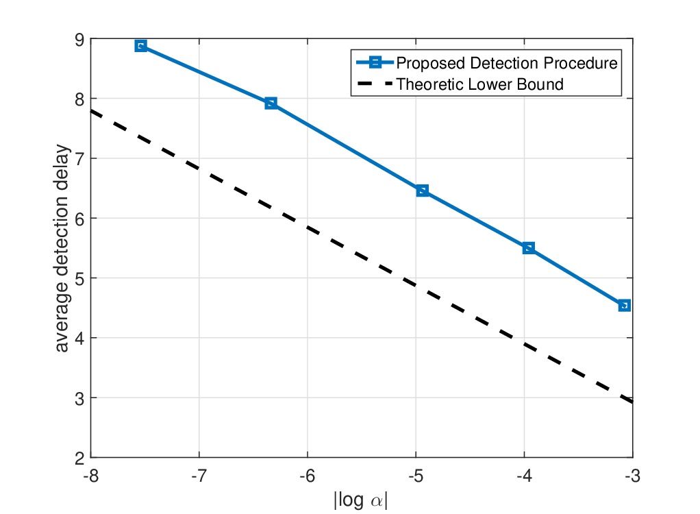
Refer to caption
Fig. 5: The performance of window based modified M-SR procedure for three mutually independent sequences

VII Conclusion

In this paper, we have considered the Bayesian QCD problem with unknown post-change parameters. In this case, we have proposed two low complexity multi-chart detection procedures, namely the M-SR procedure and the modified M-SR procedure, and have shown these two multi-chart detection procedures are asymptotically optimal when Λ\Lambda, the feasible set of the post-change parameter, is finite and asymptotically ϵ−\epsilon-optimal when Λ\Lambda is an interval. We have also considered the multi-source monitoring problem with unknown post-change parameters. In this case, we have proposed a window-based modified M-SR detection procedure and have shown its asymptotic optimality. Both the computational complexity and storage requirement of the proposed algorithm have been shown to be on the order of O⁡(mα​∑l=1LIl)O(m_{\alpha}\sum_{l=1}^{L}I_{l}).

References

  • [1] J. Geng and L. Lai, “Bayesian quickest detection with unknown post-change parameter,” in Proc. IEEE Intl. Conf. on Acoustics, Speech, and Signal Processing, (Shanghai, China), Mar. 2016.
  • [2] S. J. Kim and G. B. Giannakis, “Sequential and cooperative sensing for multichannel cognitive radios,” IEEE Trans. Signal Processing, vol. 58, pp. 4239–4253, Aug. 2010.
  • [3] Q. Zou, S. Zheng, and A. H. Sayed, “Cooperative sensing via sequential detection,” IEEE Trans. Signal Processing, vol. 58, pp. 6266–6283, Dec. 2010.
  • [4] L. Lai, Y. Fan, and H. V. Poor, “Quickest detection in cognitive radio: A sequential change detection framework,” in Proc. IEEE Global Telecommunications Conf., (New Orleans, Louisiana, USA), Nov. 2008.
  • [5] A. N. Shiryaev, “The problem of the most rapid detection of a disturbance in a stationary process,” Soviet Math. Dokl., no. 2, pp. 795–799, 1961. (translation from Dokl. Akad. Nauk SSSR vol. 138, pp. 1039-1042, 1961).
  • [6] A. N. Shiryaev, “On optimal methods in quickest detection problems,” Theory of Probability and Its Applications, vol. 8, pp. 22–46, 1963.
  • [7] G. Lorden, “Procedures for reacting to a change in distribution,” Annals of Mathematical Statistics, vol. 42, no. 6, pp. 1897–1908, 1971.
  • [8] M. Pollak, “Optimal detection of a change in distribution,” Annals of Statistics, vol. 13, pp. 206–227, Mar. 1985.
  • [9] A. G. Tartakovsky and V. V. Veeravalli, “General asymptotic Bayesian theory of quickest change detection,” Theory of Probability and Its Applications, vol. 49, no. 3, pp. 458–497, 2005.
  • [10] E. Bayraktar, S. Dayanik, and I. Karatzas, “Adaptive poisson disorder problem,” Annals of Applied Probability, vol. 16, pp. 1190–1261, 2006.
  • [11] S. Dayanik, C. Goulding, and H. V. Poor, “Bayesian sequential change diagnosis,” Mathematics of Operations Research, vol. 33, no. 2, pp. 475–496, 2008.
  • [12] S. Dayanik and C. Goulding, “Detection and identification of an unobservable change in the distribution of a Markov-modulated random sequence,” IEEE Trans. Inform. Theory, vol. 55, pp. 3323–3345, July 2009.
  • [13] G. V. Moustakides, “Optimal stopping times for detecting changes in distribution,” Annals of Statistics, vol. 14, no. 4, pp. 1379–1387, 1986.
  • [14] G. Lorden, “Open-ended tests for Koopman-Darmois families,” Annals of Statistics, vol. 1, no. 4, pp. 633–643, 1973.
  • [15] T. L. Lai, “Sequential changepoint detection in quality control and dynamical systems,” Journal of the Royal Statistical Society, vol. 57, pp. 613–658, 1995.
  • [16] M. Pollak, “Average run lengths of an optimal method of detecting a change in distribution,” Annals of Statistics, vol. 15, pp. 749–779, 1987.
  • [17] T. L. Lai, “Information bounds and quickest detection of parameter changes in stochastic systems,” IEEE Trans. Inform. Theory, vol. 44, no. 7, pp. 2917–2929, 1998.
  • [18] H. Yang, O. Hadjiliadis, and M. Ludkovski, “Detection and identification in the Wiener disorder problem with post-change drift uncertainty,” Stochastics, vol. 89, no. 3-4, pp. 654–685, 2017.
  • [19] T. Banerjee and V. V. Veeravalli, “Data-efficient minimax quickest change detection with composite post-change distribution,” IEEE Trans. Inform. Theory, vol. 61, no. 9, pp. 5172–5184, 2015.
  • [20] A. Tartakovsky, I. Nikiforov, and M. Basseville, Sequential Analysis: Hypothesis Testing and Changepoint Detection. New York: CRC Press, 2014.
  • [21] S. Dayanik, W. B. Powell, and K. Yamazaki, “Asymptotically optimal Bayesian sequential change detection and identification rules,” Annals of Operations Research, vol. 208, no. 1, pp. 337–370, 2013.
  • [22] E. Bayraktar and M. Ludkovski, “Sequential tracking of a hidden Markov chain using point process observations,” Stochastic Processes and their Applications, vol. 119, pp. 1792–1822, June 2009.
  • [23] E. Bayraktar and S. Sezer, “Online change detection for a Poisson process with a phase-type change-time prior distribution,” Sequential Analysis: Design Methods and Application, vol. 28, pp. 218–250, 2009.
  • [24] E. Bayraktar and M. Ludkovski, “Inventory management with partially observed non-stationary demand,” Annals of Operations Research, vol. 176, pp. 7–39, 2010.
  • [25] A. G. Tartakovsky and A. S. Polunchenko, “Quickest changepoint detection in distributed multisensor systems under unknown parameters,” in Proc. Intl. Conf. on Information Fusion, (Cologne, Germany), pp. 878–885, Jul. 2008.
  • [26] Y. Mei, “Efficient scalable schemes for monitoring a large number of data streams,” Biometrika, vol. 97, no. 2, pp. 419–433, 2010.
  • [27] I. V. Nikiforov, “A simple change detection scheme,” Signal Processing, vol. 81, pp. 149–172, 2001.
  • [28] T. L. Lai, “On rr-quick convergence and a conjecture of Strassen,” Annals of Probability, vol. 4, pp. 612–627, 1976.
  • [29] A. G. Tartakovsky, “Asymptotic optimality of certain multihypothesis sequential tests: non-i.i.d. case,” Statistical Inference for Stochastic Processes, vol. 1, no. 3, pp. 265–295, 1998.
  • [30] V. P. Dragalin, A. G. Tartakovsky, and V. V. Veeravalli, “Multihypothesis sequential probability ratio tests – Part I: Asymptotic optimality,” IEEE Trans. Inform. Theory, vol. 45, pp. 2448–2461, Nov. 1999.