UCLA/17/TEP/105 NORDITA-2017-071 UUITP-29/17

The Five-Loop Four-Point Integrand of ${{\cal N}=8}$ Supergravity
as a Generalized Double Copy

Zvi Bern^a, John Joseph Carrasco^b, Wei-Ming Chen^a, Henrik Johansson^c,d, Radu Roiban^e and Mao Zeng^a Affiliation:
^aMani L. Bhaumik Institute for Theoretical Physics
UCLA Department of Physics and Astronomy Los Angeles, CA 90095, USA
^bInstitute of Theoretical Physics (IPhT),
CEA-Saclay and University of Paris-Saclay
F-91191 Gif-sur-Yvette cedex, France
^cDepartment of Physics and Astronomy, Uppsala University, 75108 Uppsala, Sweden
^dNordita, Stockholm University and KTH Royal Institute of Technology, Roslagstullsbacken 23, 10691 Stockholm, Sweden
^eInstitute for Gravitation and the Cosmos, Pennsylvania State University, University Park, PA 16802, USA

Abstract

We use the recently developed generalized double-copy procedure to construct an integrand for the five-loop four-point amplitude of ${{\cal N}=8}$ supergravity. This construction starts from a naive double copy of the previously computed corresponding amplitude of ${{\cal N}=4}$ super-Yang-Mills theory. This is then systematically modified by adding contact terms generated in the context of the method of maximal unitarity cuts. For the simpler generalized cuts, whose corresponding contact terms tend to be the most complicated, we derive a set of formulas relating the contact contributions to the violations of the dual Jacobi identities in the relevant gauge-theory amplitudes. For more complex generalized unitarity cuts, which tend to have simpler contact terms associated with them, we use the method of maximal cuts more directly. The five-loop four-point integrand is a crucial ingredient towards future studies of ultraviolet properties of ${{\cal N}=8}$ supergravity at five loops and beyond. We also present a nontrivial check of the consistency of the integrand, based on modern approaches for integrating over the loop momenta in the ultraviolet region.

pacs

04.65.+e, 11.15.Bt, 11.25.Db, 12.60.Jv

I Introduction

In recent years there has been enormous progress in our ability to construct supergravity scattering amplitudes at high loop orders. This progress flows primarily from three classes of conceptual and technical advances. The first is the development of the unitarity method [1, 2], which offer a straightforward algorithmic approach to constructing and verifying multiloop integrands using only on-shell tree amplitudes. The second is the discovery of the Bern-Carrasco-Johansson (BCJ) color-kinematics duality and associated double-copy procedure [3, 4]. The third is the progress in loop integration methods, specifically integration-by-parts (IBP) reduction [5, 6, 7, 8, 9], which has been critical to extracting ultraviolet information, as in Refs. [10, 11, 12, 13, 14, 15].

In this paper we will describe in more detail the generalized double-copy procedure recently introduced in Ref. [16], which combines elements of generalized unitarity and color-kinematics duality to convert generic gauge-theory loop integrands into gravity ones. We use the method to construct the five-loop four-point integrand of ${{\cal N}=8}$ supergravity [17], which is an important stepping stone towards unraveling the ultraviolet properties of this theory. The organization of the resulting amplitude is provided by the method of maximal cuts [2]. A number of other related on-shell methods have also been developed for constructing multiloop integrands, especially for supersymmetric theories in four dimensions [18]. There are also promising methods for directly constructing integrated expressions for amplitudes, especially for ${{\cal N}=4}$ super-Yang-Mills theory in four dimensions (e.g. see Ref. [19]).

The duality between color and kinematics plays a central role in our construction. Whenever representations of gauge-theory integrands are constructed which manifest the duality between color and kinematics, corresponding gravity integrands follow directly via the double-copy procedure [4], which replaces color factors with kinematic factors. The duality applies to wide classes of gauge and gravity theories [3, 4, 20, 21, 22, 23], where, in many cases, the duality has been proven at tree level [24, 25, 26, 27, 28, 29, 30]. At loop level the duality has conjectural status, supported by case-by-case explicit calculations. The duality has been crucial in the construction of numerous gravity multiloop amplitudes [4, 11, 31, 32], where it has been used to identify new nontrivial ultraviolet cancellations in ${{\cal N}=4}$ and ${{\cal N}=5}$ supergravity [13, 15], known as ‘enhanced cancellations’. Apart from offering a simple means for obtaining loop-level scattering amplitudes in a multitude of (super)gravity theories, the duality also addresses the construction of black-hole and other classical solutions [33] including those potentially relevant to gravitational-wave observations [34], corrections to gravitational potentials [35], the relation between supergravity symmetries and gauge-theory ones [36, 20, 22], and the construction of multiloop form factors [37]. The duality has also been identified in a wider class of quantum field and string theories [38, 39, 40, 30, 41]. For recent reviews, see Ref. [42].

However, experience shows that it can sometimes be difficult to find multiloop integrands where the duality is manifest [43]. The best known example is the five-loop four-point integrand of ${{\cal N}=4}$ super-Yang-Mills theory [44], which has so far resisted all attempts to construct a BCJ representation where the duality between color and kinematics manifestly holds. This amplitude is crucial for unraveling ultraviolet cancellations that are known to exist in supergravity theories but for which no symmetry explanation has been given [15]. Because of the complexity of gravity amplitudes at high loop orders, alternative methods have offered no path forward; the only currently-known practical means for constructing the five-loop amplitude is to use a double-copy procedure that recycles the corresponding gauge-theory amplitude [44]. More generally, we would like to have a technique that converts any form of a gauge-theory integrand into the corresponding gravity ones.

A solution to this technical obstruction has been recently proposed in Ref. [16], which introduced a generalized double-copy procedure which makes use of general representations of the gauge-theory integrand. This new approach builds on the central premise of double-copy construction, but relies only on the proven existence of BCJ duality at tree level. Generic representations of gauge-theory integrands that use $f^{abc}$ color factors are double copied, giving a ‘naive double copy’. If algebraic relations obeyed by the color factors are not mirrored by the kinematic factors, however, this alone does not result in a correct gravity integrand. Violations of the kinematic algebra (dual to the color Lie algebra) must be compensated. These violations, or ‘BCJ discrepancy functions’, are the building blocks for new formulas that give corrections to the naive double copy. The correction formulas merge seamlessly with the method of maximal cuts to constructively build gravity predictions from generic gauge-theory integrands. These correction formulas also have a double-copy structure, being bilinear in the discrepancy functions of each gauge theory.

The starting point of our construction of the five-loop four-point amplitude of ${{\cal N}=8}$ supergravity is the representation of the ${{\cal N}=4}$ super-Yang-Mills amplitude given in Ref. [44], with a slight rearrangement of a few terms. The supergravity amplitude is constructed via the generalized double-copy procedure. In principle, there could have been up to 70,690 diagrammatic contributions with up to millions of terms each. Fortunately the vast majority of these diagrams either vanish or are much simpler than naive power counting suggests. Still the expressions are lengthy, and the final result is collected in a Mathematica-readable attachment [45].

To confirm our integrand, we carried out a number of nontrivial checks. Besides the generalized cuts used in the construction, we also check consistency of large numbers of additional generalized unitary cuts. We numerically confirmed in all cases where the new formulas are used that a less efficient evaluation of the gravity unitarity cuts, based on Kawai-Lewellen-Tye tree-level relations, gives identical results. We also present nontrivial checks based on integrating the expressions in spacetime dimension $D=22/5$ , where we expect it to be finite, yet individual terms in our expression diverge. To carry out these checks we develop techniques based on modern developments in integration [7, 9, 46, 47]. We carry out the check using both unitarity-compatible IBP methods as well as a new method of direct integration described in Appendix B.

We leave for the future the much more interesting—and much more difficult—case of integrating in dimension $D=24/5$ , where symmetry arguments suggest that a divergence could be present [48, 49]. The discovery of enhanced ultraviolet cancellations in closely-related supergravity theories [13, 15] suggests, however, that the five-loop amplitude might nonetheless be finite in $D=24/5$ . A direct integration of our integrand would settle the issue.

This paper is organized as follows. First, in Section II, we present a brief review of the method of maximal cuts and the double-copy construction. Then, in Section III, we give an overview of the derivation of the new formulas for obtaining correction to the naive double copy in terms of BCJ discrepancy functions. In Section IV, we derive the explicit formulas giving the contact term corrections, involving two four-point contact interactions or one five-point interaction. This is generalized to infinite classes of contact interactions in Section V. The results for the five-loop four-point integrand of ${{\cal N}=8}$ supergravity are described in Section VI. In Section VII, we series expand the integrand in large loop momenta and perform nontrivial integration checks demonstrating its consistency. Our conclusions and outlook are given in Section VIII. Two appendices are included; the first gives correction formulas useful for contact diagrams with four canceled propagators and the second describes a unitarity-compatible direct integration of vacuum diagrams generated by series expanding the integrand.

II Review

In the mid 1980s string-theory investigations by Kawai, Lewellen and Tye (KLT) [50] exposed remarkable relations between closed- and open-string tree-level scattering amplitudes. Since string-theory tree-level amplitudes have smooth low-energy limits to gauge and gravity field theory amplitudes, this had a number of implications for field-theory predictions [51, 52]. With the advent of unitarity methods [1], these tree-level insights have direct impact on our ability to calculate at loops as well as on our basic understanding of the structure of gravity loop amplitudes [53, 52]. With the understanding of the duality between color and kinematics, much simpler and powerful means for generating gravity loop amplitudes from gauge theory became available [3, 4]. We begin with a lightning review of double-copy structure of gravity amplitudes, before discussing application of the method of maximal cuts relevant for our construction [16].

II.1 Tree-level gravity amplitudes from gauge theory

II.1.1 BCJ duality and double-copy amplitudes

All tree-level amplitudes in any $D$ -dimensional gauge theory coupled to fields in the adjoint representation, may be written as

\mathcal{A}^{{\rm tree}}_{m}=g^{m-2}\sum_{j\in\Gamma_{3,m}}\frac{c_{j}n_{j}}{D_{j}}\,,

(1)

where sum is over the set of $(2m-5)!!$ distinct, $m$ -point graphs with only cubic (trivalent) vertices, which we denote by $\Gamma_{3,m}$ . These graphs are sufficient because the contribution of any diagram with quartic or higher vertices can be assigned to a graph with only cubic vertices by multiplying and dividing by appropriate propagators. The nontrivial kinematic information is contained in the numerators $n_{j}$ and generically depends on momenta, polarizations, and spinors. The color factor $c_{j}$ is obtained by dressing every vertex in graph $j$ with the relevant gauge-group structure constant, $\tilde{f}^{abc}=i\sqrt{2}f^{abc}=\mathrm{Tr}([T^{a},T^{b}]T^{c})$ , where the Hermitian generators of the gauge group are normalized via $\mathrm{Tr}(T^{a}T^{b})=\delta^{ab}.$ The denominator $1/D_{j}$ contains the Feynman propagators of the graph $j$

\frac{1}{D_{j}}\equiv\frac{1}{\prod_{i_{j}}d_{i_{j}}}\,,

(2)

where $i_{j}$ runs over the propagators for diagram $j$ , each of which we denote by $1/d_{i_{j}}$ . The gauge-theory coupling constant is $g$ . If an on-shell superspace is used the numerators will also depend on anticommuting parameters.

Refer to caption — Figure 1: The three diagrams with only cubic vertices contributing to a four-point tree amplitude.

In a BCJ representation, kinematic numerators obey the same generic algebraic relations as the color factors [3, 4, 11, 42]. For theories with only fields in the adjoint representation there are two properties. The first property is antisymmetry under graph vertex flips:

c_{\overline{i}}=-c_{i}\ \Rightarrow\ n_{\overline{i}}=-n_{i}\,,

(3)

where the graph $\overline{i}$ has same graph connectivity as graph $i$ , except an odd number of vertices have been cyclically reversed. The second property is the requirement that all Jacobi identities are satisfied,

c_{i}+c_{j}+c_{k}=0\ \Rightarrow\ n_{i}^{\rm BCJ}+n_{j}^{\rm BCJ}+n_{k}^{\rm BCJ}=0\,,

(4)

where $i$ , $j$ , and $k$ refer to three graphs which are identical except for one internal edge. For example at four points the color factors of the three diagrams listed in Fig. 1 obey the Jacobi identity.

Once corresponding gauge-theory loop integrands have been arranged into a form where the duality is manifest [3, 4], it is then easy to obtain gravity loop integrands: one simply replaces the color factors of a gauge-theory integrand with the kinematic numerators of another gauge-theory integrand,

c_{i}\ \rightarrow\ \tilde{n}_{i}\,.

(5)

This immediately gives the double-copy form of a gravity tree amplitude,

\mathcal{M}^{{\rm tree}}_{m}=i\left(\frac{\kappa}{2}\right)^{m-2}\sum_{j\in\Gamma_{3,m}}\frac{\tilde{n}_{j}n_{j}}{D_{j}}\,,

(6)

where $\kappa$ is the gravitational coupling and $\tilde{n}_{j}$ and $n_{j}$ are the kinematic numerator factors of the two gauge theories. Only one of the two sets of numerators needs to manifestly satisfy the duality (4) [4, 24] in order for the double-copy form (6) to be valid.

II.1.2 Ordered partial amplitudes

The color factors, $c_{i}$ in Eq. (1), can be expressed in a color-trace basis. Collecting associated kinematic factors yields,

\mathcal{A}^{{\rm tree}}_{m}=g^{m-2}\sum_{\rho\in{\cal S}_{m-1}}\mathrm{Tr}\left(T^{\rho_{1}}T^{\rho_{2}}\ldots T^{\rho_{m}}\right)A^{{\rm tree}}_{m}(\rho_{1},\rho_{2},\ldots,\rho_{m})\,.

(7)

where the sum runs over the set ${\cal S}_{m-1}$ of non-cyclic permutations. The $A^{{\rm tree}}_{m}(\rho)$ are called color-ordered partial amplitudes., The terminology ordered refers to the fact that all graphs contributing to any given $A^{{\rm tree}}_{m}(\rho)$ have the same ordering or external legs as the cyclic ordering of the color trace ${\rm Tr}(\rho)$ . We can write the color-ordered amplitudes in terms of graphs via

A^{{\rm tree}}_{m}(1,\rho_{2},\ldots,\rho_{m})=\sum_{i\in\Gamma_{\rho}}\frac{n_{i}}{D_{i}}\,,

(8)

where $\Gamma_{\rho}$ refers to the graphs with cubic vertices where the legs are ordered following the color ordering.

The partial-ordered amplitudes in Eq. (7) are not independent and can be reduced to a sum over $(m-2)!$ partial amplitudes using color-Jacobi identities [54]

\mathcal{A}^{{\rm tree}}_{m}=g^{m-2}\sum_{\rho\in{\cal S}_{m-2}}c(1|\rho_{2},\ldots,\rho_{m-1}|m)A^{{\rm tree}}_{m}(1,\rho_{2},\ldots,\rho_{m-1},m)\,,

(9)

where $c(1|\rho_{2},\ldots,\rho_{m-1}|m)$ is the color factor of the half-ladder diagram in Fig. 2. Replacing $c(1|\rho|m)$ by a color-dual kinematic numerator of the same half-ladder graph $n^{{\rm BCJ}}(1|\rho|m)$ , and taking into account the appropriate ratio of coupling constants indeed yields another representation of gravity tree amplitudes [24]:

\mathcal{M}^{{\rm tree}}_{m}=i\left(\frac{\kappa}{2}\right)^{m-2}\sum_{\rho\in{\cal S}_{m-2}}\tilde{n}^{{\rm BCJ}}(1|\rho_{2},\ldots,\rho_{m-1}|m)A^{{\rm tree}}_{m}(1,\rho_{2},\ldots,\rho_{m-1},m)\,.

(10)

II.1.3 KLT relations

The KLT relations [50] give direct relations between gravity and gauge-theory tree amplitude. The KLT formulas can be obtained from BCJ duality, by using Jacobi identities to express all kinematic numerators in Eq. (8) in terms of a basis of $(m-2)!$ numerators, called master numerators. One can then (pseudo-)invert the relationship between a minimal basis of $(m-3)!$ independent ordered amplitudes to solve for the master numerators in terms of partial amplitudes. Indeed, the availability of a color-dual form for kinematic numerators is responsible for the reduction to a basis of $(m-3)!$ [3]. As the propagator matrix is singular, such pseudo-inversions are not unique, so there are many possibilities.

The first such formula valid for an arbitrary number of legs was given in Appendix A of Ref. [52]. It remains as a particularly sparse and efficient form, so we use it for directly constructing gravity unitarity cuts. The tree-level relation is

$\displaystyle{\cal M}^{\rm tree}_{m}(1,2,\ldots,m)$	$\displaystyle=$	$\displaystyle i(-1)^{m+1}\Bigl({\kappa\over 2}\Bigr)^{m-2}\Bigl[A^{\rm tree}_{m}(1,2,\ldots,m)\displaystyle\sum_{\rm perms}f(i_{1},\ldots,i_{j})\overline{f}(l_{1},\ldots,l_{j^{\prime}})$	(11)
		$\displaystyle\hskip 85.35826pt\hbox{}\times\tilde{A}^{\rm tree}_{m}(i_{1},\ldots,i_{j},1,m-1,l_{1},\ldots,l_{j^{\prime}},m)\Bigr]$
		$\displaystyle\hbox{}\hskip 28.45274pt+{\rm Perm}(2,\ldots,m-2)\,,$

where $A_{m}$ and $\tilde{A}_{m}$ are two $m$ -point gauge-theory amplitudes from each of the two copies. The sum is over all permutations $\{i_{1},\ldots,i_{j}\}\in{\rm Perm}\{2,\ldots,\lfloor m/2\rfloor\}$ and $\{l_{1},\ldots,l_{j^{\prime}}\}\in{\rm Perm}\{\lfloor m/2\rfloor+1,\ldots,m-2\}$ with $j=\lfloor m/2\rfloor-1$ and $j^{\prime}=\lfloor m/2\rfloor-2$ , which gives a total of $(\lfloor m/2\rfloor-1)!\times(\lfloor m/2\rfloor-2)!$ terms inside the square brackets. The notation “ $+\,{\rm Perm}(2,\ldots,m-2)$ ” signifies a sum over the expression for all permutations of legs $2,\ldots,m-2$ . The functions $f$ and $\overline{f}$ are given by,

	$\displaystyle f(i_{1},\ldots,i_{j})$	$\displaystyle=$	$\displaystyle s_{1,i_{j}}\prod_{m=1}^{j-1}\left(s_{1,i_{m}}+\sum_{k=m+1}^{j}g(i_{m},i_{k})\right),$
	$\displaystyle\overline{f}(l_{1},\ldots,l_{j^{\prime}})$	$\displaystyle=$	$\displaystyle s_{l_{1},m-1}\prod_{m=2}^{j^{\prime}}\left(s_{l_{m},m-1}+\sum_{k=1}^{m-1}g(l_{k},l_{m})\right),$		(12)

and

g(i,j)=\left\{\begin{array}[]{ll}s_{i,j}&\mbox{if $i>j$,}\\ 0&\mbox{otherwise.}\end{array}\right.

(13)

By applying BCJ amplitude relations [3], many different versions of KLT relations can be constructed [26], including a tidy recursive definition [40]. The general form of the KLT relations in terms of a basis of gauge-theory amplitudes may be written as,

	$\displaystyle\mathcal{M}^{{\rm tree}}_{m}=$	$\displaystyle\hbox{}i\left(\frac{\kappa}{2}\right)^{m-2}\sum_{\tau,\rho\in{\cal S}_{m-3}}K(\tau\|\rho)\tilde{A}^{{\rm tree}}_{m}\left(1,\rho_{2},\ldots,\rho_{m-2},m,(m-1)\right)$
		$\displaystyle\hskip 56.9055pt\times A^{{\rm tree}}_{m}\left(1,\tau_{2},\ldots,\tau_{m-2},(m-1),m\right)\,,$		(14)

where the sum runs over $(m-3)!$ permutations of external legs. The KLT matrix $K(\tau|\rho)$ , indexed by the elements of the two permutation orderings of the relevant partial amplitudes, also called a momentum kernel, depends only on momentum invariants arising from inverse propagators.

Not only do the various versions of KLT kernels follow from color-kinematics duality, but a comparison of Eq. (10) and Eq. (14) gives a useful non-local representation of color-dual BCJ numerators from color-ordered partial amplitude [25, 26]. This gives a set of explicit nonlocal BCJ numerators,

	$\displaystyle n^{\rm BCJ}(1\|\tau_{2},\ldots,$	$\displaystyle\tau_{m-2},\tau_{m-1}\|m)$
		$\displaystyle=\left\{\begin{array}[]{lc}\displaystyle\sum_{\rho\in{\cal S}_{m-3}}K(\tau\|\rho)A^{{\rm tree}}_{m}(1,\rho_{2},\ldots\rho_{m-2},m,(m-1))\,,&\hskip 17.07182pt\hbox{if }\tau_{m-1}=m-1\,,\\ 0\,,&\hskip 17.07182pt\hbox{if }\tau_{m-1}\not=m-1\,.\end{array}\right.$

In this formula the permutations of $(m-2)$ legs of the half ladder is effectively reduced to a permutation sum over $(m-3)$ legs, because some of the numerators vanish. Numerators of diagrams which are not of the half-ladder form in Fig. 2 follow from the dual Jacobi relations (4). Equation (II.1.3) is useful below to derive KLT forms of unitarity cuts from BCJ forms.

II.2 Method of maximal cuts

We now review the method of maximal cuts [2] applied to building a double-copy gravity integrand. The method of maximal cuts is a refinement of the generalized unitarity method [1]. We organize the maximal cut method in a constructive way, assigning new contributions to new contact diagrams as one proceeds. (For recent examples, see Refs. [55, 16].) In subsequent sections we will describe how to make this procedure efficient for gravity theories at high loop orders, by recycling gauge-theory results.

The method of maximal cuts [2] constructs multiloop integrands from generalized unitarity cuts. These cuts cluster in levels according to the number of internal propagators $k$ allowed to remain off shell,

\displaystyle{\cal C}^{{\rm N}^{k}{\rm MC}}

\displaystyle=\sum_{\rm states}{\cal A}_{m(1)}^{\rm tree}\cdots{\cal A}_{m(p)}^{\rm tree}\,,

\displaystyle k\equiv\sum^{p}_{i=1}m(i)-3p\,,

(17)

where the ${\cal A}_{m(i)}^{\rm tree}$ are tree-level $m(i)$ -multiplicity amplitudes corresponding to the blobs, illustrated in Figs. 3 and 4. This is valid for either gauge or gravity amplitudes. In the gauge-theory case, the state sum also includes sums over internal color. As illustrated in the first diagram in Fig. 3, at the maximal cut (MC) level the maximum number of propagators are replaced by on shell conditions and all tree amplitudes appearing in Eq. (17) are three-point amplitudes. At the next-to-maximal-cut (NMC) level a single propagator is placed off shell and so forth. We will categorize different cuts at level $k$ by the contained tree amplitudes with four or more legs: an $m_{1}\times m_{2}\times\cdots\times m_{q}$ cut contains one tree amplitude with $m_{1}$ legs, one with $m_{2}$ legs and so forth.

In the method of maximal cuts, the integrands for $L$ -loop amplitudes are obtained by first establishing an integrand whose maximal cuts are correct, then adding to it terms so that NMCs are all correct and systematically proceeding through the next^k maximal cuts (N^kMCs), until no further contributions can be found. Where this happens is dictated by the power counting of the theory and by choices made at each level. For example, if a minimal power counting is assigned to each contribution, for ${{\cal N}=4}$ super-Yang–Mills four-point amplitudes, cuts through NMCs, N²MCs and N³MCs are sufficient at three [4], four [11] and five loops [44], respectively.

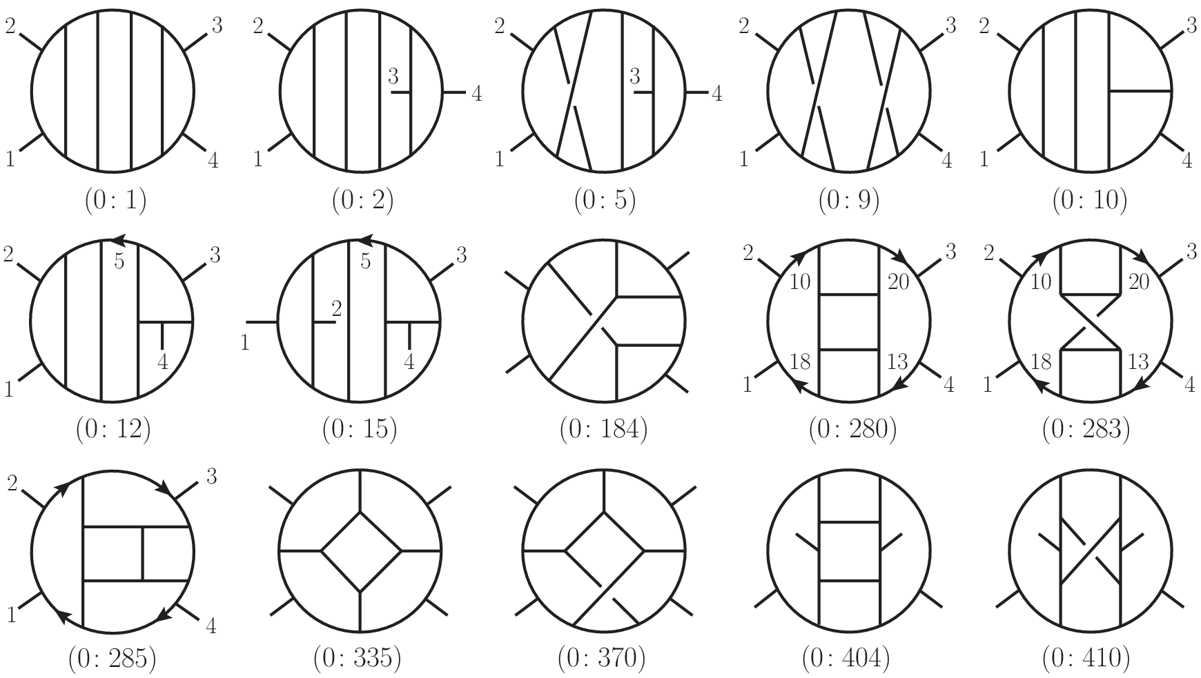
Most previous calculations (see e.g., Refs. [10, 11, 12, 13, 14, 15, 43, 37]) found it convenient to organize the results in terms of purely cubic diagrams, assigning all higher-order missing N^kMC data to the parent graphs with only cubic vertices, such as the five-loop ones illustrated in Fig. 5. Representations with only cubic diagrams have useful advantages: they are useful for establishing minimal power counting in each diagram, and the number of graphs used to describe the result proliferate minimally with loop order and multiplicity¹¹ 1 Though still factorially.. A disadvantage is that Ansätze are required to impose the higher-order data on each graph while respecting power counting, symmetry, and the multiple unitarity cuts to which a given diagram contributes. As the loop order increases, it becomes cumbersome to solve the requisite system of equations that imposes these constraints.

II.3 Naive double copy and contact diagram corrections

For our purposes of constructing the five-loop four-point integrand it is better to directly assign new cut data to contact graphs in one-to-one correspondence to the N^kMC, as in the original method of maximal cuts construction [2], avoiding Ansätze for the amplitudes. We now describe this organizational principle in the context of obtaining high-loop-order gravity integrands.

The starting point in our gravity construction is a gauge-theory integrand, whose terms are assigned to only graphs with cubic vertices. The actual gauge-theory amplitude would be given:

{\cal A}_{m}^{L\text{-loop}}=i^{L}g^{2L+m-2}\sum_{{\cal S}_{m}}\sum_{i\in\Gamma_{3,m,L}}\int\prod_{j}^{L}\frac{d^{D}l_{j}}{(2\pi)^{D}}\frac{1}{S_{i}}\frac{c_{i}n_{i}}{D_{i}}\,,

(18)

where the first sum runs over the set ${\cal S}_{m}$ of external leg permutations. The second sum runs over the set of diagrams $\Gamma_{3,m,L}$ with only three vertices, $m$ external points and $L$ loops. The symmetry factors $S_{i}$ for each diagram $i$ remove overcounts, including those arising from internal automorphism symmetries with external legs fixed. As in Section II.1, the color factors $c_{i}$ of all graphs are obtained by dressing every three-vertex in the graph with a factor of $\tilde{f}^{abc}=\,{\rm Tr}([T^{a},T^{b}]T^{c})$ , where the gauge group generators $T^{a}$ are normalized via $\,{\rm Tr}(T^{a}T^{b})=\delta^{ab}$ . As before, the gauge coupling is $g$ . The kinematic numerators, $n_{i}$ , are functions of momenta, spinors, and polarization vectors. As usual, the $1/D_{i}$ signify the product of Feynman propagators of diagram $i$ .

Our construction starts with a naive double copy, which we call the ‘level 0’ or ’top-level’ contribution,

{\cal M}_{m}^{L\text{-loop}}=i^{L+1}\left(\frac{\kappa}{2}\right)^{2L+m-2}\sum_{{\cal S}_{m}}\sum_{i\in\Gamma_{3,m,L}}\int\prod_{j}^{L}\frac{d^{D}l_{j}}{(2\pi)^{D}}\frac{1}{S^{(0)}_{i}}\frac{N^{(0)}_{i}}{D_{i}}\,,

(19)

where the level 0 numerators are just double copies of gauge-theory numerators,

N^{(0)}_{i}=n_{i}\tilde{n}_{i}\,.

(20)

If the gauge-theory $n_{i}$ satisfy the BCJ relations (4), then we have the complete gravity integrand and we would be done [4]. However, when the gauge-theory integrand (18) does not manifest BCJ duality, our naive double copy requires corrections to become a gravity integrand, as we can systematically determine by evaluating generalized cuts.

First we should note that all maximal cuts (MCs) and all next to maximal cuts (NMCs) will be automatically satisfied by our naive double copy. The reason is that on-shell ( $D$ -dimensional) supergravity three-point amplitude is just the square of the ${{\cal N}=4}$ super-Yang-Mills ones,

{\cal M}_{3}^{{{\cal N}=8}\,{\rm tree}}(1,2,3)=i\frac{\kappa}{2}\Bigl[A_{3}^{{{\cal N}=4}\,{\rm tree}}(1,2,3)\Bigr]^{2}\,,

(21)

for all states of the theory. All NMCs are also automatically satisfied because color-kinematics duality automatically holds for the four-point tree amplitudes [3]. Examples of MCs and NMCs are given in Fig. 3.

Starting with the N²MCs, the cuts of the naive-double copy no longer generically match the actual cuts of the double-copy gravity theory. Because the naive double copy automatically gives the correct MCs and NMCs, the correction terms are necessarily contact terms involving two or more collapsed propagators. The cut conditions are then solved starting from the N²MCs and proceeding towards the higher $k$ N^kMCs. At each new cut level the only new information is captured by contact terms as illustrated in Fig. 6. Fig. 7 displays the contact diagrams representing the new information contained in the generalized cuts of Fig. 4.

The contact terms are defined as differences between a cut of the complete gravity amplitude and the cut of our partially-constructed gravity amplitude. The gravity generalized cuts can in principle all be obtained by plugging gravity tree amplitudes obtained from the KLT tree relations into Eq. (11) into the generalize cut (17), although this is rather inefficient. We also define an incomplete integrand ${\cal I}^{k}$ given by starting from the naive double copy and including all contact terms through level $(k-1)$ . At any level $k$ we define the incomplete integrand to be the sum over all diagrams from level zero to level $(k-1)$ ,

{\cal I}^{(k)}=\sum_{\ell=0}^{k-1}\sum_{{\cal S}_{m}}\sum_{i_{\ell}}\frac{1}{S^{(\ell)}_{i_{\ell}}}\frac{N^{(\ell)}_{i_{\ell}}}{D^{(\ell)}_{i_{\ell}}}\,,

(22)

where the sum over $\ell$ is over the contact term levels up to level $k-1$ and the sum over $i_{\ell}$ is over diagrams at level $\ell$ . The $N^{(\ell)}_{i}$ , $S^{(\ell)}_{i}$ and $D^{(\ell)}_{i}$ are respectively the numerators, symmetry factors and kinematic denominators for diagram $i$ at level $k$ . As usual the sum over ${{\cal S}_{m}}$ represents the sum over the $m!$ permutations of external legs. The kinematic denominators are composed of products of Feynman propagators for each diagram.

Starting from the gravity cut, ${\cal C}^{{\rm N}^{k}{\rm MC}}$ , and subtracting from it the cut of the incomplete integrand (22), gives us the missing piece in the cut,

{\cal K}^{{\rm N}^{k}{\rm MC}}={\cal C}^{{\rm N}^{k}{\rm MC}}-{\cal I}^{k}\Bigr|_{{{\rm N}^{k}{\rm MC}}}\,,

(23)

where a N^kMC is taken. This difference can be assigned to a contact diagram because all the nonlocal contributions are accounted for at earlier levels. In this way for each cut for $k\geq 2$ there is a contact term diagram, as illustrated in Fig. 6. See also Fig. 7 for examples of contact diagrams that are in one-to-one correspondence to the generalized unitarity cuts in Fig. 4.

We promote these contact terms to off-shell expressions simply by removing all on-shell constraints,

{\cal K}^{{\rm N}^{k}{\rm MC}}\rightarrow{\cal K}^{{\rm N}^{k}{\rm MC}}\Bigr|_{\rm off\hbox{-}shell}\,.

(24)

This then defines a level- $k$ contact term assigned to a given graph, as illustrated in Fig. 6. We take the final contact diagram to be one where no cut conditions are imposed. Each non-vanishing contact graph generated this way is then incorporated into the partially constructed integrand. The generated contact diagram is not unique because one can add or subtract terms that vanish prior to releasing the cut conditions. An important constraint is that the constructed contact terms should always respect diagram symmetry, even after on-shell constraints are removed. A simple way to impose the symmetry on an arbitrary off-shell continuation is to explicitly average over all diagram symmetries. Different choices of off-shell continuations can alter higher-level contact terms. An important feature of this construction is that each contact term depends only on choices made at previous lower- $k$ levels.

The construction proceeds level by level in the cuts until no further contact terms are found. Where this happens is dictated by the power counting of the gravity theory.²² 2 For the five-loop four-point amplitude of ${{\cal N}=8}$ supergravity no new contact terms are found beyond level $k=6$ .

In general, Eq. (23) can be quite complicated to simplify, especially when the gravity cut is obtained from the KLT version of generalized cuts. It however is an efficient means to generate expressions for numerical evaluation. Far more efficient ways to analytically generate these contributions will be described in Sections III-V.

The final amplitude is obtained at the end of this process, when we reach a level $k_{\rm max}$ in the incomplete integrand (22) beyond which there are no further nonvanishing contributions. After assembling the naive double copy and contact diagrams the resulting gravity amplitude is obtained by summing over all nonvanishing levels and integrating,

{\cal M}_{m}^{L\text{-loop}}=i^{L+1}\left(\frac{\kappa}{2}\right)^{2L+m-2}\sum_{\ell}^{k_{\rm max}}\sum_{{\cal S}_{m}}\sum_{i}\int\prod_{j}^{L}\frac{d^{D}l_{j}}{(2\pi)^{D}}\frac{1}{S^{(\ell)}_{i}}\frac{N^{(\ell)}_{i}}{D^{(\ell)}_{i}}\,,

(25)

where $k_{\rm max}$ is the highest level containing nonvanishing diagrams.

II.4 Double copy and gravity unitarity cuts

In order to use Eq. (23) to obtain the missing contact diagram, we need efficient means to obtain the gravity cuts. In this subsection we explain how gauge-theory generalized cuts can be converted directly to gravity cuts, without having to go back to gravity tree amplitudes via the KLT relations (11). Once these steps have been carried out in the corresponding gauge-theory amplitudes we simply recycle them into gravity. This bypasses the nontrivial steps of having to perform state sums [56] ensuring that results are valid in $D$ -dimensions [57].

Consider a generalized unitarity cut in Eq. (17) and Fig. 4 for gauge theory. We can express each tree amplitude in terms of diagrams with only cubic vertices as in Eq. (1),

\displaystyle{\cal C}_{\rm YM}\equiv\sum_{\text{states}}\prod^{p}_{j=1}{\cal A}^{{\rm tree}}_{m(j)}

\displaystyle={\sum_{\text{states}}}\prod^{p}_{j=1}\sum_{g(j)\in\Gamma_{3,m(j)}}\,\frac{c_{g(j)}\,{n}_{g(j)}}{D_{g(j)}}\,,

(26)

where $j$ specifies the tree amplitude, $g(j)$ represents a graph of the $j$ th tree amplitude from the set of graphs $\Gamma_{3,m(j)}$ , including the trivial three-vertex for the three-point amplitude. For simplicity we have suppressed the coupling constants here and in all subsequent formulas for generalized cuts. The denominators $1/D_{g(j)}$ are composed of the Feynman propagators of the graph $g(j)$ .

By applying the color decomposition in Eq. (9) to each tree amplitude we obtain a color-decomposed form of the unitarity cut,

\displaystyle{\cal C}_{\rm YM}

\displaystyle={\sum_{\text{states}}}\,\prod^{p}_{j=1}\,\sum_{\rho^{(j)}\in{\cal S}_{m(j)-2}}c(\rho^{(j)})A_{m(j)}^{\rm tree}(\rho^{(j)})\,,

(27)

where $\rho^{(j)}$ refers to the arguments in Eq. (9), but for the $j$ th tree. The permutation ${\cal S}_{m(j)-2}$ act on $(m(j)-2)$ of the legs of the $j$ th tree amplitude. For three-point trees the permutation sum is trivial. As before, the internal color indices are included in the state sum.

Now consider generalized gravity cuts. A crucial property is that the states of double-copy theories factorize into the outer product of states of their constituent single-copy theories. In particular, for ${{\cal N}=8}$ supergravity in four dimensions, every gravity state is indexed by ‘left’ and ‘right’ ${{\cal N}=4}$ super-Yang–Mills states:

({{\cal N}=8}{\text{ SG state}})=({{\cal N}=4}{\text{ sYM state}})_{\rm L}\otimes({{\cal N}=4}{\text{ sYM state}})_{\rm R}\,.

(28)

In fact, the state sum over the entire supergravity multiplet is a double-sum over the entire super-Yang-Mills multiplet,

\sum_{{{{\cal N}=8}\ {\text{SG}}\atop\text{states}}}=\sum_{{{{\cal N}=4}\ {\text{sYM}}\atop{\text{L-states}}}}\times\sum_{{{{\cal N}=4}\ {\text{sYM}}\atop{\text{R-states}}}}\,.

(29)

This holds in $D\leq 10$ dimensions where ${{\cal N}=4}$ super-Yang–Mills theory is defined as a dimensional reduction of the $D=10$ , ${{\cal N}=1}$ theory.

Each gravity tree amplitude in the cut, such as those in Fig. 4, can be arranged into a BCJ double-copy form

\displaystyle{\cal C}_{{\rm GR}}\equiv\sum_{\text{states}}\prod^{p}_{j=1}M^{{\rm tree}}_{m(j)}=i^{p}\sum_{\text{states}_{\text{L}}}\,\sum_{\text{states}_{\text{R}}}\,\prod^{p}_{j=1}\sum_{g(j)\in\Gamma_{3,m(j)}}\;\frac{n^{\text{{\rm BCJ}}}_{g(j)}\,\tilde{n}^{\text{{\rm BCJ}}}_{g(j)}}{D_{g(j)}}\,,

(30)

where we have suppressed the gravitational coupling and $n^{\text{{\rm BCJ}}}$ and $\tilde{n}^{\text{{\rm BCJ}}}$ are kinematic numerators of the left and right gauge theories. For each tree amplitude one can always find BCJ forms for the numerators. For example, the explicit BCJ numerators in Eq. (II.1.3) for each tree amplitude immediately give the gravity amplitude starting from a gauge-theory amplitude.

We can then rearrange the cut into a KLT form, using the tree-level results from the previous subsection. Given the that BCJ form of the numerators have exactly the same algebraic properties as color factors, we write the cut in precisely the same form as the color decomposed gauge-theory cut (II.1.3)

\displaystyle{\cal C}_{{\rm GR}}

\displaystyle=i^{p}{\sum_{\text{states}}}\,\prod^{p}_{j=1}\,\sum_{\rho^{(j)}\in{\cal S}_{m(j)-2}}{\tilde{n}}^{\rm BCJ}(\rho^{(j)})A_{m(j)}^{\rm tree}(\rho^{(j)})\,,

(31)

where the numerator is that of the half-ladder diagram specified in Fig. 2. In this formula the numerators $n^{\rm BCJ}(\rho^{(j)})$ correspond to the half-ladder diagrams with an ordering of legs specified by the permutation $\rho^{(j)}$ . Here the tree subscripts $m(j)$ encode the multiplicity of the $j$ -th tree, and $m$ and $L$ are the overall multiplicity and loop order of the amplitude. Plugging in the specific BCJ numerators in Eq. (II.1.3) reduces each permutation sum from acting on $(m(j)-2)$ legs to $(m(j)-3)$ legs, given the numerator vanishings in Eq. (II.1.3).

Substituting in the explicit expression for BCJ numerators in Eq. (II.1.3) immediately gives the KLT form of the gravity generalized cut,

	$\displaystyle{\cal C}_{{\rm GR}}$	$\displaystyle=i^{p}\sum_{\text{states}}\prod^{p}_{j=1}\,\sum_{\rho^{(j)},\tau^{(j)}\in{\cal S}_{m(j)-3}}\,K(\rho^{(j)}\|\tau^{(j)})\,A^{{\rm tree}}_{m(j)}(\rho^{(j)})\,\tilde{A}^{{\rm tree}}_{m(j)}(\tau^{(j)})$
		$\displaystyle=i^{p}{\sum_{\vec{\rho},\vec{\tau}}}K(\vec{\rho}\,\|\vec{\tau})\Biggl(\sum_{\text{states}_{\text{L}}}A^{{\rm tree}}_{m(1)}(\rho^{(1)})\cdots A^{{\rm tree}}_{m(p)}(\rho^{(p)})\Biggr)\Biggl(\sum_{\text{states}_{\text{R}}}\tilde{A}^{{\rm tree}}_{m(1)}(\tau^{(1)})\cdots\tilde{A}^{{\rm tree}}_{m(p)}(\tau^{(p)})\Biggr)\,,$		(32)

where we have suppressed overall factors of the $(\kappa/2)$ gravitational coupling and

K(\vec{\rho}\,|\vec{\tau})\equiv K(\rho^{(1)}|\tau^{(1)})\cdots K(\rho^{(p)}|\tau^{(p)})\,,

(33)

and we used the factorization of the state sums as in Eq. (28). For each gauge-theory tree amplitude, the permutation sum follows that in Eq. (14). For the three- and four-point cases the permutation sum is a single term.

Equation (32) allows us construct gravity generalized unitarity cuts from corresponding gauge-theory tree amplitudes. However, it is much more efficient to apply Eq. (32) directly to cuts of previously constructed gauge-theory loop amplitudes, rather than using tree amplitudes. That is, we take Eq. (32) as a recipe for assembling color-ordered gauge-theory cuts into gravity cuts. In this way the states sums, and other simplifications are automatically inherited from the gauge-theory loop integrands. Another enormous technical advantage is that we need the cuts and the constructed loop integrand to be valid in $D$ dimensions, not just in four dimensions. In particular, explicit checks confirm the validity of the five-loop four-point amplitude of ${{\cal N}=4}$ super-Yang–Mills [44] for $D\leq 6$ [57]. This is then automatically imported into the corresponding ${{\cal N}=8}$ supergravity amplitude. It is course crucial to guarantee the validity of the expressions outside of $D=4$ dimensions, given we are interested primarily in its ultraviolet behavior in higher dimensions.

Unfortunately, even after applying Eq. (32) to convert cuts of gauge-theory loop amplitudes, the analytic expressions inherited from the KLT construction are rather complicated. This makes it difficult to analytically simplify the contact terms in Eq. (23) at high loop orders. However, it does provide a rather efficient means for numerically evaluating any cut, by first numerically evaluating the gauge-theory unitarity cuts and then carrying out the matrix multiplication in Eq. (32) numerically. This will prove very useful in Section VI, where the five-loop four-point amplitude on ${{\cal N}=8}$ supergravity is constructed. While the numerical analysis is quite helpful, especially for confirming the correctness of expressions, the required Ansätse are impractical. Much more efficient means for analytically constructing gravity contact terms are given in the next sections.

III Contact terms from BCJ duality

In the previous section we reviewed a constructive method for building up a supergravity amplitude starting from a naive double copy of a corresponding gauge-theory amplitude. However, it is still nontrivial to extract the contact terms at high loop orders, given the analytic complexity of generalized cuts obtained as obtained from Eq. (32). To deal with this, Ref. [16] outlined a method for obtaining correction terms to the naive double copy directly from corresponding gauge-theory expressions, without having to construct gravity unitarity cuts. This enormously simplifies the task. Here we elaborate on the details of this method.

III.1 Overview of gravity cuts from BCJ discrepancy functions

As noted in the previous section, at high loop orders it can be difficult to find representations of the amplitudes that manifest BCJ duality. Instead, we start from the “naive double copy” in Eq. (19), obtained by replacing the color factors with numerators that do not satisfy the duality, and correct it until it reproduces all the generalized cuts of the gravity amplitude. The properties of three and four-point gauge-theory amplitudes guarantee that the naive double copy has the correct maximal and next-to-maximal cuts. The method of maximal cuts provides a means to systematically construct the contact terms corresponding to the N^kMC with $k\geq 2$ .

The building blocks for the corrections terms are BCJ discrepancy functions, which are defined in terms of the violation of BCJ duality by a given representation of the gauge-theory amplitude,

J=n_{i}+n_{j}+n_{k}\,,

(34)

where graphs $i$ , $j$ , and $k$ are a Jacobi triplet of graphs, as in Eq. (4). As already noted in Ref. [16], we find that the corrections are quadratic in the discrepancy functions

{\cal E}_{\rm GR}\sim\sum_{a,b}g_{ab}J_{a}{\tilde{J}}_{b}\,,

(35)

where $J_{a}$ and ${\tilde{J}}_{a}$ are discrepancy functions from the two gauge-theory copies and $g_{ab}$ are appropriate rational functions of kinematic invariants.

The bilinear structure of the correction terms in Eq. (35) is suggested by the fact that the corrections should all vanish if BCJ duality were manifest in either the first or second copy. A further heuristic argument for the bilinearity of ${\cal E}_{\rm GR}$ in discrepancy functions relies on an understanding of the structure of the terms that need to be added to the naive double copy in order to restore linearized diffeomorphism invariance. Since diffeomorphism invariance of the double-copy theory is related to the gauge invariance of the two single copies [3, 24, 21, 58, 59], we first explore the latter. At loop level gauge invariance may require nontrivial changes of variables; we avoid this difficulty by restricting the integrand to its generalized cuts, which are given in terms of tree-level amplitudes. To mimic the properties of the naive double copy we suspend enforcing the color-Jacobi identities. Then, under a gauge transformation of the first gluon,

\varepsilon_{1}^{\mu}\mapsto\varepsilon_{1}^{\mu}+k_{1}^{\mu}\,,

(36)

the color-dressed cut of a gauge-theory amplitude shifts by,

\delta{\cal A}\big|_{\rm cut}=\sum_{\{i,j,k\}}g_{ijk}(\widehat{\varepsilon}_{1},\varepsilon_{2},\dots,p_{1},\dots)(c_{i}+c_{j}+c_{k})\big|_{\rm cut}\ ,

(37)

where $\big|_{\rm cut}$ denotes that cut conditions are imposed and the hat means that $\varepsilon_{1}$ is absent (having been replaced by $p_{1}$ , per Eq. (36)). The sum runs over the triplets of graphs $i,j,k$ such that, under Jacobi relations,

c_{i}+c_{j}+c_{k}=0\,.

(38)

The $g_{ijk}$ are rational functions of all momenta and polarization vectors except that of the first gluon.

In gravity the scattering amplitudes also enjoy an on-shell gauge invariance. They must be invariant under

\varepsilon^{\mu\nu}_{1}\mapsto\varepsilon^{\mu\nu}_{1}+k_{1}^{\mu}\varepsilon^{\nu}_{1}\,,\quad\text{where}\quad\varepsilon_{1}\cdot k_{1}=0\,,

(39)

and

\varepsilon^{\mu\nu}_{1}\mapsto\varepsilon^{\mu\nu}_{1}+k_{1}^{\nu}\tilde{\varepsilon}^{\mu}_{1}\,,\quad\text{where}\quad\tilde{\varepsilon}_{1}\cdot k_{1}=0\,,

(40)

which capture both linearized diffeomorphism and the gauge symmetry of the antisymmetric tensor field. If we start from the BCJ double-copy construction, and as for the gauge-theory case suspend enforcing the Jacobi relations, the variation of the double-copy cut under the gauge transformation is then,

	$\displaystyle\delta{\cal M}^{\text{naive}}\big\|_{\rm cut}$	$\displaystyle=$	$\displaystyle\sum_{\{i,j,k\}}{g_{ijk}(\,\widehat{\varepsilon}_{1},\varepsilon_{2},\dots,p_{1},\dots)}({\tilde{n}}_{i}+{\tilde{n}}_{j}+{\tilde{n}}_{k})\big\|_{\rm cut}$		(41)
		$\displaystyle+$	$\displaystyle\sum_{\{i,j,k\}}{{\tilde{g}}_{ijk}(\,\widehat{\tilde{\varepsilon}}_{1},\tilde{\varepsilon}_{2},\dots,p_{1},\dots)}(n_{i}+n_{j}+n_{k})\big\|_{\rm cut}\ ,$		(42)

where cut conditions are imposed as in the gauge-theory case. Thus, to restore the linearized diffeomorphism invariance we must add terms whose gauge transformation cancels $\delta{\cal M}^{\text{naive}}\big|_{\rm cut}$ to the naive double copy. The variation of a contribution quadratic in the discrepancies $J$ , as in Eq. (35), would be of the right form to cancel the unwanted contributions (42).

III.2 Defining BCJ discrepancy functions

Following Ref. [16], we introduce some notation for tracking different contributions and for tracking kinematic Jacobi relations. Consider a cut (26) of a gauge-theory amplitude. We can expand each tree amplitude that composes the cut in terms of diagrams with only cubic vertices and then use the labels of each tree diagram to label our numerators,

{\cal C}_{\rm YM}=\sum_{i_{1},\dots,i_{q}}\frac{c_{i_{1},i_{2},\ldots,i_{q}}\,n_{i_{1},i_{2},\ldots,i_{q}}}{D_{i_{1}}\dots D_{i_{q}}}\,,

(43)

where as usual we drop factors of the coupling and where the $c_{i_{1},i_{2},...i_{q}}$ and $n_{i_{1},i_{2},...i_{q}}$ and are the color factors and kinematic numerators associated with each cut diagram. Each index corresponds to a diagram of a tree amplitude contained in the cut with four or more legs. Labels for the three-point tree amplitude are not included since there is only a single fixed vertex for each in a given cut. (The three-point amplitudes in the cut also do not play a direct role in the describing BCJ discrepancy functions.) The indices follow an ordering, $1,\dots,q$ , of these amplitude factors, and an ordering of the graphs contributing to each such factor. For an $m_{1}\times m_{2}\cdots\times m_{q}$ cut, the index $i_{v}$ runs over the $(2m_{v}-5)!!$ diagrams in the $v$ th tree amplitude. That is, for four-point tree amplitudes the index $i_{m}$ runs from 1 to 3, for five-point tree amplitudes from 1 to 15, for six-point tree amplitudes from 1 to 105 and so forth. The $1/D_{i_{v}}$ are products of Feynman propagators for graph $i_{v}$ of the $v$ th tree amplitude in the cut.

Generic representations of cut amplitudes do not satisfy the Jacobi relations. To track the violations of a kinematic Jacobi relation on the $\lambda_{A}$ -th propagator of graph $A$ of $v$ -th amplitude factor, we employ a notation similar to that in Eq. (43):

	$\displaystyle J_{i_{1},\dots,i_{v-1},\{A,\lambda_{A}\},i_{v+1},\dots,i_{q}}=$	$\displaystyle s_{A}\,n_{i_{1},\dots,i_{v-1},A,i_{v+1},\dots,i_{q}}+s_{B}\,n_{i_{1},\dots,i_{v-1},B,i_{v+1},\dots,i_{q}}$
		$\displaystyle\hskip 28.45274pt\hbox{}+s_{C}\,n_{i_{1},\dots,i_{v-1},C,i_{v+1},\dots,i_{q}}\,,$		(44)

where graphs $B$ and $C$ are connected to graph $A$ by the color Jacobi relation on the $\lambda_{A}$ -th propagator of graph $A$ . The relative signs $s_{A}$ , $s_{B}$ and $s_{C}$ between terms are taken to be those of the corresponding color-Jacobi relation. As for the numerators, the indices refer to the diagram number in each amplitude contributing to the cut.

To simplify the notation whenever the $v$ -th amplitude factor is a four-point tree amplitude, so that graph $A$ has only a single propagator, we simplify the notation by suppressing the index completely, because for a four-point tree amplitude each graph has a single propagator, we can always choose the signs to be all positive, and the Jacobi identity is the same one independent of whether we choose diagram $A$ , $B$ , or $C$ :

J_{i_{1},\dots,i_{v-1},{\bullet},i_{v+1},\dots,i_{q}}\equiv J_{i_{1},\dots,i_{v-1},\{A,\lambda_{A}\},i_{v+1},\dots,i_{q}}\,,\hskip 28.45274pt\hbox{tree $v$ is four point}.

(45)

To make the notation systematic, including also relative signs in the Jacobi relations, we define functions that organize the graphs in Jacobi triplets $A,B,C$ , connected by Jacobi transformations around propagator $\lambda_{A}$ of diagram $A$ :

t(A,\lambda_{A})=\{A,B,C\}~~\text{and}~~s(A,\lambda_{A})=\{s_{A},s_{B},s_{C}\}\,,

(46)

such that

\displaystyle s_{A}\,c_{A}+s_{B}\,c_{B}+s_{C}\,c_{C}=0\,,

(47)

where $c_{A},c_{B}$ , and $c_{C}$ are the color factors of diagrams $A,B$ and $C$ . The triple $\{s_{A},s_{B}$ , $s_{C}\}$ simply gives the signs in the Jacobi relation. Of course, the overall sign of the function $s$ is arbitrary, and we will always choose $s_{A}=1$ .

The BCJ discrepancy functions associated to a (connected) tree-level graph or to a connected component of a cut are then defined as

J_{\{A,\lambda_{A}\}}=s(A,\lambda_{A})_{1}\,n_{A}+s(A,\lambda_{A})_{2}\,n_{B}+s(A,\lambda_{A})_{3}\,n_{C}\,,

(48)

where the $s(A,\lambda_{A})_{1}$ , $s(A,\lambda_{A})_{2}$ and $s(A,\lambda_{A})_{3}$ are the three components of the triplet of signs in the Jacobi relation (46). As usual, the momenta in the numerators are expressed in terms of the momenta common to the three graphs. More formally, the discrepancy functions are defined as

{\vec{J}}=\sigma\cdot{\vec{n}}\,,

(49)

where ${\vec{n}}$ is the vector of kinematic numerators and the matrix $\sigma$ is defined as

\displaystyle\sigma_{\{j,\lambda_{j}\}}{}^{i}=\left\{\begin{array}[]{ll}s_{i}&\text{if }i=t(j,\lambda_{j})_{1}\text{ or }i=t(j,\lambda_{j})_{2}\text{ or }i=t(j,\lambda_{j})_{3}\,,\\ 0&\text{otherwise.}\\ \end{array}\right.

This matrix has $(m_{p}-3)(2m_{p}-5)!!$ rows since every $m_{p}$ -point tree amplitude has $(2m_{p}-5)!!$ diagrams with only cubic vertices and each diagram has $(m_{i}-3)$ propagators. The number of columns in the matrix is just the number of diagrams in

For a cut composed of several tree amplitudes, the analogous matrix is defined as

\sigma^{j_{1},\dots,j_{p-1},j_{p},j_{p+1},\dots,j_{q}}_{i_{1},\dots,i_{p-1},\{i_{p},l_{i_{p}}\},i_{p+1},\dots,i_{q}}=\delta^{j_{1}}_{i_{1}}\dots\delta^{j_{p-1}}_{i_{p-1}}\sigma_{\{i_{p},l_{i_{p}}\}}{}^{j_{p}}\delta^{j_{p+1}}_{i_{p+1}}\delta^{j_{q}}_{i_{q}}\,,

(53)

where the index $p$ runs from 1 to $q$ , i.e. over all tree amplitudes in the cut.

III.3 Contact terms and properties of generalized gauge transformations

For any field theory, like the maximally supersymmetric gauge theory, for which BCJ representations are known to exist for all tree amplitudes, any generalized cut that decomposes a loop integrand into a sum of products of tree amplitudes can be written as

{\cal C}_{\rm GR}=\sum_{i_{1},\dots,i_{q}}\frac{n_{i_{1},i_{2},...i_{q}}^{\text{BCJ}}{\tilde{n}}_{i_{1},i_{2},...i_{q}}^{\text{BCJ}}}{D_{i_{1}}\dots D_{i_{q}}}\,,

(54)

where the $n^{\rm BCJ}$ and ${\tilde{n}}^{\rm BCJ}$ are the BCJ numerators associated with each of the two copies. The notation for the indices is the same as in Eq. (43). These numerators are related to those of an arbitrary representation, such as that in Eq. (43), by a generalized gauge transformation,

\displaystyle n_{i_{1},i_{2},...i_{q}}

\displaystyle=

\displaystyle n_{i_{1},i_{2},...i_{q}}^{\text{BCJ}}+\Delta_{i_{1},i_{2},...i_{q}}\,.

(55)

The only constraint on the shifts $\Delta$ is that the corresponding cut of the gauge-theory amplitude is unchanged, that is

\sum_{i_{1},\dots,i_{q}}\frac{\Delta_{i_{1},i_{2},...i_{q}}c_{i_{1},i_{2},...i_{q}}}{D_{i_{1}}\dots D_{i_{q}}}=0\,.

(56)

Using this constraint and the properties of the BCJ numerators, it is not difficult to see that the cut ${\cal C}_{\rm GR}$ of the gravity amplitude can be written as

{\cal C}_{\rm GR}=\sum_{i_{1},\dots,i_{q}}\frac{n_{i_{1},i_{2},...i_{q}}{\tilde{n}}_{i_{1},i_{2},...i_{q}}}{D_{i_{1}}\dots D_{i_{q}}}+{\cal E}_{\rm GR}\,.

(57)

Indeed, the first term is, clearly, the corresponding cut of the naive double copy while the extra contribution ${\cal E}_{\rm GR}$ is

{{\cal E}}_{\rm GR}=-\sum_{i_{1},\dots,i_{q}}\frac{\Delta_{i_{1},i_{2},...i_{q}}{\tilde{\Delta}}_{i_{1},i_{2},...i_{q}}}{D_{i_{1}}\dots D_{i_{q}}}\,,

(58)

where the $\Delta$ and ${\tilde{\Delta}}$ are the shifts associated with each of the two copies. The cross terms $(n^{\text{BCJ}}{\tilde{\Delta}})$ and $({\tilde{n}}^{\text{BCJ}}\Delta)$ which appear when plugging Eq. (55) in Eq. (54) cancel because $n^{\text{BCJ}}$ and ${\tilde{n}}^{\text{BCJ}}$ have the same algebraic properties as the corresponding color factors.

While Eq. (58) gives the extra contribution which transforms the cut of the naive double copy into the cut of a gravity amplitude, it is not in a particularly practical form because of the nontriviality of determining the generalized-gauge-transformation parameters. The essential step for efficiently determining these missing pieces is expressing Eq. (58) in terms of the BCJ discrepancy functions $J$ and ${\tilde{J}}$ , as suggested in Eq. (35).

The relation between $\vec{J}$ and $\vec{\Delta}$ follows by multiplying Eq. (55) by the matrix $\sigma$ defined in Eq. (III.2),

{\vec{J}}=\sigma\cdot{\vec{\Delta}}\,,

(59)

where ${\vec{\Delta}}$ is the vector of shifts (analogous to the vector of kinematic numerators). We also use the defining property of BCJ numerators, $\sigma\cdot{\vec{n}}^{\text{BCJ}}=0$ . What makes inverting this equation difficult is that both the $\Delta$ s and $J$ s satisfy nontrivial constraints. While the solution to the constraint equation for $\Delta$ s, Eq. (56), is generally unenlightening, we can derive relatively simple formulas for the extra pieces in terms of an over-complete set of $J$ s [16]. When expressed in terms of the independent discrepancy functions ${\cal E}_{\rm GR}$ can appear without a clear pattern simply because, by applying the constraint equations, we can easily take an expression with a simple structure and complicate it. In this and the next subsections we describe the general structure; in the next section we give specific case by case solutions that reveal simple patterns. Since the constraints on the $J$ ’s follow, in part, from the constraints on generalized-gauge-transformation parameters, we begin by discussing the latter and postpone the former for the next subsection.

For a cut with a single tree-level amplitude with four or more external legs (i.e. for $q=1$ ) a solution to Eq. (56) is that

\displaystyle\Delta_{A}=\sum_{\lambda_{A}\in{\cal D}(A)}d_{A}^{(\lambda_{A})}\alpha_{\{A,\lambda_{A}\}}\,,

(60)

where $\lambda_{A}$ is an element in the set of labels ${\cal D}(A)$ for the propagators of diagram $A$ . The factor $d_{A}^{(\lambda_{A})}$ is the inverse propagator corresponding to this label. The parameters $\alpha_{\{A,\lambda_{A}\}}$ satisfy further constraints,

s(A,\lambda_{A})_{1}\,\alpha_{\{A,\lambda_{A}\}}=s(A,\lambda_{A})_{2}\,\alpha_{\{B,\lambda_{B}\}}=s(A,\lambda_{A})_{3}\,\alpha_{\{C,\lambda_{C}\}}\,,

(61)

where graphs $\{A,B,C\}$ and graph propagators $\{\lambda_{A},\lambda_{B},\lambda_{C}\}$ form the Jacobi triplet. While other solutions may exist, the one described above has the advantage of being natural for maintaining the locality of kinematic numerator factors and making easier to solve Eq. (56).³³ 3 It is worth mentioning that the developments described here and elaborated on in later sections do not rely on manifest locality of numerator factors. Eqs. (60) and (61) ensure that, when $\Delta$ is plugged into Eq. (56) for $q=1$ , its vanishing is an immediate consequence of the color-Jacobi relations (47).⁴⁴ 4 We note that for a four-point amplitude the index on $\alpha$ on the right-hand side is superfluous; in this case all signs can be chosen to be positive and Eq. (61) implies that the three functions are all equal.

The solution to Eq. (56) for the case of multiple tree amplitudes each with four or more legs ( $q>1$ ) is similar: one simply repeats the construction above for each of the tree-level amplitude factors.

\Delta_{i_{1},i_{2},...i_{q}}=\sum_{v=1}^{q}\sum_{\lambda_{v}\in D(i_{v})}d_{v}^{(i_{v},\lambda_{v})}\alpha_{i_{1},\dots,i_{v-1},\{{i_{v}},\lambda_{v}\},i_{v+1},\dots i_{q}}\,,

(62)

where $d_{v}^{(i_{v},\lambda_{v})}$ is the $\lambda_{v}$ th inverse propagator of the $i_{v}$ th diagram of the $v$ th amplitude. The remaining generalized gauge invariance constraints relate, as before, the parameters corresponding to triplets of graphs connected by Jacobi relations. If graphs $A,B,C$ belong to the $v$ -th blob then

	$\displaystyle s(A,\lambda_{A})_{1}\,\alpha_{i_{1},\dots,i_{v-1},\{A,\lambda_{a}\},i_{v+1},\dots i_{k}}=$	$\displaystyle s(A,\lambda_{A})_{2}\,\alpha_{i_{1},\dots,i_{v-1},\{B,\lambda_{B}\},i_{v+1},\dots i_{k}}$
	$\displaystyle=s(A,\lambda_{A})_{3}\,\alpha_{i_{1},\dots,i_{v-1},\{C,\lambda_{C}\},i_{v+1},\dots i_{k}}\,.$			(63)

For later convenience it is useful to rewrite Eq. (62) evaluated on the solution to Eqs. (63) in matrix form,

\displaystyle\vec{\Delta}=\zeta\cdot{\vec{\alpha}}^{\text{independent}}\,,

(64)

where ${\vec{\alpha}}^{\text{independent}}$ is the vector of independent functions parametrizing the solution to Eqs. (63) and $\zeta$ is a (rectangular) matrix whose nonzero entries are (sums of) inverse propagators.

III.4 Constraints and properties of BCJ discrepancy functions

As already mentioned in the previous subsection, the BCJ discrepancy functions possess certain properties stemming from their presentation in terms of kinematic numerators as well as from their relation to the parameters of the generalized gauge transformations relating the initial (generic) numerators to the BCJ numerators. We describe them here in some detail and outline the steps for inverting Eq. (59) and constructing the extra contributions ${\cal E}_{\rm GR}$ in Eq. (57) in terms of BCJ discrepancy functions.

Relations between the discrepancy functions arise from the following sources:

The first source is just a simple overcount arising from our way of defining the discrepancy functions. For convenience and symmetry, we define one discrepancy function for each propagator of each graph. Since Jacobi relations group graphs in triplets, the BCJ discrepancy functions are equal (up to overall irrelevant signs) in sets of three—corresponding to circular permutations of each such triplet as in Eq. (46).

A second source of relations between the $J$ functions is that they are expressed in terms of kinematic numerators. To see this, let us consider a cut involving a single $m$ -point amplitude (and all other being three-point amplitudes). There are $(2m-5)!!$ kinematic numerators that are used to construct $(m-3)(2m-5)!!/3$ BCJ discrepancy functions⁵⁵ 5 That is, for each graph and each propagator we construct a $J$ and we remove the overcount by a factor of 3 described in the previous paragraph. . For $m>6$ the latter is larger than the former and thus, in this case there must exist relations between $J$ s coming from them being linear combinations of kinematic numerators. These are analogous in spirit to the Kleiss–Kuijf relations for tree-level amplitudes [60]; in that case the $(n-1)!/2$ color-ordered partial amplitudes are expressed in terms of the kinematic dependence of the $(2n-5)!!$ color-dressed graph. The generalization to cuts with two or more amplitude factors is straightforward.

These relations can be formalized in terms of the matrix $\sigma$ introduced above. As stated in Eq. (49), the vector of BCJ discrepancy functions are given by

{\vec{J}}=\sigma\cdot{\vec{n}}\,.

(65)

The matrix $\sigma$ , necessarily has left zero-eigenvectors,

\displaystyle v_{0}^{(k)}\cdot\sigma=0\,,

(66)

where the $v_{0}^{(k)}$ have numerical entries. All linear relations with constant coefficients between discrepancy functions are therefore given by these eigenvectors,

v_{0}\cdot{\vec{J}}=0\,.

(67)

Among them are, of course, those corresponding to the triple overcount described above. They correspond to particularly simple zero eigenvectors, with only two nonvanishing entries.

A third source of relations between BCJ discrepancy functions is their expression in terms of the independent parameters of the generalized gauge transformation connecting the generic and color-kinematics-satisfying numerators. The relations $J(\alpha)$ are obtained by acting on Eq. (55) with the matrix $\sigma$ ; since $\sigma\cdot{\vec{n}}^{\text{BCJ}}=\vec{0}$ and further using Eq. (64) we are left with

\displaystyle{\vec{J}}=\sigma\cdot\zeta\cdot{\vec{\alpha}}^{\text{independent}}\,,

(68)

where as before ${\vec{\alpha}}^{\text{independent}}$ is the vector of independent functions specifying the generalized gauge parameters. This is closely related to the discussion in Ref. [61] for the case of tree amplitudes.

Apart from the left zero-eigenvectors of the matrix $\sigma$ , the fact that there are fewer ${\vec{\alpha}}^{\text{independent}}$ than kinematic numerators implies that the matrix $\zeta$ has further left zero-eigenvectors; for an $n$ -point amplitude factor, the entries of the relevant vectors involve $(n-1)$ propagators. In later sections we shall see examples of such relations.

To summarize, the strategy to solve Eq. (59) and to construct ${\cal E}_{\rm GR}$ is: we first express the generalized gauge parameters $\Delta$ in terms of the independent ones by solving (55); this leads us to Eq. (68). We then choose as many independent equations from Eq. (68) as the number of components of ${\vec{\alpha}}^{\text{independent}}$ , solve them, and apply the solutions to the remaining equations. If the chosen equations are independent, the remaining equations are the constraints obeyed by the BCJ discrepancy functions. Finally, plugging gauge parameters in Eq. (58) casts the extra terms in the form (35) with $g_{ab}$ being rational functions of momentum invariants. We may further use the constraint equations (or their solution) to reorganize the entries of $g_{ab}$ so that kinematic denominators are in one-to-one correspondence to the graphs with only cubic vertices that appear in the cut.

IV Formulas for level 2 contact terms

In this section we derive formulas for the corrections to the naive double copy on a case-by-case basis, putting the results into symmetric forms. We organize the cuts not only by the level but also by number of legs in each tree amplitude with more than three legs in the cut. As discussed already in the previous section, a cut which is composed of $m_{1},m_{2},\ldots m_{q}$ -point tree amplitudes with $m_{j}\geq 4$ will be referred to as an $m_{1}\times m_{2}\times\cdots\times m_{q}$ cut.

As discussed in the previous section, the naive double copy reproduces the maximal and next-to-maximal cuts of the corresponding gravity amplitude. Thus, the first correction term ${\cal E}_{\rm GR}$ (58) is at the N²MC level. Moreover, since all double (maximal) and single (next-to-maximal) propagator contributions to such cuts are already accounted for by the naive double copy, ${\cal E}_{\rm GR}$ for all N²MCs are local and gives directly a contact term, without further subtractions.

We now discuss separately the two classes of N²MCs—those containing two four-point tree amplitudes and those containing a single five-point tree amplitude.

IV.1 Two four-point tree amplitudes in cut

Consider a $4\times 4$ cut, for which an example is illustrated in the first cut on the first line of Fig. 4. Each four-point tree amplitude can be expanded in terms of three four-point diagrams with only cubic vertices, as illustrated in Fig. 1. Expanding both tree amplitudes into such diagrams gives a total of nine diagrams, as illustrated in Fig. 9 (some of whose numerators may vanish). We label the contributing graphs – and hence their color and kinematic numerator factors – by the label of the off-shell propagators they contain, $c_{i_{1},i_{2}}$ and $n_{i_{1},i_{2}}$ . The first index refers to the diagram in the (arbitrarily-chosen) first tree amplitude and the second index refers to the (remaining) second tree amplitude. Thus, this cut of the gauge-theory amplitude is written as

{\cal C}^{4\times 4}_{\text{YM}}=\sum_{i_{1},i_{2}}^{3}\frac{n_{i_{1},i_{2}}c_{i_{1},i_{2}}}{d_{i_{1}}^{(1)}d_{i_{2}}^{(2)}}\,,

(69)

where $1/d_{i_{1}}^{(1)}$ is the propagator of diagram $i_{1}$ of the first four-point tree amplitude factor and $1/d_{i_{2}}^{(2)}$ is the propagator of diagram $i_{2}$ of the second four-point tree amplitude factor.

As discussed in the previous section, the construction of the correction ${\cal E}_{\rm GR}$ to the naive double copy relies on using the generalized gauge transformation – i.e. shifts of numerator factors which preserve tree amplitudes and generalized cuts. For the cut (69), the solution (62) and (63) to the constraints on these shifts is

\Delta_{i_{1},i_{2}}=n_{i_{1},i_{2}}-n^{\rm BCJ}_{i_{1},i_{2}}=d^{(1)}_{i_{1}}\alpha^{(1)}_{i_{2}}+d^{(2)}_{i_{2}}\alpha^{(2)}_{i_{1}}\,.

(70)

The form of the generalized gauge transformation in Eq. (70), is chosen so as to maintain locality of the two numerators $n_{i_{1}i_{2}}$ and $n^{\rm BCJ}_{i_{1},i_{2}}$ . With this, the color-Jacobi identities

\sum_{i_{1}=1}^{3}c_{i_{1}i_{2}}=0\,,\hskip 56.9055pt\sum_{i_{2}=1}^{3}c_{i_{1}i_{2}}=0\,,

(71)

ensure that the cut (69) is invariant:

\displaystyle\sum_{i_{1},i_{2}=1}^{3}\frac{\Delta_{i_{1},i_{2}}c_{i_{1},i_{2}}}{d_{i_{1}}^{(1)}d_{i_{2}}^{(2)}}=\sum_{i_{2}=1}^{3}\frac{\alpha^{(1)}_{i_{2}}}{d_{i_{2}}^{(2)}}\sum_{i_{1}=1}^{3}c_{i_{1},i_{2}}+\sum_{i_{1}=1}^{3}\frac{\alpha^{(2)}_{i_{1}}}{d_{i_{1}}^{(1)}}\sum_{i_{2}=1}^{3}c_{i_{1},i_{2}}=0\,.

(72)

Thus, the term (58) that corrects the N²MC cut of the naive double copy (57) to a gravity cut is

{\cal E}^{4\times 4}_{\rm GR}=-\sum_{i_{1},i_{2}=1}^{3}\frac{\Delta_{i_{1},i_{2}}{\tilde{\Delta}}_{i_{1},i_{2}}}{d^{(1)}_{i_{1}}d^{(2)}_{i_{2}}}=-\sum_{i_{1},i_{2}=1}^{3}\frac{d^{(1)}_{i_{1}}d^{(2)}_{i_{2}}(\alpha^{(1)}_{i_{2}}\,{\tilde{\alpha}}{}^{(2)}_{i_{1}}+\alpha^{(2)}_{i_{1}}\,{\tilde{\alpha}}^{(1)}_{i_{2}})}{d^{(1)}_{i_{1}}d^{(2)}_{i_{2}}}\,,

(73)

where we also used that the sum of the inverse propagators in each four-point amplitude vanishes. The propagators cancel leaving

\displaystyle{{\cal E}}^{4\times 4}_{\rm GR}

\displaystyle=-\sum_{i_{2}=1}^{3}\alpha^{(1)}_{i_{2}}\,\sum_{i_{1}=1}^{3}{\tilde{\alpha}}^{(2)}_{i_{1}}-\sum_{i_{1}=1}^{3}\alpha^{(2)}_{i_{1}}\,\,\sum_{i_{2}=1}^{3}{\tilde{\alpha}}^{(1)}_{i_{2}}\,.

(74)

To rewrite ${{\cal E}}^{4\times 4}_{\rm GR}$ in terms of BCJ discrepancy functions we must solve the Eqs. (59) for this cut. They read

J_{{\bullet},i_{2}}\equiv\sum_{i_{1}=1}^{3}n_{i_{1}i_{2}}=d^{(2)}_{i_{2}}\sum_{i_{1}}\alpha^{(2)}_{i_{1}}\,,\hskip 42.67912ptJ_{i_{1},{\bullet}}\equiv\sum_{i_{2}=1}^{3}n_{i_{1}i_{2}}=d^{(1)}_{i_{1}}\sum_{i_{2}}\alpha^{(1)}_{i_{2}}\,.

(75)

Similar formulas hold for the ${\tilde{J}}$ . We notice here a manifestation of the constraints described in the previous section: on the one hand the right-hand side depends on only particular combinations of gauge parameters and on the other hand existence of solutions to these equations requires that the BCJ discrepancy functions be related to each other,

\sum_{i_{1}=1}^{3}\alpha^{(2)}_{i_{1}}=\frac{J_{{\bullet},1}}{d^{(2)}_{1}}=\frac{J_{{\bullet},2}}{d^{(2)}_{2}}=\frac{J_{{\bullet},3}}{d^{(2)}_{3}}\,,\hskip 42.67912pt\sum_{i_{2}=1}^{3}\alpha^{(1)}_{i_{2}}=\frac{J_{1,{\bullet}}}{d^{(1)}_{1}}=\frac{J_{2,{\bullet}}}{d^{(1)}_{2}}=\frac{J_{3,{\bullet}}}{d^{(1)}_{3}}\,.

(76)

We therefore find a simple expression of the extra contribution in terms of discrepancy functions,

{{\cal E}}^{4\times 4}_{\rm GR}=-\frac{1}{d^{(1)}_{1}d^{(2)}_{1}}\Bigr(J_{{\bullet},1}{\tilde{J}}_{1,{\bullet}}+J_{1,{\bullet}}{\tilde{J}}_{{\bullet},1}\Bigr)\,.

(77)

The relations (76) between the discrepancy functions allow us to write a more symmetric version of the extra contribution by averaging over the all three choices for each of the two sums of gauge parameters:

{{\cal E}}^{4\times 4}_{{\rm GR}}=-\frac{1}{9}\sum_{i_{1},i_{2}=1}^{3}\frac{1}{d^{(1)}_{i_{1}}d^{(2)}_{i_{2}}}\Bigl(J_{{\bullet},i_{2}}{\tilde{J}}_{i_{1},{\bullet}}+J_{i_{1},{\bullet}}{\tilde{J}}_{{\bullet},i_{2}}\Bigr)\,.

(78)

These expressions for the extra contributions are actually local because $J$ and ${\tilde{J}}$ are proportional to inverse propagators, as indicated in Eq. (75), canceling the propagators.

IV.2 One five-point tree amplitude in cut

The second class of N²MCs contains one five-point tree amplitude

{\cal C}^{5}_{\text{YM}}=\sum_{i=1}^{15}\frac{n_{i}c_{i}}{d_{i}^{(1)}d_{i}^{(2)}}\,.

(79)

The sum runs over the 15 five-point tree-level graphs with only cubic vertices, illustrated in Fig. 8, that build the five-point tree-level amplitude. Here $d_{i}^{(j)}$ signifies the $j$ th inverse propagator of the $i$ th graph. (More generally we will include an extra upper index on the inverse propagators to specify which tree amplitude it belongs to, but here we suppress it because there is only a one five-point tree amplitude in the cut.) Unlike the case of the two four-point tree insertions, the two propagators are now correlated. We use the labeling of diagrams in Fig. 8, corresponding to the pairs of inverse propagators,

		$\displaystyle\{s_{34},s_{15}\},\{s_{34},s_{25}\},\{s_{12},s_{35}\},\{s_{12},s_{45}\},\{s_{34},s_{12}\},\{s_{24},s_{15}\},\{s_{13},s_{25}\},\{s_{24},s_{35}\},$
		$\displaystyle\{s_{13},s_{45}\},\{s_{24},s_{13}\},\{s_{23},s_{15}\},\{s_{14},s_{25}\},\{s_{14},s_{35}\},\{s_{23},s_{45}\},\{s_{23},s_{14}\}\,,$		(80)

where $s_{ij}\equiv(k_{i}+k_{j})^{2}$ . In each pair, we refer to the first entry as the ‘first propagator’ and the second entry as the ‘second propagator’; that is, $d_{i}^{(1)}$ is the first entry of the $i$ th pair and $d_{i}^{(2)}$ is the second entry of the $i$ th pair.

The gauge transformation (60) connecting the color-kinematics-satisfying numerators to some arbitrary ones is

\Delta_{i}=n_{i}-n^{\rm BCJ}_{i}=d^{(1)}_{i}\alpha^{(1)}_{i}+d^{(2)}_{i}\alpha^{(2)}_{i}\,.

(81)

As in the general case discussed in the previous section, the inverse propagators allow the gauge-theory amplitude to be invariant under generalized gauge transformations through the appearance of the color-Jacobi relations while also maintaining the locality of numerator factors. The functions $\alpha^{(1)}_{i}$ and $\alpha^{(2)}_{i}$ are not independent; rather, they are linearly related to each other by Eq. (61) so that the amplitude is invariant under the generalized gauge transformations once the color-Jacobi relations are solved.

diagram	1st propagator Jacobi triplet	2nd propagator Jacobi triplet
1	$\{1,6,11\}$ , $\{1,1,1\}$	$\{1,5,2\}$ , $\{1,1,1\}$
2	$\{2,7,12\}$ , $\{1,1,1\}$	$\{2,1,5\}$ , $\{1,1,1\}$
3	$\{3,8,13\}$ , $\{1,1,1\}$	$\{3,5,4\}$ , $\{1,-1,1\}$
4	$\{4,9,14\}$ , $\{1,1,1\}$	$\{4,3,5\}$ , $\{1,1,-1\}$
5	$\{5,3,4\}$ , $\{1,-1,-1\}$	$\{5,2,1\}$ , $\{1,1,1\}$
6	$\{6,11,1\}$ , $\{1,1,1\}$	$\{6,10,8\}$ , $\{1,1,1\}$
7	$\{7,12,2\}$ , $\{1,1,1\}$	$\{7,9,10\}$ , $\{1,1,-1\}$
8	$\{8,13,3\}$ , $\{1,1,1\}$	$\{8,6,10\}$ , $\{1,1,1\}$
9	$\{9,14,4\}$ , $\{1,1,1\}$	$\{9,10,7\}$ , $\{1,-1,1\}$
10	$\{10,9,7\}$ , $\{1,-1,-1\}$	$\{10,8,6\}$ , $\{1,1,1\}$
11	$\{11,1,6\}$ , $\{1,1,1\}$	$\{11,15,14\}$ , $\{1,1,1\}$
12	$\{12,2,7\}$ , $\{1,1,1\}$	$\{12,15,13\}$ , $\{1,-1,1\}$
13	$\{13,3,8\}$ , $\{1,1,1\}$	$\{13,12,15\}$ , $\{1,1,-1\}$
14	$\{14,4,9\}$ , $\{1,1,1\}$	$\{14,11,15\}$ , $\{1,1,1\}$
15	$\{15,12,13\}$ , $\{1,-1,-1\}$	$\{15,14,11\}$ , $\{1,1,1\}$

Table 1: Five-point diagrams and associated Jacobi triplets. For each of the two propagators in each diagram, the triplet of diagrams participating in the Jacobi identity is specified by the first triplet of numbers in each entry. The second triplet gives the relative signs in the Jacobi relations.

Each graph has two associated Jacobi relations, corresponding to its two propagators. Table 1 gives these pairs and the triplet of signs with which the color or numerator factor enters the Jacobi relation. For example, for the graph 15, defined by the pair of propagators $\{s_{23},s_{14}\}$ (cf. Eq. (80)), the two color-Jacobi relations are

c_{15}-c_{12}-c_{13}=0\qquad c_{15}+c_{14}+c_{11}=0\,.

(82)

Of the 30 functions $\alpha^{(1)}_{i}$ and $\alpha^{(2)}_{i}$ , 6 are determined by the requirement (56) that the gauge-theory amplitude is invariant; thus, there are superficially 24 remaining generalized gauge functions.

The extra terms (58) completing the cut of the naive double copy to the gravity cut (57) are given by

{{\cal E}}^{5}_{{\rm GR}}=-\sum_{i}\frac{(d^{(1)}_{i}\alpha^{(1)}_{i}+d^{(2)}_{i}\alpha^{(2)}_{i})(d^{(1)}_{i}{\tilde{\alpha}}^{(1)}_{i}+d^{(2)}_{i}{\tilde{\alpha}}^{(2)}_{i})}{d^{(1)}_{i}d^{(2)}_{i}}\,.

(83)

As for the previous case, the task is to convert Eq. (83) so that instead of being given in terms of gauge parameters it is expressed in terms of the simpler discrepancy functions. The same triplets of graphs and signs above define the violations of the kinematic Jacobi relations. For example,

	$\displaystyle J_{\{i,1\}}$	$\displaystyle=$	$\displaystyle s(i,1)_{1}\,n_{t(i,1)_{1}}+s(i,1)_{2}\,n_{t(i,1)_{2}}+s(i,1)_{3}\,n_{t(i,1)_{3}}\,,$		(84)
	$\displaystyle J_{\{i,2\}}$	$\displaystyle=$	$\displaystyle s(i,2)_{1}\,n_{t(i,2)_{1}}+s(i,2)_{2}\,n_{t(i,2)_{2}}+s(i,2)_{3}\,n_{t(i,2)_{3}}\,,$		(85)

are the discrepancy functions corresponding to propagators $1$ and $2$ of the $i$ -th graph. The three terms correspond to the three numerators participating in the Jacobi relation. More explicitly, from Table 1 for the first three diagrams we have

$\displaystyle J_{\{1,1\}}$	$\displaystyle=n_{1}+n_{6}+n_{11}\,,\hskip 42.67912ptJ_{\{1,2\}}=n_{1}+n_{5}+n_{2}\,,$
$\displaystyle J_{\{2,1\}}$	$\displaystyle=n_{2}+n_{7}+n_{12}\,,\hskip 42.67912ptJ_{\{2,2\}}=n_{2}+n_{1}+n_{5}\,,$
$\displaystyle J_{\{3,1\}}$	$\displaystyle=n_{3}+n_{8}+n_{13}\,,\hskip 42.67912ptJ_{\{3,2\}}=n_{3}-n_{5}+n_{4}\,.$	(86)

The remaining 24 discrepancy functions, including the associated signs, can be read off from Table 1.

As described in detail in the previous section and illustrated in the case of the $4\times 4$ cut, the discrepancy functions are not independent. First there are simple relations coming from simple overcount such as,

J_{\{1,1\}}=J_{\{6,1\}}\,,\hskip 28.45274ptJ_{\{2,1\}}=J_{\{12,1\}}\,,\hskip 28.45274ptJ_{\{1,2\}}=J_{\{2,2\}}\,,\hskip 28.45274ptJ_{\{10,1\}}=-J_{\{9,2\}}\,.

(87)

The remaining such relations are easily read off from Table 1. All told there are 20 such relations. In addition to these, there are five momentum-dependent nontrivial constraints, corresponding to zero eigenvectors of the $\zeta$ matrix defined in Eq. (64). A simple and symmetric choice is

$\displaystyle 0$	$\displaystyle=\frac{J_{\{1,2\}}}{d^{(1)}_{1}}+\frac{J_{\{3,1\}}}{d_{3}^{(2)}}-\frac{J_{\{6,2\}}}{d_{6}^{(1)}}-\frac{J_{\{2,1\}}}{d^{(2)}_{2}}=\frac{J_{\{1,2\}}}{s_{34}}+\frac{J_{\{3,1\}}}{s_{35}}-\frac{J_{\{6,2\}}}{s_{24}}-\frac{J_{\{2,1\}}}{s_{25}}\,,$
$\displaystyle 0$	$\displaystyle=\frac{J_{\{2,1\}}}{d^{(2)}_{2}}+\frac{J_{\{3,2\}}}{d_{3}^{(1)}}-\frac{J_{\{7,2\}}}{d_{7}^{(1)}}-\frac{J_{\{3,1\}}}{d_{3}^{(2)}}=\frac{J_{\{2,1\}}}{s_{25}}+\frac{J_{\{3,2\}}}{s_{12}}-\frac{J_{\{7,2\}}}{s_{13}}-\frac{J_{\{3,1\}}}{s_{35}}\,,$
$\displaystyle 0$	$\displaystyle=\frac{J_{\{1,1\}}}{d_{1}^{(2)}}+\frac{J_{\{3,2\}}}{d_{3}^{(1)}}-\frac{J_{\{11,2\}}}{d_{11}^{(1)}}-\frac{J_{\{3,1\}}}{d_{3}^{(2)}}=\frac{J_{\{1,1\}}}{s_{15}}+\frac{J_{\{3,2\}}}{s_{12}}-\frac{J_{\{11,2\}}}{s_{23}}-\frac{J_{\{3,1\}}}{s_{35}}\,,$
$\displaystyle 0$	$\displaystyle=\frac{J_{\{1,2\}}}{d^{(1)}_{1}}+\frac{J_{\{3,1\}}}{d_{3}^{2}}-\frac{J_{\{12,2\}}}{d_{12}^{(1)}}-\frac{J_{\{1,1\}}}{d_{1}^{(2)}}=\frac{J_{\{1,2\}}}{s_{34}}+\frac{J_{\{3,1\}}}{s_{35}}-\frac{J_{\{12,2\}}}{s_{14}}-\frac{J_{\{1,1\}}}{s_{15}}\,,$
$\displaystyle 0$	$\displaystyle=\frac{J_{\{1,1\}}}{d_{1}^{(2)}}-\frac{J_{\{6,2\}}}{d_{6}^{(1)}}+\frac{J_{\{3,2\}}}{d^{(3)}_{1}}-\frac{J_{\{4,1\}}}{d_{4}^{(2)}}=\frac{J_{\{1,1\}}}{s_{15}}-\frac{J_{\{6,2\}}}{s_{24}}+\frac{J_{\{3,2\}}}{s_{12}}-\frac{J_{\{4,1\}}}{s_{45}}\,.$	(88)

Each denominator corresponds to the other propagator in the diagram around which the BCJ identity is being performed. Similar equations for the five-point tree amplitude were constructed in Refs. [61, 62] from the requirement that BCJ amplitude relations hold.

After imposing all the constraints on the discrepancy functions only 5 of the initial 30 are independent and thus 5 combinations of the generalized gauge-transformation parameters $\alpha^{(1)}_{i}$ and $\alpha^{(2)}_{i}$ are determined. The rest simply drop out of ${\cal E}_{\rm GR}^{5}$ . This pattern is similar to the one of solving for kinematic numerators in terms of amplitudes [3]: some numerators are determined in terms of amplitudes while others drop out of any expression for other amplitudes.

Plugging the solution for the gauge parameters into the expression (83) for the extra term correcting the naive double copy we find that ${{\cal E}}^{5}_{\rm GR}$ is given by

$\displaystyle{{\cal E}}^{5}_{\rm GR}=$	$\displaystyle\biggl(\frac{J_{\{3,2\}}}{d_{3}^{(1)}}+\frac{J_{\{3,1\}}}{d_{3}^{(2)}}\biggr)\biggl(\frac{{\tilde{J}}_{\{1,2\}}}{d_{1}^{(1)}}-\frac{{\tilde{J}}_{\{1,1\}}}{d_{1}^{(2)}}-\frac{{\tilde{J}}_{\{2,1\}}}{d^{(2)}_{2}}+\frac{{\tilde{J}}_{\{3,1\}}}{d_{3}^{(2)}}-\frac{{\tilde{J}}_{\{3,2\}}}{d_{3}^{(1)}}\biggr)$
	$\displaystyle\hbox{}+\frac{J_{\{1,1\}}}{d_{1}^{(2)}}\biggl(\frac{{\tilde{J}}_{\{1,1\}}}{d_{1}^{(2)}}-\frac{{\tilde{J}}_{\{3,1\}}}{d_{3}^{(2)}}+\frac{{\tilde{J}}_{\{3,2\}}}{d_{3}^{(1)}}\biggr)+\frac{J_{\{2,1\}}}{d^{(2)}_{2}}\biggl(\frac{{\tilde{J}}_{\{2,1\}}}{d^{(2)}_{2}}-\frac{{\tilde{J}}_{\{3,1\}}}{d_{3}^{(2)}}+\frac{{\tilde{J}}_{\{3,2\}}}{d_{3}^{(1)}}\biggr)$
	$\displaystyle\hbox{}+\frac{J_{\{1,2\}}}{d^{(1)}_{1}}\biggl(\frac{{\tilde{J}}_{\{3,1\}}}{d_{3}^{(2)}}-\frac{{\tilde{J}}_{\{3,2\}}}{d_{3}^{(1)}}\biggr)+\frac{J_{\{3,1\}}{\tilde{J}}_{\{3,1\}}}{(d_{3}^{(2)})^{2}}\,.$	(89)

Because of the relations that the $J$ s satisfy there are many equivalent forms of ${{\cal E}}^{5}_{\rm GR}$ . The most symmetric one gives the full gravity cut as

\displaystyle{\cal C}^{5}_{\rm GR}=\sum_{i=1}^{15}\frac{n_{i}{\tilde{n}}_{i}}{d^{(1)}_{i}d^{(2)}_{i}}+{{\cal E}}^{5}_{\rm GR}\qquad\text{with}\qquad{{\cal E}}^{5}_{\rm GR}

\displaystyle=-\frac{1}{6}\sum_{i=1}^{15}\frac{J_{\{i,1\}}{\tilde{J}}_{\{i,2\}}+J_{\{i,2\}}{\tilde{J}}_{\{i,1\}}}{d^{(1)}_{i}d^{(2)}_{i}}\,.

(90)

This symmetric solution is found by using an ansatz with the desired symmetry and matching it to the solution (89) for ${{\cal E}}^{5}_{\rm GR}$ in a basis of $J$ s. This symmetric form has the added advantage that the organization of the terms follows individual diagrams. While it is desirable to have symmetric formulas such as Eq. (90), this is not essential for it to be useful for constructing cuts of high-loop order gravity amplitudes. Eq. (89) is perfectly usable in the construction of the five-loop four-point ${{\cal N}=8}$ supergravity amplitude.

Although Eqs. (89) and (90) have explicit propagators, these expressions are actually local and correspond directly to the desired contact term corrections. In fact, in this relatively simple case, each term is individually local because each diagram has only two propagators. Indeed, the violation of manifest BCJ duality must be proportional to the off-shell invariant of the propagator which does not participate in the Jacobi relation, i.e.

J_{\{i,1\}}\propto d^{(2)}_{i}\,,\hskip 42.67912ptJ_{\{i,2\}}\propto d^{(1)}_{i}\,.

(91)

Thus, in both Eqs. (89) and (90), the propagators cancel term by term against the numerators.

V Formulas for N^kMCs with $k\geq 3$

In this section we discuss certain classes of N^kMC cuts with $k\geq 3$ . These have a much more intricate structure than the N²MC cuts analyzed in the previous section. They also have the important feature that, unlike N²MC cuts, ${\cal E}_{\rm GR}$ is no longer local so the extraction of the contact term is somewhat more intricate.

V.1 Three four-point tree amplitudes

Consider an $4\times 4\times 4$ N³MC. Following the labeling discussed in previous sections, in terms of the 27 parent diagrams, this cut is

\displaystyle{\cal C}^{4\times 4\times 4}_{\text{YM}}=\sum_{i_{1},i_{2},i_{3}=1}^{3}\frac{n_{i_{1},i_{2},i_{3}}c_{i_{1},i_{2},i_{3}}}{d_{i_{1}}^{(1)}d_{i_{2}}^{(2)}d_{i_{3}}^{(3)}}\,,

(92)

where each index in the sum takes three values corresponding to the three diagrams of each four-point tree amplitude in the cut. The upper index in the propagator $1/d^{(j)}_{i}$ refers the $j$ th tree amplitude. The gauge transformation (62) connecting the color-kinematics-satisfying numerators to some arbitrary ones is

\displaystyle\Delta_{i_{1},i_{2},i_{3}}=n_{i_{1},i_{2},i_{3}}-n^{\rm BCJ}_{i_{1},i_{2},i_{3}}=d^{(1)}_{i_{1}}\alpha^{(1)}_{i_{2},i_{3}}+d^{(2)}_{i_{2}}\alpha^{(2)}_{i_{1},i_{3}}+d^{(3)}_{i_{3}}\alpha^{(3)}_{i_{1},i_{2}}\,,

(93)

where $\alpha^{(x)}_{i_{y},i_{z}}$ obey the $4\times 4\times 4$ version of the relations (63). Their solution together with the color-Jacobi relations

\displaystyle\sum_{i_{1}=1}^{3}c_{i_{1},i_{2},i_{3}}=\sum_{i_{2}=1}^{3}c_{i_{1},i_{2},i_{3}}=\sum_{i_{3}=1}^{3}c_{i_{1},i_{2},i_{3}}=0\,,

(94)

and momentum conservation,

\sum_{i_{x}=1}^{3}d^{(x)}_{i_{x}}=0\,,

(95)

guarantee that the gauge-theory $4\times 4\times 4$ cut is invariant under Eq. (55) with parameters (93). From Eq. (58) we then have the extra contribution that corrects the naive double copy,

	$\displaystyle{{\cal E}}^{4\times 4\times 4}_{\rm GR}$	$\displaystyle=-\sum_{i_{1},i_{2},i_{3}=1}^{3}\frac{1}{d_{i_{1}}^{(1)}d_{i_{2}}^{(2)}d_{i_{3}}^{(3)}}\Bigl(d^{(1)}_{i_{1}}\alpha^{(1)}_{i_{2},i_{3}}+d^{(2)}_{i_{2}}\alpha^{(2)}_{i_{1},i_{3}}+d^{(3)}_{i_{3}}\alpha^{(3)}_{i_{1},i_{2}}\Bigr)$
		$\displaystyle\hskip 85.35826pt\times\Bigl(d^{(1)}_{i_{1}}{\tilde{\alpha}}^{(1)}_{i_{2},i_{3}}+d^{(2)}_{i_{2}}{\tilde{\alpha}}^{(2)}_{i_{1},i_{3}}+d^{(3)}_{i_{3}}{\tilde{\alpha}}^{(3)}_{i_{1},i_{2}}\Bigr)\,.$		(96)

Numerator terms proportional to $(d_{i_{x}}^{(x)})^{2}$ cancel out because of the momentum conservation identity (95).

For the $4\times 4\times 4$ cut, the equations (59) relating the discrepancy functions and the gauge parameters we have

$\displaystyle J_{{\bullet},i_{2},i_{3}}\equiv\sum_{i_{1}=1}^{3}n_{i_{1},i_{2},i_{3}}=$	$\displaystyle d^{(2)}_{i_{2}}\sum_{i_{1}=1}^{3}\alpha^{(2)}_{i_{1},i_{3}}+d^{(3)}_{i_{3}}\sum_{i_{1}=1}^{3}\alpha^{(3)}_{i_{1},i_{2}}\,,$
$\displaystyle J_{i_{1},{\bullet},i_{3}}\equiv\sum_{i_{2}=1}^{3}n_{i_{1},i_{2},i_{3}}=$	$\displaystyle d^{(1)}_{i_{1}}\sum_{i_{2}=1}^{3}\alpha^{(1)}_{i_{2},i_{3}}+d^{(3)}_{i_{3}}\sum_{i_{2}=1}^{3}\alpha^{(3)}_{i_{1},i_{2}}\,,$
$\displaystyle J_{i_{1},i_{2},{\bullet}}\equiv\sum_{i_{3}=1}n_{i_{1},i_{2},i_{3}}=$	$\displaystyle d^{(1)}_{i_{1}}\sum_{i_{2}}\alpha^{(1)}_{i_{2},i_{3}}+d^{(3)}_{i_{2}}\sum_{i_{3}}\alpha^{(3)}_{i_{1},i_{3}}\,.$	(97)

As in the simpler case of the $4\times 4$ cut, these relations capture the fact that the discrepancy functions are not independent but rather obey certain relations with momentum-dependent coefficients. They also capture the fact that only certain linear combinations of gauge parameters can be determined in terms of $J$ . More precisely, there are 27 $\alpha$ -functions and 27 $J$ s, but only 15 different combinations of $\alpha$ s appear on the right-hand side of Eqs. (97). Moreover, only 12 combinations of $\alpha$ s are determined in terms of 12 $J$ s and remaining 15 $J$ s are also determined in terms of these 12. The undetermined $\alpha$ functions drop out of ${\cal E}^{4\times 4}_{\rm GR}$ .

Here and for subsequent cases it is useful to also define “double discrepancy functions”:

$\displaystyle J_{{\bullet},{\bullet},i_{3}}$	$\displaystyle\equiv\sum_{i_{2}=1}^{3}J_{{\bullet},i_{2},i_{3}}=\sum_{i_{1}=1}^{3}J_{i_{1},{\bullet},i_{3}}=d^{(3)}_{i_{3}}\sum_{i_{1},i_{2}=1}^{3}\alpha^{(3)}_{i_{1},i_{2}}\,,$
$\displaystyle J_{{\bullet},i_{2},{\bullet}}$	$\displaystyle\equiv\sum_{i_{3}=1}^{3}J_{{\bullet},i_{2},i_{3}}=\sum_{i_{1}=1}^{3}J_{i_{1},i_{2},{\bullet}}=d^{(2)}_{i_{2}}\sum_{i_{1},i_{3}=1}^{3}\alpha^{(2)}_{i_{1},i_{3}}\,,$
$\displaystyle J_{i_{1},{\bullet},{\bullet}}$	$\displaystyle\equiv\sum_{i_{2}=1}^{3}J_{i_{1},i_{2},{\bullet}}=\sum_{i_{3}=1}^{3}J_{i_{1},{\bullet},i_{3}}=d^{(1)}_{i_{1}}\sum_{i_{2},i_{3}=1}^{3}\alpha^{(1)}_{i_{2},i_{3}}\,;$	(98)

they are particular linear combinations of discrepancy functions. In this case, their main property is that they are proportional to a specific inverse propagator. They are also the common value of different combinations of $J$ s corresponding to different zero eigenvectors in Eq. (66) of the matrix $\sigma$ defined in Eq. (III.2). By inspecting these equations it is straightforward to see that

		$\displaystyle\sum_{i_{2},i_{3}=1}^{3}\alpha^{(3)}_{i_{2},i_{3}}=\frac{J_{1,{\bullet},{\bullet}}}{d^{(1)}_{1}}=\frac{J_{2,{\bullet},{\bullet}}}{d^{(1)}_{2}}=\frac{J_{3,{\bullet},{\bullet}}}{d^{(1)}_{3}}\,,$
		$\displaystyle\sum_{i_{1},i_{3}=1}^{3}\alpha^{(2)}_{i_{1},i_{3}}=\frac{J_{{\bullet},1,{\bullet}}}{d^{(2)}_{1}}=\frac{J_{{\bullet},2,{\bullet}}}{d^{(2)}_{2}}=\frac{J_{{\bullet},3,{\bullet}}}{d^{(2)}_{3}}\,,$
		$\displaystyle\sum_{i_{1},i_{2}=1}^{3}\alpha^{(1)}_{i_{1},i_{2}}=\frac{J_{{\bullet},{\bullet},1}}{d^{(3)}_{1}}=\frac{J_{{\bullet},{\bullet},2}}{d^{(3)}_{2}}=\frac{J_{{\bullet},{\bullet},3}}{d^{(3)}_{3}}\,.$		(99)

To write the extra contributions ${\cal E}_{\rm GR}^{4\times 4\times 4}$ to the naive double copy in terms of the discrepancy functions we first solve Eqs. (97) and (98) for the 12 independent gauge parameters which thus become functions of $J$ s and substitute the result in Eq. (96). Upon using momentum conservation identities, the undetermined gauge parameters drop out and the terms correcting the naive double copy become

{{\cal E}}^{4\times 4\times 4}_{\rm GR}=T_{1}+T_{2}\,,

(100)

where

	$\displaystyle T_{1}$	$\displaystyle=-\sum_{i_{3}=1}^{3}\frac{J_{{\bullet},1,i_{3}}{\tilde{J}}_{1,{\bullet},i_{3}}}{d^{(1)}_{1}d^{(2)}_{1}d^{(3)}_{i_{3}}}-\sum_{i_{2}=1}^{3}\frac{J_{{\bullet},i_{2},1}{\tilde{J}}_{1,i_{2},{\bullet}}}{d^{(1)}_{1}d^{(2)}_{i_{2}}d^{(3)}_{1}}-\sum_{i_{1}=1}^{3}\frac{J_{i_{1},{\bullet},1}{\tilde{J}}_{i_{1},1,{\bullet}}}{d^{(1)}_{i_{1}}d^{(2)}_{1}d^{(3)}_{1}}+\{J\leftrightarrow{\tilde{J}}\}\,,$
	$\displaystyle T_{2}$	$\displaystyle=\frac{J_{{\bullet},1,1}{\tilde{J}}_{1,{\bullet},{\bullet}}}{d^{(1)}_{1}d^{(2)}_{1}d^{(3)}_{1}}+\frac{J_{1,{\bullet},1}{\tilde{J}}_{{\bullet},1,{\bullet}}}{d^{(1)}_{1}d^{(2)}_{1}d^{(3)}_{1}}+\frac{J_{1,1,{\bullet}}{\tilde{J}}_{{\bullet},{\bullet},1}}{d^{(1)}_{1}d^{(2)}_{1}d^{(3)}_{1}}+\{J\leftrightarrow{\tilde{J}}\}\,,$		(101)

and we used Eq. (99) to simplify $T_{2}$ .

Unlike the extra terms for the $4\times 4$ and $5$ N²MC cuts, this expression is no longer local so to extract the corresponding $4\times 4\times 4$ contact term we need to subtract the contribution of the N²MC contact terms to this cut. Subtraction terms are easily constructed from nonlocal terms corresponding to $4\times 4$ contact terms. This needs to be done consistently across all higher-level cuts where a given $4\times 4$ cut enters when putting on-shell propagators of the $4\times 4\times 4$ cut. The issue is that the $4\times 4$ contact terms are not unique, but depend on the off-shell continuation (24). With this understanding, we can formally write the subtraction terms as

{\cal E}_{\rm GR}^{4\times 4\times 4}\Big|^{\text{subtraction}}=\sum_{i_{1}=1}^{3}\frac{1}{d_{i_{1}}^{(1)}}({\cal E}_{\rm GR}^{(i_{1})4\times 4})_{2,3}+\sum_{i_{2}=1}^{3}\frac{1}{d_{i_{2}}^{(2)}}({\cal E}_{\rm GR}^{(i_{2})4\times 4})_{1,3}+\sum_{i_{3}=1}^{3}\frac{1}{d_{i_{3}}^{(3)}}({\cal E}_{\rm GR}^{(i_{3})4\times 4})_{1,2}\,,

(102)

where $({\cal E}_{\rm GR}^{(i_{a})4\times 4})_{j,k}$ is the extra contact contributions derived from the $4\times 4$ cut built from two tree amplitudes $j$ and $k$ in the $4\times 4\times 4$ cut. The superscript $(i_{a})$ takes into account the differing residues on each pole. By construction, this subtracts the nonlocality in the extra terms. We stress that $({\cal C}_{\rm GR}^{4\times 4})_{i,j}$ is best obtained by relabeling already chosen N²MC contact terms rather than re-applying the formula (78). Otherwise, care is needed to ensure that a uniform off-shell continuation is used every time the contribution of a previously-determined contact term is subtracted. The same principles, of course, hold in general whenever non-localities are subtracted by lower-level contact terms (which are part of the cut of the incomplete integrand, cf. Eq. (23)).

V.2 One five-point and one four-point tree amplitude

A much more interesting and intricate case is that of a cut with one five-point and one four-point tree amplitude. For the five-point tree we follow the same labeling as for the case of a cut with a single five-point tree amplitude discussed in sec. IV.2. The four-point amplitude factor will be labeled as before. Thus, the gauge-theory cut is

\displaystyle{\cal C}^{5\times 4}_{\text{YM}}

\displaystyle=

\displaystyle\sum_{i=1}^{15}\sum_{j=1}^{3}\frac{n_{ij}c_{ij}}{d_{i}^{(1,1)}d_{i}^{(1,2)}d^{(2)}_{j}}\,.

(103)

The indices $i$ and $j$ run over the 15 and 3 diagrams of the five-point and four-point amplitude factors, respectively; we shall refer to the five-point amplitude as the first factor and the four-point amplitude as the second factor. The first upper index on the propagators labels whether the propagator belongs to the first or the second tree amplitude factor; the second upper index locates the propagator in the ordered list of propagators of each graph. For the five-point amplitude factor this list is in Eq. (80); as before, for the four-point amplitude factor we suppress this index since this amplitude has a single propagator per graph.

The color-Jacobi identities are

	$\displaystyle s(i,1)_{1}c_{t(i,1)_{1},j}+s(i,1)_{2}c_{t(i,1)_{2},j}+s(i,1)_{3}c_{t(i,1)_{3},j}=0\,,$
	$\displaystyle s(i,2)_{1}c_{t(i,2)_{1}j}+s(i,2)_{2}c_{t(i,2)_{2},j}+s(i,2)_{3}c_{t(i,2)_{3},j}=0\,,$
	$\displaystyle c_{i,1}+c_{i,2}+c_{i,3}=0\,\hskip 28.45274pti=1,\dots,15\qquad j=1,2,3\,,$		(104)

where we used the triplet and sign functions in Eq. (46). The values of these functions are found in Table 1.

The generalized gauge transformation relating $n_{i,j}$ to color-kinematics duality-satisfying ones is:

\Delta_{i,j}\equiv n_{i,j}-n^{\rm BCJ}_{i,j}=d^{(1,1)}_{i}\alpha^{(1,1)}_{i,j}+d^{(1,2)}_{i}\alpha^{(1,2)}_{i,j}+d^{(2)}_{j}\alpha^{(2)}_{i}\,.

(105)

There are $2\times 15\times 3+15=105$ functions; of these 12 are determined by the requirement (55) (or alternatively, (63)) that the cuts are invariant under such shifts. This leaves 93 functions, some of which will be determined in terms of BCJ discrepancy functions.

From Eq. (58) the extra contribution besides the naive double copy in terms of $\alpha$ functions is

	$\displaystyle{{\cal E}}^{5\times 4}_{\rm GR}$	$\displaystyle=-\sum_{i=1}^{15}\sum_{j=1}^{3}\frac{1}{d^{(1,1)}_{i}d^{(1,2)}_{i}d^{(2)}_{j}}\,\Bigl(d^{(1,1)}_{i}\alpha^{(1,1)}_{i,j}+d^{(1,2)}_{i}\alpha^{(1,2)}_{i,j}+d^{(2)}_{j}\alpha^{(2)}_{i}\Bigr)$
		$\displaystyle\hskip 113.81102pt\times\Bigl(d^{(1,1)}_{i}{\tilde{\alpha}}^{(1,1)}_{i,j}+d^{(1,2)}_{i}{\tilde{\alpha}}^{(1,2)}_{i,j}+d^{(2)}_{j}{\tilde{\alpha}}^{(2)}_{i}\Bigr)\,,$		(106)

where, to keep the equation short, we did not substitute the 12 $\alpha$ functions determined by the requirement of invariance under generalized gauge transformations. Our task is to re-express Eq. (106) in terms of easy-to-obtain BCJ discrepancy functions, defined by substituting kinematic numerators in place of color factors in Eq. (104):

$\displaystyle J_{\{i,1\},j}$	$\displaystyle=s(i,1)_{1}n_{t(i,1)_{1},j}+s(i,1)_{2}n_{t(i,1)_{2},j}+s(i,1)_{3}n_{t(i,1)_{3},j}\,,$	(107)
$\displaystyle J_{\{i,2\},j}$	$\displaystyle=s(i,2)_{1}n_{t(i,2)_{1}j}+s(i,2)_{2}n_{t(i,2)_{2},j}+s(i,2)_{3}n_{t(i,2)_{3},j}\,,$	(108)
$\displaystyle J_{i,{\bullet}}$	$\displaystyle=n_{i,1}+n_{i,2}+n_{i,3}\,,\hskip 28.45274pti=1,\dots,15\,,\qquad j=1,2,3\,.$	(109)

As in the case of the color-Jacobi identities, the triplet and sign functions $t$ and $s$ are taken from Table 1. Once the label $\{i,\lambda_{i}\}$ for a graph in the five-point amplitude is specified, the remaining graphs in the triplet are also fixed.

Similar to the $4\times 4\times 4$ case, we also define double-discrepancy functions in the spirit of (98),

\displaystyle J_{\{i,1\},\bullet}

\displaystyle\equiv\sum_{j=1}^{3}J_{\{i,1\},j}\,,\hskip 56.9055ptJ_{\{i,2\},\bullet}\equiv\sum_{j=1}^{3}J_{\{i,2\},j}\,.

(110)

Lastly, we also define,

	$\displaystyle J_{\{i,1,2\},j}$	$\displaystyle=s(i,1)_{2}J_{\{t(i,1)_{2},2\},j}+s(i,1)_{3}J_{\{t(i,1)_{3},2\},j}\,,$
	$\displaystyle J_{\{i,2,1\},j}$	$\displaystyle=s(i,2)_{2}J_{\{t(i,2)_{2},1\},j}+s(i,2)_{3}J_{\{t(i,2)_{3},1\},j}\,.$		(111)

where we did not include terms for $J_{\{t(i,1)_{1},2\},j}$ or $J_{\{t(i,2)_{1},1\},j}$ , because they are already accounted for by $J_{\{i,1\},j}$ and $J_{\{i,2\},j}$ defined in Eq. (109). The functions in Eq. (111) can be interpreted as double-discrepancy functions when the propagators participating in the two Jacobi relations meet at a vertex. In total, there are 105 $J$ s defined in Eqs. (109), (110) and (111).

As before $J$ s are not independent but satisfy a variety of constraints. There are the trivial ones coming from the fact that each Jacobi relation has a triplet overcount similar to the ones for the single five-point tree amplitude case (87),

J_{\{1,1\},j}=J_{\{6,1\},j}\,,\hskip 14.22636ptJ_{\{2,1\},j}=J_{\{12,1\},j}\,,\hskip 14.22636ptJ_{\{1,2\},j}=J_{\{2,2\},j}\,,\hskip 14.22636ptJ_{\{10,1\},j}=-J_{\{9,2\},j}\,,

(112)

for any value of $j$ corresponding to the three diagrams in the four-point tree amplitude. As for Eq. (87), we can read off all such remaining cases from Table 1. This gives a total of 60 constraints. There are also linear relations such as,

$\displaystyle 0$	$\displaystyle=-J_{5,{\bullet}}-J_{1,{\bullet}}+J_{\{1,2\},1}+J_{\{1,2\},2}+J_{\{1,2\},3}-J_{2,{\bullet}}\,,$
$\displaystyle 0$	$\displaystyle=-J_{11,{\bullet}}+J_{\{1,1\},1}+J_{\{1,1\},2}+J_{\{1,1\},3}-J_{1,{\bullet}}-J_{6,{\bullet}}\,,$
$\displaystyle 0$	$\displaystyle=-J_{4,{\bullet}}+J_{5,{\bullet}}+J_{\{3,2\},1}+J_{\{3,2\},2}+J_{\{3,2\},3}-J_{3,{\bullet}}\,.$	(113)

They are just special cases of Eq. (110) and can also be understood as corresponding to certain zero eigenvectors of the matrix $\sigma$ defined in Eqs. (49) and (III.2). There are a total of 12 such independent equations. Finally, there are generalizations of Eq. (88) that also involve kinematic variables, for example,

$\displaystyle 0$	$\displaystyle=\frac{1}{d^{(2)}_{j_{1}}}\biggl(\frac{J_{\{6,2\},j_{1}}}{d^{(1,1)}_{6}}+\frac{J_{\{2,1\},j_{1}}}{d^{(1,2)}_{2}}-\frac{J_{\{1,2\},j_{1}}}{d^{(1,1)}_{1}}-\frac{J_{\{3,1\},j_{1}}}{d^{(1,2)}_{3}}\biggr)$
	$\displaystyle\hskip 56.9055pt-\frac{1}{d^{(2)}_{j_{2}}}\biggl(\frac{J_{\{6,2\},j_{2}}}{d^{(1,1)}_{6}}+\frac{J_{\{2,1\},j_{2}}}{d^{(1,2)}_{2}}-\frac{J_{\{1,2\},j_{2}}}{d^{(1,1)}_{1}}-\frac{J_{\{3,1\},j_{2}}}{d^{(1,2)}_{3}}\biggr)\,,$
$\displaystyle 0$	$\displaystyle=\frac{1}{d^{(2)}_{j_{1}}}\biggl(\frac{J_{\{2,1\},j_{1}}}{d^{(1,2)}_{2}}+\frac{J_{\{3,2\},j_{1}}}{d^{(1,1)}_{3}}-\frac{J_{\{7,2\},j_{1}}}{d^{(1,1)}_{7}}-\frac{J_{\{3,1\},j_{1}}}{d^{(1,2)}_{3}}\biggr)$
	$\displaystyle\hskip 56.9055pt-\frac{1}{d^{(2)}_{j_{2}}}\biggl(\frac{J_{\{2,1\},j_{2}}}{d^{(1,2)}_{2}}+\frac{J_{\{3,2\},j_{2}}}{d^{(1,1)}_{3}}-\frac{J_{\{7,2\},j_{2}}}{d^{(1,1)}_{7}}-\frac{J_{\{3,1\},j_{2}}}{d^{(1,2)}_{3}}\biggr)\,,$	(114)

where $j_{1},j_{2}=1,2,3$ and $j_{1}\not=j_{2}$ . Further similar equations can be obtained from the final three equations in Eq. (88) by dividing by $d_{j_{1}}^{(2)}$ , inserting the $j_{1}$ index into the $J$ ’s and subtracting from the result a similar term generated by interchanging $j_{1}$ and $j_{2}$ . As we shall see, the fact that there is a simple pattern for how the constraints are related to the case of the single five-point amplitude in the cut will lead to simple relations for the solution. Altogether there are a total of 10 independent such equations. In total there are 82 relations between the $J$ s leaving 23 independent discrepancy functions.

Constructing and analyzing the $5\times 4$ case of Eq. (59) reveals that of the remaining 93 $\alpha$ functions parametrizing a generalized gauge transformation for such a cut, only 23 are independent and are determined in terms of 23 independent BCJ discrepancy functions. The remaining 82 BCJ discrepancy functions are in turn expressed in terms of 23 independent ones (and no $\alpha$ functions).

After using an ansatz to find an expression with a simple structure, the extra terms completing a $5\times 4$ cut of the naive double copy to a cut of a gravity amplitude are

	$\displaystyle{{\cal E}}^{5\times 4}_{\rm GR}=$	$\displaystyle\sum_{i=1}^{15}\sum_{j=1}^{3}\frac{1}{{d_{i}^{(1,1)}d_{i}^{(1,2)}d^{(2)}_{j}}}\biggl[-\frac{1}{6}{J_{\{i,1\},j}{\tilde{J}}_{\{i,2\},j}}-\left(-\frac{1}{3}\right)\times\frac{1}{6}\Bigl({J_{\{i,1\},j}{\tilde{J}}_{\{i,2\},{\bullet}}}+{J_{\{i,2\},j}{\tilde{J}}_{\{i,1\},{\bullet}}}\Bigr)$
		$\displaystyle\hbox{}-a_{i}{J_{\{i,1\},j}{\tilde{J}}_{i,{\bullet}}}-a_{i}{J_{\{i,2\},j}{\tilde{J}}_{i,{\bullet}}}+a^{(1)}_{i}{J_{\{i,1,2\},j}{\tilde{J}}_{i,{\bullet}}}+a^{(2)}_{i}{J_{\{i,2,1\},j}{\tilde{J}}_{i,{\bullet}}}\biggr]+\{J\leftrightarrow{\tilde{J}}\}\,.$		(115)

The first term is the direct extension of ${\cal E}_{\rm GR}^{5}$ . The numerical coefficients $a_{i}$ , $a_{i}^{(1)}$ and $a_{i}^{(2)}$ are given in Table 2.

The values of these coefficients depend critically on the definition and order of the graphs of the five-point amplitude factor as well as on the choice of order of propagators for each graph. They moreover depend on the definitions of $J_{\{i,1,2\},j}$ and $J_{\{i,2,1\},j}$ in Eq. (111). For example, one may choose the $a_{i}$ to be all identical at the expense of modifying these definitions. It does not appear straightforward, however, to have a simpler, more systematic form for all $a_{i}$ , $a_{i}^{(1)}$ and $a_{i}^{(2)}$ coefficients simultaneously.

graph	1	2	3	4	5	6	7	8	9	10	11	12	13	14	15
$a_{i}$	$\frac{1}{12}$	$\frac{1}{6}$	$\frac{1}{12}$	$\frac{1}{12}$	$\frac{1}{12}$	$\frac{1}{12}$	$\frac{1}{12}$	$\frac{1}{6}$	$\frac{1}{12}$	$\frac{1}{12}$	$\frac{1}{12}$	$\frac{1}{12}$	$\frac{1}{12}$	$\frac{1}{6}$	$\frac{1}{12}\displaystyle{\vphantom{\Big\|}}$
$a^{(1)}_{i}$	$0$	$0$	$\frac{1}{12}$	$\frac{1}{12}$	$0$	$0$	$\frac{1}{12}$	$0$	$\frac{1}{12}$	$0$	$0$	$\frac{1}{12}$	$\frac{1}{12}$	$0$	$0\displaystyle{\vphantom{\Big\|}}$
$a^{(2)}_{i}$	$\frac{1}{12}$	$0$	$0$	$0$	$\frac{1}{12}$	$\frac{1}{12}$	$0$	$0$	$0$	$\frac{1}{12}$	$\frac{1}{12}$	$0$	$0$	$0$	$\frac{1}{12}\displaystyle{\vphantom{\Big\|}}$

Table 2: The coefficients for a particularly simple solution for the

5\times 4

case.

As for the $4\times 4\times 4$ case, ${\cal E}_{\rm GR}^{5\times 4}$ is not local. To extract its corresponding contact term we need to subtract the contribution of the $4\times 4$ - and $5$ -contact terms the cut overlaps with. The discussion in the previous section applies here as well, so we do not repeat it.

V.3 One six-point amplitude in cut

Following the above discussion we also have found a solution for a single six-point amplitude insertion in a generalized cut. Our solution is given in the ancillary file ExtraJ_6pt.m [45]. We follow a similar organization as for the five-point case discussed in Section IV.2, except that at six points there are 105 diagrams, instead of the 15 at five points. To apply it in cuts with a single six-point amplitude, as usual we need to relabel to match the labels in the cut. The file lists the Jacobi triplets, analogous to those of Table 1, as well as the constraints on $J$ ’s analogous to those of Eq. (88). Finally, the file contains the formula for the extra terms needed to correct the naive double-copy contributions in terms of the $J$ and ${\tilde{J}}$ . The presented solution is not manifestly crossing symmetric, but is instead expressed in terms of a set of independent $J$ ’s obtained by solving the constraint equations. Nor are all the kinematic denominators manifestly organized in terms of diagrams. Nevertheless, this is adequate for our purpose of simplifying the analytic structure of N³MC with a single six-point tree amplitude, compared to directly evaluating the cuts via Eq. (32). It would be an interesting problem to find a more symmetric form that generalizes to higher points.

As for the earlier cases, one can encounter terms that behave as $0/0$ , when inserted into a cut. These are harmless when the $0$ in the numerator is manifest, since it corresponds to an absent contribution. One extra complication for the six-point case is that sometimes the $0$ in the numerator is not manifest and requires cancellation between distinct terms. When this occurs, the simplest strategy is to take advantage of the asymmetry in the formula, to relabel, to avoid these problematic cases.

V.4 Formulas for more general cuts

For the N⁴MC maximal cuts and beyond, the relative simplicity of the contact terms can make it advantageous to determine the missing contact terms by numerical analysis of Eq. (23). Nevertheless it is important to study the general cases because they display a pattern which points to the possibility of general simple solutions for the contact terms at any loop order. We now generalize the discussion in the previous sections to the infinite classes of cuts $4\times\dots\times 4$ and $5\times 4\times\dots\times 4$ .

V.4.1 Multiple four-point tree amplitudes in cuts

Consider an N^kMC composed of $k$ four-point tree amplitudes. The analysis for these cases is very similar to that of the N²MC and N³MC cases with only four-point tree amplitudes in the cuts. What emerges is a simple recursive pattern for generating the extra corrections terms to the naive double copy (58). As in the $4\times 4$ N²MC and in the $4\times 4\times 4$ N³MC cases, we label the contributing graphs by the off-shell propagators they contain.

For N^kMCs we generalize Eq. (100) by defining the simple, double, triple and so forth BCJ discrepancy functions,

	$\displaystyle J_{{\bullet},i_{2},i_{3},\ldots,i_{q}}\equiv\sum_{i_{1}=1}^{3}n_{i_{1},i_{2},i_{3},\ldots,i_{q}}\,,$
	$\displaystyle J_{{\bullet},{\bullet},i_{3},\ldots,i_{q}}\equiv\sum_{i_{1},i_{2}=1}^{3}n_{i_{1},i_{2},i_{3},\ldots,i_{q}}\,,$
	$\displaystyle J_{{\bullet},{\bullet},{\bullet},\ldots,i_{q}}\equiv\sum_{i_{1},i_{2},i_{3}=1}^{3}n_{i_{1},i_{2},i_{3},\ldots,i_{q}}\,,$		(116)

with similar definitions for the other combinations of indices.

In terms of these quantities, we can generate the correction to the naive double copy for the case of $q$ four-point tree amplitudes in the cut by simple substitution rules. We start with the expression:

-\sum_{i_{1},i_{p},\ldots,i_{q}=1}^{3}\frac{J_{i_{1},\ldots,i_{p},\ldots,i_{q}}{\tilde{J}}_{i_{1},\ldots,i_{p},\ldots,i_{q}}}{d^{(1)}_{i_{1}}\cdots d^{(p)}_{i_{p}}\cdots d^{(q)}_{i_{q}}}\,.

(117)

Then one generates new terms by performing the following substitutions repeatedly until no new terms are generated:

\displaystyle\sum_{i_{p}=1}^{3}\frac{J_{a_{1},\ldots,i_{p},\ldots,a_{q}}{\tilde{J}}_{b_{1},\ldots,i_{p},\ldots,b_{q}}}{d^{(p)}_{i_{p}}}

\displaystyle\rightarrow-\frac{J_{a_{1},\ldots{\bullet},\ldots,a_{q}}{\tilde{J}}_{b_{1},\ldots,1,\ldots,b_{q}}}{d^{(p)}_{1}}+\{J\leftrightarrow{\tilde{J}}\}\,,

(118)

where the $a_{r}$ and $b_{r}$ are unchanged by the substitution and are either an $i_{r}$ , 1 or ‘ ${\bullet}$ ’. We drop all generated terms where there is not at least one ‘ ${\bullet}$ ’ in each $J$ or ${\tilde{J}}$ . Then we sum over all unique terms generated by repeated substitutions of Eq. (118). It is straightforward to see that these substitutions reproduce the solutions in Eqs. (77) and (100) for the $4\times 4$ and $4\times 4\times 4$ cases. The $4\times 4\times 4\times 4$ is given in Appendix A.

V.4.2 One five-point and multiple four-point tree amplitudes in cut

We now turn to the more intricate case of a single five-point tree amplitude in the cut along with multiple four-point tree amplitudes. Again we can give a simple substitution rule for generating such contributions.

To generate the terms we start from

-\sum_{i=1}^{15}\sum_{j_{2},\ldots j_{q}=1}^{3}\frac{J_{i,j_{2},j_{3},\ldots,j_{q}}{\tilde{J}}_{i,j_{2},j_{3},\ldots,j_{q}}}{d_{i}^{(1,1)}d_{i}^{(1,2)}d^{(2)}_{j_{2}}\cdots d^{(q)}_{j_{q}}}\,,

(119)

and perform the following substitutions:

$\displaystyle J_{i,j_{2},j_{3},\ldots,j_{q}}{\tilde{J}}_{i,j_{2},j_{3},\ldots,j_{q}}$	$\displaystyle\rightarrow\frac{1}{6}J_{\{i,1\},j_{2},j_{3},\ldots,j_{q}}{\tilde{J}}_{\{i,2\},j_{2},j_{3},\ldots,j_{q}}+\{J\leftrightarrow{\tilde{J}}\}\,,$
$\displaystyle J_{i,j_{2},\ldots,j_{p},\ldots,j_{q}}{\tilde{J}}_{i,j_{2},\ldots,j_{p},\ldots,j_{q}}$	$\displaystyle\rightarrow a_{i}\sum_{h=1}^{2}J_{i,j_{2},\ldots,{\bullet},\ldots,j_{q}}{\tilde{J}}_{\{i,h\},j_{2},\ldots,j_{p},\ldots,j_{q}}+\{J\leftrightarrow{\tilde{J}}\}\,,$
$\displaystyle J_{i,j_{2},\ldots,j_{p},\ldots,j_{q}}{\tilde{J}}_{i,j_{2},\ldots,j_{p},\ldots,j_{q}}$	$\displaystyle\rightarrow-a_{i}^{(1)}J_{i,j_{2},\ldots,{\bullet},\ldots,j_{q}}{\tilde{J}}_{\{i,1,2\},j_{2},\ldots,j_{p},\ldots,j_{q}}+\{J\leftrightarrow{\tilde{J}}\}\,,$
$\displaystyle J_{i,j_{2},\ldots,j_{p},\ldots,j_{q}}{\tilde{J}}_{i,j_{2},\ldots,j_{p},\ldots,j_{q}}$	$\displaystyle\rightarrow-a_{i}^{(2)}J_{i,j_{2},\ldots,{\bullet},\ldots,j_{q}}{\tilde{J}}_{\{i,2,1\},j_{2},\ldots,j_{p},\ldots,j_{q}}+\{J\leftrightarrow{\tilde{J}}\}\,,$
$\displaystyle J_{b,b_{2},\ldots,i_{p},\ldots,b_{q}}{\tilde{J}}_{c,c_{2},\ldots,i_{p},\ldots,c_{q}}$	$\displaystyle\rightarrow-\frac{1}{3}J_{b,b_{2},\ldots,{\bullet},\ldots,b_{q}}{\tilde{J}}_{c,c_{2},\ldots,i_{p},\ldots,c_{q}}+\{J\leftrightarrow{\tilde{J}}\}\,,$	(120)

where in the last substitution $b$ and $c$ are one of $i$ , $\{i,1\}$ , $\{i,2\}$ , $\{i,1,2\}$ or $\{i,2,1\}$ and $b_{r}$ and $c_{r}$ are either $i_{r}$ or ‘ ${\bullet}$ ’. We drop terms where there is not at least one such alteration in both $J$ and ${\tilde{J}}$ . The final substitution rule should be repeatedly applied to all terms until no new terms are generated. We then sum over the distinct terms generated this way. As usual, terms should not be double counted. It is straightforward to see that this generates both $5$ and $5\times 4$ solutions in Eqs. (90) and (115). We have also directly confirmed that this correctly gives the $5\times 4\times 4$ case given in the Appendix A.

VI Five-loop four-point integrand of ${{\cal N}=8}$ Supergravity

In this section we present results for the five-loop four-point integrand of ${{\cal N}=8}$ supergravity, obtained using the methods described in the previous sections. In this case, the two gauge theories used in the construction are both ${{\cal N}=4}$ super-Yang–Mills theory.

VI.1 ${{\cal N}=4}$ super-Yang-Mills starting point

We start from the five-loop four-point integrand for ${{\cal N}=4}$ super-Yang-Mills theory obtained in Ref. [44]. To make it a bit more useful we rearrange it slightly to remove the spurious appearance of triangle subdiagrams. This expresses the five-loop four-point ${{\cal N}=4}$ super-Yang-Mills amplitude in terms of 410 nonvanishing diagrams containing only cubic vertices,

{\cal A}_{4}^{{\rm 5\hbox{-}loop}\ {{\cal N}=4}}=ig^{12}stA_{4}^{\rm tree}\sum_{{\cal S}_{4}}\sum_{i=1}^{410}\int\prod_{j=5}^{9}\frac{d^{D}l_{j}}{(2\pi)^{D}}\frac{1}{S_{i}}\frac{c_{i}n_{i}}{\prod_{m_{i}=5}^{20}l_{m_{i}}^{2}}\,.

(121)

The label $i$ runs over the 410 cubic diagrams. Examples of these are shown in Fig. 5. The other sum runs over the 24 permutations ${\cal S}_{4}$ of external leg labels. As in Eq. (18), the symmetry factor $S_{i}$ for each diagram $i$ removes overcounts, including those arising from internal automorphism symmetries with external legs fixed. The color factor $c_{i}$ for each graph is obtained by dressing every three-vertex in the graph with a factor of $\tilde{f}^{abc}$ , normalized as in Eq. (18), and the gauge coupling is $g$ . We denote external momenta by $k_{j}$ for $j=1,\ldots,4$ and the five independent loop momenta by $l_{j}$ for $j=5,\ldots,9$ . The remaining $l_{j}$ for $j=10,\ldots 20$ are linear combinations of these following the labeling of the diagram.

The prefactor $A_{4}^{\rm tree}\equiv A_{4}^{\rm tree}(1,2,3,4)$ in Eq. (121) is the color-ordered tree amplitude of ${{\cal N}=4}$ super-Yang–Mills theory, for any states of the theory. The presence of such a universal prefactor is special to the four-point amplitudes of ${{\cal N}=4}$ super-Yang–Mills theory; in general, the dependence on external states is part of the numerator factors $n_{i}$ . In four dimensions the prefactor is conveniently organized using an on-shell superspace [63]. The external kinematic invariants are

s=(k_{1}+k_{2})^{2}\,,\hskip 28.45274ptt=(k_{2}+k_{3})^{2}\,,\hskip 28.45274ptu=(k_{1}+k_{3})^{2}\,,

(122)

and the combination $stA_{4}^{\rm tree}$ is crossing symmetric.

The diagram, color factors, symmetry factors and kinematic numerators corresponding to those in Eq. (121) are given in the ancillary file Level0Diagrams.m [45]. Some of the ${{\cal N}=4}$ super-Yang-Mills kinematic numerators are rather simple. For example, the numerators of the first 15 diagrams are,

$\displaystyle n_{1}$	$\displaystyle=n_{2}=n_{3}=n_{4}=n_{5}=n_{6}=n_{7}=n_{9}=s^{4}\,,$
$\displaystyle n_{10}$	$\displaystyle=n_{15}=\frac{1}{2}s^{3}(\tau_{3,5}+\tau_{4,15})\,,$
$\displaystyle n_{11}$	$\displaystyle=n_{13}=\frac{1}{2}s^{3}(\tau_{3,5}+\tau_{4,15}+l_{5}^{2}+l_{15}^{2})\,,$
$\displaystyle n_{12}$	$\displaystyle=s\tau_{3,5}\,,$
$\displaystyle n_{14}$	$\displaystyle=s^{3}s_{3,5}+s^{3}l_{5}^{2}-\frac{5}{2}sl_{5}^{2}l_{13}^{2}l_{15}^{2}\,,$	(123)

where

	$\displaystyle\tau_{i,j}$	$\displaystyle\equiv 2k_{i}\cdot l_{j}\,,\hskip 28.45274pt(i\leq 4,j\geq 5)$
	$\displaystyle\tau_{i,j}$	$\displaystyle\equiv 2l_{i}\cdot l_{j}\,,\hskip 28.45274pt(i,j\geq 5)\,.$		(124)

Two slightly more complicated numerators, are for diagrams 280 and 282,

	$\displaystyle n_{280}$	$\displaystyle=s^{4}+s^{3}(\tau_{10,13}+\tau_{18,20})+\frac{1}{2}s^{2}(\tau_{10,13}^{2}+\tau_{18,20}^{2})+2t(l_{5}^{2}+l_{6}^{2})(l_{13}^{2}l_{18}^{2}+l_{10}^{2}l_{20}^{2})\,,\hskip 11.38092pt$		(125)
	$\displaystyle n_{283}$	$\displaystyle=s^{4}+s^{3}(\tau_{10,13}+\tau_{18,20})+\frac{1}{2}s^{2}(\tau_{10,13}^{2}+\tau_{18,20}^{2})-\Bigl(2s+\frac{5}{2}t\Bigr)(l_{5}^{2}+l_{6}^{2})(l_{13}^{2}l_{18}^{2}+l_{10}^{2}l_{20}^{2})\,,$

where these two diagrams are included in Fig. 5.

Some of the remaining kinematic numerators are also relatively simple, while others are more complicated and contain thousands of terms. An important feature of all the numerators is that each term contains at most three inverse propagators. After factoring out the overall $stA_{4}^{\rm tree}$ each numerator term contains four kinematic invariants of which at least one factor is either $s$ or $t$ , leaving at most three kinematic invariants that can be inverse propagators. This implies that the ${{\cal N}=4}$ super-Yang–Mills five-loop four-point amplitude can be fully constructed from generalized cuts through the N³MC level [44].

VI.2 ${{\cal N}=8}$ supergravity naive double copy

We organize the results for the ${{\cal N}=8}$ supergravity five-loop four-point amplitude into contact term levels starting with the naive double copy (19) of the cubic diagrams, which we take as level 0. Each level $k$ corresponds to the contact diagrams that can be obtained from collapsing $k$ propagators in the cubic diagrams.

At level 0 there are 410 diagrams, in one-to-one correspondence to the nonvanishing diagrams of the ${{\cal N}=4}$ super-Yang–Mills amplitude (121),

{\cal M}_{4}^{(0){\rm 5\hbox{-}loop}}=i\Bigl(\frac{\kappa}{2}\Bigr)^{12}stuM_{4}^{\rm tree}\sum_{{\cal S}_{4}}\sum_{i=1}^{410}\int\prod_{j=5}^{9}\frac{d^{D}l_{j}}{(2\pi)^{D}}\frac{1}{S_{i}}\frac{N_{i}^{(0)}}{\prod_{m_{i}=5}^{20}l_{m_{i}}^{2}}\,.

(126)

The ${{\cal N}=8}$ supergravity numerators in the naive double copy are simply squares of the ${{\cal N}=4}$ super-Yang-Mills ones,

N_{i}^{(0)}=n_{i}^{2}\,,

(127)

and where we used $[stA_{4}^{\rm tree}]^{2}=-istuM_{4}^{\rm tree}$ to re-express the square of the prefactor in Eq. (121) in terms of four-point supergravity tree amplitude, $M_{4}^{\rm tree}$ . As for the ${{\cal N}=4}$ super-Yang–Mills case, this is valid for all states of the theory.

Since any ${{\cal N}=4}$ super-Yang–Mills numerator has at most three inverse propagators, by squaring them in the naive double copy, we obtain no more than six inverse propagators. This suggests that to construct the supergravity amplitude, the cuts through level 6 should be sufficient. Indeed, we have explicitly confirmed that there is no new information to be found in the N⁷MCs.

VI.3 Contact terms

level	total $\#$ of diagrams	number of contact interactions
level	total $\#$ of diagrams	1	2	3	4	5	6
$1$	2,473	2,473	0	0	0	0	0
$2$	7,917	1,597	6,320	0	0	0	0
$3$	15,156	940	6,710	7,506	0	0	0
$4$	19,567	434	5,232	9,510	4,391	0	0
$5$	17,305	203	3,012	7,792	5,185	1,113	0
$6$	10,745	83	1,567	4,407	3,694	896	98

Table 3: Number of diagrams at each level defined by the number of collapsed propagators starting from the 410 top-level diagrams (dropping pathological diagrams where a loop has no propagators). The columns labeled by the number of contacts

i

records the number of diagrams containing

i

contact interactions where four or more lines meet at a vertex.

The next task is to construct the contact term corrections to the naive double copy. The first level consists of all independent diagrams generated by collapsing a single propagator in all possible ways in the 410 level-0 diagrams. One then removes diagrams that are identical up to relabelings (the final assembly of the amplitude accounts for such permutations). As indicated in Table 3, at level 1 there are 2,473 independent diagrams, not related by relabelings. However, as already noted in Section II.2, the numerators of these diagrams all vanish because next-to-maximal cuts of the naive double copy automatically match those of the supergravity amplitude.

In order to obtain the contact terms for levels 2 and 3 we use the formulas of Sections IV and V to generate expressions for the supergravity cuts. The contact terms are then obtained from these. At level 2, the formulas directly give the contact terms, but beyond this we need to consistently subtract the previous levels.

The contact diagrams of level 2 are generated by canceling two propagators in each of the 410 top-level diagrams. This gives diagrams with either a single five-point vertex or two four-point vertices. Examples of such diagrams are given in the first column of Fig. 7. There are 7,917 independent contact diagrams at this level, as listed in Table 3. As can be deduced from Table 3, 1,597 of these have a single five-point contact vertex and 6,320 of these have two four-point contact vertices. For the remaining levels, Table 3 gives the number of independent diagrams at each level, as well as finer information on the number of diagrams with a given number of contact interactions. All independent diagrams obtained from collapsing propagators starting from the 410 top-level diagrams are included, except for the pathological case where all propagators of a single loop are canceled. All other scale-free integrals such as diagrams $(4\!:9)$ , $(5\!:57)$ , $(6\!:983)$ and $(6\!:2669)$ in Fig. 7 are included.

As noted in Section II.2, as one proceeds beyond level 3 the contact terms get simpler. However, the cuts themselves become significantly more complicated. By level 6 the generalized cuts can have up to nine-point trees. These features mean that, at level 4 and beyond it can become efficient to use numerical analysis on the KLT-like formula for the supergravity cut (32) to determine the missing contact terms. Because the contact diagrams have fewer propagators, the numerator kinematic polynomial is of lower dimension, which in turn, implies that it has fewer terms. For example, at level 2 there are 157,080 potential numerator terms in each diagram prior to imposing diagram symmetries. At level level 3 this drops to 17,952 possible terms. By level 4 this falls to 1,584 potential terms, which is small enough, especially once diagram symmetries are accounted, to make numerical analysis efficient. By level 6, up to overall normalization, there are only three possible terms and the contact diagram numerator are of the form,

a_{1}s^{2}+a_{2}st+a_{3}t^{2}\,.

(128)

The parameters $a_{1},a_{2}$ and $a_{3}$ are easily determined from three kinematic points that satisfy the cut conditions.

The complete amplitude is given by a sum over diagrams, including the naive-double-copy ones in Eq. (126) and contact term diagrams,

{\cal M}_{4}^{{\rm 5\hbox{-}loop}}=i\Bigl(\frac{\kappa}{2}\Bigr)^{12}stuM_{4}^{\rm tree}\sum_{k=0}^{6}\sum_{{\cal S}_{4}}\sum_{i=1}^{T_{k}}\int\prod_{j=5}^{9}\frac{d^{D}l_{j}}{(2\pi)^{D}}\frac{1}{S_{i}}\frac{N_{i}^{(k)}}{\prod_{m_{i}=5}^{20-k}l_{m_{i}}^{2}}\,,

(129)

where $T_{k}$ is the total number of diagrams at each level, which can be read off from Table 3.

The results for the diagrams and their numerators at each level are collected in plain-text Mathematica-readable ancillary files [45]. The top-level file Level0Diagrams.m gives the ${{\cal N}=8}$ supergravity result via the double copy (127). The six other files Level1Diagrams.m, Level3Diagrams.m, $\ldots,$ Level6Diagrams.m contain the level $1,\ldots,6$ ${{\cal N}=8}$ supergravity contact diagrams, combinatoric factors, and kinematic numerators.

Unlike the top-level diagrams, the contact diagrams can have triangle, bubble and tadpole contributions, as illustrated in Fig. 7. This can be attributed to the poor power counting of the naive double copy. Representations with better power counting without bubbles or triangles should exist, though it would require further non-trivial work to construct one.

We include diagrams that contain scale-free loop integrals since these can affect ultraviolet divergences. If we were to evaluate the integrals purely in dimensional regularization we could safely ignore such contributions, since they integrate to zero and in dimensions $D>4$ there are no infrared singularities to mix with these. However, at high loop orders it is much more efficient to extract the ultraviolet divergences by series expanding in large loop momentum or equivalently in small external momentum and introducing infrared regulator, such as a mass for each propagator. One might think that scale-free integrals should not be an issue in dimensions $D>4$ , because there are no physical infrared singularities to mix with the ultraviolet ones. Unfortunately, this is not correct. There are two sources of difficulties. The first is that the series expansion of the integrand can generate infrared-singular integrals, even in higher dimensions where there are no physical infrared singularities. The second is that in the construction, one can add and subtract scale free integrals, in such a way that one of the contributions is manifestly a scale-free integral, such as diagram $(4\!:9)$ of Fig. 7, while the contribution that should cancel it is absorbed into an integral which is not scale free, by multiplying and dividing by appropriate propagators. When mixed up with other terms and momentum conservation is applied, it can be unobvious that spurious scale-free integrals are mixed in. While dimensional regularization would consistently set both contributions individually to zero, in the presence of a massive infrared regulator the two contributions can be individually nonzero, but cancel only after combining them. If we were to arbitrarily drop integrals that are manifestly scale free, we would upset this cancellation and obtain an incorrect result for the ultraviolet divergence. This phenomenon is well studied at four loops in $D=11/2$ in Section IIIC of Ref. [11]. The upshot is that some care is required to ensure that scale-free integrals that can affect potential ultraviolet divergences in higher dimensions are properly taken into account. For example, to ensure that any potential contact term corresponding to diagram $(4\!\!:9)$ of Fig. 7 is properly taken into account we evaluate the corresponding generalized cut N⁴MC 9 in Fig. 4. In both ${{\cal N}=4}$ super-Yang–Mills theory and ${{\cal N}=8}$ supergravity, all such cuts vanish, as we directly verified in the latter case using Eq. (32). The purpose of the contact term is to ensure that the cut vanishes.

The derived contact terms contained in the Mathematica files have some noteworthy properties. The most striking is that most vanish. Specifically, at each level the following number of diagram numerators vanish:

		$\displaystyle\hbox{Level 2: }\;6,158\hbox{ of }7,917\,,$
		$\displaystyle\hbox{Level 3: }\;11,894\hbox{ of }15,156\,,$
		$\displaystyle\hbox{Level 4: }\;14,980\hbox{ of }19,567\,,$
		$\displaystyle\hbox{Level 5: }\;13,239\hbox{ of }17,305\,,$
		$\displaystyle\hbox{Level 6: }\;7,941\hbox{ of }10,745\,.$		(130)

The precise number of vanishing diagrams depends on the starting point we used in the naive double copy and also on details of the off-shell continuation of the contact terms at each level. The large number of vanishing contact terms is a consequence of many dual Jacobi identities automatically holding. One reason is that the duality generally holds automatically around propagators that are part of one-loop four-point subdiagrams, given these tend not to depend on the momentum of that loop. Another reason is that the five-loop ${\cal N}=4$ super-Yang-Mills amplitude was constructed by recycling the corresponding four-loop amplitude on a simple form [64]; it therefore automatically inherits a variety of simplifying properties.

Another striking property is that the numerators of all level-2 contact diagrams containing two four-point vertices factorize. This is a direct consequence of Eq. (77), with ${\tilde{J}}=J$ since the two copies are identical. In fact, these properties were originally used in Ref. [16], as an important clue that a generalized double-copy construction in terms of BCJ discrepancy functions should exist.

In order to confirm the correctness of our integrand construction we performed a number of nontrivial checks. We computed large numbers of additional generalized unitarity cuts not used in the construction of the integrand. This includes cuts generated, not only from releasing on-shell conditions on the 410 nonvanishing top-level diagrams, but also those obtained from a larger set of 910 top-level diagrams free of bubble and triangle subdiagrams. We checked that all such cuts at the N²MC through N⁶MC levels are correct, without requiring any additional contributions. Furthermore, we numerically confirmed on a complete set of N⁷MCs—excluding the technically challenging ones containing a ten-point tree amplitude—that no further contact terms arise. We also numerically confirmed over 300 cuts at the N⁸MC level without finding any additional contributions.

VII Maximal cut integration check in $D=22/5$

In this section we describe a formalism for extracting ultraviolet divergences and apply it to perform a nontrivial check on the constructed integrand. We follow the standard strategy of expanding the integrand at large loop momenta or equivalently at small external momenta, as used in earlier supergravity calculations [11, 14]. The main difference is that the integral relations needed to simplify the results are much more complex, so we employ modern unitarity compatible integration ideas [7, 9, 46, 47] to streamline the computations.

Specifically, we perform checks on the expected finiteness of ${{\cal N}=8}$ supergravity in dimensions $D<24/5$ [48, 49]. While there is reason to believe that ${{\cal N}=8}$ supergravity may be finite in $D=24/5$ as well, it is nontrivial to perform the requisite loop integration, so here we will content ourselves with demonstrating the expected ultraviolet cancellations in $D=22/5$ . While this result is not a surprise, it does serve as a nontrivial verification of the integrand. The integrand we constructed in the previous section does not manifest the ultraviolet properties term by term. In fact, some terms contain up to four extra powers of loop momentum compared to that needed for manifest finiteness in $D=22/5$ . For example, if we square either of the numerators in Eq. (125) to obtain the ${{\cal N}=8}$ supergravity double-copy numerators (127), we find terms with up to 6 inverse propagators or 12 powers of loop momentum in the numerator. Given that there are 16 propagators and five independent loop momenta, individual terms do lead to divergences even in four dimensions.

We could test the cancellation in $D=4$ , but there are complications for this case: the integrals have subdivergences and in addition technical difficulties arise with the Baikov representation that we use. Since these complications are not relevant for the interesting case of $D=24/5$ , it is much better to perform checks in $D=22/5$ which requires a nontrivial series expansion of the integrand, but is still far simpler than the $D=24/5$ case.

To carry out this expansion in large loop momenta, we follow Refs. [11, 12, 14] which are based on Refs. [65]. Taylor-expanding in small external momenta (equivalent to large loop momenta) expresses the integrand as a sum of vacuum integrals. These are Feynman integrals whose propagator structures are given by graphs without external legs, but with numerators which can depend on external momenta. The terms with six external powers of momenta (not counting the overall $(stA_{4}^{\rm tree})^{2}$ factor) are log divergent in $D=22/5$ . Lorentz invariance can then be used to perform tensor reduction which eliminates the appearance of dot products of loop momenta with external momenta, e.g., using

(l_{5}\cdot k_{1})(l_{6}\cdot k_{2})\rightarrow\frac{1}{D}\,(k_{1}\cdot k_{2})(l_{5}\cdot l_{6})\,,

(131)

where $l_{i}$ is a loop momentum, $k_{i}$ is an external momentum and $D$ is the spacetime dimension. This is valid inside the vacuum integrals and eliminates dot products between loop and external momenta in the numerators. Finally, a mass regulator is introduced to deal with infrared singularities, which are artifacts of the expansion. See Ref. [14] for further details.

We apply this procedure to each diagram after summing over all 24 permutations of external legs and dividing by the appropriate symmetry factor that removes double counts and inner automorphisms. This leaves us with a large number of vacuum integrals with propagators raised to various powers and with different numerators.

To simplify the expression we use IBP relations [6], with the additional refinement of dropping any ultraviolet finite integrals, to directly obtain linear relations between ultraviolet poles of different vacuum integrals [66]. The linear relations reduce the ultraviolet divergence of the amplitude to a linear combination of a small number of master integrals. We will check whether the coefficients of certain master integrals vanish individually. Of course, if the coefficients do not vanish individually, we would then need to check for additional relations between master integrals not captured by the reduction procedure, including those with canceled propagators; at least for the $D=22/5$ case described here, no further relations are required.

Given the large number of vacuum integrals generated by the expansion procedure, a full IBP reduction would involve solving a large linear system, which is a nontrivial computational task. Instead, we will exploit recent advances in IBP reduction on unitarity cuts [7, 9, 46, 47] to quickly obtain the coefficients of the two top-level master integrals—master integrals corresponding to vacuum graphs with only cubic vertices—via the maximal cut of vacuum integrals. We will find the two coefficients to be both zero, which is consistent with ultraviolet-finiteness of ${{\cal N}=8}$ supergravity in $D=22/5$ . The zero coefficients result from non-trivial cancellations between hundreds of diagrams that contribute to the top-level master integrals after vacuum expansion and IBP reduction. Therefore this provides a highly nontrivial check on the five-loop integrand.

In general, for $L$ -loop integrals that are dimensionally regularized in $D$ dimensions, there is no ultraviolet subdivergence if none of $D,2D,\dots,D(L-1)$ is an even integer. This implies there are no subdivergences in $D=22/5$ , simplifying our analysis, compared to, for example, calculations of the five-loop QCD $\beta$ -function [67]. Only an overall $1/\epsilon$ simple pole in $D=22/5-\epsilon$ needs to be evaluated. The high tensor powers nevertheless make it nontrivial.

VII.1 Warmup: Half-maximal supergravity at two loops in $D=5$

In order to explain the machinery that we use at five loops, we briefly review the treatment in Ref. [66] of IBP relations needed to demonstrate the ultraviolet finiteness of half-maximal supergravity at two loops in $D=5$ , and in addition give a more intuitive treatment by computing cut integrals [68, 69, 46, 47] following the method of Ref. [47].

As explained in Ref. [66], after vacuum expansion and tensor reduction, the potential ultraviolet divergence for this case is given by,

I_{1,1,3}+2I_{1,2,2}\,,

(132)

where we omit an overall constant factor and

I_{A,B,C}=\int d^{D}l_{1}\,d^{D}l_{2}\,\frac{1}{(l_{1}^{2}-m^{2})^{A}(l_{2}^{2}-m^{2})^{B}\left[(l_{1}+l_{2})^{2}-m^{2}\right]^{C}}\,,

(133)

with $D=5-2\epsilon$ . This corresponds to Fig. 10 with $m$ being a uniform mass to regulate the infrared divergences. $I_{A,B,C}$ is invariant under ${\cal S}_{3}$ permutations of $(A,B,C)$ , a fact which we will use without further mention. The task we are interested in here is to show that the combination of integrals in Eq. (132) is ultraviolet finite. Explicit calculation gives [66]

I_{1,1,3}\big|_{\text{UV div.}}=-\frac{\pi}{192\epsilon}\,,\quad I_{1,2,2}\big|_{\text{UV div.}}=\frac{\pi}{96\epsilon}\,,

(134)

which shows that the divergence in Eq. (132) cancels.

However, explicit evaluation becomes overwhelmingly more challenging at five loops, and it is generally easier to find relations between integrals rather than to evaluate them explicitly. An example of a useful IBP identity is

$\displaystyle 0$	$\displaystyle=\int d^{D}l_{1}\int d^{D}l_{2}\left(l_{1}^{\mu}\frac{\partial}{\partial l_{1}^{\mu}}-l_{2}^{\mu}\frac{\partial}{\partial l_{2}^{\mu}}\right)\frac{1}{(l_{1}^{2}-m^{2})^{A}(l_{2}^{2}-m^{2})^{B}\left[(l_{1}+l_{2})^{2}-m^{2}\right]^{C}}$
	$\displaystyle=(-2A+2B)I_{A,B,C}-2C\,I_{A-1,B,C+1}+2CI_{A,B-1,C+1}$
	$\displaystyle\hskip 56.9055pt\hbox{}+m^{2}\left(-2A\,I_{A+1,B,C}+2B\,I_{A,B+1,C}\right)\,.$	(135)

With $A+B+C=5,\,A,B,C>0$ we have a leading ultraviolet divergence. While the second line of Eq. (135) is logarithmically ultraviolet divergent, the terms proportional to $m^{2}$ are ultraviolet convergent by power counting. (Only the overall power counting is needed because dimensional regularization does not yield one-loop subdivergences near $D=5$ .) Therefore, we need only keep terms without an explicit factor of $m^{2}$ to obtain linear relations between ultraviolet poles of different vacuum integrals. The same relations can be obtained by setting $m^{2}=0$ from the beginning. Furthermore, since this IBP relation has no explicit $D$ dependence in the coefficient of the integrals on the right-hand side, we can set $D=5$ instead of $D=5-2\epsilon$ . In summary, explicit appearances of $\epsilon$ and $m^{2}$ may be discarded at the start of the calculation, leaving only implicit dependence in the integrals. We employ this vast simplification at five loops.

Following the above logic and setting $A=1,\,B=C=2$ , Eq. (135) becomes,

	$\displaystyle 0$	$\displaystyle=2I_{1,2,2}-4I_{0,2,3}+4I_{1,1,3}+\text{ ultraviolet finite}$
		$\displaystyle=2I_{1,2,2}+4I_{1,1,3}+\text{ ultraviolet finite}\,,$		(136)

where in the second line we dropped $I_{0,2,3}$ , because the integral factorizes into two one-loop integrals and is therefore ultraviolet finite in dimensional regularization near five dimensions. This completes the IBP-based proof that Eq. (132) is ultraviolet finite in dimensional regularization.

By five loops, the number of potential integrals and IBP relations explodes, so it becomes important to find further simplifications. A more direct derivation of the ultraviolet finiteness of Eq. (132) comes from the study of “cut integrals”, i.e. Feynman integrals computed on unitarity cuts. In carrying this out some care is required, because integration contours need to be chosen carefully to preserve integral relations such as IBP identities. The Baikov representation [70] of Feynman integrals, which uses inverse propagators as integration variables, is the natural representation to use for cut integrals in arbitrary dimensions. For the two-loop vacuum integral Eq. (133) with $m^{2}=0$ (as justified in the discussions above), the Baikov representation can be derived using the following change of variables,

z_{1}=l_{1}^{2},\quad z_{2}=l_{2}^{2},\quad z_{3}=(l_{1}+l_{2})^{2}\,.

(137)

Using polar coordinates one can show that

I_{A,B,C}\propto\int\frac{dz_{1}}{z_{1}^{A}}\int\frac{dz_{2}}{z_{2}^{B}}\int\frac{dz_{3}}{z_{3}^{C}}\left[P(z_{i})\right]^{(D-3)/2},

(138)

where we omitted a constant of proportionality which depends on only the dimension $D$ . The Baikov polynomial $P(z_{i})=P(z_{1},z_{2},z_{3})$ is defined as

P(z_{i})=\det(2l_{i}\cdot l_{j})=4\left[l_{1}^{2}\,l_{2}^{2}-(l_{1}\cdot l_{2})^{2}\right]=2z_{1}z_{2}+2z_{2}z_{3}+2z_{3}z_{1}-z_{1}^{2}-z_{2}^{2}-z_{3}^{2}\,.

(139)

The integration boundary in Eq. (138) is $P(z_{i})=0$ because with real $l_{1}$ and $l_{2}$ , the triangle inequality implies that $P(z_{i})\geq 0$ . As discussed following Eq. (136), if any of the three propagators of the integral is canceled, the integral factorizes into two one-loop integrals and therefore becomes ultraviolet finite. This leads us to compute Eq. (138) on the maximal cut $z_{1}=z_{2}=z_{3}$ =0. An obvious prescription for imposing the maximal cut is turning each propagator into a Dirac delta function,

\int\frac{dz_{i}}{z_{i}}\rightarrow\int dz_{i}\,\delta(z_{i})\,.

(140)

However, such a prescription breaks down because the denominators $z_{i}$ are raised to general integer powers. A consistent prescription is to turn each $dz_{i}$ integral into a contour integral around $z_{i}=0$ [69],

\int\frac{dz_{i}}{z_{i}^{A}}\rightarrow\frac{1}{2\pi i}\oint\frac{dz_{i}}{z_{i}^{A}}=\frac{dz_{i}}{(A-1)!}\left(\frac{\partial}{\partial z_{i}}\right)^{A-1}\Bigg|_{z_{i}=0}\,,

(141)

which matches the naive prescription Eq. (140) when $A=1$ . Using the contour integral prescription, we compute Eq. (138) on the maximal cut in $D=5$ ,

$\displaystyle I_{A,B,C}\big\|_{\rm cut}$	$\displaystyle\propto\left(\frac{1}{2\pi i}\right)^{3}\oint\frac{dz_{1}}{z_{1}^{A}}\oint\frac{dz_{2}}{z_{2}^{B}}\oint\frac{dz_{3}}{z_{3}^{C}}\,P(z_{i})$
	$\displaystyle=\text{ coefficient of }z_{1}^{A-1}z_{2}^{B-1}z_{3}^{C-1}\text{ in}$
	$\displaystyle\quad(2z_{1}z_{2}+2z_{2}z_{3}+2z_{3}z_{1}-z_{1}^{2}-z_{2}^{2}-z_{3}^{2})\,,$	(142)

which directly gives

I_{1,1,3}\big|_{\rm cut}\propto-1,\quad I_{1,2,2}\big|_{\rm cut}\propto 2\,,

(143)

reproducing the IBP relation Eq. (136), up to ultraviolet finite terms that are dropped because we imposed the maximal cut along with $m^{2}=0$ and $\epsilon=0$ .

The above calculation can be straightforwardly generalized to $D=7$ , which is the ultraviolet critical dimension of ${{\cal N}=8}$ supergravity at two loops, by changing the power of the Baikov polynomial to $(D-3)/2=2$ . We reproduce the relation between ultraviolet poles in $7$ dimensions [53],

\frac{I_{3,1,3}\big|_{\rm div}}{I_{2,2,3}\big|_{\rm div}}=\frac{3}{2}\,,

(144)

without a full evaluation of the two integrals. By five loops this approach becomes enormously beneficial.

VII.2 Ultraviolet cancellation in ${{\cal N}=8}$ super gravity at five loops in $D=22/5$

For our check of ultraviolet properties in $D=22/5$ we will impose maximal cuts on the vacuum diagrams, similar to the two-loop example above. While this is justified at two loops because the daughter integrals are all ultraviolet finite in dimensional regularization, in the five-loop case there is no such argument. Nevertheless, we can simply ignore the daughter vacuum diagrams and ask whether the coefficient of the parent master integrals vanish. The case of $D=22/5$ should be especially straightforward because it is very likely that an integrand representation exists which is term-by-term finite in this dimension, even if nontrivial to construct.

As usual we organize the integration by parts identities according to the topology of the vacuum integral. By topology we mean the set of propagators, but not the powers which the propagators are raised to. Therefore every vacuum topology can be defined by a vacuum diagram in which no two propagators have the same momentum. At five loops there are four top-level vacuum diagrams without repeated propagators, among which only the “cube” and the “crossed cube” (see Fig. 11) turn out to have non-trivial top-level master integrals that cannot be reduced to integrals with fewer propagators.

Here we will discuss the nonplanar crossed cube in some detail. The planar cube topology can be treated similarly. The first 12 integration variables are defined to be the inverse propagators,

z_{i}=l_{i}^{2},\quad 1\leq i\leq 12\,,

(145)

where $l_{1},l_{2},l_{3},l_{4}$ and $l_{5}$ are the five independent loop momenta labeled in the second diagram of Fig. 11, while $l_{6},l_{7},\dots,l_{12}$ are the momenta of the remaining propagators, each being a linear combination of the five independent momenta. There are three irreducible numerators which cannot be written as linear combinations of inverse propagators,

z_{13}=l_{1}\cdot l_{3},\quad z_{14}=(l_{4}-l_{5})\cdot(l_{2}-l_{1}-l_{3}),\quad z_{15}=-l_{3}\cdot l_{4}\,;

(146)

these are the last three integration variables. We consider the maximal cut which does not allow any propagator to be canceled. With the 12 propagators $1/z_{i}$ raised to the powers $p_{i}$ and with the three irreducible numerators $z_{13},z_{14},z_{15}$ raised to the powers $y_{1},y_{2},y_{3}$ , respectively, the Baikov representation of the vacuum integral is (again omitting an overall constant factor)

I_{p_{i},y_{i}}=\left(\prod_{i=1}^{12}\int\frac{dz_{i}}{z_{i}^{p_{i}}}\right)\,dz_{13}dz_{14}\,dz_{15}\,z_{13}^{y_{1}}z_{14}^{y_{2}}z_{15}^{y_{3}}\left[P(z_{i})\right]^{(D-6)/2}\,.

(147)

In Eq. (147), $P(z_{i})$ is the Baikov polynomial which has uniform degree 5. It is defined as a determinant in a way similar to Eq. (139),

P(z_{i})=\det(2l_{i}\cdot l_{j})\,.

(148)

The full expression of the Baikov polynomial, in terms of $z_{1},z_{2},\dots,z_{15}$ , is needed in the calculation prior to differentiating, but omitted here as it can be easily reproduced. On the maximal cut, we set $z_{i}=0,\,1\leq i\leq 12$ , leaving

P(z_{i})\big|_{\rm cut}=64z_{13}z_{14}z_{15}(z_{13}-z_{14})(z_{13}+z_{14}+z_{15})\,.

(149)

The vacuum expansion of the amplitude at five loops will produce a linear combination of a large number of vacuum integrals with different $p_{i}$ and $y_{i}$ indices in Eq. (147). For each of these integrals, imposing the maximal cut using the contour prescription Eq. (141), we obtain

I_{p_{i},y_{i}}\big|_{\rm cut}=\prod_{i=1}^{12}\frac{dz_{i}}{(p_{i}-1)!}\left(\frac{\partial}{\partial z_{i}}\right)^{p_{i}-1}\bigg|_{z_{i}=0}\left[z_{13}^{y_{1}}z_{14}^{y_{2}}z_{15}^{y_{3}}\left[P(z_{i})\right]^{(D-6)/2}\right]\,.

(150)

Since all the inverse propagator variables are set to zero after taking derivatives, Eq. (150) will become a linear combination of different integrals (with different $y_{i}$ exponents and $\Delta_{d}$ parameters below) of the following form,

\int dz_{13}\int dz_{14}\int dz_{15}\,z_{13}^{y_{1}}z_{14}^{y_{2}}z_{15}^{y_{3}}P(z_{i})\big|_{\rm cut}^{(D-2\Delta_{D}-6)/2}\,,

(151)

where the power of the Baikov polynomial has decreased by some integer $\Delta_{D}$ compared with the expression Eq. (147). The value of $\Delta_{D}$ is in fact correlated with the $y_{1},y_{2},y_{3}$ , since the logarithmic power counting of the integrals are preserved by the maximal cut. This turns Eq. (151) into

\int dz_{13}\int dz_{14}\int dz_{15}\,z_{13}^{y_{1}}z_{14}^{y_{2}}z_{15}^{y_{3}}P(z_{i})\big|_{\rm cut}^{-(3+y_{1}+y_{2}+y_{3})/5}\,.

(152)

The above integral has logarithmic power counting since $P(z_{i})\big|_{\rm cut}$ has uniform degree 5 in the $z_{i}$ variables, and each $z_{i}$ variable has mass dimension 2.

The top-level master integral for the crossed cube topology, $V^{({\rm NP})}$ , is defined as the integral with a unit numerator and with no propagator denominator raised to more than its first power. We use integration-by-parts identities to reduce all integrals Eq. (152) to the master integral $V^{({\rm NP})}$ with $y_{1}=y_{2}=y_{3}=0$ . The integration-by-parts identities on the maximal cut are given by

0=\int dz_{13}\int dz_{14}\int dz_{15}\,\frac{\partial}{\partial z_{j}}\Bigg[z_{13}^{y_{1}}z_{14}^{y_{2}}z_{15}^{y_{3}}P(z_{i})\big|_{\rm cut}^{(D-2\Delta_{D}-6)/2}\Bigg]\,,

(153)

where the value of $j$ may be $13$ , $14$ , or $15$ , and the values of $y_{1},y_{2},y_{3},\Delta_{D}$ are any integers. We find it convenient to adopt the strategy suggested in Ref. [9] to first use dimension-shifting identities and then generate IBP identities in the same spacetime dimension by solving syzygy equations [8]. We omit the technical details and refer the reader to the literature. As an alternative to IBP reduction, in Appendix B we directly integrate Eq. (152) with appropriate integration limits.

We carried out the same IBP procedure for the planar cube topology to reduce all integrals on the maximal cut to the master integral $V^{({\rm P})}$ which again has a unit numerator and no propagator raised to more than its first power.

level	diagram number	$V^{({\rm P})}$	$V^{({\rm NP})}$
0	280	$\frac{9792}{55}$	$0$
0	283	$0$	$-\frac{1908}{5}$
0	285	$-\frac{648}{11}$	$0$
0	335	$\frac{28734}{175}$	$0$
0	404	$\frac{604752003}{123200}$	$0$
0	410	$0$	$\frac{127594657}{9600}$
2	448	$-\frac{196356}{385}$	$0$
2	141	$-\frac{819501}{19250}$	$0$
2	102	$0$	$-96$
2	617	$0$	$-\frac{168}{5}$
3	196	$-\frac{15}{7}$	$0$
3	186	$-\frac{75039}{3080}$	$0$
3	91	$0$	$-\frac{75039}{3080}$
3	68	$0$	$\frac{338664}{1925}$
4	42	$\frac{4453833}{3080}$	$0$
4	46	$\frac{32842137}{6160}$	$0$
4	9	$0$	$-\frac{219}{11}$

Table 4: Ultraviolet divergences in

D=22/5

from a sample of the diagrams given in Figs. 5 and 7. The coefficients in the last two columns corresponds to the contributions from the two vacuum diagrams in Fig. 11.

level	$V^{({\rm P})}$	$V^{({\rm NP})}$
0	$\frac{2439779211}{154000}$	$\frac{2911616507}{7392000}$
2	$\frac{374402283}{308000}$	$\frac{8846490651}{224000}$
3	$\frac{3535277}{800}$	$\frac{791440021}{35200}$
4	$-\frac{18900121}{880}$	$-\frac{1152620531}{18480}$
sum	0	0

Table 5: Ultraviolet divergence in

D=22/5

after summing up individual contributions for two vacuum diagrams. For each contact level we give the coefficients of the planar and nonplanar top-level master integrals. The columns sum to zero confirming the expected cancellation in

D=22/5

. Level 0 contributions are from the naive double copy, levels 2, 3, 4 are contact term corrections, and levels 5, 6 do not contribute to the top-level vacuum integrals.

After performing vacuum-diagram expansion and IBP reduction, summing over permutations, and dividing by appropriate symmetry factors, there are a total of 152 diagrams that give nonvanishing contributions to the coefficient of the planar vacuum integral $V^{({\rm P})}$ ; they originate from contact levels 0, 2, 3 and 4. Similarly, 366 diagrams in total give nonvanishing contributions to the nonplanar vacuum integral $V^{({\rm NP})}$ . Of the diagrams listed in Fig. 5, six give nontrivial contributions. Similarly of the contact diagrams in Fig. 7, eleven give nontrivial contributions. These seventeen contributions are collected in Table 4, as examples of the numbers that appear. Since we are keeping only the two parent master vacuum diagrams, we obtain contribution only from levels $k\leq 4$ . Beyond this there are too few propagators to contribute.

To find a cancellation we must sum over all the $152+366$ contributions. In Table 5 we give the results for each cut level, as well as the sum over all levels. It is noteworthy that while the coefficients coming from individual contributions involve ratios of large numbers, they completely cancel in the sum over contributions. The nontriviality of this cancellation strongly suggests that the terms contributing to this potential ultraviolet divergence are correct.

VIII Conclusions and outlook

In this paper we described in some detail a generalized double-copy construction, previously outlined in Ref. [16], for obtaining gravity loop amplitudes from corresponding gauge-theory loop amplitudes. It bypasses the task of finding forms of gauge-theory amplitudes that satisfy color-kinematics duality, which has proven difficult in particular situations, but retains our ability to obtain multiloop gravity integrands in a useful form directly from gauge theory. We applied this new method to construct the five-loop four-point amplitude of ${{\cal N}=8}$ supergravity. At present, only methods that rely on the double-copy principle are capable of obtaining supergravity loop integrands at such high loop orders.

Our construction starts with a slightly reorganized version of the five-loop four-point ${{\cal N}=4}$ super-Yang–Mills integrand given in Ref. [44]. By taking a naive double copy of this integrand, even though it does not manifest the duality between color and kinematics, we obtain an expression whose maximal and next-to-maximal cuts automatically match those of the corresponding supergravity amplitude. Using the double copy and generalized gauge symmetry, as outlined in Ref. [16] and fleshed out here, we derive generic corrections that are bilinear in the gauge-theory discrepancy functions that account for the lack of manifest duality. These correction terms are generic in the sense that they give explicit formulas that apply to large numbers of different cuts that we encounter at five loops; more generally, they apply to any loop order and generic double-copy theory. For the case where a generalized cut involve at most one five-point tree and an arbitrary number of four-point trees, we found a simple universal pattern for the correction terms. At five loops, out of all the N^kMCs that require corrections, slightly more than half of them are of this type. For the remaining cuts, which typically have corrections with simpler analytic structure, we used a mixture of analytical and numerical methods.

To ensure the reliability of the five-loop integrand we carried out a number of checks. In particular, we verified a large number of unitarity cuts that are redundant compared to the ones used in the construction of the integrand. As a further nontrivial check we confirmed that in the large loop-momentum limit the ultraviolet divergences in $D=22/5$ cancel for the top-level master integrals. While this cancellation is completely expected, the individual diagrams can be superficially divergent in $D\geq 4$ , and thus it provides a nontrivial confirmation not only for our integration techniques but also for our integrand.

There are a number of open problems. The most obvious application of the results presented here would be to integrate the expression for large loop momenta in the next-higher spacetime dimension where an ultraviolet divergence is possible; that is, in $D=24/5$ dimensions. Knowing the ultraviolet behavior in $D=24/5$ is of critical importance. Arguments have suggested that ${{\cal N}=8}$ supergravity should diverge in this dimension at five loops [48], and at the same time we know that similar arguments for ${{\cal N}=4}$ supergravity at three loops and ${{\cal N}=5}$ supergravity at four loops imply divergences in $D=4$ where none exist [13, 15]. In addition, in the case of half-maximal supergravity in $D=5$ analogous cancellations have been explicitly linked to the double-copy structure [71].

The $D=24/5$ integration requires analyzing contributions that are four momentum powers suppressed compared to the superficial divergence of the integrand, giving an enormous proliferation of contributing terms compared to the $D=22/5$ integration. The sheer number of contributions is a computational challenge, but also the greater number of relations needed for the various vacuum diagrams encountered is technically demanding. In this paper we presented new efficient methods based on modern developments [7, 9, 46, 47] that are suitable for carrying out these integrations, and we tested them for the simpler case of $D=22/5$ . Further refinements would be important for streamlining this.

The complications encountered in extracting the ultraviolet behavior are not surprising given that the representation of the five-loop four-point amplitude we constructed has a far worse diagram-by-diagram power counting than ideal. As mentioned, individual terms are ultraviolet divergent even in four dimensions where there should be no divergences in the full amplitude [49, 48]. This poor behavior is inherited from our starting point: the representation of the ${{\cal N}=4}$ super-Yang-Mills integrand [44]. An obvious approach to this problem would be to find a representation of the ${{\cal N}=4}$ super-Yang-Mills amplitude whose naive double copy would be manifestly ultraviolet finite in $D<24/5$ . Then, as the contact term corrections are added to the integrand, some care would be needed to ensure that they do not increase the power counting. If this could be done it would enormously simplify the loop integration, especially in $D=24/5$ .

A further important open issue is to find explicit formulas for the contact-term corrections, such that they are manifestly local without requiring nontrivial cancellations. For the contact terms with two canceled propagators, our derived formulas have this property. Beyond this, the simple patterns of corrections to the cuts with zero or one five-point tree amplitudes and the rest three- or four-point amplitudes hints that it may be possible to find such formulas.

Although we focused here on ${{\cal N}=8}$ supergravity and ${{\cal N}=4}$ super-Yang–Mills, the construction generalizes in the obvious way to different theories which obey BCJ duality at tree level, and thus to all gravitational and non-gravitational [39, 40, 30] double-copy theories obtained from them. In particular, we expect similar ideas to hold for all double-copy theories whose single copies include fields in the fundamental representation of the gauge group [21, 22]. A specific application of our generalized double-copy procedure would be to construct the five-loop four-point integrand of ${{\cal N}=5}$ supergravity, which is important for studying ultraviolet properties of supergravity theories. While ${{\cal N}=4}$ supergravity does diverge at four loops, this appears tied to a U(1) anomaly [72, 12]. Such anomalies do not occur in ${\cal N}\geq 5$ supergravity, so it would be important to test whether ${{\cal N}=5}$ supergravity diverges at five loops, given that the four-loop four-point amplitude of this theory is ultraviolet finite [15].

Another interesting direction is that our results suggest that it may be possible to convert any gauge-theory classical solution to a gravitational one without needing special generalized gauges. In particular, it will be interesting to see if the ideas presented in this paper are helpful for the problem of gravitational radiation, which has recently been shown to have a double-copy structure [34].

We expect that the ideas presented in this paper will be useful, not only for investigating the ultraviolet behavior of perturbative quantum gravity, but also for understanding general physical properties of gravity theories. We look forward to exploring this in the coming years.

Acknowledgments

We thank Jacob Bourjaily, Lance Dixon, Alex Edison, Michael Enciso, Enrico Hermann, David Kosower, Julio Parra-Martinez, Chia-Hsien Shen, Jaroslav Trnka and Yang Zhang for many useful and interesting discussions. This work is supported by the Department of Energy under Award Numbers DE-SC0009937 and DE-SC0013699. We acknowledge the hospitality of KITP at UC Santa Barbara in the program “Scattering Amplitudes and Beyond”, during various stages of this work. While at KITP this work was also supported by US NSF under Grant No. PHY11-25915. J. J. M. C. is supported by the European Research Council under ERC-STG-639729, preQFT: Strategic Predictions for Quantum Field Theories. The research of H. J. is supported in part by the Swedish Research Council under grant 621-2014-5722, the Knut and Alice Wallenberg Foundation under grant KAW 2013.0235, and the Ragnar Söderberg Foundation under grant S1/16.

Appendix A Some explicit higher-cut formulas

In this appendix we give the explicit result of applying the substitution formulas (118) and (120) to the ${4\times 4\times 4\times 4}$ and $5\times 4\times 4$ cases.

A.1 Four four-point tree amplitudes in the cut

To obtain the ${4\times 4\times 4\times 4}$ case, we start with the expression

\sum_{i_{1},i_{2},i_{3},i_{4}=1}^{3}\frac{J_{i_{1},i_{2},i_{3},i_{4}}{\tilde{J}}_{i_{1},i_{2},i_{3},i_{4}}}{d_{i_{1}}^{(1)}d_{i_{2}}^{(2)}d_{i_{3}}^{(3)}d_{i_{4}}^{(4)}}\,,

(154)

and then apply the substitution in Eq. (118) repeatedly until no further terms are found to generate the terms needed to correct the cut of the naive double copy. This gives,

{{\cal E}}^{4\times 4\times 4\times 4}_{\rm GR}=T_{1}+T_{2}+T_{3}\,,

(155)

where

$\displaystyle T_{1}$	$\displaystyle=$	$\displaystyle-\sum_{i,j=1}^{3}\left(\frac{J_{{\bullet},1,i,j}{\tilde{J}}_{1,{\bullet},i,j}}{d^{(1)}_{1}d^{(2)}_{1}d^{(3)}_{i}d^{(4)}_{j}}+\frac{J_{{\bullet},i,1,j}{\tilde{J}}_{1,i,{\bullet},j}}{d^{(1)}_{1}d^{(2)}_{i}d^{(3)}_{1}d^{(4)}_{j}}+\frac{J_{{\bullet},i,j,1}{\tilde{J}}_{1,i,j,{\bullet}}}{d^{(1)}_{1}d^{(2)}_{i}d^{(3)}_{j}d^{(4)}_{1}}+\frac{J_{i,{\bullet},1,j}{\tilde{J}}_{i,1,{\bullet},j}}{d^{(1)}_{i}d^{(2)}_{1}d^{(3)}_{1}d^{(4)}_{j}}\right.$	(157)
		$\displaystyle\hskip 113.81102pt\left.\hbox{}+\frac{J_{i,{\bullet},j,1}{\tilde{J}}_{i,1,j,{\bullet}}}{d^{(1)}_{i}d^{(2)}_{1}d^{(3)}_{j}d^{(4)}_{1}}+\frac{J_{i,j,{\bullet},1}{\tilde{J}}_{i,j,1,{\bullet}}}{d^{(1)}_{i}d^{(2)}_{j}d^{(3)}_{1}d^{(4)}_{1}}\right)+\{J\leftrightarrow{\tilde{J}}\}\,,$	(157)
$\displaystyle T_{2}$	$\displaystyle=$	$\displaystyle\sum_{i=1}^{3}\left(\frac{J_{1,1,{\bullet},i}{\tilde{J}}_{{\bullet},{\bullet},1,i}+J_{1,{\bullet},1,i}{\tilde{J}}_{{\bullet},1,{\bullet},i}+J_{{\bullet},1,1,i}{\tilde{J}}_{1,{\bullet},{\bullet},i}}{d^{(1)}_{1}d^{(2)}_{1}d^{(3)}_{1}d^{(4)}_{i}}\right.$	(161)
		$\displaystyle\hskip 85.35826pt\hbox{}+\frac{J_{1,1,i,{\bullet}}{\tilde{J}}_{{\bullet},{\bullet},i,1}+J_{1,{\bullet},i,1}{\tilde{J}}_{{\bullet},1,i,{\bullet}}+J_{{\bullet},1,i,1}{\tilde{J}}_{1,{\bullet},i,{\bullet}}}{d^{(1)}_{1}d^{(2)}_{1}d^{(3)}_{i}d^{(4)}_{1}}$
		$\displaystyle\hskip 85.35826pt\hbox{}+\frac{J_{1,i,1,{\bullet}}{\tilde{J}}_{{\bullet},i,{\bullet},1}+J_{1,i,{\bullet},1}{\tilde{J}}_{{\bullet},i,1,{\bullet}}+J_{{\bullet},i,1,1}{\tilde{J}}_{1,i,{\bullet},{\bullet}}}{d^{(1)}_{1}d^{(2)}_{i}d^{(3)}_{1}d^{(4)}_{1}}$
		$\displaystyle\hskip 85.35826pt\hbox{}+\left.\frac{J_{i,1,1,{\bullet}}{\tilde{J}}_{i,{\bullet},{\bullet},1}+J_{i,1,{\bullet},1}{\tilde{J}}_{i,{\bullet},1,{\bullet}}+J_{i,{\bullet},1,1}{\tilde{J}}_{i,1,{\bullet},{\bullet}}}{d^{(1)}_{i}d^{(2)}_{1}d^{(3)}_{1}d^{(4)}_{1}}\right)+\{J\leftrightarrow{\tilde{J}}\}\,,$
$\displaystyle T_{3}$	$\displaystyle=$	$\displaystyle-\frac{1}{d^{(1)}_{1}d^{(2)}_{1}d^{(3)}_{1}d^{(4)}_{1}}\left(J_{{\bullet},1,1,1}{\tilde{J}}_{1,{\bullet},{\bullet},{\bullet}}+J_{1,{\bullet},1,1}{\tilde{J}}_{{\bullet},1,{\bullet},{\bullet}}+J_{1,1,{\bullet},1}{\tilde{J}}_{{\bullet},{\bullet},1,{\bullet}}+J_{1,1,1,{\bullet}}{\tilde{J}}_{{\bullet},{\bullet},{\bullet},1}\right.$	(162)
		$\displaystyle\hskip 113.81102pt\hbox{}+\left.J_{1,1,{\bullet},{\bullet}}{\tilde{J}}_{{\bullet},{\bullet},1,1}+J_{1,{\bullet},1,{\bullet}}{\tilde{J}}_{{\bullet},1,{\bullet},1}+J_{1,{\bullet},{\bullet},1}{\tilde{J}}_{{\bullet},1,1,{\bullet}}\right)+\{J\leftrightarrow{\tilde{J}}\}\,.$	(162)

By solving the generalized gauge transformations in term of the BCJ discrepancy functions, we have explicitly confirmed that this indeed is a solution for the extra contributions correcting the naive double copy. In fact, this pattern appears to continue for any number additional four-point tree amplitudes in the cut.

A.2 One five-point and two four-point amplitudes in the cut

To obtain the ${5\times 4\times 4}$ case, we start with the expression

-\sum_{i=1}^{15}\sum_{j_{2},j_{3}=1}^{3}\frac{J_{i,j_{2},j_{3}}{\tilde{J}}_{i,j_{2},j_{3}}}{d_{i}^{(1,1)}d_{i}^{(1,2)}d^{(2)}_{j_{2}}d^{(3)}_{j_{3}}}\,.

(163)

Applying the substitutions in Eq. (120) generates the terms

{\cal C}^{5\times 4\times 4}_{\rm GR}=\sum_{i=1}^{15}\sum_{j_{2},j_{3}=1}^{3}\frac{n_{i,j_{2},j_{3}}{\tilde{n}}_{i,j_{2},j_{3}}}{d_{i}^{(1,1)}d_{i}^{(1,2)}d^{(2)}_{j_{2}}d^{(3)}_{j_{3}}}-\sum_{i=1}^{6}T_{i}\,,

(164)

where

$\displaystyle T_{1}$	$\displaystyle=\sum_{i,j_{2},j_{3}}\frac{1}{\mathcal{D}_{ij_{2}j_{3}}}\Big[\frac{1}{6}J_{\{i,1\},j_{2},j_{3}}{\tilde{J}}_{\{i,2\},j_{2},j_{3}}+\left(-\frac{1}{3}\right)^{2}J_{i,{\bullet},j_{3}}{\tilde{J}}_{i,j_{2},{\bullet}}$
	$\displaystyle\hskip 85.35826pt\hbox{}+\sum_{h=1}^{2}\left(a_{i}J_{\{i,h\},j_{2},j_{3}}{\tilde{J}}_{i,{\bullet},j_{3}}+\,a_{i}J_{\{i,h\},j_{2},j_{3}}{\tilde{J}}_{i,j_{2},{\bullet}}\right)\Big]+\{J\leftrightarrow{\tilde{J}}\}\,,$
$\displaystyle T_{2}$	$\displaystyle=\left(-\frac{1}{3}\right)\times\frac{1}{6}\sum_{{h_{1}\neq h_{2}}\atop{h_{1},h_{2}=1}}^{2}\sum_{i,j_{2},j_{3}}\frac{1}{\mathcal{D}_{ij_{2}j_{3}}}\left(J_{\{i,h_{1}\},j_{2},j_{3}}{\tilde{J}}_{\{i,h_{2}\},{\bullet},j_{3}}+J_{\{i,h_{1}\},j_{2},j_{3}}{\tilde{J}}_{\{i,h_{2}\},j_{2},{\bullet}}\right)+\{J\leftrightarrow{\tilde{J}}\}\,,$
$\displaystyle T_{3}$	$\displaystyle=\left(-\frac{1}{3}\right)\times\sum_{h=1}^{2}\sum_{i,j_{2},j_{3}}\frac{1}{\mathcal{D}_{ij_{2}j_{3}}}\left(\,a_{i}J_{\{i,h\},j_{2},j_{3}}{\tilde{J}}_{i,{\bullet},{\bullet}}+a_{i}J_{i,{\bullet},j_{3}}{\tilde{J}}_{\{i,h\},j_{2},{\bullet}}+\,a_{i}J_{i,j_{2},{\bullet}}{\tilde{J}}_{\{i,h\},j_{2},{\bullet}}\right)$
	$\displaystyle\hskip 113.81102pt\hbox{}+\{J\leftrightarrow{\tilde{J}}\}\,,$
$\displaystyle T_{4}$	$\displaystyle=(-1)\sum_{{h_{1}\not=h_{2}}\atop{h_{1},h_{2}=1}}^{2}\sum_{i,j_{2},j_{3}}\frac{1}{\mathcal{D}_{ij_{2}j_{3}}}\left(a^{(h_{1})}_{i}J_{i,{\bullet},j_{3}}{\tilde{J}}_{\{i,h_{1},h_{2}\},j_{2},j_{3}}+a^{(h_{1})}_{i}J_{i,j_{2},{\bullet}}{\tilde{J}}_{\{i,h_{1},h_{2}\},j_{2},j_{3}}\right)+\{J\leftrightarrow{\tilde{J}}\}\,,$
$\displaystyle T_{5}$	$\displaystyle=\hskip-5.69046pt\sum_{{h_{1}\not=h_{2}}\atop{h_{1},h_{2}=1}}^{2}\sum_{i,j_{2},j_{3}}\frac{1}{\mathcal{D}_{ij_{2}j_{3}}}\Bigg[\left(-\frac{1}{3}\right)^{2}\times\frac{1}{6}J_{\{i,h_{1}\},j_{2},j_{3}}{\tilde{J}}_{\{i,h_{2}\},{\bullet},{\bullet}}+\left(-\frac{1}{3}\right)\times(-1)a^{(h_{1})}_{i}J_{i,j_{2},{\bullet}}{\tilde{J}}_{\{i,h_{1},h_{2}\},{\bullet},j_{3}}\Bigg]$
	$\displaystyle\hskip 113.81102pt\hbox{}+\{J\leftrightarrow{\tilde{J}}\}\,,$
$\displaystyle T_{6}$	$\displaystyle=\hskip-5.69046pt\sum_{{h_{1}\not=h_{2}}\atop{h_{1},h_{2}=1}}^{2}\sum_{i,j_{2},j_{3}}\frac{1}{\mathcal{D}_{ij_{2}j_{3}}}\Bigg[\left(-\frac{1}{3}\right)^{2}\times\frac{1}{6}J_{\{i,h_{1}\},j_{2},{\bullet}}{\tilde{J}}_{\{i,h_{2}\},{\bullet},j_{3}}+\left(-\frac{1}{3}\right)\times(-1)a^{(h_{1})}_{i}J_{i,{\bullet},{\bullet}}{\tilde{J}}_{\{i,h_{1},h_{2}\},j_{2},j_{3}}\Bigg]$
	$\displaystyle\hbox{}\hskip 113.81102pt+\{J\leftrightarrow{\tilde{J}}\}\,,$	(165)

where we use the shorthand notation,

\displaystyle\sum_{i,j_{2},j_{3}}

\displaystyle\equiv

\displaystyle\sum_{i=1}^{15}\sum_{j_{2},j_{3}=1}^{3}\,,\hskip 56.9055pt\mathcal{D}_{ij_{2}j_{3}}\equiv d_{i}^{(1,1)}d_{i}^{(1,2)}d^{(2)}_{j_{2}}d^{(3)}_{j_{3}}\,.

(166)

The $a_{i}$ , $a^{(1)}_{i}$ and $a^{(2)}_{i}$ coefficients are the same as for the $5\times 4$ cut, given in Table 2.

Appendix B Direct evaluation of five-loop cut vacuum integrals

In this appendix we present an alternative direct integration of the five-loop cut vacuum integrals. We work out the crossed cube in Fig. 11 in detail. The task here is to evaluate Eq. (151).

We set the integration region in Eq. (151) to be

z_{13}>0,\quad z_{14}>0,\quad z_{15}>0\,.

(167)

In the original uncut integral in the Baikov representation, the boundary of the integration region is defined by the points at which the Baikov polynomial vanishes, so there is no boundary term in integration-by-parts identities [73, 47, 46]. In the cut integrals, the boundary of the region Eq. (167) is

\{(z_{13},z_{14},z_{15})\,|z_{13}=0\text{ or }z_{14}=0\text{ or }z_{15}=0\}\,,

(168)

on which the Baikov polynomial $P(z_{i})|_{\rm cut}$ in Eq. (150) evaluates to zero, as is the case for the uncut integral. This means the cut integrals will inherit IBP identities of the uncut integrals, which is crucial for the consistency of this approach and for demonstrating ultraviolet cancellations. In Eq. (151), we make a change of variables

z_{13}=z\alpha,\quad z_{14}=z\beta,\quad z_{15}=z(1-\alpha-\beta)\,,

(169)

and factor out the overall integral independent of $y_{1},y_{2},y_{3}$ (with the $\epsilon$ dependence reinstated for the purpose of illustration),

\int_{0}^{\infty}\frac{dz}{z^{1+5\epsilon}}\,,

(170)

whose ultraviolet divergence is $-1/(5\epsilon)$ . This leaves us with an integral

		$\displaystyle\quad\int_{0}^{1}d\alpha\int_{0}^{1-\alpha}d\beta\,\alpha^{y_{1}}\beta^{y_{2}}(1-\alpha-\beta)^{y_{3}}\left[64\,\alpha\beta(1-\alpha-\beta)(1-\beta)\right]^{-(3+y_{1}+y_{2}+y_{3})/5}$
		$\displaystyle=(64)^{-(3+y_{1}+y_{2}+y_{3})/5}\frac{\Gamma\left(\big(1+2y_{1}-3y_{2}+2y_{3}\big)/5\right)}{\Gamma\left(\big(3+y_{1}+y_{2}+y_{3}\big)/5\right)\Gamma\left(\big(4+3y_{1}-2y_{2}+3y_{3}\big)/5\right)}$
		$\displaystyle\quad\times\Gamma\left(\big(2+4y_{1}-y_{2}-y_{3}\big)/5\right)\Gamma\left(\big(2-y_{1}+4y_{2}-y_{3}\big)/5\right)\Gamma\left(\big(2-y_{1}-y_{2}+4y_{3}\big)/5\right),$		(171)

which evaluates to non-singular values with the values of $(y_{1},y_{2},y_{3})$ appearing in our calculation.

The top-level master integral for the crossed cube topology, $V^{({\rm NP})}$ , is defined as the integral with a unit numerator and with no propagator denominator raised to more than its first power. The coefficient of the top-level master integral is obtained by dividing Eq. (171) by its value at $y_{1}=y_{2}=y_{3}=0$ . This method gives exactly the same results for the coefficients of the top-level crossed cube integral as the IBP method outlined in Section VII. As before, adding up all contributions to the coefficients of crossed-cube gives a vanishing result, providing a nontrivial check on the integrand.

For the planar cube topology, the Baikov polynomial no longer factorizes into linear polynomials as in Eq. (149), so direct integration to obtain a closed form expression is more difficult. This is not a problem for the IBP reduction method in Section VII which is sufficient for our purposes. In any case, this direct approach gives a powerful alternative for dealing with five-loop vacuum integrals.

References

[1] Z. Bern, L. J. Dixon, D. C. Dunbar and D. A. Kosower, Nucl. Phys. B 425, 217 (1994) [hep-ph/9403226];
Z. Bern, L. J. Dixon, D. C. Dunbar and D. A. Kosower, Nucl. Phys. B 435, 59 (1995) [hep-ph/9409265].
[2] Z. Bern, J. J. M. Carrasco, H. Johansson and D. A. Kosower, Phys. Rev. D 76, 125020 (2007) [arXiv:0705.1864 [hep-th]].
[3] Z. Bern, J. J. M. Carrasco and H. Johansson, Phys. Rev. D 78, 085011 (2008) [arXiv:0805.3993 [hep-ph]].
[4] Z. Bern, J. J. M. Carrasco and H. Johansson, Phys. Rev. Lett. 105, 061602 (2010) [arXiv:1004.0476 [hep-th]].
[5] V. A. Smirnov, Analytic tools for Feynman integrals, Springer Tracts Mod. Phys. 250, 1 (2012).
[6] K.G. Chetyrkin and F.V. Tkachov, Nucl. Phys. B 192, 159 (1981);
K. G. Chetyrkin and F. V. Tkachov, Nucl. Phys. B 192, 159 (1981);
S. Laporta, Int. J. Mod. Phys. A 15, 5087 (2000) [hep-ph/0102033];
S. Laporta and E. Remiddi, Phys. Lett. B 379, 283 (1996) [hep-ph/9602417];
C. Anastasiou and A. Lazopoulos, JHEP 0407, 046 (2004) [hep-ph/0404258];
A. V. Smirnov, Comput. Phys. Commun. 189, 182 (2015) [arXiv:1408.2372 [hep-ph]];
A. von Manteuffel and C. Studerus, arXiv:1201.4330 [hep-ph];
R. N. Lee, arXiv:1212.2685 [hep-ph];
B. Ruijl, T. Ueda and J. A. M. Vermaseren, arXiv:1704.06650 [hep-ph];
P. Maierhoefer, J. Usovitsch and P. Uwer, arXiv:1705.05610 [hep-ph].
[7] J. Gluza, K. Kajda and D. A. Kosower, Phys. Rev. D 83, 045012 (2011) [arXiv:1009.0472 [hep-th]];
R. M. Schabinger, JHEP 1201, 077 (2012) [arXiv:1111.4220 [hep-ph]];
M. Søgaard and Y. Zhang, Phys. Rev. D 91, no. 8, 081701 (2015) [arXiv:1412.5577 [hep-th]];
A. Georgoudis and Y. Zhang, JHEP 1512, 086 (2015) [arXiv:1507.06310 [hep-th]];
H. Ita, Phys. Rev. D 94, no. 11, 116015 (2016), [arXiv:1510.05626 [hep-th]];
A. Georgoudis, K. J. Larsen and Y. Zhang, Comput. Phys. Commun. 221, 203 (2017) [arXiv:1612.04252 [hep-th]];
H. Ita, PoS LL 2016, 080 (2016) [arXiv:1607.00705 [hep-ph]];
S. Abreu, F. Febres Cordero, H. Ita, M. Jaquier, B. Page and M. Zeng, Phys. Rev. Lett. 119, no. 14, 142001 (2017) [arXiv:1703.05273 [hep-ph]].
[8] K. J. Larsen and Y. Zhang, Phys. Rev. D 93, no. 4, 041701 (2016), [arXiv:1511.01071 [hep-th]].
[9] Y. Zhang, arXiv:1612.02249 [hep-th].
[10] Z. Bern, J. J. Carrasco, L. J. Dixon, H. Johansson, D. A. Kosower and R. Roiban, Phys. Rev. Lett. 98, 161303 (2007) [hep-th/0702112];
Z. Bern, J. J. M. Carrasco, L. J. Dixon, H. Johansson and R. Roiban, Phys. Rev. D 78, 105019 (2008) [arXiv:0808.4112 [hep-th]];
Z. Bern, J. J. Carrasco, L. J. Dixon, H. Johansson and R. Roiban, Phys. Rev. Lett. 103, 081301 (2009) [arXiv:0905.2326 [hep-th]].
[11] Z. Bern, J. J. M. Carrasco, L. J. Dixon, H. Johansson and R. Roiban, Phys. Rev. D 85, 105014 (2012) [arXiv:1201.5366 [hep-th]].
[12] Z. Bern, S. Davies, T. Dennen, A. V. Smirnov and V. A. Smirnov, Phys. Rev. Lett. 111, no. 23, 231302 (2013) [arXiv:1309.2498 [hep-th]].
[13] Z. Bern, S. Davies, T. Dennen and Y. t. Huang, Phys. Rev. Lett. 108, 201301 (2012) [arXiv:1202.3423 [hep-th]].
[14] Z. Bern, S. Davies and T. Dennen, Phys. Rev. D 88, 065007 (2013) [arXiv:1305.4876 [hep-th]].
[15] Z. Bern, S. Davies and T. Dennen, Phys. Rev. D 90, no. 10, 105011 (2014) [arXiv:1409.3089 [hep-th]].
[16] Z. Bern, J. J. Carrasco, W. M. Chen, H. Johansson and R. Roiban, Phys. Rev. Lett. 118, no. 18, 181602 (2017) [arXiv:1701.02519 [hep-th]].
[17] E. Cremmer and B. Julia, Phys. Lett. 80B, 48 (1978);
Nucl. Phys. B 159, 141 (1979).
[18] J. L. Bourjaily, E. Herrmann and J. Trnka, JHEP 1706, 059 (2017) [arXiv:1704.05460 [hep-th]];
N. Arkani-Hamed, J. L. Bourjaily, F. Cachazo, S. Caron-Huot and J. Trnka, JHEP 1101, 041 (2011) [arXiv:1008.2958 [hep-th]].
[19] L. J. Dixon and M. von Hippel, JHEP 1410, 065 (2014) [arXiv:1408.1505 [hep-th]];
L. J. Dixon, M. von Hippel and A. J. McLeod, JHEP 1601, 053 (2016) [arXiv:1509.08127 [hep-th]];
S. Caron-Huot, L. J. Dixon, A. McLeod and M. von Hippel, Phys. Rev. Lett. 117, no. 24, 241601 (2016) [arXiv:1609.00669 [hep-th]].
[20] J. J. M. Carrasco, M. Chiodaroli, M. Gunaydin and R. Roiban, JHEP 1303, 056 (2013) [arXiv:1212.1146 [hep-th]];
M. Chiodaroli, M. Gunaydin, H. Johansson and R. Roiban, JHEP 1501, 081 (2015) [arXiv:1408.0764 [hep-th]].
[21] H. Johansson and A. Ochirov, JHEP 1511, 046 (2015) [arXiv:1407.4772 [hep-th]];
H. Johansson and A. Ochirov, JHEP 1601, 170 (2016) [arXiv:1507.00332 [hep-ph]].
[22] M. Chiodaroli, M. Gunaydin, H. Johansson and R. Roiban, JHEP 1706, 064 (2017) [arXiv:1511.01740 [hep-th]];
M. Chiodaroli, M. Gunaydin H. Johansson and R. Roiban, Phys. Rev. Lett. 117, no. 1, 011603 (2016) [arXiv:1512.09130 [hep-th]];
A. Anastasiou, L. Borsten, M. J. Duff, M. J. Hughes, A. Marrani, S. Nagy and M. Zoccali, Phys. Rev. D 96, no. 2, 026013 (2017) [arXiv:1610.07192 [hep-th]];
A. Anastasiou, L. Borsten, M. J. Duff, A. Marrani, S. Nagy and M. Zoccali, arXiv:1707.03234 [hep-th].
[23] H. Johansson and J. Nohle, arXiv:1707.02965 [hep-th].
[24] Z. Bern, T. Dennen, Y. t. Huang and M. Kiermaier, Phys. Rev. D 82, 065003 (2010) [arXiv:1004.0693 [hep-th]].
[25] M. Kiermaier⁶⁶ 6 http://www.strings.ph.qmul.ac.uk/~theory/Amplitudes2010/Talks/MK2010.pdf, Amplitudes 2010, Queen Mary, University of London.
[26] N. E. J. Bjerrum-Bohr, P. H. Damgaard, T. Sondergaard and P. Vanhove, JHEP 1101, 001 (2011) [arXiv:1010.3933 [hep-th]].
[27] C. R. Mafra, O. Schlotterer and S. Stieberger, JHEP 1107, 092 (2011) [arXiv:1104.5224 [hep-th]];
Y. J. Du and C. H. Fu, JHEP 1609, 174 (2016) [arXiv:1606.05846 [hep-th]];
N. E. J. Bjerrum-Bohr, J. L. Bourjaily, P. H. Damgaard and B. Feng, JHEP 1609, 094 (2016) [arXiv:1608.00006 [hep-th]];
Y. J. Du and F. Teng, JHEP 1704, 033 (2017) [arXiv:1703.05717 [hep-th]];
Y. J. Du, B. Feng and F. Teng, arXiv:1708.04514 [hep-th].
[28] N. E. J. Bjerrum-Bohr, P. H. Damgaard and P. Vanhove, Phys. Rev. Lett. 103, 161602 (2009) [arXiv:0907.1425 [hep-th]];
S. Stieberger, arXiv:0907.2211 [hep-th];
Y. X. Chen, Y. J. Du and B. Feng, JHEP 1102, 112 (2011) [arXiv:1101.0009 [hep-th]];
L. de la Cruz, A. Kniss and S. Weinzierl, JHEP 1509, 197 (2015) [arXiv:1508.01432 [hep-th]].
[29] R. Monteiro and D. O’Connell, JHEP 1107, 007 (2011) [arXiv:1105.2565 [hep-th]].
[30] C. Cheung and C. H. Shen, Phys. Rev. Lett. 118, no. 12, 121601 (2017) [arXiv:1612.00868 [hep-th]].
[31] Z. Bern, C. Boucher-Veronneau and H. Johansson, Phys. Rev. D 84, 105035 (2011) [arXiv:1107.1935 [hep-th]];
C. Boucher-Veronneau and L. J. Dixon, JHEP 1112, 046 (2011) [arXiv:1110.1132 [hep-th]];
J. J. Carrasco and H. Johansson, Phys. Rev. D 85, 025006 (2012) [arXiv:1106.4711 [hep-th]];
Z. Bern, S. Davies, T. Dennen, Y. t. Huang and J. Nohle, Phys. Rev. D 92, no. 4, 045041 (2015) [arXiv:1303.6605 [hep-th]];
S. He, R. Monteiro and O. Schlotterer, JHEP 1601, 171 (2016) [arXiv:1507.06288 [hep-th]];
E. Herrmann and J. Trnka, JHEP 1611, 136 (2016) [arXiv:1604.03479 [hep-th]].
[32] H. Johansson, G. Kälin and G. Mogull, JHEP 1709, 019 (2017) [arXiv:1706.09381 [hep-th]].
[33] R. Monteiro, D. O’Connell and C. D. White, JHEP 1412, 056 (2014) [arXiv:1410.0239 [hep-th]];
A. Luna, R. Monteiro, D. O’Connell and C. D. White, Phys. Lett. B 750, 272 (2015) [arXiv:1507.01869 [hep-th]];
G. Cardoso, S. Nagy and S. Nampuri, JHEP 1704, 037 (2017) [arXiv:1611.04409 [hep-th]];
T. Adamo, E. Casali, L. Mason and S. Nekovar, arXiv:1706.08925 [hep-th].
[34] A. Luna, R. Monteiro, I. Nicholson, D. O’Connell and C. D. White, JHEP 1606, 023 (2016) [arXiv:1603.05737 [hep-th]];
W. D. Goldberger and A. K. Ridgway, Phys. Rev. D 95, no. 12, 125010 (2017) [arXiv:1611.03493 [hep-th]];
A. Luna, R. Monteiro, I. Nicholson, A. Ochirov, D. O’Connell, N. Westerberg and C. D. White, JHEP 1704, 069 (2017) [arXiv:1611.07508 [hep-th]];
W. D. Goldberger, S. G. Prabhu and J. O. Thompson, Phys. Rev. D 96, no. 6, 065009 (2017) [arXiv:1705.09263 [hep-th]].
[35] N. E. J. Bjerrum-Bohr, J. F. Donoghue, B. R. Holstein, L. Planté and P. Vanhove, Phys. Rev. Lett. 114, no. 6, 061301 (2015) [arXiv:1410.7590 [hep-th]];
N. E. J. Bjerrum-Bohr, J. F. Donoghue, B. R. Holstein, L. Plante and P. Vanhove, JHEP 1611, 117 (2016) [arXiv:1609.07477 [hep-th]];
N. E. J. Bjerrum-Bohr, B. R. Holstein, J. F. Donoghue, L. Planté and P. Vanhove, PoS CORFU 2016, 077 (2017) [arXiv:1704.01624 [gr-qc]].
[36] L. Borsten, M. J. Duff, L. J. Hughes and S. Nagy, Phys. Rev. Lett. 112, no. 13, 131601 (2014) [arXiv:1301.4176 [hep-th]];
A. Anastasiou, L. Borsten, M. J. Duff, L. J. Hughes and S. Nagy, JHEP 1404, 178 (2014) [arXiv:1312.6523 [hep-th]];
A. Anastasiou, L. Borsten, M. J. Duff, L. J. Hughes and S. Nagy, Phys. Rev. Lett. 113, no. 23, 231606 (2014) [arXiv:1408.4434 [hep-th]].
[37] R. H. Boels, B. A. Kniehl, O. V. Tarasov and G. Yang, JHEP 1302, 063 (2013) [arXiv:1211.7028 [hep-th]];
G. Yang, Phys. Rev. Lett. 117, no. 27, 271602 (2016) [arXiv:1610.02394 [hep-th]];
R. H. Boels, T. Huber and G. Yang, arXiv:1705.03444 [hep-th].
[38] T. Bargheer, S. He and T. McLoughlin, Phys. Rev. Lett. 108, 231601 (2012) [arXiv:1203.0562 [hep-th]];
Y. t. Huang and H. Johansson, Phys. Rev. Lett. 110, 171601 (2013) [arXiv:1210.2255 [hep-th]];
Y. t. Huang, H. Johansson and S. Lee, JHEP 1311, 050 (2013) [arXiv:1307.2222 [hep-th]].
[39] G. Chen and Y. J. Du, JHEP 1401, 061 (2014) [arXiv:1311.1133 [hep-th]];
F. Cachazo, S. He and E. Y. Yuan, JHEP 1507, 149 (2015) [arXiv:1412.3479 [hep-th]];
F. Cachazo, P. Cha and S. Mizera, JHEP 1606, 170 (2016) [arXiv:1604.03893 [hep-th]];
C. R. Mafra and O. Schlotterer, JHEP 1701, 031 (2017) [arXiv:1609.07078 [hep-th]];
J. J. M. Carrasco, C. R. Mafra and O. Schlotterer, JHEP 1708, 135 (2017) [arXiv:1612.06446 [hep-th]];
C. Cheung, C. H. Shen and C. Wen, arXiv:1705.03025 [hep-th].
[40] J. J. M. Carrasco, C. R. Mafra and O. Schlotterer, JHEP 1706, 093 (2017) [arXiv:1608.02569 [hep-th]].
[41] J. Broedel, O. Schlotterer and S. Stieberger, Fortsch. Phys. 61, 812 (2013) [arXiv:1304.7267 [hep-th]];
S. Stieberger and T. R. Taylor, Nucl. Phys. B 881, 269 (2014) [arXiv:1401.1218 [hep-th]];
Y. t. Huang, O. Schlotterer and C. Wen, JHEP 1609, 155 (2016) [arXiv:1602.01674 [hep-th]].
[42] J. J. M. Carrasco and H. Johansson, J. Phys. A 44, 454004 (2011) [arXiv:1103.3298 [hep-th]];
J. J. M. Carrasco, arXiv:1506.00974 [hep-th];
M. Chiodaroli, arXiv:1607.04129 [hep-th];
C. Cheung, arXiv:1708.03872 [hep-ph].
[43] Z. Bern, S. Davies and J. Nohle, Phys. Rev. D 93, no. 10, 105015 (2016) [arXiv:1510.03448 [hep-th]];
G. Mogull and D. O’Connell, JHEP 1512, 135 (2015) [arXiv:1511.06652 [hep-th]].
[44] Z. Bern, J. J. M. Carrasco, H. Johansson and R. Roiban, Phys. Rev. Lett. 109, 241602 (2012) [arXiv:1207.6666 [hep-th]].
[45] See the ancillary files of this manuscript.
[46] M. Harley, F. Moriello and R. M. Schabinger, JHEP 1706, 049 (2017) [arXiv:1705.03478 [hep-ph]].
[47] J. Bosma, M. Søgaard and Y. Zhang, JHEP 1708, 051 (2017) [arXiv:1704.04255 [hep-th]].
[48] J. Björnsson and M. B. Green, JHEP 1008, 132 (2010) [arXiv:1004.2692 [hep-th]];
J. Björnsson, JHEP 1101, 002 (2011) [arXiv:1009.5906 [hep-th]].
[49] M. B. Green, J. G. Russo and P. Vanhove, JHEP 1006, 075 (2010) [arXiv:1002.3805 [hep-th]];
G. Bossard, P. S. Howe and K. S. Stelle, JHEP 1101, 020 (2011) [arXiv:1009.0743 [hep-th]];
N. Beisert, H. Elvang, D. Z. Freedman, M. Kiermaier, A. Morales and S. Stieberger, Phys. Lett. B 694, 265 (2010) [arXiv:1009.1643 [hep-th]];
G. Bossard, P. S. Howe, K. S. Stelle and P. Vanhove, Class. Quant. Grav. 28, 215005 (2011) [arXiv:1105.6087 [hep-th]].
[50] H. Kawai, D. C. Lewellen and S. H. H. Tye, Nucl. Phys. B 269, 1 (1986).
[51] F. A. Berends, W. T. Giele and H. Kuijf, Phys. Lett. B 211, 91 (1988).
[52] Z. Bern, L. J. Dixon, M. Perelstein and J. S. Rozowsky, Nucl. Phys. B 546, 423 (1999) [hep-th/9811140].
[53] Z. Bern, L. J. Dixon, D. C. Dunbar, M. Perelstein and J. S. Rozowsky, Nucl. Phys. B 530, 401 (1998) [hep-th/9802162];
Z. Bern, L. J. Dixon, M. Perelstein and J. S. Rozowsky, Phys. Lett. B 444, 273 (1998) [hep-th/9809160].
[54] V. Del Duca, L. J. Dixon and F. Maltoni, Nucl. Phys. B 571, 51 (2000) [hep-ph/9910563].
[55] Z. Bern, E. Herrmann, S. Litsey, J. Stankowicz and J. Trnka, JHEP 1606, 098 (2016) [arXiv:1512.08591 [hep-th]].
[56] H. Elvang, D. Z. Freedman and M. Kiermaier, JHEP 0904, 009 (2009) [arXiv:0808.1720 [hep-th]];
Z. Bern, J. J. M. Carrasco, H. Ita, H. Johansson and R. Roiban, Phys. Rev. D 80, 065029 (2009) [arXiv:0903.5348 [hep-th]].
[57] Z. Bern, J. J. Carrasco, T. Dennen, Y. t. Huang and H. Ita, Phys. Rev. D 83, 085022 (2011) [arXiv:1010.0494 [hep-th]].
[58] R. H. Boels and R. Medina, Phys. Rev. Lett. 118, no. 6, 061602 (2017) [arXiv:1607.08246 [hep-th]];
R. W. Brown and S. G. Naculich, JHEP 1610, 130 (2016) [arXiv:1608.04387 [hep-th]];
N. Arkani-Hamed, L. Rodina and J. Trnka, arXiv:1612.02797 [hep-th].
[59] M. Chiodaroli, M. Gunaydin, H. Johansson and R. Roiban, JHEP 1707, 002 (2017) [arXiv:1703.00421 [hep-th]].
[60] R. Kleiss and H. Kuijf, Nucl. Phys. B 312, 616 (1989).
[61] S. H. Henry Tye and Y. Zhang, JHEP 1006, 071 (2010) Erratum: [JHEP 1104, 114 (2011)] [arXiv:1003.1732 [hep-th]].
[62] N. E. J. Bjerrum-Bohr, P. H. Damgaard, T. Sondergaard and P. Vanhove, JHEP 1006, 003 (2010) [arXiv:1003.2403 [hep-th]].
[63] V. P. Nair, Phys. Lett. B 214, 215 (1988).
[64] Z. Bern, J. J. M. Carrasco, L. J. Dixon, H. Johansson and R. Roiban, Phys. Rev. D 82, 125040 (2010) [arXiv:1008.3327 [hep-th]].
[65] A. A. Vladimirov, Theor. Math. Phys. 43, 417 (1980) [Teor. Mat. Fiz. 43, 210 (1980)];
N. Marcus and A. Sagnotti, Nuovo Cim. A 87, 1 (1985).
[66] Z. Bern, M. Enciso, J. Parra-Martinez and M. Zeng, JHEP 1705, 137 (2017) [arXiv:1703.08927 [hep-th]].
[67] P. A. Baikov, K. G. Chetyrkin and J. H. Kühn, Phys. Rev. Lett. 118, no. 8, 082002 (2017) [arXiv:1606.08659 [hep-ph]];
F. Herzog, B. Ruijl, T. Ueda, J. A. M. Vermaseren and A. Vogt, JHEP 1702, 090 (2017) [arXiv:1701.01404 [hep-ph]];
T. Luthe, A. Maier, P. Marquard and Y. Schroder, JHEP 1703, 020 (2017) [arXiv:1701.07068 [hep-ph]].
[68] D. A. Kosower and K. J. Larsen, Phys. Rev. D 85, 045017 (2012) [arXiv:1108.1180 [hep-th]];
S. Caron-Huot and K. J. Larsen, JHEP 1210, 026 (2012) [arXiv:1205.0801 [hep-ph]];
M. Søgaard, JHEP 1309, 116 (2013) [arXiv:1306.1496 [hep-th]];
H. Johansson, D. A. Kosower and K. J. Larsen, Phys. Rev. D 89, no. 12, 125010 (2014) [arXiv:1308.4632 [hep-th]];
M. Søgaard and Y. Zhang, JHEP 1312, 008 (2013) [arXiv:1310.6006 [hep-th]];
S. Abreu, R. Britto, C. Duhr and E. Gardi, JHEP 1706, 114 (2017) [arXiv:1702.03163 [hep-th]].
[69] M. Søgaard and Y. Zhang, JHEP 1407, 112 (2014) [arXiv:1403.2463 [hep-th]].
[70] P. A. Baikov, Phys. Lett. B 385, 404 (1996) [hep-ph/9603267];
P. A. Baikov, Nucl. Instrum. Meth. A 389, 347 (1997) [hep-ph/9611449];
R. E. Cutkosky, J. Math. Phys. 1, 429 (1960);
A. G. Grozin, Int. J. Mod. Phys. A 26, 2807 (2011) [arXiv:1104.3993 [hep-ph]].
[71] Z. Bern, S. Davies, T. Dennen and Y.-t. Huang, Phys. Rev. D 86, 105014 (2012) [arXiv:1209.2472 [hep-th]].
[72] N. Marcus, Phys. Lett. 157B, 383 (1985);
J. J. M. Carrasco, R. Kallosh, R. Roiban and A. A. Tseytlin, JHEP 1307, 029 (2013) [arXiv:1303.6219 [hep-th]];
R. Kallosh, Phys. Rev. D 95, no. 4, 041701 (2017) [arXiv:1612.08978 [hep-th]];
D. Z. Freedman, R. Kallosh, D. Murli, A. Van Proeyen and Y. Yamada, JHEP 1705, 067 (2017) [arXiv:1703.03879 [hep-th]];
Z. Bern, A. Edison, D. Kosower and J. Parra-Martinez, Phys. Rev. D 96, no. 6, 066004 (2017) [arXiv:1706.01486 [hep-th]].
[73] H. Frellesvig and C. G. Papadopoulos, JHEP 1704, 083 (2017) [arXiv:1701.07356 [hep-ph]].

The Five-Loop Four-Point Integrand of 𝒩=8{{\cal N}=8} Supergravity as a Generalized Double Copy

Abstract

pacs

I Introduction

II Review

II.1 Tree-level gravity amplitudes from gauge theory

II.1.1 BCJ duality and double-copy amplitudes

II.1.2 Ordered partial amplitudes

II.1.3 KLT relations

II.2 Method of maximal cuts

II.3 Naive double copy and contact diagram corrections

II.4 Double copy and gravity unitarity cuts

III Contact terms from BCJ duality

III.1 Overview of gravity cuts from BCJ discrepancy functions

III.2 Defining BCJ discrepancy functions

III.3 Contact terms and properties of generalized gauge transformations

III.4 Constraints and properties of BCJ discrepancy functions

IV Formulas for level 2 contact terms

IV.1 Two four-point tree amplitudes in cut

IV.2 One five-point tree amplitude in cut

V Formulas for NkMCs with k≥3k\geq 3

V.1 Three four-point tree amplitudes

V.2 One five-point and one four-point tree amplitude

V.3 One six-point amplitude in cut

V.4 Formulas for more general cuts

V.4.1 Multiple four-point tree amplitudes in cuts

V.4.2 One five-point and multiple four-point tree amplitudes in cut

VI Five-loop four-point integrand of 𝒩=8{{\cal N}=8} Supergravity

VI.1 𝒩=4{{\cal N}=4} super-Yang-Mills starting point

VI.2 𝒩=8{{\cal N}=8} supergravity naive double copy

VI.3 Contact terms

VII Maximal cut integration check in D=22/5D=22/5

VII.1 Warmup: Half-maximal supergravity at two loops in D=5D=5

VII.2 Ultraviolet cancellation in 𝒩=8{{\cal N}=8} super gravity at five loops in D=22/5D=22/5

VIII Conclusions and outlook

Acknowledgments

Appendix A Some explicit higher-cut formulas

A.1 Four four-point tree amplitudes in the cut

A.2 One five-point and two four-point amplitudes in the cut

Appendix B Direct evaluation of five-loop cut vacuum integrals

References

The Five-Loop Four-Point Integrand of ${{\cal N}=8}$ Supergravity
as a Generalized Double Copy

V Formulas for N^kMCs with $k\geq 3$

VI Five-loop four-point integrand of ${{\cal N}=8}$ Supergravity

VI.1 ${{\cal N}=4}$ super-Yang-Mills starting point

VI.2 ${{\cal N}=8}$ supergravity naive double copy

VII Maximal cut integration check in $D=22/5$

VII.1 Warmup: Half-maximal supergravity at two loops in $D=5$

VII.2 Ultraviolet cancellation in ${{\cal N}=8}$ super gravity at five loops in $D=22/5$