Trajectory Optimization for Completion Time Minimization in UAV-Enabled MulticastingThanks: Y. Zeng and R. Zhang are with the Department of Electrical and Computer Engineering, National University of Singapore, Singapore 117583 (e-mail: {elezeng, elezhang}@nus.edu.sg). X. Xu is with the School of Electrical and Electronic Engineering, Nanyang Technological University, Singapore 639801. (email: xu0002li@e.ntu.edu.sg).Thanks: Part of this work has been submitted to the IEEE Wireless Communications and Networking Conference (WCNC), Barcelona, Spain, April 15-18, 2018.

We assume that RLNC [30] is employed for the UAV transmission, where the information file is linearly coded in the packet level. Specifically, denote the size of each packet as $R_{p}$ bits/pakcet. Then the total number of information packets is $N^{\prime}=W/R_{p}$, which are linearly combined with randomly generated coding coefficients from a finite field to obtain $N>N^{\prime}$ coded packets.¹¹ 1 For convenience, we assume that $W$ is an integer multiple of $R_{p}$. These coded packets are then broadcasted by the UAV’s transmitter to the GTs along its flight trajectory. As the randomly generated coding coefficients in RLNC are linearly independent almost surely for a sufficiently large field size, each GT will be able to recover the information file as long as any $N^{\prime}$ out of the $N$ coded packets are successfully received. Note that for assisting the file recovery based on the network coded packets at the GTs, only the seeds used for generating the random coding coefficients need to be appended with the payload of each packet, and hence the network coding overhead is negligible.

Denote by $R$ the transmission rate in bits/second (bps), which is assumed to be predetermined and remain constant. Then the time required to complete one packet transmission is $T_{p}=R_{p}/R$ in second. As a result, the mission completion time, or the total time required to complete the transmission of the $N$ coded packets, is given by

Within the mission completion time, denote by $\mathbf{q}(t)\in\mathbb{R}^{2\times 1}$, $0\leq t\leq T$, the UAV’s flying trajectory projected onto the ground. Further denote by ${V}_{\max}$ the maximum UAV speed in meter/second (m/s). We then have the constraint $\|\dot{\mathbf{q}}(t)\|\leq{V}_{\max}$, $\forall t$. The time-dependent distance between the UAV and the GTs can then be written as

For a general flat-fading channel model for the UAV-to-GT links, with the $N$ coded packets transmitted by the UAV during the time horizon $T$, the probability that each of the $K$ GTs reliably receives at least $N^{\prime}$ packets to successfully recover the information file critically depends on the UAV’s trajectory $\mathbf{q}(t)$, $0\leq t\leq T$. Our objective in this paper is to optimize $\mathbf{q}(t)$ so as to minimize the total mission completion time $T$, or equivalently the total number of coded packets $N$ that need to be transmitted, while ensuring that each of the $K$ GTs is able to recover the information file with a success probability no smaller than a given target $\bar{P}$. Note that for practical information multicasting systems, a subsequent device-to-device (D2D) packet sharing phase could be employed, so that those GTs who fail to recover the file will receive additional packets from their peers until they can also successfully recover the file [5]. By increasing the targeting threshold $\bar{P}$ for the UAV multicasting phase, in general less packets need to be shared in the D2D phase. In this paper, we focus on the UAV multicasting phase, whereas a joint investigation of the UAV multicasting and D2D file sharing would be an interesting problem for future research.

For the ease of exposition, the time horizon $T$ is discretized into $M$ equally spaced time slots, i.e., $T=M\delta_{t}$, with $\delta_{t}$ denoting the elemental slot length, which is appropriately chosen so that the distance between the UAV and the GTs can be assumed to be approximately constant within each slot. For instance, $\delta_{t}$ might be chosen such that $\delta_{t}V_{\max}\ll H$. Thus, the UAV trajectory $\mathbf{q}(t)$ over the time horizon $T$ can be approximated by the $M$-length sequence $\{\mathbf{q}[m]\}_{m=1}^{M}$, where $\mathbf{q}[m]\triangleq\mathbf{q}(m\delta_{t})$ denotes the UAV’s horizontal location at time slot $m$. Furthermore, the UAV speed constraint can be expressed as

The distance between the UAV and the GTs in (2) can be discretized as

The average channel power gain from the UAV to GT $k$ at slot $m$ can be modeled as

where $\beta_{0}$ denotes the channel power gain at the reference distance of $d_{0}=1$m, and $\alpha\geq 2$ is the path loss exponent.

With the slot duration fixed to $\delta_{t}$, the number of packets that can be transmitted by the UAV during each time slot is $L=\delta_{t}/T_{p}=R\delta_{t}/R_{p}$. For convenience, we assume that $L\geq 1$ is an integer. It then follows that the total number of transmitted packets by the UAV is related to $M$ as $N=ML$. The relationship between the different parameters of the considered system is summarized in Table I.

We assume quasi-static fading channels, where the instantaneous channel coefficients between the UAV and GTs remain unchanged for each packet duration of $T_{p}$ seconds, and may vary across different packets. Therefore, the instantaneous channel gains between the UAV and GT $k$ can be modeled as

where $h_{k}[m,l]$ denotes the channel coefficient between the UAV and GT $k$ during the transmission of the $l$th packet in time slot $m$, $\beta_{k}[m]$ is the large-scale channel coefficient that depends on the distance between the UAV and GT $k$ as given in (5), and $g_{k}[m,l]$ is a random variable with $\mathbb{E}[|g_{k}[m,l]|^{2}]=1$ accounting for the small-scale fading of the UAV-to-GT channel, which is independent and identically distributed (i.i.d.) for different $k$, $m$, $l$. Note that (6) includes the LoS UAV-GT channel as a special case, for which $g_{k}[m,l]$ is deterministic with unit magnitude, i.e., $|g_{k}[m,l]|=1$.

Denote by $P$ the transmission power of the UAV. The achievable rate in bps between the UAV and GT $k$ during the transmission of the $(m,l)$th packet is given by

where $B$ denotes the channel bandwidth in Hertz (Hz), $\sigma^{2}$ represents the power of the additive white Gaussian noise (AWGN) at the GT receivers, and $\Gamma>1$ is the signal-to-noise ratio (SNR) gap between the practical modulation schemes and the theoretical Gaussian signaling. With the UAV’s transmission rate fixed to $R$, the $(m,l)$th packet can be successfully received by GT $k$ if and only if $C_{k}[m,l]\geq R$. Thus, the probability that GT $k$ can successfully receive the $(m,l)$th packet can be expressed as

where $\gamma_{\mathrm{th}}\triangleq 2^{R/B}-1$ is the SNR threshold for successful packet reception, $\bar{\gamma}_{0}\triangleq P\beta_{0}/(\sigma^{2}\Gamma)$ is the average received SNR at the reference distance of 1m, and $F(x)$ denotes the complementary cumulative distribution function (ccdf) of the random variable $|g_{k}[m,l]|^{2}$, which, by definition, is a non-increasing function with respect to $x$ for any given fading distribution. We assume that $F(x)$ is known in this paper. Define a distance parameter $D^{*}$ for the UAV-GT horizontal separation such that the average received SNR at $D^{*}$ equals $\gamma_{\mathrm{th}}$, i.e., the resulting argument in (8) equals $1$, we then have

For the special case of deterministic LoS channel such that $|g_{k}{[m,l]}|=1$, we have $F(x)=1$ if $x\leq 1$ and $0$ otherwise. In this case, we have $p_{k}[m,l]=1$ if $\|\mathbf{q}[m]-\mathbf{w}_{k}\|\leq D^{*}$ and $0$ otherwise. In other words, for the special case of LoS channel, a packet is guaranteed to be successfully received if the UAV-GT horizontal distance is no greater than $D^{*}$ and it will be lost otherwise. Note that for practical fading channels, all the $L$ packets transmitted by the UAV within the same time slot experience i.i.d. fading for any given GT $k$ and time slot $m$, since its distance from the UAV is assumed to be constant in each slot. Thus, $p_{k}[m,l]$ in (8) is independent of $l$ but only depends on the slot number $m$.

Let $Z_{k}[m,l],m=1,...,M,l=1,...,L$, be a random variable indicating whether the $(m,l)$th packet is successfully received by GT $k$, which follows the Bernoulli distribution with success probability $p_{k}[m,l]$, denoted as $Z_{k}[m,l]\sim\mathrm{Bern}(p_{k}[m,l])$. The total number of packets that can be successfully received by GT $k$, denoted as $N_{k}$, is then a random variable given by

Since $Z_{k}[m,l]$ are independent Bernoulli random variables with possibly different success probabilities, $N_{k}$ follows the Poisson binomial distribution [34].

Recall that with $N=ML$ network coded packets transmitted by the UAV, each GT is able to recover the information file as long as any $N^{\prime}$ out of the $N$ packets are successfully received, whose probability can be written as

Thus, the problem to minimize the mission completion time via trajectory optimization while ensuring a targeting file recovery probability $\bar{P}$ for all GTs can be formulated as

As can be seen from (8), (10) and (11), the successful file recovery probability $P_{k,\mathrm{succ}}$ for each GT $k$ is determined by the pmf of $N_{k}$, which in turn implicitly depends on the UAV trajectory $\mathbf{q}[m]$ via the successful packet reception probability $p_{k}[m,l]$. Due to UAV mobility, the packets transmitted by the UAV in different time slots in general experience non-identically distributed channels, i.e., $p_{k}[m,l]\neq p_{k}[m^{\prime},l]$, $m\neq m^{\prime}$. This makes it challenging to find an explicit expression for $P_{k,\mathrm{succ}}$ in terms of the UAV trajectory $\mathbf{q}[m]$ via directly deriving the pmf of $N_{k}$ in (10). To overcome this issue, we derive a lower bound for $P_{k,\mathrm{succ}}$ in (11), whose relationship with the UAV trajectory can be revealed more explicitly. As illustrated in Fig. 2, the main idea is to introduce an auxiliary distance parameter $D$, and ignore the portion of the UAV flight time during which the horizontal distance with each GT of interest is greater than $D$, hence incurring relatively higher packet loss probabilities than a threshold value (specified by $D$). Furthermore, for the considered time slots, the packet success probabilities are guaranteed to be no smaller than that corresponding to $D$, based on which a lower bound on the file recovery probability can be obtained. The detailed derivations are given as follows.

For any given auxiliary distance parameter $D\geq 0$, denote as $p_{D}$ the probability that a packet transmitted by the UAV is successfully received by a GT that has a horizontal distance $D$ from the UAV. Based on (8), for any channel model with known ccdf of the small-scale fading given by $F(\cdot)$, $p_{D}$ can be expressed as

Furthermore, for any UAV trajectory $\{\mathbf{q}[m]\}_{m=1}^{M}$, define the set $\mathcal{M}_{k,D}\subset\{1,\cdots,M\}$ for GT $k$ as the subset of all time slots such that the horizontal distance between the UAV and GT $k$ is no greater than $D$, i.e.,

For any given $D$, if $m\in\mathcal{M}_{k,D}$, we deem that the UAV and GT $k$ are in connection at time slot $m$; otherwise, they are not connected. Then the cardinality of $\mathcal{M}_{k,D}$, denoted as $|\mathcal{M}_{k,D}|$, is referred to as the number of connection time slots between UAV and GT $k$. Since $F(\cdot)$ is a non-increasing function by definition, based on (8), the following inequality holds for any given $D$,

With Theorem 1, for any chosen $D$, by replacing $P_{k,\mathrm{succ}}$ in (12) with its lower bound $P_{k,\mathrm{lb}}$, $\mathrm{(P1)}$ is recast into

Note that if (22) is satisfied, then (12) is guaranteed to be satisfied as well due to the lower bound in (17), but the reverse is not true in general. Therefore, for any given $D$, the optimal objective value of $\mathrm{(P2)}$ provides an upper bound to that of $\mathrm{(P1)}$. Thus, by solving $\mathrm{(P2)}$ for some appropriately chosen values for $D$, $\mathrm{(P1)}$ can be approximately solved. As will be discussed in Section V, one reasonable choice of $D$ is given by (9). In the following, we focus on solving $\mathrm{(P2)}$ for any given value of $D$.

To obtain a more tractable form for the constraint (22), note that with moderately large $|\mathcal{M}_{k,D}|L$, the binomial random variable $\mathcal{B}(|\mathcal{M}_{k,D}|L,p_{D})$ defined in Theorem 1 can be well approximated by Gaussian random variable $\mathcal{N}(\mu,v^{2})$, where $\mu=|\mathcal{M}_{k,D}|Lp_{D}$ and $v^{2}=|\mathcal{M}_{k,D}|Lp_{D}(1-p_{D})$. As a result, the lower bound $P_{k,\mathrm{lb}}$ defined in (17) can be approximated as

where $Q(x)\triangleq\int_{0}^{\infty}e^{-u^{2}/2}du$ is the Gaussian Q-function. Therefore, by substituting (24) into constraint (22) and solving for $|\mathcal{M}_{k,D}|$, we get

where

with $Q^{-1}(\cdot)$ denoting the inverse Gaussian Q-function.

In other words, for any given $D$, the constraint (22) on the success file recovery probability is equivalent to the constraint that the number of connection time slots $|\mathcal{M}_{k,D}|$ between the UAV and each GT should be no smaller than the minimum threshold $M_{\min}$, where $M_{\min}$ is a constant determined by $p_{D}$, $\bar{P}$ and $N^{\prime}$. To gain more insights for (25), consider the special case when $D$ is sufficiently small such that $p_{D}\rightarrow 1$. In this case, it follows from (25) that we have $M_{\min}=N^{\prime}/L$. In other words, if $D$ is small so that each packet transmitted by the UAV can be successfully received almost surely by those GTs in connection with the UAV, then the UAV only needs to stay in connection with each GT for $N^{\prime}/L$ time slots to transmit $N^{\prime}$ packets, as expected. On the other hand, if $D$ is chosen to be large such that $p_{D}\rightarrow 0$, it then follows from (25) and (26) that we have $M_{\min}\propto 1/p_{D}$, i.e., the minimum number of connection time slots $M_{\min}$ increases inversely proportional with $p_{D}$.

Define the following indicator function

Then $|\mathcal{M}_{k,D}|=\sum_{m=1}^{M}I_{k,D}[m]$. Therefore, $\mathrm{(P2)}$ can be reformulated as

When the time slot length $\delta_{t}$ is chosen to be sufficiently small, then the above problem can be written in its continuous-time format as

where $T_{\min}\triangleq M_{\min}\delta_{t}$ and

In the next section, we focus on solving the trajectory optimization problem $\mathrm{(P3)}$.

(1) Scheme 1 (benchmark): GTs as Waypoints. Note that a feasible UAV trajectory to $\mathrm{(P3)}$ needs to ensure that the minimum connection time constraints in (30) are satisfied with the designed waypoints. For any $D\geq 0$, one straightforward approach to ensure the feasibility of (30) is to let the UAV sequentially visit (i.e., stay on top of) all GTs. More specifically, $\mathcal{Q}_{\mathrm{wp}}$ is determined by simply applying the TSP algorithm over all the $K$ GTs (without the need of returning to the origin as discussed in Appendix A). In this case, since each GT is guaranteed to be in connection with the UAV when it is just above the GT, the constraints in (30) can be met by appropriate UAV speed optimization, as will be studied in Section IV-B.

(2) Scheme 2 (proposed): VBSs as Waypoints. It is intuitive to see that for a given $D>0$, it is in general unnecessary for the UAV to fly over all the GTs since at one location, the UAV could be in connection with more than one GTs simultaneously. Thus, the number of waypoints that the UAV needs to visit to ensure the feasibility of (30) could be much less than $K$, especially when $D$ is large and the GTs are densely distributed. Therefore, in this subsection, we propose an alternative waypoint design based on a new idea of VBS placement.

Specifically, given the GT locations $\{\mathbf{w}_{k}\}$ and the UAV threshold coverage range $D$, the VBS placement problem aims to find a minimum number of VBSs and their respective locations, so that each GT is covered by at least one VBS. This problem resembles the standard BS placement problem for ensuring user coverage with a given coverage distance $D$, where several efficient algorithms have been proposed, such as the spiral BS placement algorithm proposed in [11]. Let $G\leq K$ be the minimum number of VBSs obtained by applying the BS placement algorithm, and their locations are denoted as $\mathbf{v}_{g}\in\mathbb{R}^{2\times 1}$, $g=1,\cdots,G$. An efficient waypoint design to ensure the feasibility of (30) is to let the UAV sequentially visit these VBSs by following the path obtained by the TSP algorithm applied over $\{\mathbf{v}_{g}\}_{g=1}^{G}$. In this case, the number of waypoints that the UAV needs to travel is $G$, which is in general less than $K$.

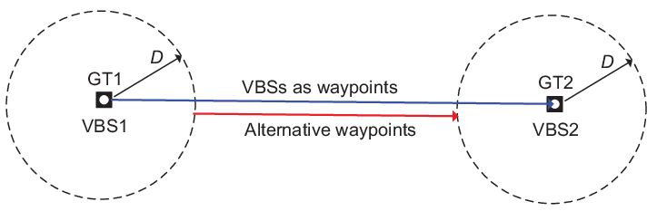
(3) Scheme 3 (proposed): Waypoints Based on VBS Placement and Convex Optimization. Traversing over all the $G$ VBSs, though providing a feasible waypoints design to $\mathrm{(P3)}$, may not always be desirable. This is illustrated by a toy example shown in Fig. 3, where there are two GTs, each covered by one VBS that is placed in essentially the same location as the GT. It is observed that traversing over both VBSs in fact leads to unnecessarily longer trajectory than the alternative design shown in Fig. 3. To overcome this limitation, in this subsection, we propose a more efficient waypoint design based on the placed VBSs and by applying convex optimization techniques.

Specifically, with VBS placement and TSP algorithm applied over the obtained $G$ VBSs, the GTs in $\mathcal{K}$ are essentially partitioned into $G$ ordered clusters $\mathcal{S}_{g}$, $g=1,\cdots,G$, where $\mathcal{S}_{g}\subset\mathcal{K}$ denotes the subset of GTs that are covered by the $g$th VBS while applying the VBS placement algorithm. For the $g$th ordered cluster with GTs $\mathcal{S}_{g}$, define the following set

In other words, $\mathcal{C}_{g}$ is the set of all possible UAV locations ensuring that all GTs in $\mathcal{S}_{g}$ are simultaneously in connection with the UAV. It is obvious that $\mathcal{C}_{g}$ is non-empty (since the VBS $g$ with location $\mathbf{v}_{g}$ belongs to this set) and a convex set (since it is an intersection of $|\mathcal{S}_{g}|$ convex sets). As a result, as long as the UAV sequentially visits all the $G$ convex regions $\mathcal{C}_{g}$, the constraints in (30) can be met by appropriate UAV speed optimization. In the following, the waypoints in each of the convex region $\mathcal{C}_{g}$ is optimized.

Without loss of generality, let $\mathbf{s}_{g},\mathbf{f}_{g}\in\mathcal{C}_{g}$ be the starting and ending points of the UAV trajectory intersecting with the region $\mathcal{C}_{g}$, respectively. Note that since $\mathcal{C}_{g}$ is a convex set, all points on the line segment between $\mathbf{s}_{g}$ and $\mathbf{f}_{g}$ are also in $\mathcal{C}_{g}$, i.e., they ensure that all the GTs in $\mathcal{S}_{g}$ are in connection with the UAV. Given the UAV’s maximum flying speed $V_{\max}$, the minimum time required for the UAV to travel within the region $\mathcal{C}_{g}$, i.e., from $\mathbf{s}_{g}$ to $\mathbf{f}_{g}$, is $\frac{\|\mathbf{f}_{g}-\mathbf{s}_{g}\|}{V_{\max}}$. On the other hand, to ensure the minimum connection time constraint (30), one viable approach is to ensure that the UAV remains in $\mathcal{C}_{g}$ for at least $T_{\min}$ seconds. Thus, the minimum time required for the UAV to travel within $\mathcal{C}_{g}$ is $\max\left\{\frac{\|\mathbf{f}_{g}-\mathbf{s}_{g}\|}{V_{\max}},T_{\min}\right\}$. Furthermore, the minimum time required for the UAV to travel between $\mathcal{C}_{g}$ and $\mathcal{C}_{g+1}$ is $\frac{\|\mathbf{s}_{g+1}-\mathbf{f}_{g}\|}{V_{\max}}$. As a result, the waypoints $\{\mathbf{s}_{g},\mathbf{f}_{g}\}_{g=1}^{G}$ could be designed by solving the following problem

Note that the cost function of $\mathrm{(P4)}$ is the total mission completion time with waypoints $\{\mathbf{s}_{g},\mathbf{f}_{g}\}$, which is a convex function with respect to $\{\mathbf{s}_{g},\mathbf{f}_{g}\}$. Furthermore, all the constraints in $\mathrm{(P4)}$ are convex. Thus, $\mathrm{(P4)}$ is a convex optimization problem, which can be efficiently solved by standard convex optimization techniques or existing software such as CVX [37].

Note that as compared to the previous scheme by directly taking the VBSs as waypoints, the new waypoints obtained in $\mathrm{(P4)}$ avoid the unnecessary traveling to the VBSs, and thus are expected to achieve better performance, as will be numerically verified in Section V.

For any given set of feasible waypoints $\mathcal{Q}_{\mathrm{wp}}$, the UAV path is determined by sequentially connecting the waypoints $\mathcal{Q}_{\mathrm{wp}}$ with line segments. As a result, problem $\mathrm{(P3)}$ reduces to finding the optimal instantaneous UAV speed over time along the path connecting these waypoints. To this end, we discretize the UAV path with the infinitesimal displacement $\delta_{d}$ (instead of over time) to get $J$ UAV sampled locations on the path, denoted by $\{\mathbf{q}_{j}\}_{j=1}^{J}$. As a result, the corresponding value of the indicator function in (32) can be obtained, which is denoted as $I_{kj}$, $k\in\mathcal{K}$, $j=1,\cdots,J$. That is, $I_{kj}=1$ represents that the UAV is in connection with GT $k$ when it is at location $j$. Denote by $\tau_{j}\geq 0$ the time for the UAV to travel from location $\mathbf{q}_{j}$ to $\mathbf{q}_{j+1}$, with the speed $V_{j}=\frac{\delta_{d}}{\tau_{j}}$. Note that since $\delta_{d}$ is set sufficiently small, $V_{j}$ well approximates the instantaneous UAV speed, and we must have $\frac{\delta_{d}}{\tau_{j}}\leq V_{\max}$. For any given set of feasible waypoints, $\mathrm{(P3)}$ reduces to optimizing the UAV speed $V_{j}$ or equivalently the time duration $\tau_{j}$, $j=1,\cdots,J$, which is formulated as

Note that $\mathrm{(P5)}$ is feasible if and only if $\forall k\in\mathcal{K}$, there exists at least one UAV location $j$ such that $I_{kj}=1$. This is guaranteed based on the three waypoint designs presented in Section IV-A. $\mathrm{(P5)}$ is a standard LP problem, which can be efficiently solved via e.g. [37].

By choosing the auxiliary distance parameter as $D=400$m, Fig. 4 compares the different UAV trajectories with the four considered waypoint designs for one specific realization of the GT locations with $K=50$. The corresponding total UAV traveling distances $d_{\mathrm{tr}}$ and the mission completion time $T$ are also shown in the figure. It is observed that for both benchmark schemes with strip-based waypoints and GTs as waypoints, the UAV needs to travel longer distances and hence require larger mission completion time, as compared to the proposed designs as shown in Fig. 4(c) and Fig. 4(d). This is expected since compared to the two benchmark schemes, the proposed designs jointly utilize the information of the GT locations and the coverage distance $D$ via VBS placement and convex optimization. Furthermore, by comparing Fig. 4(c) and Fig. 4(d), it is observed that by solving the convex optimization problem $\mathrm{(P4)}$ based on the obtained VBSs, the UAV can further reduce its required traveling distance and mission completion time by avoiding the unnecessary visit to all the VBSs.

For the proposed UAV trajectory shown in Fig. 4(d), Fig. 5 plots the actual file recovery probability $P_{k,\mathrm{succ}}$ and our derived lower bound $P_{k,\mathrm{lb}}$, where $P_{k,\mathrm{succ}}$ is obtained numerically via Monte Carlo simulations over $10^{4}$ random channel realizations. Note that for better visualization, only the results for 10 of the GTs are shown in the figure. It is observed that with the proposed UAV trajectory design, the constraints in (22) based on the lower bound of the file recovery probability are satisfied with strict equality for some of the GTs, as expected. Furthermore, it is found that with the optimized UAV trajectory, all GTs are able to successfully recover the file almost surely, i.e., with actual success probability almost equal to 1. This verifies the proposed lower bound and also shows the effectiveness of the proposed trajectory design.

Next, we study the effect of the auxiliary distance parameter $D$ on the system performance. Fig. 6 plots the total mission completion time versus $D$ for the four UAV trajectory design schemes, with the GT locations same as Fig. 4. It is observed that for all schemes, the mission completion time has the general trend of firstly decreasing and then increasing with $D$. This is expected since the value of $D$ affects the UAV trajectory design in two different ways. On one hand, increasing $D$ leads to lower successful packet reception probability $p_{D}$ in (14), which in turn requires that each GT to keep in connection with the UAV for a longer duration in order to ensure the same file recovery probability. From this perspective, the mission completion time tends to increase with $D$. On the other hand, as $D$ increases, there will be more GTs that are simultaneously in connection with the UAV. As a result, the UAV in general needs to travel shorter distances if larger $D$ is chosen. From this perspective, the mission completion time tends to decrease with the increasing of $D$. Thus, for any given GT locations, there exists an optimal threshold distance $D$ that balances the above two conflicting effects and achieves the minimum mission completion time. To our best effort, it is challenging to find the optimal value $D$ analytically. However, as illustrated in Fig. 6, one good choice for $D$ is such that the average received SNR when the GT and UAV are separated by horizontal distance $D$ is equal to the threshold SNR $\bar{\gamma}_{\mathrm{th}}$, in which case $D$ is given by $D^{*}$ in (9). For the setup under consideration, we have $D^{*}=430.3$m, which gives the near optimal choice based on Fig. 6.

Fig. 7 compares the average mission completion time versus the number of GTs $K$, where the average is taken over $100$ random realizations of the GT locations. For all schemes, the auxiliary distance parameter $D$ is set as $D^{*}=430.3$m. It is first observed that for small or moderate number of GTs, all the three trajectories with the waypoints designs given in Section IV-A significantly outperform the benchmark strip-based trajectory. This is expected since when the GTs are sparsely distributed, utilizing the location information of the GTs more wisely is beneficial for the UAV trajectory design. As $K$ increases or the GTs are more densely deployed, the trajectory design by simply taking the GTs as the waypoints performs worse than the other benchmark scheme with strip-based waypoints, since it becomes time wasteful for the UAV to visit all the GTs even when many of them are near to each other. For all the $K$ values considered, both proposed designs with the VBSs as waypoints or with the optimized waypoints significantly outperform the two benchmark schemes. For instance, for $K=80$, the mission completion time with the two proposed trajectory designs is reduced by around $50\%$ as compared to the benchmark scheme with GTs as waypoints, and by $30\%$ than the strip-based waypoints design.

Last, to illustrate the performance gain by exploiting the high UAV mobility, we consider another benchmark multicasting scheme with static transmitter, i.e., the horizontal projection of the transmitter (e.g., a static UAV) is fixed at the geometric center of the GTs. For $K=100$ GTs, Fig. 8 shows the number of successful GTs (i.e., those with successful file recovery probability no smaller than $\bar{P}$) for the benchmark scheme with a static transmitter as the transmission time increases. It is observed that although the number of successful GTs increases with the transmission time, or equivalently with the number of transmitted coded packets, the increasing rate is very slow. For example, even with the transmission time increased to $10^{4}$ s, only $23$ GTs are able to achieve the targeting file recovery probability. This is expected since with the transmitter fixed in location, the GTs that have a long distance with the transmitter suffer from high packet loss probabilities. On the other hand, with UAV-enabled multicasting with the proposed trajectory design, only about $210$s is needed to ensure that all the $100$ GTs satisfy the file recovery requirement, as can be seen from Fig. 7. This demonstrates the dramatic performance gain by exploiting the high mobility of UAVs for wireless multicasting.

References

- [1] A. Osseiran et al., “Scenarios for 5G mobile and wireless communications: the vision of the METIS project,” IEEE Commun. Mag., vol. 52, no. 5, pp. 26–35, May 2014.
- [2] “Project Loon”, Available online at https://x.company/loon/.
- [3] S. Chandrasekharan et al., “Designing and implementing future aerial communication networks,” IEEE Commun. Mag., vol. 54, no. 5, pp. 26–34, May 2016.
- [4] “The technology behind Aquila”, Available online at https://www.facebook.com/notes/mark-zuckerberg/the-technology-behind-aquila/10153916136506634/.
- [5] Y. Zeng, R. Zhang, and T. J. Lim, “Wireless communications with unmanned aerial vehicles: opportunities and challenges,” IEEE Commun. Mag., vol. 54, no. 5, pp. 36–42, May 2016.
- [6] A. Al-Hourani, S. Kandeepan, and S. Lardner, “Optimal LAP altitude for maximum coverage,” IEEE Wireless Commun. Lett., vol. 3, no. 6, pp. 569–572, Dec. 2014.
- [7] V. Sharma, M. Bennis, and R. Kumar, “UAV-assisted heterogeneous networks for capacity enhancement,” IEEE Commun. Letters, vol. 20, no. 6, pp. 1207–1210, Apr. 2016.
- [8] R. Yaliniz, A. El-Keyi, and H. Yanikomeroglu, “Efficient 3-D placement of an aerial base station in next generation cellular networks,” in Proc. IEEE Int. Conf. Commun. (ICC), Kuala Lumpur, Malaysia, May 2016.
- [9] M. Mozaffari, W. Saad, M. Bennis, and M. Debbah, “Efficient deployment of multiple unmanned aerial vehicles for optimal wireless coverage,” IEEE Commun. Letters, vol. 20, no. 8, pp. 1647–1650, Aug. 2016.
- [10] E. Kalantari, H. Yanikomeroglu, and A. Yongacoglu, “On the number and 3D placement of drone base stations in wireless cellular networks,” in Proc. Vehicular Techn. Conf. (VTC-Fall), Sep. 18-21, 2016.
- [11] J. Lyu, Y. Zeng, R. Zhang, and T. J. Lim, “Placement optimization of UAV-mounted mobile base stations,” IEEE Commun. Letters, vol. 21, no. 3, pp. 604–607, Mar. 2017.
- [12] M. M. Azari, F. Rosas, K. C. Chen, and S. Pollin, “Optimal UAV positioning for terrestrial-aerial communication in presence of fading,” in Proc. IEEE Global Commun. Conf. (GLOBECOM), Dec. 4-8, 2016.
- [13] J. Chen and D. Gesbert, “Optimal positioning of flying relays for wireless networks: A LOS map approach,” in Proc. IEEE Int. Conf. Commun. (ICC), May 21-25, 2017.
- [14] Y. Zeng, R. Zhang, and T. J. Lim, “Throughput maximization for UAV-enabled mobile relaying systems,” IEEE Trans. Commun., vol. 64, no. 12, pp. 4983–4996, Dec. 2016.
- [15] C. Zhan, Y. Zeng, and R. Zhang, “Energy-efficient data collection in UAV enabled wireless sensor network,” submitted to IEEE Wireless Commun. Letters, available online at https://arxiv.org/abs/1708.00221.
- [16] M. Mozaffari, W. Saad, M. Bennis, and M. Debbah, “Mobile internet of things: Can UAVs provide an energy-efficient mobile architecture,” in Proc. IEEE Global Commun. Conf. (GLOBECOM), Dec. 2016.
- [17] J. Lyu, Y. Zeng, and R. Zhang, “Cyclical multiple access in UAV-aided communications: a throughput-delay tradeoff,” IEEE Wireless Commun. Letters, vol. 5, no. 6, pp. 600–603, Dec. 2016.
- [18] T. Schouwenaars, B. D. Moor, E. Feron, and J. How, “Mixed integer programming for multi-vehicle path planning,” in Proc. European Control Conf., pp. 2603–2608, 2001.
- [19] A. Richards and J. P. How, “Aircraft trajectory planning with collision avoidance using mixed integer linear programming,” in Proc. American Control Conf., pp. 1936–1941, May 8-10, 2002.
- [20] I. K. Nikolos, N. C. Tsourveloudis, and K. P. Valavanis, “Evolutionary algorithm based offline/online path planner for UAV navigation,” IEEE Trans. Syst. Man Cybern., Part B, Cybern., vol. 33, no. 6, pp. 898–912, Dec. 2003.
- [21] C. Zheng, L. Li, F. Xu, F. Sun, and M. Ding, “Evolutionary route planner for unmanned air vehicles,” IEEE Trans. Robotics, vol. 21, no. 4, pp. 609–620, Aug. 2005.
- [22] F. Jiang and A. L. Swindlehurst, “Optimization of UAV heading for the ground-to-air uplink,” IEEE J. Sel. Areas Commun., vol. 30, no. 5, pp. 993–1005, Jun. 2012.
- [23] Y. Zeng and R. Zhang, “Energy-efficient UAV communication with trajectory optimization,” IEEE Trans. Wireless Commun., vol. 16, no. 6, pp. 3747–3760, Jun. 2017.
- [24] Q. Wu, Y. Zeng, and R. Zhang, “Joint trajectory and communication design for multi-UAV enabled wireless networks,” submitted to IEEE Trans. Wireless Commun., available online at https://arxiv.org/abs/1705.02723.
- [25] Y. Zeng, X. Xu, and R. Zhang, “Exploiting mobility for UAV-enabled multicasting,” submitted to IEEE Wireless Commun. and Netw. Conf. (WCNC), Barcelona, Spain, April 15-18, 2018.
- [26] A. Merwaday and I. Guvenc, “UAV assisted heterogeneous networks for public safety communications,” in Proc. IEEE Wireless Commun. Netw. Conf. (WCNC), pp. 329–334, Mar. 9-12, 2015.
- [27] X. Wang, A. Chowdhery, and M. Chiang, “SkyEyes: adaptive video streaming from UAVs,” in Proc. 3rd Workshop on Hot Topics in Wireless, Oct. 3-7, 2016, pp. 2–6.
- [28] B. V. Bergh, A. Chiumento, and S. Pollin, “Ultra-reliable IEEE 802.11 for UAV video streaming: from network to application,” Advances in Ubiquitous Networking 2, pp. 637–647, Nov. 2016.
- [29] H. Menour, et al., “UAV-enabled intelligent transportation systems for the smart city: applications and challenges,” IEEE Commun. Mag., vol. 55, no. 3, pp. 22–28, Mar. 2017.
- [30] T. Ho, et al., “A random linear network coding approach to multicast,” IEEE Trans. Inf. Theory, vol. 52, no. 10, pp. 4413–4430, Oct. 2006.
- [31] G. Laporte, “The traveling salesman problem: an overview of exact and approximate algorithms,” EUR. J. Oper. Res., vol. 59, no. 2, pp. 231–247, Jun. 1992.
- [32] E. L. Lawler, J. K. Lenstra, A. H. G. R. Kan, and D. B. Shmoys, The Traveling Salesman Problem: A Guided Tour of Combinatorial Optimization, 1st ed. Wiley, 1985.
- [33] “Travelling Salesman Problem”, Availabe online at https://www.mathworks.com/help/optim/ug/travelling-salesman-problem.html.
- [34] Y. H. Wang, “On the number of successes in independent trials,” Statistica Sinica, vol. 3, no. 2, pp. 295–312, Jul. 1993.
- [35] A. Dumitrscu and J. Mitchell, “Approximation algorithms for TSP with neighborhoods in the plane,” J. Algorithms, vol. 48, no. 1, pp. 135–159, 2003.
- [36] B. Yuan, M. Orlowska, and S. Sadiq, “On the optimal robot routing problem in wireless sensor networks,” IEEE Trans. Knowledge and Data Eng., vol. 19, no. 9, pp. 1252–1261, Sep. 2007.
- [37] M. Grant and S. Boyd, CVX: Matlab software for disciplined convex programming, version 2.1, http://cvxr.com/cvx.
- [38] C. Rego, D. Gamboa, F. Glover, and C. Osterman, “Traveling salesman problem heuristics: leading methods, implementations and latest advances,” European Journal of Operational Research, vol. 211, no. 3, pp. 427–441, 2011.
- [39] S. Boyd and L. Vandenberghe, Convex Optimization. Cambridge, U.K.: Cambridge Univ. Press, 2004.