Device-Aware Routing and Scheduling in Multi-Hop Device-to-Device Networks

We consider a multi-hop D2D network with mobile devices, where devices are connected to each other via D2D connections. In this setup, packets from a source device traverse potentially multiple devices before arriving to the destination device. Devices in this setup are capable of performing various tasks including routing, scheduling, and rate control. However, depending on device capabilities and configurations, the transmission rates vary. Our system model, and algorithm design capture this heterogeneity. In this section, we provide an overview of this setup and highlight some of its key characteristics.¹¹ 1 We note that this section introduces our setup and assumptions needed for the theoretical development of our device-aware framework. We will revise some of these assumptions in Section IV when we discuss implementation details of our algorithm in a testbed.

Setup: We consider a multi-hop D2D network, which consists of $N$ devices and $L$ edges, where $\mathcal{N}$ and $\mathcal{L}$ are the set of nodes and edges, respectively. We consider in our formulation and analysis that time is slotted, and $t$ refers to the beginning of slot $t$.

Sources and Flows: Let $\mathcal{S}$ be the set of unicast flows between source and destination device pairs. Each flow $s\in\mathcal{S}$ generates $A_{s}(t)$ packets at the application layer at time $t$.

The packet arrivals are i.i.d. over the slots and the first and second moments of the arrival distribution is finite; i.e., $\lambda_{s}=E[A_{s}(t)]$, and $E[A_{s}(t)^{2}]$. Packets are stored at the source device in an initial buffer in the application layer. Each flow $s$ is associated with rate $x_{s}$ and a utility function $g_{s}(x_{s})$, which we assume to be a strictly concave function of $x_{s}$ for our analysis purposes. Packets from the initial buffer are passed to the main buffer with rate $x_{s}(t)$ at time $t$ and depending on the utility function $g_{s}(x_{s}(t))$.

At time $t$, $f_{i,j}^{s}(t)$ packets from flow $s$ are passed from node $i$ to node $j$. The number of packets, i.e., $f_{i,j}^{s}(t)$, are determined by device-aware framework by taking into account device capabilities.

Now, we formulate our device-aware framework. Our objective is to determine $\boldsymbol{x},\boldsymbol{f}$, where $\boldsymbol{x}=\{x_{s}\}_{s\in\mathcal{S}}$, and $\boldsymbol{f}=\{f_{i,j}^{s}\}_{s\in\mathcal{S},(i,j)\in\mathcal{L}}$, by maximizing the total utility function; $\sum_{s\in\mathcal{S}}g_{s}(x_{s})$ subject to the constraints²² 2 Note that, in this section, we optimize the average values of the parameters defined in Section II-A. Thus, by abuse of notation, we use a variable, e.g., $\phi$ as the average value of $\phi(t)$ if both $\phi$ and $\phi(t)$ refers to the same parameter.

The first constraint in (1) is the flow conservation at device $i$ and for flow $s$, where $\sum_{j\in\mathcal{N}}f_{j,i}^{s}+x_{s}1_{[i=o(s)]}$ is the arrival rate of flow $s$ to node $i$, while $\sum_{j\in\mathcal{N}}f_{i,j}^{s}$ is the departure rate.

The second constraint captures device capabilities. The arrival rate to device $j$, i.e., $\sum_{s\in\mathcal{S}}\sum_{i\in\mathcal{N}}f_{i,j}^{s}$ should be supported by the device, where $R_{P}^{j}$ is the maximum rate that device $j$ can support (receive and transmit) with its computing power, while $R_{E}^{j}$ and $R_{W}^{j}$ are the rates that device $j$ can support by with its energy and incentives, respectively.

The last constraint in (1) is the feasibility constraint, where $\boldsymbol{\Gamma}$ is the set of all feasible rates that can be in the network. Thus, $\boldsymbol{f}$ should be an element of $\boldsymbol{\Gamma}$.

Although the solution of (1) provides a device-aware routing and scheduling, the solution is not practical, because it requires an active involvement of all devices in D2D network even if a device does not prefer any involvement. For example, even if a node $j$ has very small $\min\{R_{P}^{j},R_{E}^{j},R_{W}^{j}\}$, it needs to periodically update the other devices in the network about its status (whether it can relay packets or not), which is not practical and introduces overhead. Thus, we modify the problem in (1) so that the solution can be more practical.

Our first step is to explicitly involve link rates in the formulation. Assume that $R_{i,j}$ is the transmission rate between nodes $i,j$ and $\tau_{i,j}$ is the percentage of time that the link $i-j$ is used. Then, we can express $f_{i,j}^{s}=R_{i,j}\tau_{i,j}^{s}$, $\forall i\in\mathcal{N},j\in\mathcal{N},s\in\mathcal{S}$. This translates the constraints in (1) to $\sum_{j\in\mathcal{N}}R_{i,j}\tau_{i,j}^{s}-\sum_{j\in\mathcal{N}}R_{j,i}\tau_{j,i}^{s}=x_{s}1_{[i=o(s)]},\mbox{ }\forall s\in\mathcal{S},i\in\mathcal{N}$, $\sum_{s\in\mathcal{S}}\sum_{i\in\mathcal{N}}R_{i,j}\tau_{i,j}^{s}\leq\min\{R_{P}^{j},R_{E}^{j},R_{W}^{j}\},\forall j\in\mathcal{N}$ , and $\boldsymbol{\tau}\in\boldsymbol{\Gamma}_{\tau}$, where $\boldsymbol{\tau}=\{\tau_{i,j}^{s}\}_{s\in\mathcal{S},(i,j)\in\mathcal{L}}$, and $\boldsymbol{\Gamma}_{\tau}$ is the set of all feasible link schedules, so $\boldsymbol{\tau}\in\boldsymbol{\Gamma}_{\tau}$ should hold.

The next step is to create a new variable $\gamma_{i,j}^{s}$ as $\gamma_{i,j}^{s}$ $=$ $\tau_{i,j}^{s}$ $\frac{R_{i,j}}{\min\{R_{E}^{j},R_{W}^{j},R_{P}^{j}\}}$ assuming that $\min\{R_{P}^{j},R_{E}^{j},R_{W}^{j}\}$ is positive, at least slightly larger than 0. Then, the constraints become

where $\boldsymbol{\gamma}=\{\gamma_{i,j}^{s}\}_{s\in\mathcal{S},(i,j)\in\mathcal{L}}$, and $\boldsymbol{\Gamma}_{\gamma}$ is the set of feasible $\boldsymbol{\gamma}$’s. Next, we provide a solution to the problem of maximizing the total utility; $\sum_{s\in\mathcal{S}}g_{s}(x_{s})$ subject to the constraints in (2).

Lagrangian relaxation of the first constraint of (2) gives the following Lagrange function:

where $u_{i}^{s}$ is the Lagrange multiplier. The Lagrange function is expressed as

This Lagrange function is decomposed into two sub-problems: (i) rate control, and (ii) routing and scheduling. If we solve the Lagrangian function with respect to $x_{s}$, we have an optimization problem: $\max_{\boldsymbol{x}}\sum_{s\in\mathcal{S}}[g_{s}(x_{s})-u_{o(s)}^{s}x_{s}]$, which is the rate control part. On the other hand, the routing and scheduling part solves the following optimization problem

Note that the solution of (5) is easier as compared to the solution of (1), because it reduces to selecting the link $i-j$, which maximizes $\min\{R_{E}^{j},R_{W}^{j},R_{P}^{j}\}(u_{i}^{s}-u_{j}^{s})$ among all feasible schedules of links. Based on this idea, we will develop our device-aware stochastic routing and scheduling algorithm in the next section.

Wi-Fi Direct: Our approach to create multi-hop topology using Android-based devices is to employ Wi-Fi Direct connections [4]. However, existing Wi-Fi Direct implementation in Android-based devices only supports a star topology as shown in Fig. 6(a), but not any other multi-hop topology.

Our Approach: We use the star topology of Wi-Fi Direct shown in Fig. 6(a) as our basic constructing unit for creating multi-hop topologies. In particular, multiple groups are constructed using the star topology (i.e., each group is a star topology), and these groups are connected to each other. Connecting multiple groups (star topologies) is quite challenging, because the star topology of Wi-Fi Direct is constructed in a way that one device (center of the topology) is a group owner (GO), and the other devices are clients. In this setup, a device cannot act as both a group owner and a client simultaneously, which makes connecting multiple groups to each other prohibitively difficult.

In our testbed, we use legacy Wi-Fi interface to connect multiple groups. Let us consider Fig. 6(b), where there are two groups; Group I: $D_{1}$, $D_{2}$ and Group II: $D_{3}$, $D_{4}$. In this example, $D_{1}$ and $D_{3}$ are group owners, and $D_{2}$ and $D_{4}$ are clients of Group I and Group II, respectively. Let us assume that our goal is to connect $D_{2}$ and $D_{3}$. In existing Wi-Fi Direct, $D_{2}$ cannot connect to $D_{3}$ as $D_{2}$ can only connect to its group owner (which is $D_{1}$) via Wi-Fi Direct interface. On the other hand, $D_{3}$ cannot connect to $D_{2}$ as a client, because $D_{3}$ is already a group owner of Group II, so it cannot be a client of $D_{2}$. Therefore, our approach is to use legacy Wi-Fi interface of $D_{2}$ to connect to $D_{3}$. This connection is possible as $D_{2}$ will see $D_{3}$ as an access point of the legacy Wi-Fi connection. Thus, $D_{2}$ can connect to $D_{3}$, which provides a line topology consisting of 4 nodes, which was not possible by using only existing Wi-Fi Direct setup.

Similarly, we can create other multi-hop topologies. For example, we can create a diamond topology as shown in Fig. 6(c), where $D_{1}$ and $D_{4}$ are group owners, and $D_{2}$ and $D_{3}$ are clients in Wi-Fi Direct groups. $D_{2}$ and $D_{3}$ are connected to $D_{1}$ via Wi-Fi Direct interface, and connect to $D_{4}$ using their legacy Wi-Fi interfaces.

Our approach of using legacy Wi-Fi interfaces simultaneously with Wi-Fi Direct interfaces is challenging, because both legacy Wi-Fi interface and Wi-Fi Direct interfaces are actually using the same means of communication interface in the MAC layer, which is 802.11. Thus, if we naively open both legacy Wi-Fi and Wi-Fi Direct interfaces, only one of them will operate due to IP addressing conflicts. For example, $D_{2}$ would transmit data to $D_{1}$ even if it means to transmit to $D_{3}$ in Fig. 6(b). We provide a solution to this problem in a simple way (i.e., without rooting mobile devices). In particular, we use a class called ConnectivityManager in Android API, which provides instances (objects of the class) of all active network interfaces on each device. Thus, we access the instance of legacy Wi-Fi interface, and bind it with transmission sockets TCP or UDP. This approach eliminates addressing issues and conflicts between legacy Wi-Fi and Wi-Fi Direct interfaces.

In this section, we present how DARS is implemented over our multi-hop testbed described in Section IV-A.

Devices: We implemented a testbed of the different topologies including line topology, diamond topology using real mobile devices, specifically Android 5.1.1 based Nexus 5 smartphones and Nexus 7 tablets.

Integration to the Protocol Stack: We implemented DARS as a slim layer between transport and application layers as demonstrated in Fig. 7. In other words, we implemented DARS on top of TCP. This kind of implementation has benefits as (i) mobile devices do not require rooting, and (ii) our DARS codes could be easily transferred to mobile devices using other operating systems such as iOS.

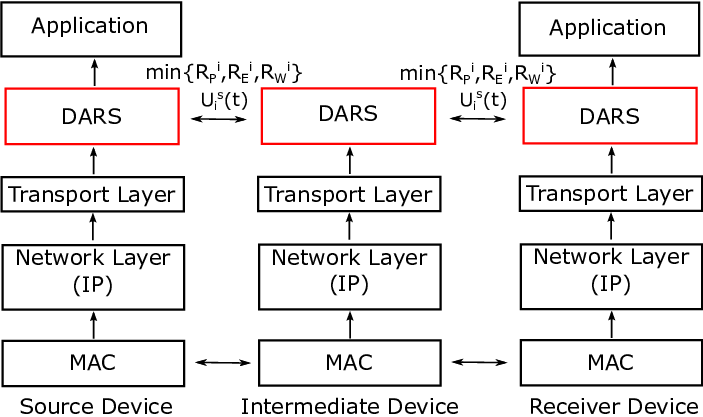
Virtual Slots: As mentioned in Section II, DARS uses slots to make transmission decisions. By following the theory, in our implementation, we divided the time into virtual slots. Each decision is made at the start of the slot. We set slot durations to 50msec.

Multiple Threads: Three sets of threads operate at each device simultaneously to perform the tasks of rate control, routing and scheduling, and actual data transmission.

The first set of threads are implemented for the rate control, so we call them rate control threads. In particular, the rate control thread at the source device $o(s)$ reads data bytes from a file, packetizes them and inserts them into the transmission queue $U_{o(s)}^{s}$. The rate of reading packets from the file is determined according to the rate control algorithm in (6). Note that if a device is the source of two flows, a rate control thread is created for each flow.

The second set of threads determine how many packets should be transmitted from $U_{i}^{s}$ to other devices. Thus, these threads are called routing and scheduling threads. This part implements (7). For example, in the diamond topology in Fig. 6(d), at each slot, $D_{1}$ determines whether it should transmit packets to $D_{2}$, or $D_{3}$, or none of them.

The final set of threads make actual packet transmissions possible, so we call them transmission threads. A transmission thread is constructed for each neighboring node. For example, in the diamond topology Fig. 6(c), $D_{1}$ constructs two transmission threads for $D_{2}$ and $D_{3}$. Packets, whose number is determined by the routing and scheduling thread, are received by this thread and inserted into queues that we call socket queues. The transmission threads will dequeue packets from the socket queues and pass them to TCP sockets. Another task of transmission threads is to receive queue size information from neighboring nodes.

Information Exchange: Our implementation is lightweight in the sense that it limits control information exchange among mobile devices. The control information that is transmitted by node $i$ is $U_{i}^{s}(t)$ and $\min\{R_{P}^{i},R_{E}^{i},R_{W}^{i}\}$, and this information is transmitted to only $i$’s neighbors. These control packets are transmitted periodically at every 50msec.

Calculating $\min\{R_{P}^{i},R_{E}^{i},R_{W}^{i}\}$: Each node $i$, based on its computing power, energy level, and incentives (willingness), calculates its rate. For example, if node $i$ has limited energy, then it limits $R_{E}^{i}$ to 1Mbps even if it can support up to 20Mbps. Thus, in our implementation, every device calculates its own rate, and exchange this information with its neighbors.

Test Environment: We conducted our experiments in a lab environment where several other Wi-Fi networks were operating in the background. We located all the devices at varying distances, and we have evaluated device-centric routing and scheduling. Next, we present our evaluation results.

Now, we focus on evaluating the performance of DARS. Fig. 8(a) shows data rate versus time graph for three-node and four-node line topologies shown in Fig. 6(b), where a a flow is transmitted from $D_{1}$ to $D_{4}$. The receive & forward algorithm is the baseline in this scenario, where the intermediate nodes just receive packets and forward. As seen, the performance of DARS is close to receive & forward. Note that since there is no routing and scheduling diversity in the line topology, the receive & forward provides the best performance. The results prove that DARS does not introduce too much overhead into the system.

Fig. 8(b) shows the transmission rate for the diamond topology shown in Fig. 6(c), where a flow is transmitted from $D_{1}$ to $D_{4}$. In this setup, $D_{1}$, $D_{2}$, and $D_{4}$ are Nexus 5 smartphones, and $D_{3}$ is a Nexus 7 tablet. The computing power of Nexus 5 smartphones is better than Nexus 7 tablet. In particular, Nexus 5 supports two times faster rate as compared to Nexus 7. Thus, DARS should prefer $D_{1}-D_{2}-D_{4}$ route instead of $D_{1}-D_{3}-D_{4}$ when $D_{1}$ is the source and $D_{4}$ is the receiver. The simulation results support this as further explained next.

The best case scenario in Fig. 8(b) is the case that $D_{1}-D_{2}-D_{4}$ route is selected a priori. As seen, DARS performs very close to the best case scenario, which shows the efficiency of our algorithm. Backpressure is the implementation of the scheme proposed in [6]. As seen, DARS improves over backpressure (up to %15), because it takes into account device specific properties, while backpressure does not. Equal Split is another baseline, which allows transmitting data over both paths in the diamond topology. As long as TCP supports transmissions, packets are simultaneously transmitted over both links. As seen, DARS significantly improves as compared to this baseline. Finally, the worst case scenario is the case that $D_{1}-D_{3}-D_{4}$ route is selected a priori, which is included in the results for completeness.

References

- [1] “Cisco visual networking index: Global mobile data traffic forecast update,” 2014-2019.
- [2] “Ericsson mobility report,” February 2015.
- [3] A. Asadi, Q. Wang, and V. Mancuso, “A survey on device-to-device communication in cellular networks,” April 2014, technical report - arxiv:1310.0720v6[cs.GT].
- [4] “Wi-fi direct,” http://www.wi-fi.org/discover-and-learn/wi-fi-direct.
- [5] L. Tassiulas and A. Ephremides, “Stability properties of constrained queueing systems and scheduling policies for maximum throughput in mul- tihop radio networks,” IEEE Trans. on Automatic Control, vol. 37, no. 12, December 1992.
- [6] M. J. Neely, E. Modiano, and C. Li, “Fairness and optimal stochastic control for heterogeneous networks,” IEEE Trans. on Networking, vol. 16, no. 2, April 2008.
- [7] M. J. Neely, Stochastic network optimization with application to communication and queueing systems. Morgan & Claypool, 2010.
- [8] “A multilayer application for multi-hop messaging on android devices.” [Online]. Available: http://anrg.usc.edu/ee5792012/Group02/index.html
- [9] C. Casetti, C.-F. Chiasserini, L. C. Pelle, C. D. Valle, Y. Duan, and P. Giaccone, “Content-centric routing in wi-fi direct multi-group networks.” [Online]. Available: http://arxiv.org/abs/1412.0880
- [10] Y. Xing and H. Seferoglu, “Dars: Device-aware routing and scheduling in device-to-device networks - technical report.” [Online]. Available: http://nrl.ece.uic.edu/
- [11] S. Ioannidis, A. Chaintreau, and L. Massoulie, “Optimal and scalable distribution of content updates over a mobile social network,” in Proc. IEEE INFOCOM, Rio de Janeiro, Brazil, April 2009.
- [12] B. Han, P. Hui, V. A. Kumar, M. V. Marathe, G. Pei, and A. Srinivasan, “Cellular traffic offloading through opportunistic communications: a case study,” in Proc. of ACM Workshop on Challenged Networks (CHANTS), Chicago, IL, September 2010.
- [13] J. Whitbeck, M. Amorim, Y. Lopez, J. Leguay, and V. Conan, “Relieving the wireless infrastructure: When opportunistic networks meet guaranteed delays,” in Proc. of IEEE WoWMoM, Lucca, Italy, June 2011.
- [14] P. Hui, J. Crowcroft, and E. Yoneki, “Bubble rap: social-based forwarding in delay tolerant networks,” in Proc. of ACM MobiHoc, Hong Kong, May 2008.
- [15] C. Boldrini, M. Conti, and A. Passarella, “Exploiting users’ social relations to forward data in opportunistic networks: The hibop solution,” in Proc. of Pervasive and Mobile Computing, October 2008.
- [16] M. Ramadan, L. E. Zein, and Z. Dawy, “Implementation and evaluation of cooperative video streaming for mobile devices,” in Proc. of IEEE PIMRC, Cannes, France, September 2008.
- [17] S. Li and S. Chan, “Bopper: wireless video broadcasting with peer-to-peer error recovery,” in Proc. of IEEE ICME, Beijing, China, July 2007.
- [18] M. Chiang, S. T. Low, A. R. Calderbank, and J. C. Doyle, “Layering as optimization decomposition: a mathematical theory of network architectures,” Proceedings of the IEEE, vol. 95, no. 1, January 2007.
- [19] X. Lin, N. B. Schroff, and R. Srikant, “A tutorial on cross-layer optimization in wireless networks,” IEEE JSAC, vol. 24, no. 8, August 2006.
- [20] L. Tassiulas and A. Ephremides, “Dynamic server allocation to parallel queues with randomly varying connectivity,” IEEE Trans. on Information Theory, vol. 39, no. 2, March 1993.